Well, I was on the road for 1.5 days (work party for the Community Village at the Oregon Country Fair). As I was driving home, there was a magnitude M 5.6 earthquake in coastal northern California.
https://earthquake.usgs.gov/earthquakes/eventpage/nc73201181/executive
I didn’t realize this until I was almost home (finally hit the sack around 4 am).
This earthquake follows a sequence of quakes further to the northwest, however their timing is merely a coincidence. Let me repeat this. The M 5.6 earthquake is not related to the sequence of earthquakes along the Blanco fracture zone.
Contrary to what people have posted on social media, there was but a single earthquake. This earthquake happened beneath the area of Petrolia, nearby the 1991 Honeydew Earthquake. More about the Honeydew Earthquake can be found here.
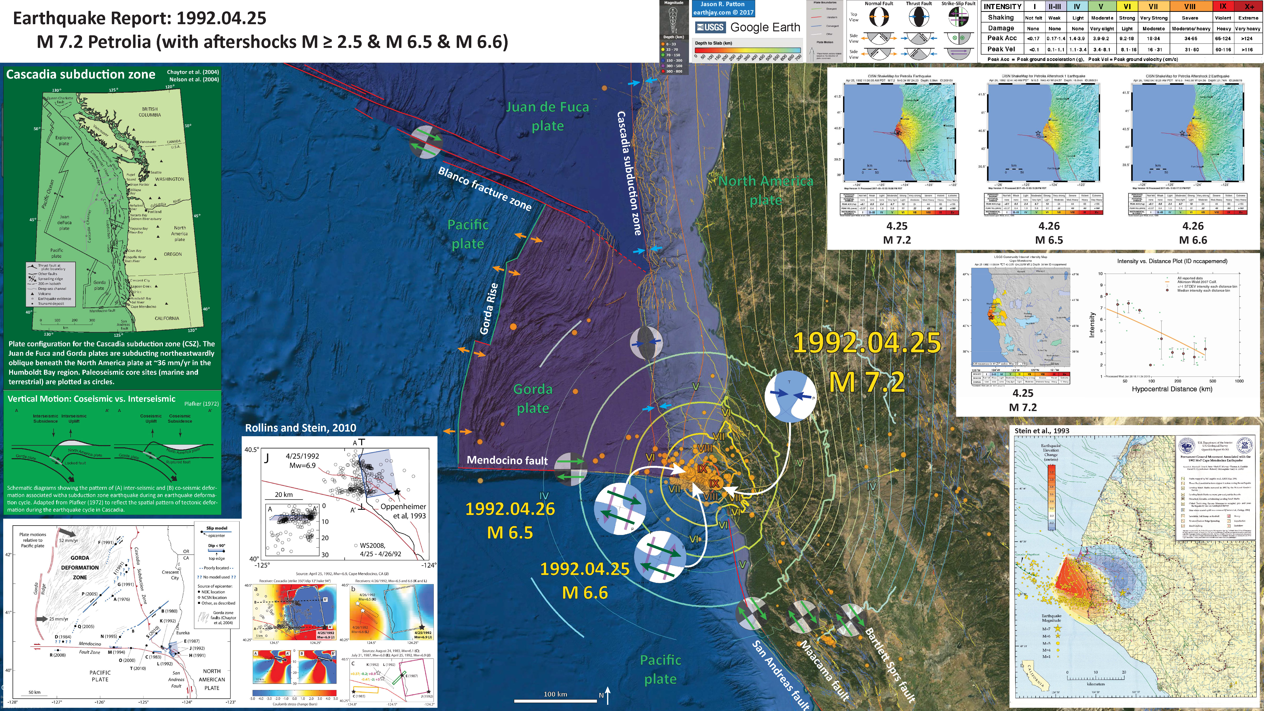
This region also had a good sized shaker in 1992, the Cape Mendocino Earthquake, which led to the development of the National Tsunami Hazard Mitigation Program. More about the Cape Mendocino Earthquake can be found on the 25th anniversary page here and in my earthquake report here.
The regional tectonics in coastal northern California are dominated by the Pacific-North America plate boundary. North of Cape Mendocino, this plate boundary is convergent and forms the Cascadia subduction zone (CSZ). To the south of Cape Mendocino, the plate boundary is the right-lateral (dextral) San Andreas fault (SAF). Where these 2 fault systems meet, there is another plate boundary system, the right-lateral strike-slip Mendocino fault (don’t write Mendocino fracture zone on your maps!). Where these 3 systems meet is called the Mendocino triple junction (MTJ).
The MTJ is a complicated region as these plate boundaries overlap in ways that we still do not fully understand. Geologic mapping in the mid- to late-20th century provides some basic understanding of the long term history. However, recent discoveries have proven that this early work needs to be revisited as there are many unanswered questions (and some of this early work has been demonstrated to be incorrect). Long live science!
Last night’s M 5.6 temblor happened where one strand of the MF trends onshore (another strand bends towards the south). But, it also is where the SAF trends onshore. At this point, I am associating this earthquake with the MF (so, a right-lateral strike-slip earthquake). The mechanism suggest that this is not a SAF related earthquake. However, it is oriented in a way that it could be in the Gorda plate (making it a left-lateral strike-slip earthquake). However, this quake is at the southern edge of the Gorda plate (sedge), so it is unlikely this is a Gorda plate event.
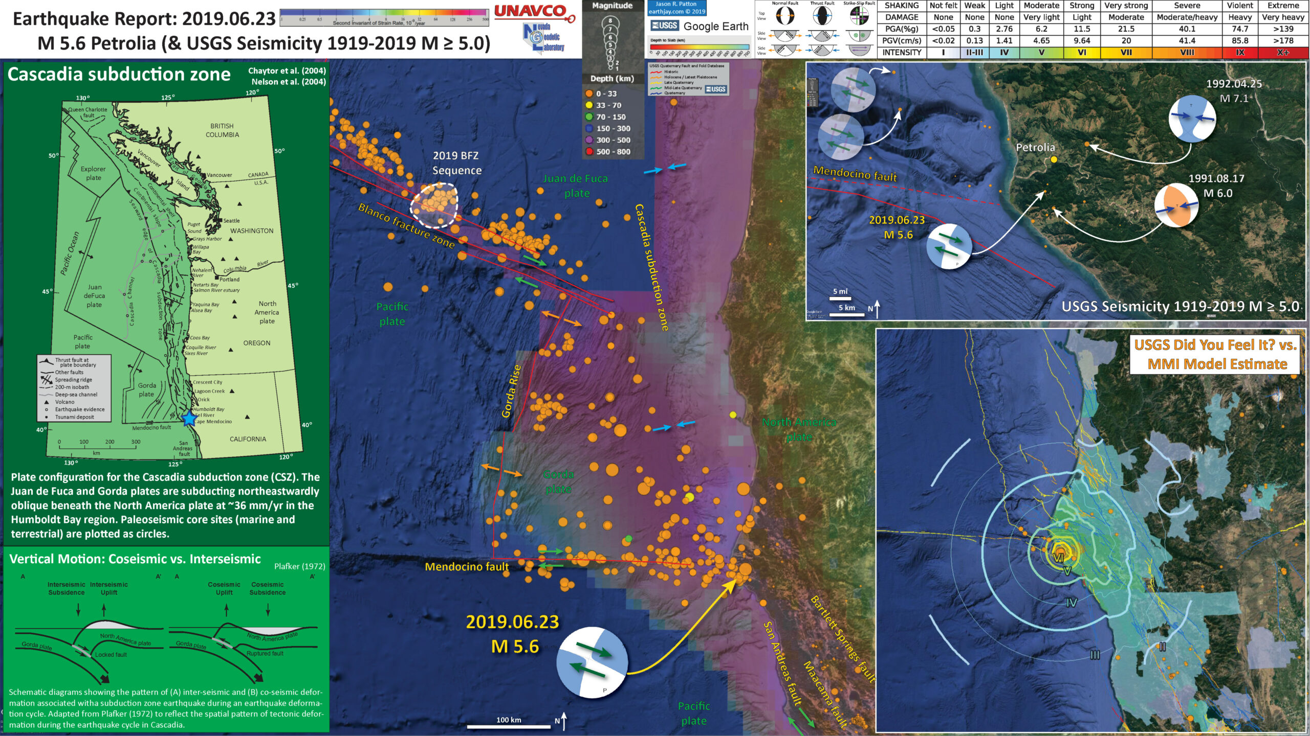
Below is my interpretive poster for this earthquake
I plot the seismicity from the past month, with color representing depth and diameter representing magnitude (see legend). I include earthquake epicenters from 1918-2018 with magnitudes M ≥ 5.0 in one version.
I plot the USGS fault plane solutions (moment tensors in blue and focal mechanisms in orange), possibly in addition to some relevant historic earthquakes.
- I placed a moment tensor / focal mechanism legend on the poster. There is more material from the USGS web sites about moment tensors and focal mechanisms (the beach ball symbols). Both moment tensors and focal mechanisms are solutions to seismologic data that reveal two possible interpretations for fault orientation and sense of motion. One must use other information, like the regional tectonics, to interpret which of the two possibilities is more likely.
- I also include the shaking intensity contours on the map. These use the Modified Mercalli Intensity Scale (MMI; see the legend on the map). This is based upon a computer model estimate of ground motions, different from the “Did You Feel It?” estimate of ground motions that is actually based on real observations. The MMI is a qualitative measure of shaking intensity. More on the MMI scale can be found here and here. This is based upon a computer model estimate of ground motions, different from the “Did You Feel It?” estimate of ground motions that is actually based on real observations.
- I include the slab 2.0 contours plotted (Hayes, 2018), which are contours that represent the depth to the subduction zone fault. These are mostly based upon seismicity. The depths of the earthquakes have considerable error and do not all occur along the subduction zone faults, so these slab contours are simply the best estimate for the location of the fault.
- In the map below, I include a transparent overlay of the magnetic anomaly data from EMAG2 (Meyer et al., 2017). As oceanic crust is formed, it inherits the magnetic field at the time. At different points through time, the magnetic polarity (north vs. south) flips, the North Pole becomes the South Pole. These changes in polarity can be seen when measuring the magnetic field above oceanic plates. This is one of the fundamental evidences for plate spreading at oceanic spreading ridges (like the Gorda rise).
- Regions with magnetic fields aligned like today’s magnetic polarity are colored red in the EMAG2 data, while reversed polarity regions are colored blue. Regions of intermediate magnetic field are colored light purple.
- We can see the roughly ~north-south trends of these red and blue stripes in the Pacific plate. These lines are parallel to the ocean spreading ridges from where they were formed. The stripes disappear at the subduction zone because the oceanic crust with these anomalies is diving deep beneath the North America plate, so the magnetic anomalies from the overlying Sunda plate mask the evidence for the Juan de Fuca and Gorda plates.
Magnetic Anomalies
- In a map below, I include a transparent overlay of the Global Strain Rate Map (Kreemer et al., 2014).
- The mission of the Global Strain Rate Map (GSRM) project is to determine a globally self-consistent strain rate and velocity field model, consistent with geodetic and geologic field observations. The overall mission also includes:
- contributions of global, regional, and local models by individual researchers
- archive existing data sets of geologic, geodetic, and seismic information that can contribute toward a greater understanding of strain phenomena
- archive existing methods for modeling strain rates and strain transients
- The completed global strain rate map will provide a large amount of information that is vital for our understanding of continental dynamics and for the quantification of seismic hazards.
- The version used in the poster(s) below is an update to the original 2004 map (Kreemer et al., 2000, 2003; Holt et al., 2005).
Global Strain
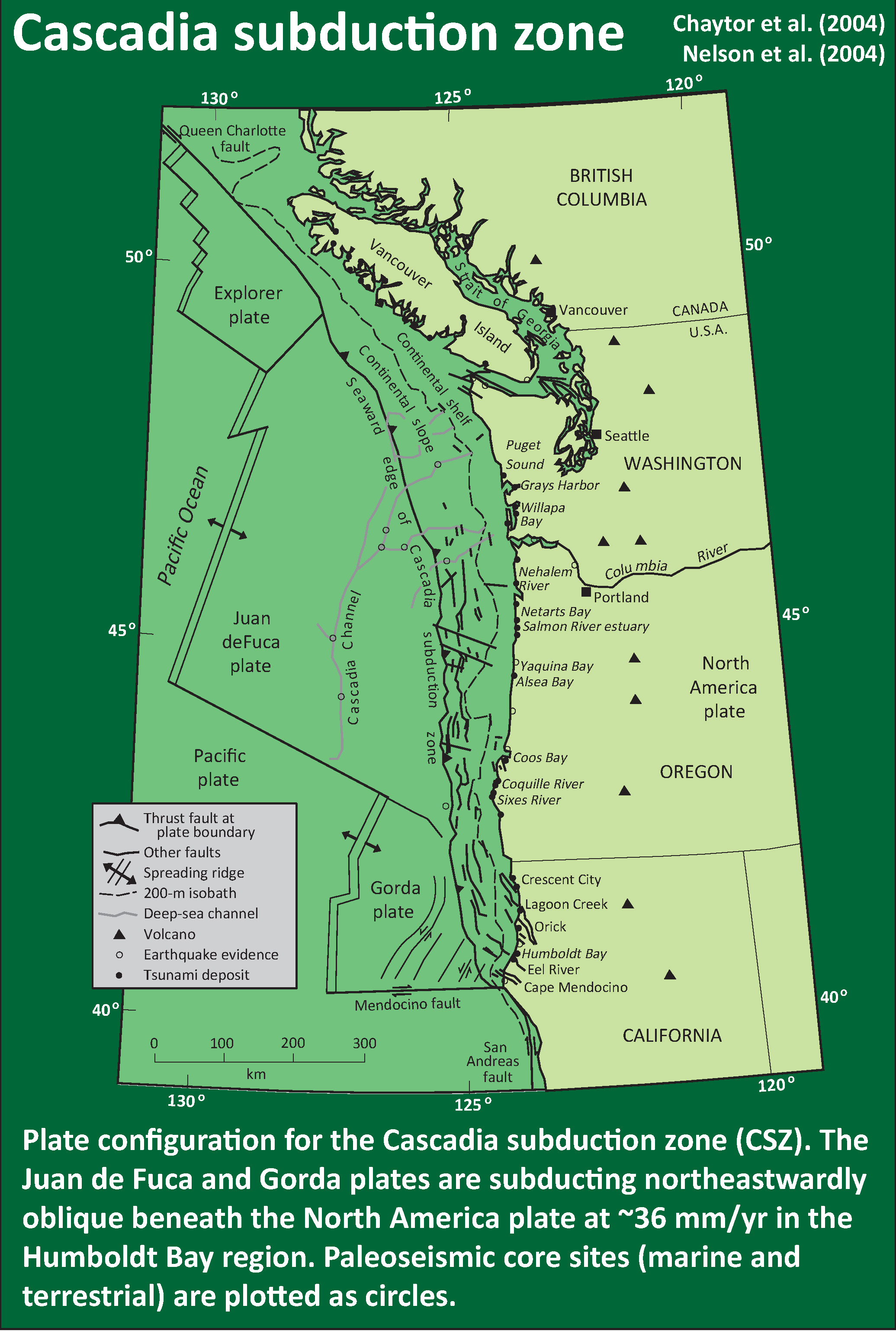
- n the upper left corner is a map of the Cascadia subduction zone (CSZ) and regional tectonic plate boundary faults. This is modified from several sources (Chaytor et al., 2004; Nelson et al., 2004)
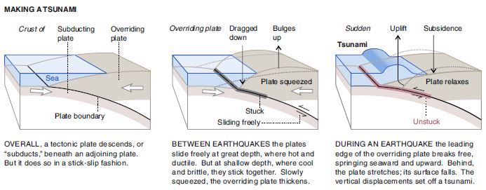
Below the CSZ map is an illustration modified from Plafker (1972). This figure shows how a subduction zone deforms between (interseismic) and during (coseismic) earthquakes. - In the lower right corner is a map that shows a comparison between the USGS Did You Feel It? reports and the USGS Modified Mercalli Intensity shakemap model. This comparison shows that the model is a decent fit for the reports from real people. If you felt the earthquake, please submit a report to the USGS here.
- In the upper right corner I include a larger scale view of seismicity for this area. I highlight the important historic events (e.g. the 1991 Honeydew Earthquake and the 1992 Cape Mendocino Earthquake sequence.
I include some inset figures. Some of the same figures are located in different places on the larger scale map below.
- Here is the map with a month’s seismicity plotted.

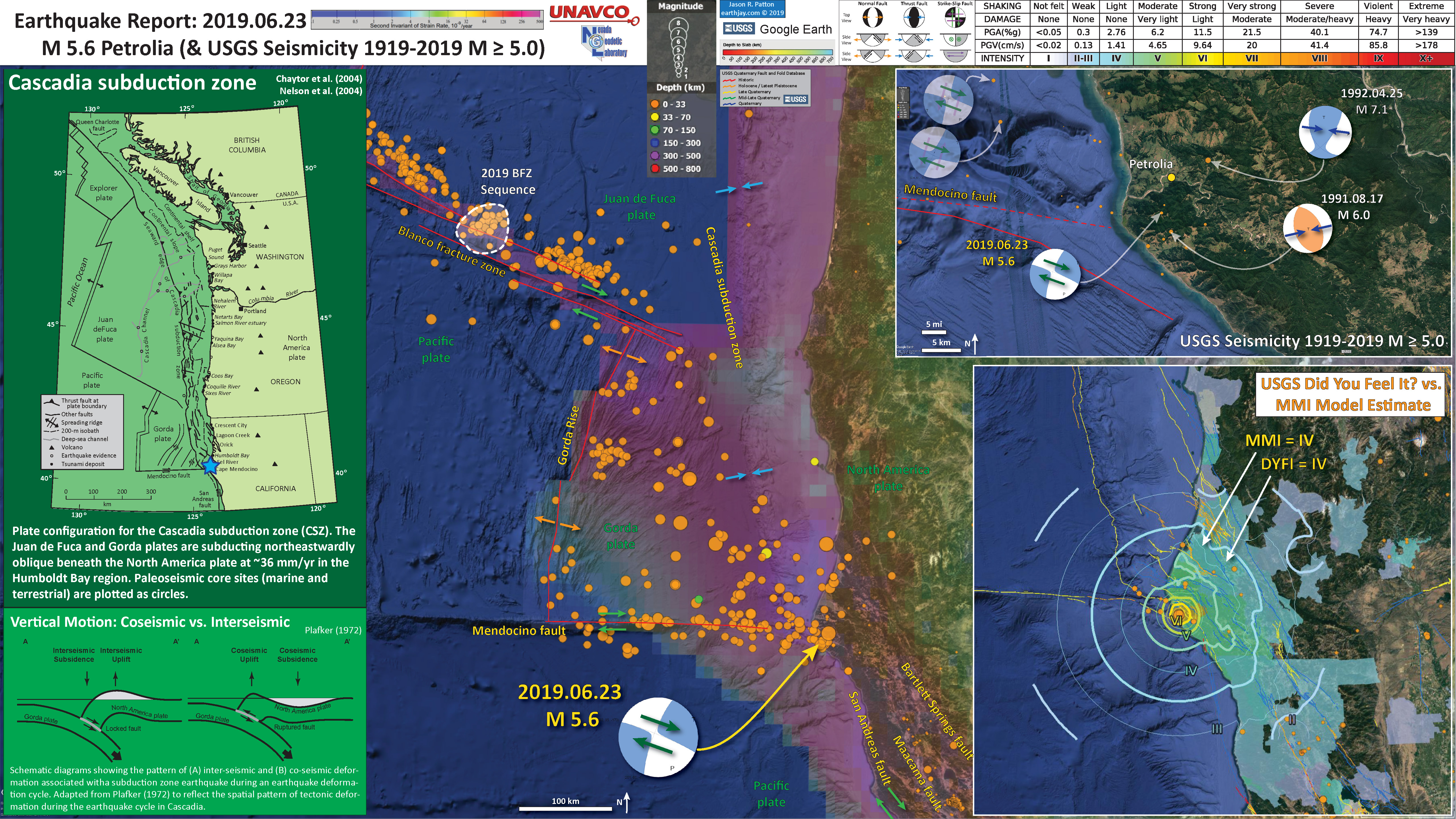
- Here is the map with a century’s seismicity plotted.

- Here is the map with a century’s seismicity plotted along with the Global Strain Map with a 30% transparency.
- Here is the educational interpretive poster from the 1992 Cape Mendocino Earthquake (report here).
- The USGS has been increasing the list of products that are produced in association with their earthquake pages. One of these products is an earthquake forecast (not a prediction as nobody can predict earthquakes yet) that lists the chance of an earthquake with a given magnitude over a certain period of time. The forecast for the M 5.6 earthquake is found here. These forecasts are updated periodically, so the information will change with time. Below is a table where I present the forecast as it was when I checked the page this morning (would be nice if the USGS would produce an easy to read table).
- More earthquakes than usual (called aftershocks) will continue to occur near the mainshock.
- When there are more earthquakes, the chance of a large earthquake is greater which means that the chance of damage is greater.
- The USGS advises everyone to be aware of the possibility of aftershocks, especially when in or around vulnerable structures such as unreinforced masonry buildings.
- This earthquake could be part of a sequence. An earthquake sequence may have larger and potentially damaging earthquakes in the future, so remember to: Drop, Cover, and Hold on.
- According to our forecast, over the next 1 Week there is a < 1 % chance of one or more aftershocks that are larger than magnitude 5.6. It is likely that there will be smaller earthquakes over the next 1 Week, with 0 to 11 magnitude 3 or higher aftershocks. Magnitude 3 and above are large enough to be felt near the epicenter. The number of aftershocks will drop off over time, but a large aftershock can increase the numbers again, temporarily.
- No one can predict the exact time or place of any earthquake, including aftershocks. Our earthquake forecasts give us an understanding of the chances of having more earthquakes within a given time period in the affected area. We calculate this earthquake forecast using a statistical analysis based on past earthquakes.
- Our forecast changes as time passes due to decline in the frequency of aftershocks, larger aftershocks that may trigger further earthquakes, and changes in forecast modeling based on the data collected for this earthquake sequence.
From the USGS:
Be ready for more earthquakes
What we think will happen next
About our earthquake forecasts

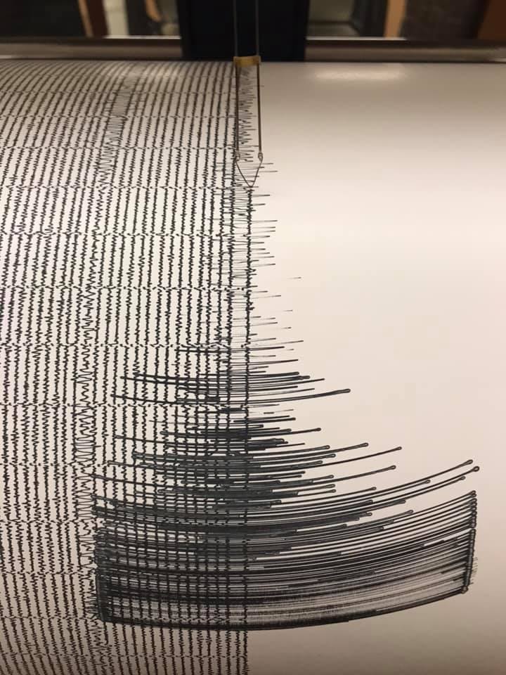
- Gosh, almost forgot to include this photo of the seismic waves recorded on the Humboldt State University Department of Geology Baby Benioff seismometer. Photo Credit: Amanda Admire.
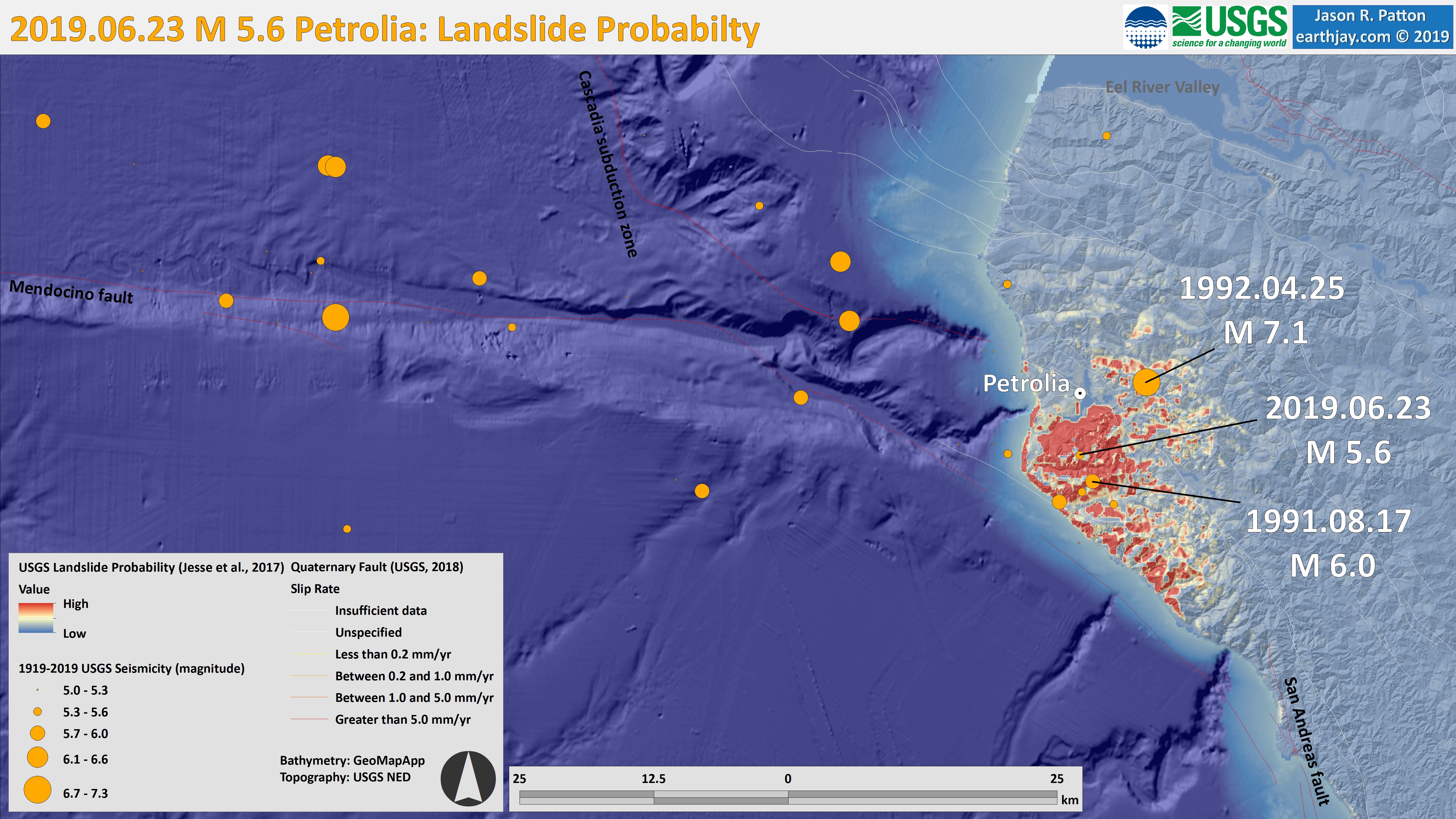
USGS Landslide and Liquefaction Ground Failure data products
- Below I present a series of maps that are intended to address the excellent ‘new’ products included in the USGS earthquake pages: landslide probability and liquefaction susceptibility (a.k.a. the Ground Failure data products).
- First I present the landslide probability model. This is a GIS data product that relates a variety of factors to the probability (the chance of) landslides as triggered by this earthquake. There are a number of assumptions that are made in order to be able to produce this model across such a large region, though this is still of great value (like other aspects from teh USGS, e.g. the PAGER alert). Learn more about all of these Ground Failure products here.
- There are many different ways in which a landslide can be triggered. The first order relations behind slope failure (landslides) is that the “resisting” forces that are preventing slope failure (e.g. the strength of the bedrock or soil) are overcome by the “driving” forces that are pushing this land downwards (e.g. gravity). I spend more time discussing landslides and liquefaction in this recent earthquake report.
- This model, like all landslide computer models, uses similar inputs. I review these here:
- Some information about ground shaking. Often, people use Peak Ground Acceleration, though in the past decade+, it has been recognized that the parameter “Arias Intensity” is a better measure of the energy imparted by the earthquake across the land and seascape. Instead of simply accounting for the peak accelerations, AI integrates the entire energy (duration) during the earthquake. That being said, PGA is a more common parameter that is available for people to use. For example, when I was modeling slope stability for the 2004 Sumatra-Andaman subduction zone earthquake, the only model that was calibrated to observational data were in units of PGA. The first order control to shaking intensity (energy observed at any particular location) is distance to the earthquake fault that slipped.
- Some information about the strength of the materials (e.g. angle of internal friction (the strength) and cohesion (the resistance).
- Information about the slope. Steeper slopes, with all other things being equal, are more likely to fail than are shallower slopes. Think about skiing. Beginners (like me) often choose shallower slopes to ski because they will go down the slope slower, while experts choose steeper slopes.
- Areas that are red are more likely to experience landslides than areas that are colored blue. I include a coarse resolution topographic/bathymetric dataset to help us identify where the mountains are relative to the coastal plain and continental shelf (submarine).
- Landslide ground shaking can change the Factor of Safety in several ways that might increase the driving force or decrease the resisting force. Keefer (1984) studied a global data set of earthquake triggered landslides and found that larger earthquakes trigger larger and more numerous landslides across a larger area than do smaller earthquakes. Earthquakes can cause landslides because the seismic waves can cause the driving force to increase (the earthquake motions can “push” the land downwards), leading to a landslide. In addition, ground shaking can change the strength of these earth materials (a form of resisting force) with a process called liquefaction.
- Sediment or soil strength is based upon the ability for sediment particles to push against each other without moving. This is a combination of friction and the forces exerted between these particles. This is loosely what we call the “angle of internal friction.” Liquefaction is a process by which pore pressure increases cause water to push out against the sediment particles so that they are no longer touching.
- An analogy that some may be familiar with relates to a visit to the beach. When one is walking on the wet sand near the shoreline, the sand may hold the weight of our body generally pretty well. However, if we stop and vibrate our feet back and forth, this causes pore pressure to increase and we sink into the sand as the sand liquefies. Or, at least our feet sink into the sand.
- The liquefaction susceptibility map for the M 5.6 earthquake did not suggest that there would be possibly much liquefaction from this earthquake (probably due to the small magnitude). I discuss liquefaction more in my earthquake report on the 28 September 20018 Sulawesi, Indonesia earthquake, landslide, and tsunami here.
- Here is a map that shows shaking intensity using the MMI scale (mentioned and plotted in the main earthquake poster maps). I present this here in the same format as the ground failure model maps so we can compare these other maps with the ground shaking model (which is a first order control on slope failure).

Other Report Pages
Some Relevant Discussion and Figures
- Here is a map of the Cascadia subduction zone, modified from Nelson et al. (2006). The Juan de Fuca and Gorda plates subduct norteastwardly beneath the North America plate at rates ranging from 29- to 45-mm/yr. Sites where evidence of past earthquakes (paleoseismology) are denoted by white dots. Where there is also evidence for past CSZ tsunami, there are black dots. These paleoseismology sites are labeled (e.g. Humboldt Bay). Some submarine paleoseismology core sites are also shown as grey dots. The two main spreading ridges are not labeled, but the northern one is the Juan de Fuca ridge (where oceanic crust is formed for the Juan de Fuca plate) and the southern one is the Gorda rise (where the oceanic crust is formed for the Gorda plate).
- This figure shows how a subduction zone deforms between (interseismic) and during (coseismic) earthquakes.

- Hemphill-Haley, E., 1995. Diatom evidence for earthquake-induced subsidence and tsunami 300 yr ago in southern coastal Washington in GSA Bulletin, v. 107, p. 367-378.
- Nelson, A.R., Shennan, I., and Long, A.J., 1996. Identifying coseismic subsidence in tidal-wetland stratigraphic sequences at the Cascadia subduction zone of western North America in Journal of Geophysical Research, v. 101, p. 6115-6135.
- Atwater, B.F. and Hemphill-Haley, E., 1997. Recurrence Intervals for Great Earthquakes of the Past 3,500 Years at Northeastern Willapa Bay, Washington in U.S. Geological Survey Professional Paper 1576, Washington D.C., 119 pp.
I have compiled some literature about the CSZ earthquake and tsunami. Here is a short list that might help us learn about what is contained within the core that I collected.
- This figure shows how a subduction zone deforms between (interseismic) and during (coseismic) earthquakes. We also can see how a subduction zone generates a tsunami. Atwater et al., 2005.
- Here is an animation produced by the folks at Cal Tech following the 2004 Sumatra-Andaman subduction zone earthquake. I have several posts about that earthquake here and here. One may learn more about this animation, as well as download this animation here.
- Here is a link to the embedded video below, showing the week-long seismicity in April 1992.
- This is the map used in the animation below. Earthquake epicenters are plotted (some with USGS moment tensors) for this region from 1917-2017 with M ≥ 6.5. I labeled the plates and shaded their general location in different colors.
- I include some inset maps.
- In the upper right corner is a map of the Cascadia subduction zone (Chaytor et al., 2004; Nelson et al., 2004).
- In the upper left corner is a map from Rollins and Stein (2010). They plot epicenters and fault lines involved in earthquakes between 1976 and 2010.

- Here is a link to the embedded video below, showing these earthquakes.
Geologic Fundamentals
- For more on the graphical representation of moment tensors and focal mechanisms, check this IRIS video out:
- Here is a fantastic infographic from Frisch et al. (2011). This figure shows some examples of earthquakes in different plate tectonic settings, and what their fault plane solutions are. There is a cross section showing these focal mechanisms for a thrust or reverse earthquake. The upper right corner includes my favorite figure of all time. This shows the first motion (up or down) for each of the four quadrants. This figure also shows how the amplitude of the seismic waves are greatest (generally) in the middle of the quadrant and decrease to zero at the nodal planes (the boundary of each quadrant).

- Here is another way to look at these beach balls.
The two beach balls show the stike-slip fault motions for the M6.4 (left) and M6.0 (right) earthquakes. Helena Buurman's primer on reading those symbols is here. pic.twitter.com/aWrrb8I9tj
— AK Earthquake Center (@AKearthquake) August 15, 2018
- There are three types of earthquakes, strike-slip, compressional (reverse or thrust, depending upon the dip of the fault), and extensional (normal). Here is are some animations of these three types of earthquake faults. The following three animations are from IRIS.
Strike Slip:
Compressional:
Extensional:
- This is an image from the USGS that shows how, when an oceanic plate moves over a hotspot, the volcanoes formed over the hotspot form a series of volcanoes that increase in age in the direction of plate motion. The presumption is that the hotspot is stable and stays in one location. Torsvik et al. (2017) use various methods to evaluate why this is a false presumption for the Hawaii Hotspot.
- Here is a map from Torsvik et al. (2017) that shows the age of volcanic rocks at different locations along the Hawaii-Emperor Seamount Chain.
- Here is a great tweet that discusses the different parts of a seismogram and how the internal structures of the Earth help control seismic waves as they propagate in the Earth.

A cutaway view along the Hawaiian island chain showing the inferred mantle plume that has fed the Hawaiian hot spot on the overriding Pacific Plate. The geologic ages of the oldest volcano on each island (Ma = millions of years ago) are progressively older to the northwest, consistent with the hot spot model for the origin of the Hawaiian Ridge-Emperor Seamount Chain. (Modified from image of Joel E. Robinson, USGS, in “This Dynamic Planet” map of Simkin and others, 2006.)

Hawaiian-Emperor Chain. White dots are the locations of radiometrically dated seamounts, atolls and islands, based on compilations of Doubrovine et al. and O’Connor et al. Features encircled with larger white circles are discussed in the text and Fig. 2. Marine gravity anomaly map is from Sandwell and Smith.
Today, on #SeismogramSaturday: what are all those strangely-named seismic phases described in seismograms from distant earthquakes? And what do they tell us about Earth’s interior? pic.twitter.com/VJ9pXJFdCy
— Jackie Caplan-Auerbach (@geophysichick) February 23, 2019
- 1700.09.26 M 9.0 Cascadia’s 315th Anniversary 2015.01.26
- 1700.09.26 M 9.0 Cascadia’s 316th Anniversary 2016.01.26 updated in 2017 and 2018
- 1992.04.25 M 7.1 Cape Mendocino 25 year remembrance
- 1992.04.25 M 7.1 Cape Mendocino 25 Year Remembrance Event Page
- Earthquake Information about the CSZ 2015.10.08
- 2018.07.24 M 5.6 Gorda plate
- 2018.03.22 M 4.6/4.7 Gorda plate
- 2017.07.28 M 5.1 Gorda plate
- 2016.09.25 M 5.0 Gorda plate
- 2016.09.25 M 5.0 Gorda plate
- 2016.01.30 M 5.0 Gorda plate
- 2015.12.29 M 4.9 Gorda plate
- 2015.11.18 M 3.2 Gorda plate
- 2014.03.13 M 5.2 Gorda Rise
- 2014.03.09 M 6.8 Gorda plate p-1
- 2014.03.23 M 6.8 Gorda plate p-2
- 2018.08.22 M 6.2 Blanco fracture zone
- 2018.07.29 M 5.3 Blanco fracture zone
- 2015.06.01 M 5.8 Blanco fracture zone p-1
- 2015.06.01 M 5.8 Blanco fracture zone p-2 (animations)
- 2018.01.25 M 5.8 Mendocino fault
- 2017.09.22 M 5.7 Mendocino fault
- 2016.12.08 M 6.5 Mendocino fault, CA
- 2016.12.08 M 6.5 Mendocino fault, CA Update #1
- 2016.12.05 M 4.3 Petrolia CA
- 2016.10.27 M 4.1 Mendocino fault
- 2016.09.03 M 5.6 Mendocino
- 2016.01.02 M 4.5 Mendocino fault
- 2015.11.01 M 4.3 Mendocino fault
- 2015.01.28 M 5.7 Mendocino fault
- 2019.06.23 M 5.6 Petrolia
- 2017.03.06 M 4.0 Cape Mendocino
- 2016.11.02 M 3.6 Oregon
- 2016.01.07 M 4.2 NAP(?)
- 2015.10.29 M 3.4 Bayside
- 2018.10.22 M 6.8 Explorer plate
- 2017.01.07 M 5.7 Explorer plate
- 2016.03.19 M 5.2 Explorer plate
- 2017.06.11 M 3.5 Gorda or NAP?
- 2016.07.21 M 4.7 Gorda or NAP? p-1
- 2016.07.21 M 4.7 Gorda or NAP? p-2
Cascadia subduction zone
General Overview
Earthquake Reports
Gorda plate
Blanco fracture zone
Mendocino fault
Mendocino triple junction
North America plate
Explorer plate
Uncertain
Social Media
- Atwater, B.F., Musumi-Rokkaku, S., Satake, K., Tsuju, Y., Eueda, K., and Yamaguchi, D.K., 2005. The Orphan Tsunami of 1700—Japanese Clues to a Parent Earthquake in North America, USGS Professional Paper 1707, USGS, Reston, VA, 144 pp.
- Goldfinger, C., Nelson, C.H., Morey, A., Johnson, J.E., Gutierrez-Pastor, J., Eriksson, A.T., Karabanov, E., Patton, J., Gràcia, E., Enkin, R., Dallimore, A., Dunhill, G., and Vallier, T., 2012 a. Turbidite Event History: Methods and Implications for Holocene Paleoseismicity of the Cascadia Subduction Zone, USGS Professional Paper # 1661F. U.S. Geological Survey, Reston, VA, 184 pp.
- Dengler, L.A., and McPherson, R.C., 1993. The 17 August 1991 Honeydew Earthquake, North Coast California: A Case for Revising the Modified Mercalli Scale in Sparsely Populated Areas in BSSA, v. 83, no. 4, pp. 1081-1094
- Frisch, W., Meschede, M., Blakey, R., 2011. Plate Tectonics, Springer-Verlag, London, 213 pp.
- Hayes, G., 2018, Slab2 – A Comprehensive Subduction Zone Geometry Model: U.S. Geological Survey data release, https://doi.org/10.5066/F7PV6JNV.
- Holt, W. E., C. Kreemer, A. J. Haines, L. Estey, C. Meertens, G. Blewitt, and D. Lavallee (2005), Project helps constrain continental dynamics and seismic hazards, Eos Trans. AGU, 86(41), 383–387, , https://doi.org/10.1029/2005EO410002. /li>
- Kreemer, C., J. Haines, W. Holt, G. Blewitt, and D. Lavallee (2000), On the determination of a global strain rate model, Geophys. J. Int., 52(10), 765–770.
- Kreemer, C., W. E. Holt, and A. J. Haines (2003), An integrated global model of present-day plate motions and plate boundary deformation, Geophys. J. Int., 154(1), 8–34, , https://doi.org/10.1046/j.1365-246X.2003.01917.x.
- Kreemer, C., G. Blewitt, E.C. Klein, 2014. A geodetic plate motion and Global Strain Rate Model in Geochemistry, Geophysics, Geosystems, v. 15, p. 3849-3889, https://doi.org/10.1002/2014GC005407.
- McCrory, P.A., 2000, Upper plate contraction north of the migrating Mendocino triple junction, northern California: Implications for partitioning of strain: Tectonics, v. 19, p. 11441160.
- McCrory, P. A., Blair, J. L., Oppenheimer, D. H., and Walter, S. R., 2006, Depth to the Juan de Fuca slab beneath the Cascadia subduction margin; a 3-D model for sorting earthquakes U. S. Geological Survey
- Meyer, B., Saltus, R., Chulliat, a., 2017. EMAG2: Earth Magnetic Anomaly Grid (2-arc-minute resolution) Version 3. National Centers for Environmental Information, NOAA. Model. https://doi.org/10.7289/V5H70CVX
- Müller, R.D., Sdrolias, M., Gaina, C. and Roest, W.R., 2008, Age spreading rates and spreading asymmetry of the world’s ocean crust in Geochemistry, Geophysics, Geosystems, 9, Q04006, https://doi.org/10.1029/2007GC001743
- Nelson, A.R., Kelsey, H.M., Witter, R.C., 2006. Great earthquakes of variable magnitude at the Cascadia subduction zone. Quaternary Research 65, 354-365.
- Oppenheimer, D., Beroza, G., Carver, G., Dengler, L., Eaton, J., Gee, L., Gonzalez, F., Jayko, A., Ki., W.H., Lisowski, M., Magee, M., Marshall, G., Murray, M., McPherson, R., Romanowicz, B., Satake, K., Simpson, R., Somerille, P., Stein, R., and Valentine, D., The Cape Mendocino, California, Earthquakes of April, 1992: Subduction at the Triple Junction in Science, v. 261, no. 5120, p. 433-438.
- Patton, J. R., Goldfinger, C., Morey, A. E., Romsos, C., Black, B., Djadjadihardja, Y., and Udrekh, 2013. Seismoturbidite record as preserved at core sites at the Cascadia and Sumatra–Andaman subduction zones, Nat. Hazards Earth Syst. Sci., 13, 833-867, doi:10.5194/nhess-13-833-2013, 2013.
- Plafker, G., 1972. Alaskan earthquake of 1964 and Chilean earthquake of 1960: Implications for arc tectonics in Journal of Geophysical Research, v. 77, p. 901-925.
- Rollins, J.C. and Stein, R.S., 2010. Coulomb stress interactions among M ≥ 5.9 earthquakes in the Gorda deformation zone and on the Mendocino Fault Zone, Cascadia subduction zone, and northern San Andreas Fault: Journal of Geophysical Research, v. 115, B12306, doi:10.1029/2009JB007117, 2010.
- Stein, R.S., Marshall, G.A., Murray, M.H., Balazs, E., Carver, G.A., Dunklin, T.A>, McLaughlin, R.J., Cyr, K., and Jayko, A., 1993. Permanent Ground Movement Associate with the 1992 M=7 Cape Mendocino, California, Earthquake: Implications for Damage to Infrastructure and Hazards to navigation, U.S. Geological Survey Open-File Report 93-383.
- Wang, K., Wells, R., Mazzotti, S., Hyndman, R. D., and Sagiya, T., 2003, A revised dislocation model of interseismic deformation of the Cascadia subduction zone Journal of Geophysical Research, B, Solid Earth and Planets v. 108, no. 1.
References:
Return to the Earthquake Reports page.
Mind if I grab an occasional screenshot or graphic from your site for tweets, Jay? The text will always include the permalink back here for attribution. The relevant tweets are reports of seismic activity sometimes seen on the Oroville Dam seismographs, usu. ORV, with my meager attempts to identify the source – earthquake, aliens, dam failure, etc.
-
that’s great! the images can be downloaded by clicking on them… cheers