
The 25 April 1992 M 7.1 earthquake was a wake up call for many, like all large magnitude earthquakes are.
I have some updated posters as of April 2021 (see below).
Here is my personal story.
I was driving my girlfriend’s car (Jen Guevara) with her and some housemates up to attend a festival at Redwood Park in Arcata. She lived in the old blue house at the base of the bridge abutment on the southwest side of HWY 101 as it crosses Mad River. The house burned down a couple of years ago, but these memories remain. We were driving along St. Louis and about to turn east to cross the 101 towards LK Wood. The car moved left and right. I pulled over as I thought we might have just gotten a flat tire. I got out, inspected the wheels, and there was no flat. We returned to our journey. When we arrived at the park, everyone was talking about how the redwood trees were flopping around like wet spaghetti during the earthquake. I then looked back in my memory and realized that, at the lumber mill that I had parked by when I got the imaginary flat tire, there were tall stacks of milled lumber flopping around. I had dismissed it that they were blowing in the wind. Silly me.
Later that night, I was at a reggae concert at the Old Creamery Building in Arcata. At some point, the lights flickered off and on. I figured that someone had accidentally brushed up against the light switch on the wall. BUT, this was the first of two large aftershocks.
Even later that night, actually the following morning, I was laying in bed with Jen. The house typically shook when large semi trucks crossed the 101 bridge. However, this time, the shaking had a much longer duration. This was the second of the two major aftershocks. I finally recognized this earthquake as an earthquake and not something else. To my credit, I was dancing during the first major aftershock.
- 1992-04-25 18:06:05 UTC 40.335°N 124.229°W 9.9 km depth M 7.2
- 1992-04-26 07:41:40 UTC 40.433°N 124.566°W 18.8 km depth M 6.5
- 1992-04-26 11:18:25 UTC 40.383°N 124.555°W 21.7 km depth M 6.6
Here is the USGS website for these three large earthquakes.
- California Geological Survey Earthquake and Tsunami Website
- California Geological Survey “A Geological Adventure”
- Berkeley Seismo Blog
- Northcoast Journal (read some other personal stories)
- NOAA
Here are some additional web pages that cover this earthquake.
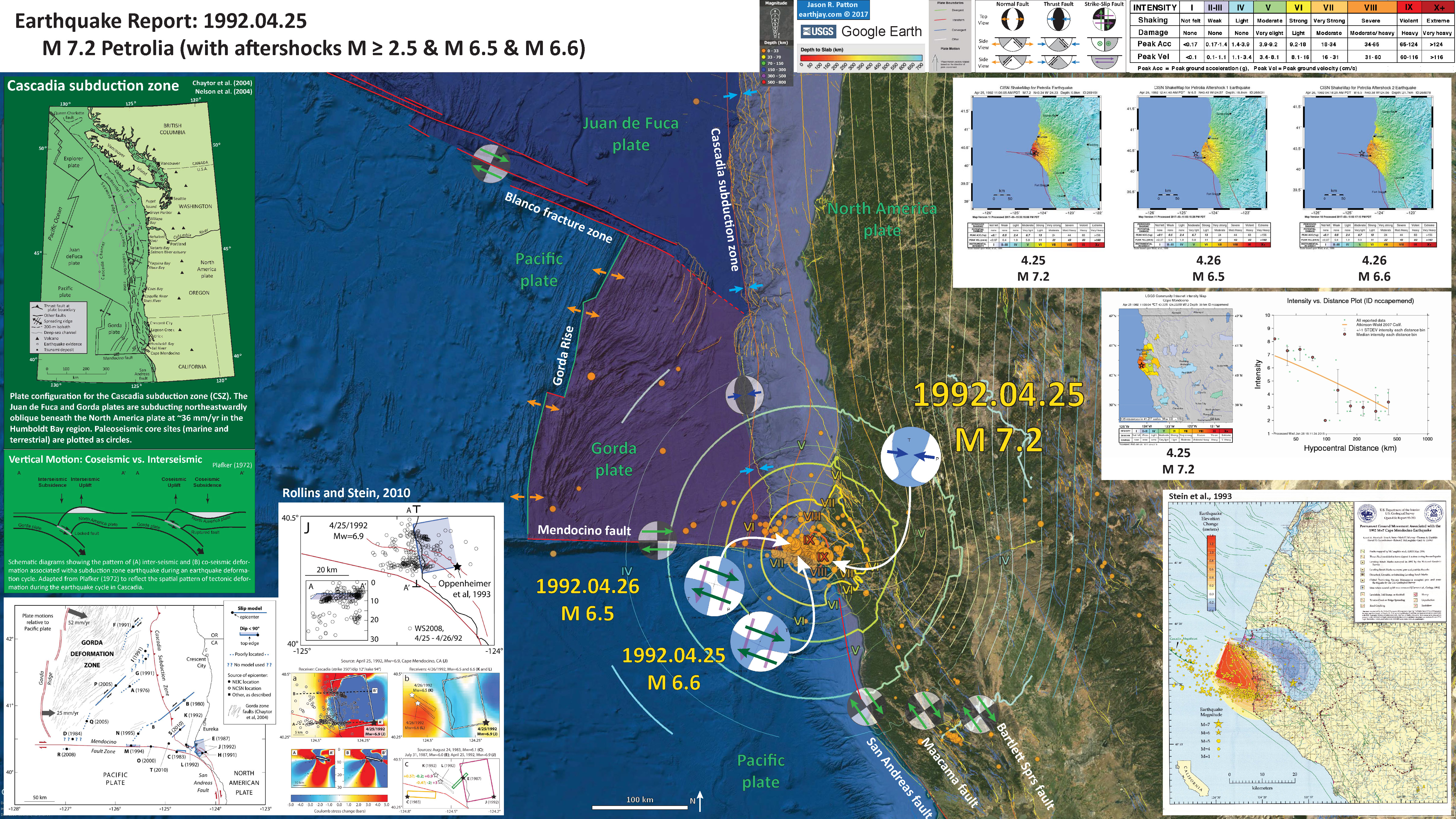
Below is my interpretive poster for this earthquake.
I plot the seismicity for a week beginning April 25, 1992, with color representing depth and diameter representing magnitude (see legend)..
- I placed a moment tensor / focal mechanism legend on the poster. There is more material from the USGS web sites about moment tensors and focal mechanisms (the beach ball symbols). Both moment tensors and focal mechanisms are solutions to seismologic data that reveal two possible interpretations for fault orientation and sense of motion. One must use other information, like the regional tectonics, to interpret which of the two possibilities is more likely.
- I also include the shaking intensity contours on the map. These use the Modified Mercalli Intensity Scale (MMI; see the legend on the map). This is based upon a computer model estimate of ground motions, different from the “Did You Feel It?” estimate of ground motions that is actually based on real observations. The MMI is a qualitative measure of shaking intensity. More on the MMI scale can be found here and here. This is based upon a computer model estimate of ground motions, different from the “Did You Feel It?” estimate of ground motions that is actually based on real observations.
- I include the slab contours plotted (McCrory et al., 2012), which are contours that represent the depth to the subduction zone fault. These are mostly based upon seismicity. The depths of the earthquakes have considerable error and do not all occur along the subduction zone faults, so these slab contours are simply the best estimate for the location of the fault.
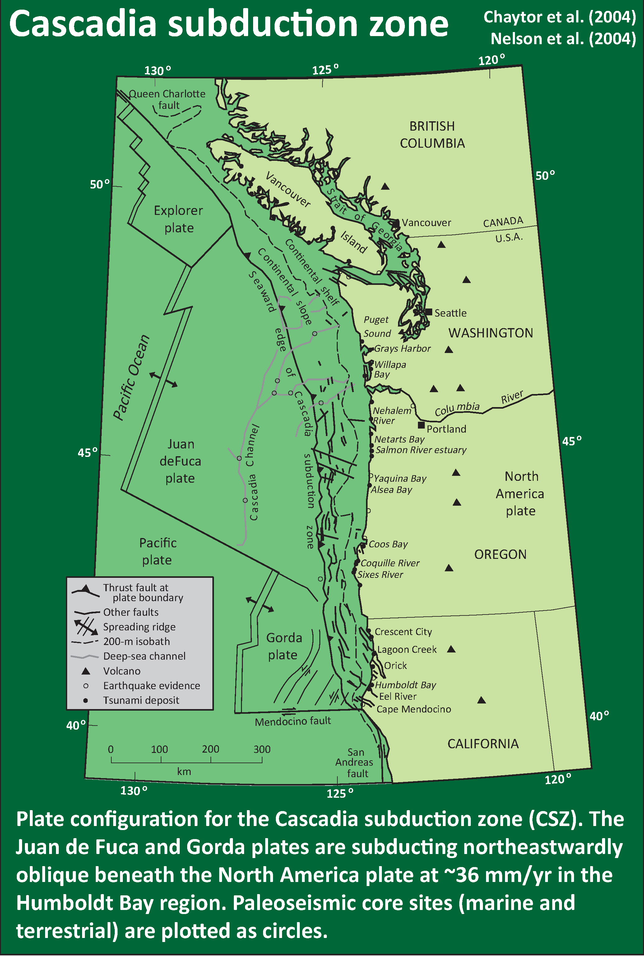
- In the upper left corner is a map of the Cascadia subduction zone (CSZ) and regional tectonic plate boundary faults. This is modified from several sources (Chaytor et al., 2004; Nelson et al., 2004)
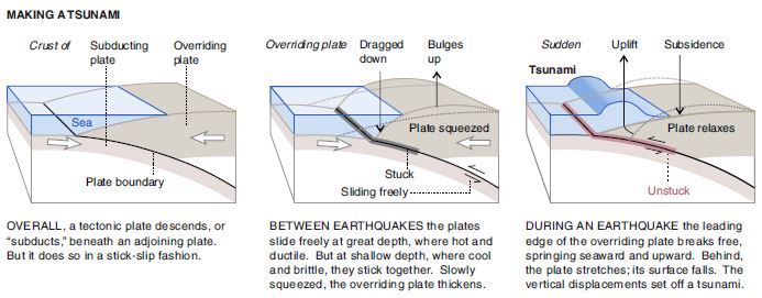
- Below the CSZ map is an illustration modified from Plafker (1972). This figure shows how a subduction zone deforms between (interseismic) and during (coseismic) earthquakes.
- In the upper left corner is a figure from Rollins and Stein (2010). In their paper they discuss how static coulomb stress changes from earthquakes may impart (or remove) stress from adjacent crust/faults. To the right of this map are two panels. The upper panel shows the location and orientation of the fault plane used by Rollins and Stein (2010) to model potential changes in coulomb stress following the 1992 M 7.2 earthquake. The Lower panel shows the results from this modeling.
- In the lower right corner is the map from Stein et al. (1993). This map shows an estimate of coseismic vertical ground motion induced by the 1992 earthquake sequence.
- In the upper right corner is a series of USGS shakemaps. These plot intensity using the MMI scale.
- Below the shakemaps is the “Did You Feel It?” map and attenuation relation plot.
I include some inset figures in the poster.
Below is my updated interpretive poster for this earthquake.
- In the upper left corner is a small scale map that shows the tectonic plates and their boundaries, along with USGS NEIC seismicity from 1921-2021 for earthquakes M > 6.5
- In the upper right corner is a series of 4 panels highlighting earthquake intensity for the 3 main events in this sequence.
- The 3 panels on the right show the Modified Mercalli Intensity (MMI) scale shaking intensity for the 7.2, 6.6, and 6.5 earthquakes. These are based on computer models that correlate MMI with distance from the earthquake.
- The panel on the left is a larger scale map that shows the MMI contours for the 7.2 earthquake. I also plot the USGS “Did You Feel It?” results. These are data compiled from observations people made and reported to the USGS. Read more about the DYFI program here.
- The plot in the bottom center-left shows both of these data: the USGS modeled intensities and the USGS DYFI intensities. Note how the intensity gets lesser with distance from the earthquake.
- The lower right corner has two maps which are “Ground Failure” products from the USGS for this earthquake. Read more about the USGS ground failure products here. I explain these two products in greater detail below.
- The map on the right shows the probability of (chance of) landslides to have been triggered by the M 7.2 earthquake shaking.
- The map on the left shows the susceptibility for (chance for) liquefaction to have been generated by the M 7.2 earthquake shaking.
- Above the Ground Failure maps is a larger scale view of the aftershocks from the Cape Mendocino Earthquake. Technically, many of these events are not aftershocks, but earthquakes on different faults than the M 7.2 source fault. These are earthquakes triggered by the stress changes following the 7.2 earthquake. The two second largest events (M 6.6 and 6.5) are triggered events on NW striking faults in the Gorda plate. More on these events in an upcoming paper. Stay tuned.
I include some inset figures in the poster.

Here is a fantastic video about the Mendocino triple junction from our local earthquake expert Thomas Dunklin.
Shaking Intensity and Potential for Ground Failure
- Below are a series of maps that show the shaking intensity and potential for landslides and liquefaction. These are all USGS data products.
- Below is the liquefaction susceptibility and landslide probability map (Jessee et al., 2017; Zhu et al., 2017). Please head over to that report for more information about the USGS Ground Failure products (landslides and liquefaction). Basically, earthquakes shake the ground and this ground shaking can cause landslides. We can see that there is a high probability for landslides. This makes sense as the lower limit for earthquake triggered landslides is magnitude M 5.5 (from Keefer 1984).
- I use the same color scheme that the USGS uses on their website. Note how the areas that are more likely to have experienced earthquake induced liquefaction are in the valleys. Learn more about how the USGS prepares these model results here.
There are many different ways in which a landslide can be triggered. The first order relations behind slope failure (landslides) is that the “resisting” forces that are preventing slope failure (e.g. the strength of the bedrock or soil) are overcome by the “driving” forces that are pushing this land downwards (e.g. gravity). The ratio of resisting forces to driving forces is called the Factor of Safety (FOS). We can write this ratio like this:
FOS = Resisting Force / Driving Force
When FOS > 1, the slope is stable and when FOS < 1, the slope fails and we get a landslide. The illustration below shows these relations. Note how the slope angle α can take part in this ratio (the steeper the slope, the greater impact of the mass of the slope can contribute to driving forces). The real world is more complicated than the simplified illustration below.

Landslide ground shaking can change the Factor of Safety in several ways that might increase the driving force or decrease the resisting force. Keefer (1984) studied a global data set of earthquake triggered landslides and found that larger earthquakes trigger larger and more numerous landslides across a larger area than do smaller earthquakes. Earthquakes can cause landslides because the seismic waves can cause the driving force to increase (the earthquake motions can “push” the land downwards), leading to a landslide. In addition, ground shaking can change the strength of these earth materials (a form of resisting force) with a process called liquefaction.
Sediment or soil strength is based upon the ability for sediment particles to push against each other without moving. This is a combination of friction and the forces exerted between these particles. This is loosely what we call the “angle of internal friction.” Liquefaction is a process by which pore pressure increases cause water to push out against the sediment particles so that they are no longer touching.
An analogy that some may be familiar with relates to a visit to the beach. When one is walking on the wet sand near the shoreline, the sand may hold the weight of our body generally pretty well. However, if we stop and vibrate our feet back and forth, this causes pore pressure to increase and we sink into the sand as the sand liquefies. Or, at least our feet sink into the sand.
Below is a diagram showing how an increase in pore pressure can push against the sediment particles so that they are not touching any more. This allows the particles to move around and this is why our feet sink in the sand in the analogy above. This is also what changes the strength of earth materials such that a landslide can be triggered.

Below is a diagram based upon a publication designed to educate the public about landslides and the processes that trigger them (USGS, 2004). Additional background information about landslide types can be found in Highland et al. (2008). There was a variety of landslide types that can be observed surrounding the earthquake region. So, this illustration can help people when they observing the landscape response to the earthquake whether they are using aerial imagery, photos in newspaper or website articles, or videos on social media. Will you be able to locate a landslide scarp or the toe of a landslide? This figure shows a rotational landslide, one where the land rotates along a curvilinear failure surface.


The Cascadia subduction zone
- Here is a map of the Cascadia subduction zone, modified from Nelson et al. (2006). The Juan de Fuca and Gorda plates subduct norteastwardly beneath the North America plate at rates ranging from 29- to 45-mm/yr. Sites where evidence of past earthquakes (paleoseismology) are denoted by white dots. Where there is also evidence for past CSZ tsunami, there are black dots. These paleoseismology sites are labeled (e.g. Humboldt Bay). Some submarine paleoseismology core sites are also shown as grey dots. The two main spreading ridges are not labeled, but the northern one is the Juan de Fuca ridge (where oceanic crust is formed for the Juan de Fuca plate) and the southern one is the Gorda rise (where the oceanic crust is formed for the Gorda plate).
- This figure shows how a subduction zone deforms between (interseismic) and during (coseismic) earthquakes.

- Hemphill-Haley, E., 1995. Diatom evidence for earthquake-induced subsidence and tsunami 300 yr ago in southern coastal Washington in GSA Bulletin, v. 107, p. 367-378.
- Nelson, A.R., Shennan, I., and Long, A.J., 1996. Identifying coseismic subsidence in tidal-wetland stratigraphic sequences at the Cascadia subduction zone of western North America in Journal of Geophysical Research, v. 101, p. 6115-6135.
- Atwater, B.F. and Hemphill-Haley, E., 1997. Recurrence Intervals for Great Earthquakes of the Past 3,500 Years at Northeastern Willapa Bay, Washington in U.S. Geological Survey Professional Paper 1576, Washington D.C., 119 pp.
I have compiled some literature about the CSZ earthquake and tsunami. Here is a short list that might help us learn about what is contained within the core that I collected.
- This figure shows how a subduction zone deforms between (interseismic) and during (coseismic) earthquakes. We also can see how a subduction zone generates a tsunami. Atwater et al., 2005.
- Here is an animation produced by the folks at Cal Tech following the 2004 Sumatra-Andaman subduction zone earthquake. I have several posts about that earthquake here and here. One may learn more about this animation, as well as download this animation here.
1992 Cape Mendocino Earthquake and Tsunami
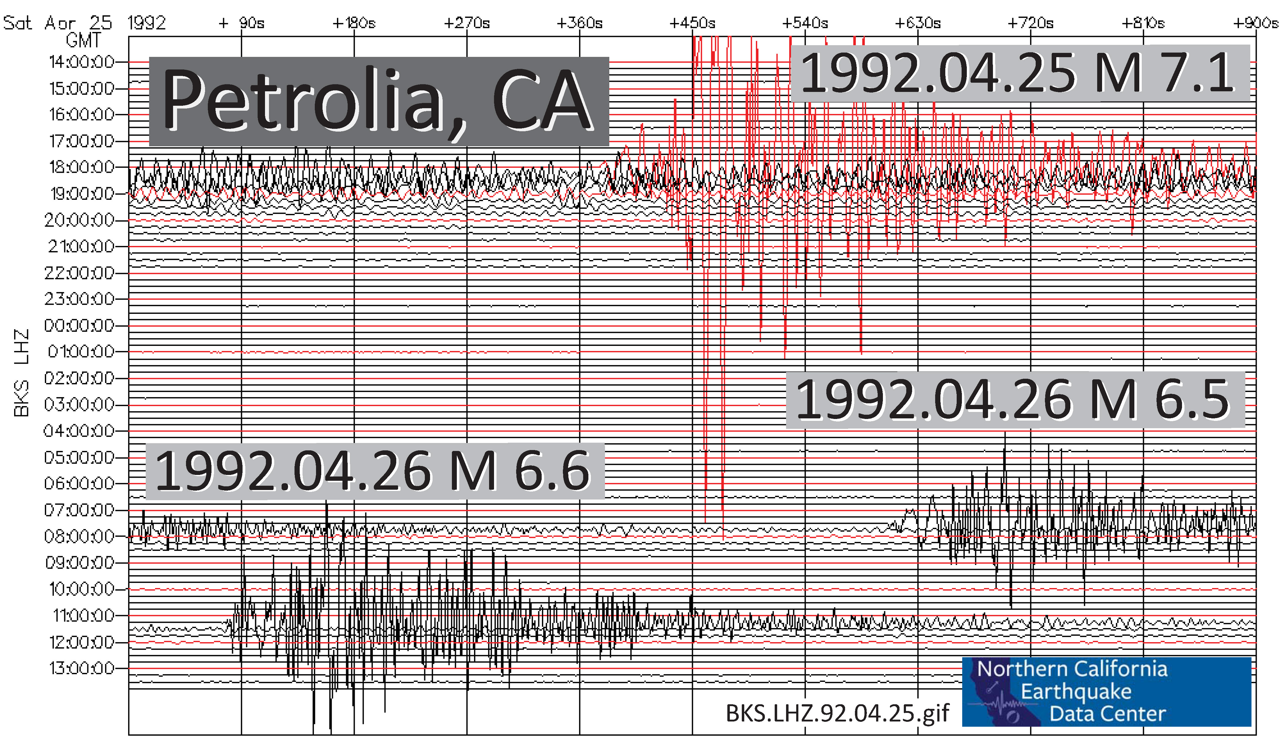
- Here is a link to the embedded video below, showing the week-long seismicity in April 1992.
- Following the earthquake, there was lots of work done by local geologists, along with help from those visiting from out of the area. One of the projects included the measurement and modeling of the ground deformation related to the earthquake. The measurements consistend of a first order survey of benchmarks, along with Global Positioning System measurements at GPS monuments. The results from these analyses were presented in a U.S. Geological Survey Open-File Report 93-383 (Stein et al., 1993). Below is a map that shows a modeled estimate of the surface deformation associated with this earthquake.

- Here is a figure from Oppenheimer et al. (1993) that shows the shaking intensity from this earthquake sequence. Below is a colorized version.
- This map shows an alternate model of earthquake ground deformation (Oppenheimer et al, 1993).
- This is a figure that shows the tsunami recorded by tide gages in California, Hawaii, and Oregon (Oppenheimer et al., 1993)


Simplified tectonic map in the vicinity of the Cape Mendocino earthquake sequence. Stars, epicenters of three largest earthquakes; contours, Modified Mercalli intensities (values, Roman numerals) of main shock; open circles, strong motion instrument sites (adjacent numbers give peak horizontal accelerations in g). Abbreviations FT Fortuna; F Ferndale; RD, Rio Dell; S, Scotia; P, Petrolia; H, Honeydew; MF, Mendocino fault; CSZ, seaward edge of Cascadia subduction zone; and SAF, San Andreas fault.

Observed and predicted coseismic displacements for the Cape Mendocino main shock (epicenter located at star).

- Here is a map from Rollins and Stein (2010), showing their interpretations of different historic earthquakes in the region. This was published in response to the Januray 2010 Gorda plate earthquake. The faults are from Chaytor et al. (2004).
- This figure shows the fault plane and aftershocks used in their analysis of the 1992 earthquake sequence.
- This figure shows the change in coulomb stress imparted by the M 7.1 earthquake onto different faults: (a) the CSZ and (b) the faults that were triggered to generate the two main aftershocks.

Tectonic configuration of the Gorda deformation zone and locations and source models for 1976–2010 M ≥ 5.9 earthquakes. Letters designate chronological order of earthquakes (Table 1 and Appendix A). Plate motion vectors relative to the Pacific Plate (gray arrows in main diagram) are from Wilson [1989], with Cande and Kent’s [1995] timescale correction.

Source models for earthquakes 25 April 1992, Mw = 6.9, open circles are from Waldhauser and Schaff ’s [2008] earthquake locations for 25 April 1992 (1806 UTC) to 26 April 1992 (0741 UTC)

(a) Coulomb stress changes imparted by the 1992 Mw = 6.9 Cape Mendocino earthquake (J) to the Cascadia subduction zone. Calculation depth is 8 km. Open circles are Waldhauser and Schaff [2008] earthquake locations for 25 April 1992 to 2 May 1992, 0–15 km depth. Seismicity data were cut off at 15 km depth to prevent interference from aftershocks of K and L. Cross section A‐A′ includes seismicity between 40.24°N and 40.36°N. Cross section B‐B′ includes seismicity between 40.36°N and 40.48°N. (b) Coulomb stress changes imparted by the 1992 Mw = 6.9 earthquake (J) to Mw = 6.5 and Mw = 6.6 shocks the next day (K and L). Stress change is resolved on the average of the orientations of K and L (strike 127°/dip 90°/rake 180°). Calculation depth is 21.5 km. (c) Calculated Coulomb stress changes imparted by M ≥ 5.9 shocks in 1983, 1987, and 1992 (C, E, and J) to the epicenters of K and L. The series of three colored numbers represent stress changes imparted by C, E, and J, respectively.
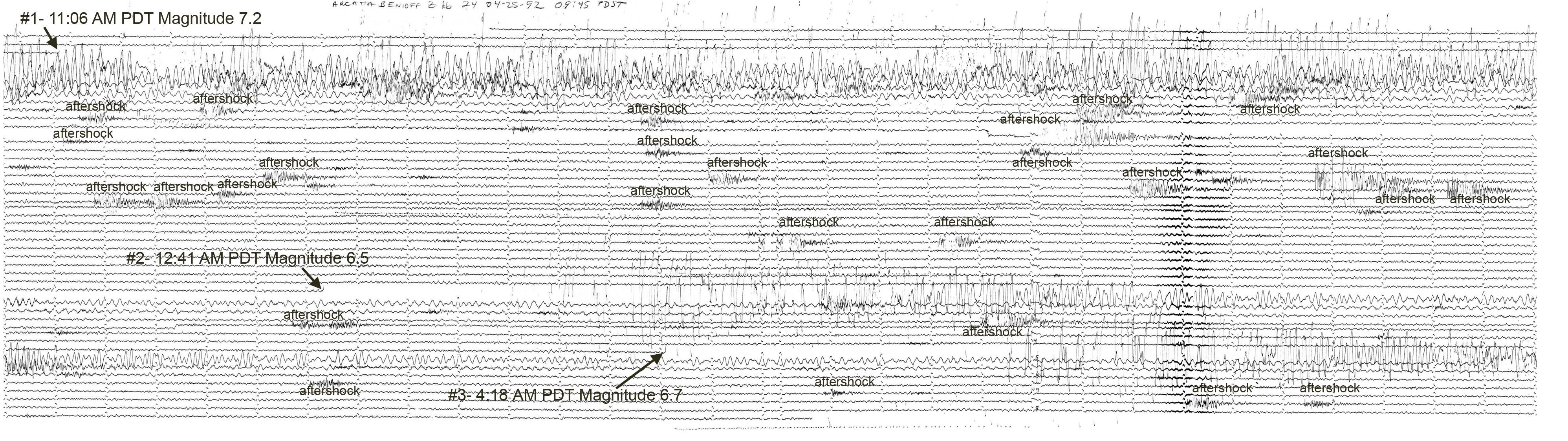
- Here is a plot of the seismograms from the NCEDC.
- Here is the seismogram as recorded at the HSU Dept. of Geology’s seismometer. Here is a link to an unlabeled seismograph.
Below is an updated interpretive poster for this earthquake sequence that focuses on the mechanisms.
- I include the plot of tide gage data from Oppenheimer et al. (1993). These data are not in digital format, but are preserved in paper format. I hope to get some funding to head back to the east coast and scan the paper records to digitize them.
- Note that the color format for the seismicity is based on depth. There are lots of events in the North America plate (see the green dots on the eastern end of the plot. There are also lots of Gorda plate and Mendocino fault events (the deeper events on the western side of the plot).
- Look at the different types of earthquakes. What can you conclude about this sequence?

- 1922.01.31 13:17 M 7.3
- 1923.01.22 09:04 M 6.9
- 1934-07-06 22:48 M 6.7
- 1941-02-09 09:44 M 6.8
- 1949-03-24 20:56 M 6.5
- 1954-11-25 11:16 M 6.8
- 1954-12-21 19:56 M 6.6
- 1980-11-08 10:27 M 7.2
- 1984-09-10 03:14 M 6.7
- 1984-09-10 03:14 M 6.6
- 1991-07-13 02:50 M 6.9
- 1991-08-17 22:17 M 7.0
- 1992-04-25 18:06 M 7.2
- 1992-04-26 07:41 M 6.5
- 1992-04-26 11:18 M 6.6
- 1994-09-01 15:15 M 7.0
- 1995-02-19 04:03 M 6.6
- 2005-06-15 02:50 M 7.2
- 2005-06-17 06:21 M 6.6
- 2010-01-10 00:27 M 6.5
- 2014-03-10 05:18 M 6.8
- 2016-12-08 14:49 M 6.5
Here is the USGS website for all the earthquakes in this region from 1917-2017 with M ≥ 6.5.
- This is the map used in the animation below. Earthquake epicenters are plotted (some with USGS moment tensors) for this region from 1917-2017 with M ≥ 6.5. I labeled the plates and shaded their general location in different colors.
- I include some inset maps.
- In the upper right corner is a map of the Cascadia subduction zone (Chaytor et al., 2004; Nelson et al., 2004).
- In the upper left corner is a map from Rollins and Stein (2010). They plot epicenters and fault lines involved in earthquakes between 1976 and 2010.

- Here is a link to the embedded video below, showing these earthquakes.
- Cascadia’s 315th Anniversary 2015.01.26
- Cascadia’s 316th Anniversary 2016.01.26
- Earthquake Information about the CSZ 2015.10.08
- 2016.09.25 M 5.0 Gorda plate
- 2016.09.25 M 5.0 Gorda plate
- 2016.07.21 M 4.7 Gorda plate p-1
- 2016.07.21 M 4.7 Gorda plate p-2
- 2016.01.30 M 5.0 Gorda plate
- 2015.12.29 M 4.9 Gorda plate
- 2015.11.18 M 3.2 Gorda plate
- 2014.03.13 M 5.2 Gorda Rise
- 2014.03.09 M 6.8 Gorda plate p-1
- 2014.03.23 M 6.8 Gorda plate p-2
- 2015.06.01 M 5.8 Blanco fracture zone p-1
- 2015.06.01 M 5.8 Blanco fracture zone p-2 (animations)
- 2016.12.08 M 6.5 Mendocino fault, CA
- 2016.12.08 M 6.5 Mendocino fault, CA Update #1
- 2016.12.05 M 4.3 Petrolia CA
- 2016.10.27 M 4.1 Mendocino fault
- 2016.09.03 M 5.6 Mendocino
- 2016.01.02 M 4.5 Mendocino fault
- 2015.11.01 M 4.3 Mendocino fault
- 2015.01.28 M 5.7 Mendocino fault
- 2017.03.06 M 4.0 Cape Mendocino
- 2016.11.02 M 3.6 Oregon
- 2016.01.07 M 4.2 NAP(?)
- 2015.10.29 M 3.4 Bayside
- 2017.01.07 M 5.7 Explorer plate
- 2016.03.19 M 5.2 Explorer plate
Cascadia subduction zone
General Overview
Earthquake Reports
Gorda plate
Blanco fracture zone
Mendocino fault
Mendocino triple junction
North America plate
Explorer plate
- There are three types of earthquakes, strike-slip, compressional (reverse or thrust, depending upon the dip of the fault), and extensional (normal). Here is are some animations of these three types of earthquake faults. Many of the earthquakes people are familiar with in the Mendocino triple junction region are either compressional or strike slip. The following three animations are from IRIS.
- Strike Slip:
- Compressional:
- Extensional:
- Here is a primer that helps people learn how to interpret focal mechanisms and moment tensors. Moment tensors are calculated differently from focal mechanisms, but the interpretation of their graphical solution is similar. This is from the USGS.
- For more on the graphical representation of moment tensors and focal mechnisms, check this IRIS video out:
References
- Atwater, B.F., Musumi-Rokkaku, S., Satake, K., Tsuju, Y., Eueda, K., and Yamaguchi, D.K., 2005. The Orphan Tsunami of 1700—Japanese Clues to a Parent Earthquake in North America, USGS Professional Paper 1707, USGS, Reston, VA, 144 pp.
- Goldfinger, C., Nelson, C.H., Morey, A., Johnson, J.E., Gutierrez-Pastor, J., Eriksson, A.T., Karabanov, E., Patton, J., Gràcia, E., Enkin, R., Dallimore, A., Dunhill, G., and Vallier, T., 2012 a. Turbidite Event History: Methods and Implications for Holocene Paleoseismicity of the Cascadia Subduction Zone, USGS Professional Paper # 1661F. U.S. Geological Survey, Reston, VA, 184 pp.
- McCrory, P.A., 2000, Upper plate contraction north of the migrating Mendocino triple junction, northern California: Implications for partitioning of strain: Tectonics, v. 19, p. 11441160.
- McCrory, P. A., Blair, J. L., Oppenheimer, D. H., and Walter, S. R., 2006, Depth to the Juan de Fuca slab beneath the Cascadia subduction margin; a 3-D model for sorting earthquakes U. S. Geological Survey
- Nelson, A.R., Kelsey, H.M., Witter, R.C., 2006. Great earthquakes of variable magnitude at the Cascadia subduction zone. Quaternary Research 65, 354-365.
- Oppenheimer, D., Beroza, G., Carver, G., Dengler, L., Eaton, J., Gee, L., Gonzalez, F., Jayko, A., Ki., W.H., Lisowski, M., Magee, M., Marshall, G., Murray, M., McPherson, R., Romanowicz, B., Satake, K., Simpson, R., Somerille, P., Stein, R., and Valentine, D., The Cape Mendocino, California, Earthquakes of April, 1992: Subduction at the Triple Junction in Science, v. 261, no. 5120, p. 433-438.
- Patton, J. R., Goldfinger, C., Morey, A. E., Romsos, C., Black, B., Djadjadihardja, Y., and Udrekh, 2013. Seismoturbidite record as preserved at core sites at the Cascadia and Sumatra–Andaman subduction zones, Nat. Hazards Earth Syst. Sci., 13, 833-867, doi:10.5194/nhess-13-833-2013, 2013.
- Plafker, G., 1972. Alaskan earthquake of 1964 and Chilean earthquake of 1960: Implications for arc tectonics in Journal of Geophysical Research, v. 77, p. 901-925.
- Rollins, J.C. and Stein, R.S., 2010. Coulomb stress interactions among M ≥ 5.9 earthquakes in the Gorda deformation zone and on the Mendocino Fault Zone, Cascadia subduction zone, and northern San Andreas Fault: Journal of Geophysical Research, v. 115, B12306, doi:10.1029/2009JB007117, 2010.
- Stein, R.S., Marshall, G.A., Murray, M.H., Balazs, E., Carver, G.A., Dunklin, T.A>, McLaughlin, R.J., Cyr, K., and Jayko, A., 1993. Permanent Ground Movement Associate with the 1992 M=7 Cape Mendocino, California, Earthquake: Implications for Damage to Infrastructure and Hazards to navigation, U.S. Geological Survey Open-File Report 93-383.
- Wang, K., Wells, R., Mazzotti, S., Hyndman, R. D., and Sagiya, T., 2003, A revised dislocation model of interseismic deformation of the Cascadia subduction zone Journal of Geophysical Research, B, Solid Earth and Planets v. 108, no. 1.