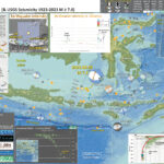
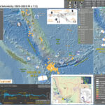
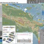
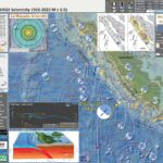
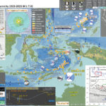
Earthquake Report: M 6.8 Morocco

This evening (my time) there was an earthquake in Morocco. Magnitude 6.8, rather shallow, reverse or thrust (compressional) mechanism.

https://earthquake.usgs.gov/earthquakes/eventpage/us7000kufc/executive

This M 6.8 earthquake happened in the Atlas Mountains, a compressional system with south dipping reverse faults on the north and north dipping reverse faults on the south.

It is possible, if not probable, that this earthquake is related to one of these reverse faults. Based on the location, it seems possible that this earthquake is on a south dipping thrust fault (associated with the North Atlas fault system).

I used the USGS earthquake catalog and it appears that this is the largest magnitude earthquake to happen in Morocco (since we started recording earthquakes on seismometers).

Here is the sobering part of this earthquake. The USGS PAGER Alert provides an estimate for the number of casualties and economic impact. Read more about how these estimates are produced (and how to read this report) here.

UPDATE: (2023.09.10 Version 7)

UPDATE: (2023.09.11)

Fault Scaling Relations

Empirical fault scaling relations are ways that we can compare fault rupture sizes with earthquake magnitudes. One of the most used and well cited empirical fault scaling relations paper is Wells and Coppersmith, 1994.

  • Wells and Coppersmith developed relations between earthquake magnitude/moment magnitude and surface rupture length, subsurface rupture length, and rupture area. They also consider the difference between mean and maximum displacement measures.
  • The length of fault rupture is the distance that the fault slipped measured parallel to Earth’s surface. When we see fault lines mapped on a map, these lines are representative of the fault length.
  • The width of fault rupture is the distance that the fault slipped measured down into the Earth. For a fault that dips straight down into the Earth (perpendicular to the Earth’s surface), the width of the fault rupture is the distance between the Earth’s surface and the depth where the fault slipped. For faults that dip at an angle (like along a subduction zone, or a reverse/thrust fault like the fault that caused this M 6.8 earthquake), the distance measured is measured along this non-perpendicular distance.
  • The area of fault slip is basically the fault length times the fault width.
  • Here is the USGS fault slip model for the M 6.8 earthquake. The length of the fault slip figure is about 40 kilometers (km) and the width of the fault is about 45 km. The color represents the amount that the fault slipped (in meters) during the earthquake. So, the slip area does not fill this entire area. Most of the slip length is within ~30 km and width is within ~35km. The maximum slip is ~1.7 meters.


  • There have been some updates to these scaling relations that attempt to improve these relations. However, Wells and Coppersmith still work pretty well (the updates are not really that much different).
  • There remain certain types of earthquakes where we have small amounts of information to constrain these relations for those types of earthquakes (particularly large magnitude earthquakes, which are more rare than small and medium sized earthquakes). So, there is room for improvement.
  • Here is a plot from Wells and Coppersmith that shows the data relating magnitude with subsurface rupture length. We can see that there is a positive relation between magnitude and length (as the length is larger, so is the magnitude).


    (a) Regression of subsurface rupture length on magnitude (M). Regression line shown for all-slip-type relationship. Short dashed line indicates 95% confidence interval. (b) Regression lines for strike-slip relationships. See
    Table 2 for regression coefficients. Length of regression lines shows the range of data for each relation.

  • Note that there is lots of variation, so these empirical relations (represented by the lines that are drawn to “fit” these data) have lots of range. So, these empirical relations are not perfect predictors (i.e., fault length does not perfectly predict magnitude).
  • For example, a fault with subsurface rupture length of 10 km could have a magnitude that ranges between 5.25 and 6.25+. Remember, a M 6.25 releases about 32 times as much energy as a M 5.25. A M 6.25 earthquake is much larger than a M 5.25.
  • So, I used these scaling relations to calculate the magnitude for earthquakes of varying subsurface fault length. Here is a table from those calculations.


  • The M 6.8 USGS earthquake slip model suggests that this earthquake fits well with these subsurface fault scaling relations from Wells and Coppersmith (1994).
  • Well, as I was wrapping up for the day, I refreshed the USGS website for the earthquake and they had updated a bunch of the data (intensity, GIS data, and the slip data). So, the slip model shows a much smaller slip area. Though, if we look at the EMSC aftershock region, we may think that their first slip model was better. The aftershock region has a better fit for the scaling relations.

Below is my interpretive poster for this earthquake

  • I plot the seismicity from the past month, with diameter representing magnitude (see legend). I include earthquake epicenters from 1922-2022 with magnitudes M ≥ 3.0 in one version.
  • I plot the USGS fault plane solutions (moment tensors in blue and focal mechanisms in orange), possibly in addition to some relevant historic earthquakes.
  • A review of the basic base map variations and data that I use for the interpretive posters can be found on the Earthquake Reports page. I have improved these posters over time and some of this background information applies to the older posters.
  • Some basic fundamentals of earthquake geology and plate tectonics can be found on the Earthquake Plate Tectonic Fundamentals page.

    I include some inset figures. Some of the same figures are located in different places on the larger scale map below.

  • In the upper left corner is a map that shows the tectonic plates and seismicity for northwestern Africa.
  • In the upper right corner is a map that shows the earthquake intensity using the modified Mercalli intensity scale. Earthquake intensity is a measure of how strongly the Earth shakes during an earthquake, so gets smaller the further away one is from the earthquake epicenter. The map colors represent a model of what the intensity may be.
  • Below the intensity map is a plot that shows the same intensity (both modeled and reported) data as displayed on the map. Note how the intensity gets smaller with distance from the earthquake.
  • In the lower left center are two maps showing the probability of earthquake triggered landslides and possibility of earthquake induced liquefaction. I will describe these phenomena below.
  • In the lower right corner is a larger scale map showing the Atlas Mountains and the North and South Atlas faults.
  • To the left of this large scale map is a map from Beauchamp et al., 1999. This map is for the Atlas Mtns to the east of where this earthquake happened. Note the tectonic folds associated with the underlying reverse faults.
  • In the upper left is a map from TEixel et al. (1999) that includes cross section locations. Cross section C is displayed to the right. The location of this cross section is also shown on the main map with the green line.
  • To the left of the intensity map is a map from Banault et al. (2023) that includes a yellow star where the M 6.8 earthquake occurred.
  • Here is the map with a month’s seismicity plotted.

  • This is an updated poster with COMET InSAR analytical results. I also figured out how to download the EMSC seismicity data (they changed their website, so had to learn something new. Here is where one may download data from their catalog.
  • The USGS earthquake catalog (aka ComCat) is a global network, so a global catalog. The EMSC catalog relies, in places, on a more local network, so has more events in the catalog than in ComCat.
  • However, ComCat usually has all the major events and spans a longer time period.
  • SO, the 3 month seismicity I use here is from EMSC and the century dataset is based on the ComCat catalog.

Other Report Pages

Discussion about aftershocks

    the following is a series of statements that i wrote to respond to someone who is in Morocco. i thought that perhaps others might find this useful.

    aftershocks may last for weeks, possibly months. aftershocks typically decay at a rate that is dependent on the fault system. each fault system is slightly different.

    Here is a short story about aftershocks in Northern California but this story is relevant to earthquakes elsewhere.

    we don’t know the specific rate of decay for a fault system until we observe the aftershocks decay for that fault. some faults have few aftershocks and others have robust aftershock sequences (many events).

    it is not satisfying to not know how long they will last, i understand.

    e.g., there was an earthquake in central Washington USA in 1872 and some argue that this continues to have aftershocks.

    so, they will last a while and nobody will know when they will stop.

    but for people to feel safe to start living in their homes again, they need to get an expert, like an engineer, to evaluate the stability of their houses. only an expert, who is trained to inspect structures, can make these evaluations.

    will there be other large earthquakes? this is something nobody can know.

    follow advice for getting an engineer to check out one’s building(s) so that they can feel safe living in them; if the engineer decides that the structure is safe to withstand earthquakes, that is the best we can do.

    the M6.8 changed the stresses in the crust adjacent to the earthquake. in some places, these stresses increased the chance for earthquakes on different (or the same) faults. in other places, they decreased the stress.

    these changes in stress are modest but can trigger a new earthquake. but this depends on the state of stress of the other earthquake fault, something that we cannot yet know. so, we cannot know if the places where stress is increased will have a triggered/new earthquake.

    the best we can do is to make sure that buildings are resistant to earthquake forces. this capability is reliant on engineers, building inspectors, competent building contractors, building codes, etc. AND that these people follow the rules (building codes).

    the Feb 2023 Türkiye earthquakes destroyed buildings that were constructed under well designed building codes. but they were destroyed because people did not follow the code. lots of buildings were built before the codes existed and those did not perform well either.

    so, when living in earthquake country, one simply needs to ensure that they are living/working in earthquake resistant buildings. they may find comfort to live outside these structures until they are inspected. this is the smart thing to do.

    i don’t have the expertise to know if a building is designed to withstand earthquakes. i am not a structural engineer, an earthquake engineer. i know some and can follow the local building codes here where i live. and i sure could not offer advice remotely. one simply needs to seek local expertise. i wish i could offer more advice.

    finally, people who have been traumatized by this earthquake and continue to be traumatized by these aftershocks are going through what everyone does when faced with these conditions. this is typical. maybe finding comfort with friends and family and neighbors will help (?).

    i hope i have provided some constructive feedback to your questions/concerns.

    hopefully this information can help those in Morocco cope with this extremely challenging natural hazard.

    if nothing else, the survivors will be able to build back stronger and more earthquake resistant.

Shaking Intensity

  • Here is a figure that shows a more detailed comparison between the modeled intensity and the reported intensity. Both data use the same color scale, the Modified Mercalli Intensity Scale (MMI). More about this can be found here. The colors and contours on the map are results from the USGS modeled intensity. The DYFI data are plotted as colored dots (color = MMI, diameter = number of reports).
  • In the upper panel is the USGS Did You Feel It reports map, showing reports as colored dots using the MMI color scale. Underlain on this map are colored areas showing the USGS modeled estimate for shaking intensity (MMI scale).
  • In the lower panel is a plot showing MMI intensity (vertical axis) relative to distance from the earthquake (horizontal axis). The models are represented by the green and orange lines. The DYFI data are plotted as light blue dots. The mean and median (different types of “average”) are plotted as orange and purple dots. Note how well the reports fit the green line (the model that represents how MMI works based on quakes in California).
  • Below the lower plot is the USGS MMI Intensity scale, which lists the level of damage for each level of intensity, along with approximate measures of how strongly the ground shakes at these intensities, showing levels in acceleration (Peak Ground Acceleration, PGA) and velocity (Peak Ground Velocity, PGV).

Potential for Ground Failure

Luckily I updated this page because I noticed that the interpretive figure below was incorrect (it was for a different earthquake).

  • Below are a series of maps that show the potential for landslides and liquefaction. These are all USGS data products.
    There are many different ways in which a landslide can be triggered. The first order relations behind slope failure (landslides) is that the “resisting” forces that are preventing slope failure (e.g. the strength of the bedrock or soil) are overcome by the “driving” forces that are pushing this land downwards (e.g. gravity). The ratio of resisting forces to driving forces is called the Factor of Safety (FOS). We can write this ratio like this:

    FOS = Resisting Force / Driving Force

  • When FOS > 1, the slope is stable and when FOS < 1, the slope fails and we get a landslide. The illustration below shows these relations. Note how the slope angle α can take part in this ratio (the steeper the slope, the greater impact of the mass of the slope can contribute to driving forces). The real world is more complicated than the simplified illustration below.

  • Landslide ground shaking can change the Factor of Safety in several ways that might increase the driving force or decrease the resisting force. Keefer (1984) studied a global data set of earthquake triggered landslides and found that larger earthquakes trigger larger and more numerous landslides across a larger area than do smaller earthquakes. Earthquakes can cause landslides because the seismic waves can cause the driving force to increase (the earthquake motions can “push” the land downwards), leading to a landslide. In addition, ground shaking can change the strength of these earth materials (a form of resisting force) with a process called liquefaction.
  • Sediment or soil strength is based upon the ability for sediment particles to push against each other without moving. This is a combination of friction and the forces exerted between these particles. This is loosely what we call the “angle of internal friction.” Liquefaction is a process by which pore pressure increases cause water to push out against the sediment particles so that they are no longer touching.
  • An analogy that some may be familiar with relates to a visit to the beach. When one is walking on the wet sand near the shoreline, the sand may hold the weight of our body generally pretty well. However, if we stop and vibrate our feet back and forth, this causes pore pressure to increase and we sink into the sand as the sand liquefies. Or, at least our feet sink into the sand.
  • Below is a diagram showing how an increase in pore pressure can push against the sediment particles so that they are not touching any more. This allows the particles to move around and this is why our feet sink in the sand in the analogy above. This is also what changes the strength of earth materials such that a landslide can be triggered.

  • Below is a diagram based upon a publication designed to educate the public about landslides and the processes that trigger them (USGS, 2004). Additional background information about landslide types can be found in Highland et al. (2008). There was a variety of landslide types that can be observed surrounding the earthquake region. So, this illustration can help people when they observing the landscape response to the earthquake whether they are using aerial imagery, photos in newspaper or website articles, or videos on social media. Will you be able to locate a landslide scarp or the toe of a landslide? This figure shows a rotational landslide, one where the land rotates along a curvilinear failure surface.

  • Below is the liquefaction susceptibility and landslide probability map (Jessee et al., 2017; Zhu et al., 2017). Please head over to that report for more information about the USGS Ground Failure products (landslides and liquefaction). Basically, earthquakes shake the ground and this ground shaking can cause landslides.
  • I use the same color scheme that the USGS uses on their website. Note how the areas that are more likely to have experienced earthquake induced liquefaction are in the valleys. Learn more about how the USGS prepares these model results here.

Remote Sensing of Surface Deformation

  • One way to learn about the processes that happen during an earthquake is to evaluate the “coseismic” (during earthquake) surface deformation from that earthquake.
  • There are many ways to do this type of analysis. One may use classic surveys (using levels and tape measures) to measure the changes. One may use digital observations from satellites or airplanes, called remote sensing.
  • One of the ways to do this remote sensing is with a method called interferometric synthetic aperture radar (InSAR).
  • The techniques to apply InSAR methods are advanced and take years to master. I will not attempt to explain the full description of what InSAR is but below is a list of online resources where others do a great job at explaining InSAR:
  • Basically, there are satellites that pass over Earth over a regular schedule. These satellites have sensors (called platforms) that acquire a variety of data that span different parts of the electromagnetic spectrum.
  • Many are familiar with the visible light part of the electromagnetic spectrum (recall the Pink Floyd album, The Dark Side of the Moon, which has an image of light going through a prism, showing the different colors of the visible spectrum.
  • The different parts of the electromagnetic spectrum are described by the wavelength of the waves that these different types of radiation use to travel. The wavelength span for blue light is between 400 and 500 nanometers (nm). Green is 500 to 600 nm and red is 600 to 700 nm.
  • Other bands have longer or shorter wavelengths. X-Rays have much shorter wavelengths and infrared radiation has longer wavelengths.
  • Radar operates at long wavelengths (1-100 cm or 10,000,000-1,000,000,000 nm)
  • InSAR analysis, generally, uses radar data collected at two different times to determine how the Earth’s surface moved between the radar acquisitions.
  • There are some organizations that have programs that staff people to work on these InSAR analyses for events like earthquakes. NASA Jet Propulsion Laboratory (JPL) and the Centre for Observation and Modeling of Earthquakes, Volcanoes, and Tectonics (COMET) are two of these programs. They provide the results from their analyses online for anyone to download for free.
  • Here is the COMET event page for this M6.8 Morocco Earthquake.
  • This is a plot of the “unwrapped” InSAR results from the first Sentinel 1 (one of the radar satellites used for InSAR analysis) post-earthquake radar acquisition.
  • Color represents how the surface moved towards or away from the Satellite between 30 August and 11 September 2023. This is an ascending track and once we get a descending track acquisition, we will be able to get a better idea of the coseismic deformation.
  • This result helps us learn that the area in red generally went up and that the fault is dipping to the north (looking at the unwrapped data in the lower panel help with this interpretation).

  • Here is the source of data that I used to plot the above figures.

    Some Relevant Discussion and Figures

    • Here is the tectonic map from the poster (Teizel et al., 2002).

    • (a) Location sketch map of the Atlas Mountains in the North African foreland. (b) Geological map of the central High Atlas, indicating the section lines of Figure 2. ATC, Ait Tamlil basement culmination; SC, Skoura basement culmination; MC, Mougueur basement culmination; FZ, Foum Zabel thrust.

    • Here is the cross section from the poster (Teizel et al., 2002).

    • Serial geological cross sections through the High Atlas of Morocco (location in Figure 1b): (a) Midelt-Errachidia section, (b) Imilchil section, and (c) Demnat section. Segment x–x0 in 2c is adapted from Errarhaoui [1997].

    • This part of the world was once a mid ocean spreading ridge (aka a rifted margin). This figure shows the tectonic plate boundary configurations from this time of Earth’s past.
    • We will revisit this paper further down in the report where we see a geologic map and cross section in the region of this M 6.8 earthquake.

    • Plate reconstruction of the Central Atlantic to the Triassic-Jurassic boundary (200 Ma) (modified from Schettino and Turco, 2009). Rift zones are shown in dark grey. The square indicates the reconstructed position of the Marrakech High Atlas pf Morocco (MHA).

    (Domènech et al., 2015)

    • Here is the Babault et al. (2013) tectonic map.

    • Tectonic sketch map of the Moroccan High Atlas Mountains, indicating the lines of section of Figure 4a, b.

    • Here are the Babault et al. (2013) cross sections.

    • Structural cross-sections across the High Atlas and the Eastern Cordillera of Colombia. (a, b) Sections across the eastern and central High Atlas (from Teixell et al. 2003). These sections are based on field data and were modified from the original according to gravity modelling by Ayarza et al. 2005 (see location in Fig. 1). Although largely eroded, the Cretaceous sediments probably formed a tabular body that covered the entire Atlas domain, representing post-rift conditions. (c) Simplified structural cross-section of the Eastern Cordillera of Colombia, approximately through the latitude of Bogota´ (see location in Fig. 2). This section was constructed on the basis of maps, seismic profiles and structural data provided by ICP-Ecopetrol. The deep structure of the Sabana de Bogota´ region is conjectural as it is poorly imaged in the seismic profiles. The lower–upper Cretaceous boundary is taken for the sake of convenience at the top of the Une and Hilo´ formations. MMVB, Middle Magdalena Valley basin; LLB, Llanos basin.

    • The following are some maps from Lanari et al. (2020).
    • This is the main tectonic map.

    • Location of the study area and simplified geological map of the High Atlas and Anti‐Atlas Mountains. Africa Plate motion considering Eurasia fixed by Serpelloni et al. (2007). FWHA = far western High Atlas; WHA = western High Atlas; CHA = central High Atlas, AA = Anti‐Atlas; MA = Middle Atlas; SAF = South Atlas fault; JTF = Jebilet thrust front.

    • This is a map that shows how complicated the faulting is in this region.

    • Simplified geological map of the study area with schematic logs. See Figure 1 for location. The black lines are the cross‐section traces. Data from Baudon et al. (2009), Domènech et al. (2016, 2015), and El Arabi et al. (2003).

    • Here is a study about the geodetics of the western Mediterranean (Vernant et al., 2010). This study just barely reaches into the western Atlas Mountains, where the M 6.8 earthquake happened.
    • Geodesy is the study of the deformation of the Earth’s surface. Geodesists may study interseismic (between earthquakes) deformation or coseismic (during earthquakes) deformation.
    • These researchers used Global Positioning System (GPS, like in your smartphone) to measure the motion of locations in this area of study.
    • This map shows the two profiles plotted in the next figure. Profile 1 is of interest.

    • (a) GPS site velocities with respect to Nubia and 95% confidence ellipses. Heavy dashed lines show locations of profiles shown in Fig. 3 with the widths of the profiles indicated by lighter dashed lines. Focal mechanism indicates the location of the February 2004 Al Hoceima earthquake. Base map as in Fig. 1. (b) GPS site velocities with respect to Eurasia and 95% confidence ellipses. Format as in (a).

    • Profile 1 makes it into the western Atlas Mountains.
    • On the left, note sites MARO and AZIL. Look at the profile normal plot (the vertical axis represents how much the sites are moving relative to the direction perpendicular to the profile, which is sort of the direction of convergence in the Atlas Mountains).
    • The difference in convergence along the western part of profile 1 shows that there is very little interseismic deformation here. This supports the hypothesis that these faults are low slip rate faults.
    • There does appear to be some amount of interseismic deformation parallel to the profile. This suggests that there is some amount of lateral strain accumulating on these faults. However, these profiles are not oriented in an optimal direction to study the faults in the Atlas Mountains (so my crude interpretations are moderately inaccurate; what do you think about these geodetic data?).

    • Profiles 1 and 2 (see Fig. 2a). (a and d) Component of velocities and 1-sigma uncertainties along the direction of plate motion (normal to profile). (b and e) Component of velocities and 1-sigma uncertainties normal to the direction of plate motion (i.e., parallel to profiles). The interseismic deformation predicted by elastic block models is shown for the three main hypothesized plate boundaries (Red = Klitgord and Schouten, 1986; Green = Bird, 2003; Blue = Gutscher, 2004, see Fig. 1 for geometry). The pink line is for a model with a central Rif block (see the figure for geometry). (c and f) Topography and interpretative cross-section along Profiles 1 and 2. CC = Continental crust, LM= lithospheric mantle, OC= ocean crust, LVA = low velocity, high attenuation seismic anomaly (Calvert et al., 2000a,b).

    UPDATE: 11 Sept 2023

    • Albert Griera tweeted a figure that is included in a reference (Domènech et al., 2015). I used a couple figures from that journal article in an interpretive illustration below.
    • This Domènech et al. (2015) paper includes a cross section very close to the M 6.8 earthquake. At the top of this illustration is the map that shows the geology, faults, and the location for the cross section. Below is this cross section at two different time periods.
    • I include the figure captions for the map and cross section in block quote below the illustration.

    • (a) Geologic map of the western and Marrakech High Atlas (modified from Hollard, 1985), showing location of the study area detailed in (b). (b) Geologic map of the Marrakech High Atlas showing the main structural elements. Squares correspond to areas described in detail in this paper.

      Present-day cross section of the Marrakech High Atlas (see location in Fig. 2) and restoration to a state previous to the orogenic inversion in the Late Cretaceous.

Seismic Hazard and Seismic Risk

  • These are the two maps that show seismic and seismic risk for the western Mediterranean, the GEM Seismic Hazard and the GEM Seismic Risk maps from Pagani et al. (2018) and Silva et al. (2018).
    • The GEM Seismic Hazard Map:


    • The Global Earthquake Model (GEM) Global Seismic Hazard Map (version 2018.1) depicts the geographic distribution of the Peak Ground Acceleration (PGA) with a 10% probability of being exceeded in 50 years, computed for reference rock conditions (shear wave velocity, VS30, of 760-800 m/s). The map was created by collating maps computed using national and regional probabilistic seismic hazard models developed by various institutions and projects, and by GEM Foundation scientists. The OpenQuake engine, an open-source seismic hazard and risk calculation software developed principally by the GEM Foundation, was used to calculate the hazard values. A smoothing methodology was applied to homogenise hazard values along the model borders. The map is based on a database of hazard models described using the OpenQuake engine data format (NRML). Due to possible model limitations, regions portrayed with low hazard may still experience potentially damaging earthquakes.
    • Here is a view of the GEM seismic hazard map for the western Mediterranean.

    • The GEM Seismic Risk Map:


    • The Global Seismic Risk Map (v2018.1) presents the geographic distribution of average annual loss (USD) normalised by the average construction costs of the respective country (USD/m2) due to ground shaking in the residential, commercial and industrial building stock, considering contents, structural and non-structural components. The normalised metric allows a direct comparison of the risk between countries with widely different construction costs. It does not consider the effects of tsunamis, liquefaction, landslides, and fires following earthquakes. The loss estimates are from direct physical damage to buildings due to shaking, and thus damage to infrastructure or indirect losses due to business interruption are not included. The average annual losses are presented on a hexagonal grid, with a spacing of 0.30 x 0.34 decimal degrees (approximately 1,000 km2 at the equator). The average annual losses were computed using the event-based calculator of the OpenQuake engine, an open-source software for seismic hazard and risk analysis developed by the GEM Foundation. The seismic hazard, exposure and vulnerability models employed in these calculations were provided by national institutions, or developed within the scope of regional programs or bilateral collaborations.
    • Here is a view of the GEM seismic risk map for the western Mediterranean.

      References:

      Basic & General References

    • Frisch, W., Meschede, M., Blakey, R., 2011. Plate Tectonics, Springer-Verlag, London, 213 pp.
    • Hayes, G., 2018, Slab2 – A Comprehensive Subduction Zone Geometry Model: U.S. Geological Survey data release, https://doi.org/10.5066/F7PV6JNV.
    • Holt, W. E., C. Kreemer, A. J. Haines, L. Estey, C. Meertens, G. Blewitt, and D. Lavallee (2005), Project helps constrain continental dynamics and seismic hazards, Eos Trans. AGU, 86(41), 383–387, , https://doi.org/10.1029/2005EO410002. /li>
    • Jessee, M.A.N., Hamburger, M. W., Allstadt, K., Wald, D. J., Robeson, S. M., Tanyas, H., et al. (2018). A global empirical model for near-real-time assessment of seismically induced landslides. Journal of Geophysical Research: Earth Surface, 123, 1835–1859. https://doi.org/10.1029/2017JF004494
    • Kreemer, C., J. Haines, W. Holt, G. Blewitt, and D. Lavallee (2000), On the determination of a global strain rate model, Geophys. J. Int., 52(10), 765–770.
    • Kreemer, C., W. E. Holt, and A. J. Haines (2003), An integrated global model of present-day plate motions and plate boundary deformation, Geophys. J. Int., 154(1), 8–34, , https://doi.org/10.1046/j.1365-246X.2003.01917.x.
    • Kreemer, C., G. Blewitt, E.C. Klein, 2014. A geodetic plate motion and Global Strain Rate Model in Geochemistry, Geophysics, Geosystems, v. 15, p. 3849-3889, https://doi.org/10.1002/2014GC005407.
    • Meyer, B., Saltus, R., Chulliat, a., 2017. EMAG2: Earth Magnetic Anomaly Grid (2-arc-minute resolution) Version 3. National Centers for Environmental Information, NOAA. Model. https://doi.org/10.7289/V5H70CVX
    • Müller, R.D., Sdrolias, M., Gaina, C. and Roest, W.R., 2008, Age spreading rates and spreading asymmetry of the world’s ocean crust in Geochemistry, Geophysics, Geosystems, 9, Q04006, https://doi.org/10.1029/2007GC001743
    • Pagani,M. , J. Garcia-Pelaez, R. Gee, K. Johnson, V. Poggi, R. Styron, G. Weatherill, M. Simionato, D. Viganò, L. Danciu, D. Monelli (2018). Global Earthquake Model (GEM) Seismic Hazard Map (version 2018.1 – December 2018), DOI: 10.13117/GEM-GLOBAL-SEISMIC-HAZARD-MAP-2018.1
    • Silva, V ., D Amo-Oduro, A Calderon, J Dabbeek, V Despotaki, L Martins, A Rao, M Simionato, D Viganò, C Yepes, A Acevedo, N Horspool, H Crowley, K Jaiswal, M Journeay, M Pittore, 2018. Global Earthquake Model (GEM) Seismic Risk Map (version 2018.1). https://doi.org/10.13117/GEM-GLOBAL-SEISMIC-RISK-MAP-2018.1
    • Storchak, D. A., D. Di Giacomo, I. Bondár, E. R. Engdahl, J. Harris, W. H. K. Lee, A. Villaseñor, and P. Bormann (2013), Public release of the ISC-GEM global instrumental earthquake catalogue (1900–2009), Seismol. Res. Lett., 84(5), 810–815, doi:10.1785/0220130034.
    • Zhu, J., Baise, L. G., Thompson, E. M., 2017, An Updated Geospatial Liquefaction Model for Global Application, Bulletin of the Seismological Society of America, 107, p 1365-1385, https://doi.org/0.1785/0120160198
    • Specific References

    • Arboleya, M.L., Teoxe;. A., Charroud, M., Julivert, M., 2004. A structural transect through the High and Middle Atlas of Morocco in Journal of African Earth Sciences, v. 39, p. 319-327, https://doi.org/10.1016/j.jafrearsci.2004.07.036
    • Beauchamp, W., Allmendinger, R.W., Barazangi, M., Demnati, A., El Alji, M., and Dahmani, M., 1999. Inversion tectonics and the evolution of the High Atlas Mountains, Morocco, based on a geological-geophysical transect in Tectonics, v. 18, no. 2, p. 163-184, https://doi.org/10.1029/1998TC900015
    • Domènech, M., Teixell, A., Babault, J., and Arbolya, M-L., 2015. The inverted Triassic rift of the Marrakech High Atlas: A reappraisal of basin geometries and faulting histories in Tectonophysics, v. 663, p. 177-191, https://doi.org/10.1016/j.tecto.2015.03.017
    • Domènech, M., Teixell, A., and Stockli, D.F., 2016. Magnitude of rift-related burial and orogenic contraction in the Marrakech High Atlas revealed by zircon(U-Th)/He thermochronology and thermal modeling in Tectonics, v. 35, p. 2609–2635, https://doi.org/10.1002/2016TC004283
    • Jiménez‐Munt, I., M. Fernàndez, J. Vergés, D. Garcia‐Castellanos, J. Fullea, M. Pérez‐Gussinyé, and J. C. Afonso(2011), Decoupled crust‐mantle accommodation of Africa‐Eurasia convergence in the NW Moroccan margin,J. Geophys. Res.,116, B08403, https://doi.org/10.1029/2010JB008105
    • Babault, J., Teixell, A., Struth, L., Van Den Driessche, J., Arboleya, ML., Tesón, and E., 2013. “Shortening, structural relief and drainage evolution in inverted rifts: insights from the Atlas Mountains, the Eastern Cordillera of Colombia and the Pyrenees”, Thick-Skin-Dominated Orogens: From Initial Inversion to Full Accretion, in Nemcˇok, M., Mora, A. & Cosgrove, J. W. (eds) Thick-Skin-Dominated Orogens: From Initial Inversion to Full Accretion. Geological Society, London, Special Publications, 377, http://dx.doi.org/10.1144/SP377.14
    • Lanari, R., Faccenna, C., Fellin, M. G., Essaifi, A., Nahid, A., Medina, F., & Youbi, N. (2020). Tectonic evolution of the western High Atlas of Morocco: Oblique convergence, reactivation, and transpression. Tectonics, 39, e2019TC005563. https://doi.org/10.1029/2019TC005563
    • Teixell, A., Arboleya, M., Julivert, M., and Charroud, M., 2003. Tectonic shortening and topography in the central High Atlas (Morocco) in Tectonics, v. 22, no. 5, 1051, https://doi.org/10.1029/2002TC001460
    • Vernant et al., 2010. Geodetic constraints on active tectonics of the Western Mediterranean: Implications for the kinematics and dynamics of the Nubia-Eurasia plate boundary zone in Journal of Geodynamics, v. 49, no 3-4, p. 123-129, https://doi.org/10.1016/j.jog.2009.10.007

    Return to the Earthquake Reports page.

Earthquake Report: M 7.1 Indonesia

Yesterday on my way home from a Phil & Graham Lesh show, I got a tsunami notification alert from the National Tsunami Warning Center. There was a magnitude M 6.9 earthquake offshore of Indonesia and there was no tsunami threat for the west coast of the US.

I pulled over to investigate and searched the USGS earthquakes page to locate this earthquake. At that time, there were two events spaced closely in time and space. I suspected that there was probably only one earthquake.

Shortly, that turned out to be true (within minutes). There was a M 7.1 earthquake north of the islands of Bali and Lombok, part of Indonesia.

https://earthquake.usgs.gov/earthquakes/eventpage/us7000krjx/executive

There was a series of earthquakes in this area a few years ago, which came to my mind. However, this M 7.1 was much deeper.

This M 7.1 earthquake was quite deep (over 500 km!). Those earlier events were shallower and appear to have been related to the Flores thrust fault. Read more about these shallower earthquakes here.

This part of the world is geologically dominated by the convergent plate margin between the Australia and Eurasia plates. This convergent plate margin is part of the Alpide belt, a convergent plate margin that spans almost half the globe (from the northern tip of Australia to the western tip of Portugal). The Alpide belt is responsible for building the tallest mountains in the world (the Asian Himalayas and the European Alps).

Here, in Indonesia, the Australia plate dives beneath the Australia plate forming a subduction zone and a deep sea trench (the Java trench). Earthquakes along this megathrust subduction zone fault have generated strong ground shaking, generated tsunami, and triggered landslides in the past.

In this part of the world, the Eurasia plate is subdivided into a sub-plate called the Sunda plate (so one might see maps with either name labeling this plate).

As the Australia plate subducts it starts out dipping shallowly beneath Java, Bali, Lombok, and the other islands.

The oceanic crust has water within it that helps generate melt in the magma that exists above the Australia plate and beneath the Sunda plate. When this magma melts, its density decreases and the magma rises until it erupts forming the volcanoes that comprise these islands.

As the Australia plate subducts further, the angle that it dips down into the Earth gets steeper. During this process the plate bends and gets exposed to higher pressures (and temperatures).

These physical processes change the stresses within and surrounding the plate. These changes in stress can cause earthquakes like the M 7.1.

Even though this earthquake was large in magnitude, it was so deep so that the shaking intensity was smaller.

The shaking intensity is often reported using the Modified Mercalli Intensity (MMI) scale. People (anyone with internet access) can report their observations on the USGS “Did You Feel It?” web page for this earthquake.

These observations are then used to estimate the shaking intensity felt by those people. Reports from this earthquake show that people on these nearby islands felt intensities around MMI 4 to MMI 5 or so.

Below is my interpretive poster for this earthquake

  • I plot the seismicity from the past month, with diameter representing magnitude (see legend). I include earthquake epicenters from 1922-2022 with magnitudes M ≥ 3.0 in one version.
  • I plot the USGS fault plane solutions (moment tensors in blue and focal mechanisms in orange), possibly in addition to some relevant historic earthquakes.
  • A review of the basic base map variations and data that I use for the interpretive posters can be found on the Earthquake Reports page. I have improved these posters over time and some of this background information applies to the older posters.
  • Some basic fundamentals of earthquake geology and plate tectonics can be found on the Earthquake Plate Tectonic Fundamentals page.

    I include some inset figures. Some of the same figures are located in different places on the larger scale map below. In some of these inset figures I place a blue star to locate the M 7.1 earthquake on these figures.

  • In the upper right corner is a map showing historic seismicity and tectonic plate boundaries.
  • Below that map is a low angle oblique view of a cut away of the Earth along the subduction zone in Java, Indonesia from EOS.
  • In the upper left corner are maps that show the seismic hazard and seismic risk for Indonesia. I spend more time explaining this below.
  • To the right of these hazard and risk maps is a map that shows earthquake intensity using the Modified Mercalli Intensity (MMI) Scale.
  • Above the map is a plot that shows the same intensity (both modeled and reported) data as displayed on the map. Note how the intensity gets smaller with distance from the earthquake.
  • In the lower right corner is a cross section showing earthquake hypocenters (3-D locations) from Darman et a. (2012).
  • To the left of the Darman (2012) plot is a cross section of seismicity presented by Hengresh and Whitney (2016).
  • In the lower center I plot USGS seismicity from the past century. I describe this further below.
  • Here is the map with a month’s seismicity plotted.

  • Here is the plot with a century’s seismicity plotted.
  • These data are limited to within the region shown on the map and i highlight the M 7.1 in orange.
  • These are USGS hypocenters and epicenters for earthquakes between 1923 and 2023 for magnitudes M≥5.
  • One may observe the seismicity within the Australia plate as the plate subducts downwards. The top of the crust is above these seismicity trends.
  • If one looks closely, they will notice a horizontal line of earthquakes at about 30km. These are all with a default depth of 33 km. There is also a row of seismicity with a default depth of 10km. These are depths assigned to events prior to a location assigned with greater certainty. It is highly likely that the depths for these events is different than 10 or 33 km.

Other Report Pages

    Some Relevant Discussion and Figures

    • Below is a map showing historic seismicity (Jones et al., 2014). Cross sections B-B’ and C-C’ are shown. The seismicity for the cross sections below are sourced from within each respective rectangle.

    • Here are the seismcity cross sections.

    • Here is the map from McCaffrey and Nabelek (1987). They used seismic reflection profiles, gravity modeling along these profiles, seismicity, and earthquake source mechanism analyses to support their interpretations of the structures in this region.

    • Tectonic and geographic map of the eastern Sunda arc and vicinity. Active volcanoes are represented by triangles, and bathymetric contours are in kilometers. Thrust faults are shown with teeth on the upper plate. The dashed box encloses the study area.

    • Here is the Audley (2011) cross section showing how the backthrust relates to the subduction zone beneath Timor. I include their figure caption in blockquote below.

    • Cartoon cross section of Timor today, (cf. Richardson & Blundell 1996, their BIRPS figs 3b, 4b & 7; and their fig. 6 gravity model 2 after Woodside et al. 1989; and Snyder et al. 1996 their fig. 6a). Dimensions of the filled 40 km deep present-day Timor Tectonic Collision Zone are based on BIRPS seismic, earthquake seismicity and gravity data all re-interpreted here from Richardson & Blundell (1996) and from Snyder et al. (1996). NB. The Bobonaro Melange, its broken formation and other facies are not indicated, but they are included with the Gondwana mega-sequence. Note defunct Banda Trench, now the Timor TCZ, filled with Australian continental crust and Asian nappes that occupy all space between Wetar Suture and the 2–3 km deep deformation front north of the axis of the Timor Trough. Note the much younger decollement D5 used exactly the same part of the Jurassic lithology of the Gondwana mega-sequence in the older D1 decollement that produced what appears to be much stronger deformation.

    • This are the seismicity cross sections from Hangesh and Whitney (2016). These are shown to compare the subduction zone offshore of Java and the collision zone in the Timor region.

    • Comparison of hypocentral profiles across the (a) Java subduction zone and (b) Timor collision zone (paleo-Banda trench). Catalog compiled from multiple reporting agencies listed in Table 1. Events of Mw>4.0 are shown for period 1815 to 2015.

    • Below are the maps and cross sections from Darman et al., 2012.
    • Here is the map in the interpretive poster above.

    • Tectonic map of the Lesser Sunda Islands, showing the main tectonic units, main faults, bathymetry and location of seismic sections discussed in this paper.

    • Here is the seismicity cross section in the interpretive poster above.

    • This plot shows the earthquake localizations on a South-North cross section for the lat -14°/-4° long 114°/124° quadrant corresponding to the Lesser Sunda Islands region. The localizations are extracted from the USGS database and corresponds to magnitude greater than 4.5 in the 1973-2004 time period (shallow earthquakes with undetermined depth have been omitted.

    • Here is their interpretations of seismic data used to interpret the tectonics of the subduction zone and Flores thrust.

    • Six 15 km deep seismic sections acquired by BGR from west to east traversing oceanic crust, deep sea trench, accretionary prism, outer arc high and fore-arc basin, derived from Kirchoff prestack depth migration (PreSDM) with a frequency range of 4-60 Hz. Profile BGR06-313 shows exemplarily a velocity-depth model according to refraction/wide-angle
      seismic tomography on coincident profile P31 (modified after Lüschen et al, 2011).

    • Here is a figure showing the regional geodetic motions (Bock et al., 2003). I include their figure caption below as a blockquote.

    • Topographic and tectonic map of the Indonesian archipelago and surrounding region. Labeled, shaded arrows show motion (NUVEL-1A model) of the first-named tectonic plate relative to the second. Solid arrows are velocity vectors derived from GPS surveys from 1991 through 2001, in ITRF2000. For clarity, only a few of the vectors for Sumatra are included. The detailed velocity field for Sumatra is shown in Figure 5. Velocity vector ellipses indicate 2-D 95% confidence levels based on the formal (white noise only) uncertainty estimates. NGT, New Guinea Trench; NST, North Sulawesi Trench; SF, Sumatran Fault; TAF, Tarera-Aiduna Fault. Bathymetry [Smith and Sandwell, 1997] in this and all subsequent figures contoured at 2 km intervals.

    • In addition to the orientation of relative plate motion (that controls seismogenic zone and strain partitioning), the Indo Australia plate varies in crustal age (Lasitha et al., 2006). I include their figure caption below as a blockquote.

    • Tectonic sketch map of the Sumatra–Java trench-arc region in eastern Indian Ocean Benioff Zone configuration. Hatched line with numbers indicates depth to the top of the Benioff Zone (after Newcomb and McCann13). Magnetic anomaly identifications have been considered from Liu et al.14 and Krishna et al.15. Magnitude and direction of the plate motion is obtained from Sieh and Natawidjaja11. O indicates the location of the recent major earthquakes of 26 December 2004, i.e. the devastating tsunamigenic earthquake (Mw = 9.3) and the 28 March 2005 earthquake (Mw = 8.6).

    • Below are the 4 figures from Koulani et al., 2016. First is the plate tectonic map. I include their figure captions in block quote.

    • Seismotectonic setting of the Sunda-Banda arc-continent collision, East Indonesia. Major faults (thick black lines) [Hamilton, 1979]. Topography and bathymetry are from Shuttle Radar Topography Mission (http://topex.ucsd.edu/www_html/srtm30_plus.html). Focal mechanisms are from the Global Centroid Moment Tensor. Blue mechanisms correspond to earthquakes with Mw>7 (brown transparent ellipses are the corresponding rupture areas for Flores 1992 and Alor 2004 earthquakes), while the green focal mechanism shows the highest magnitude recorded in Sumbawa. Red dots indicate the locations of major historical earthquakes [Musson, 2012].

    • This figure shows their estimates for plate motion relative velocities as derived from GPS data, constrained by the fault geometry in their block modeling.

    • GPS velocities determined in this study with respect to Sunda Block. Uncertainty ellipses represent 95% confidence level. The inset figure corresponds to the area of the dashed rectangle in the map. Light blue arrows show the velocities for East and West Makassar Blocks.

    • This figure shows their estimates of slip rate deficit along all the plate boundary faults in this region.

    • Relative slip vectors across block boundaries, derived from our best fit model. Arrows show motion of the hanging wall (moving block) relative to the footwall (fixed block) with 95% confidence ellipses. The tails of arrows is located within the “moving” block. Black thick lines show well-defined boundaries we use as active faults in our model and dashed lines show less well-defined boundaries (green : free-slipping boundaries and black: fixed locked faults) . Principal axes of the horizontal strain tensor estimated for the SUMB, EMAK, and EJAV are shown in pink. The thick pink arrow shows the relative motion of Australia with respect to Sunda (AUST/SUND). Abbreviations are Sumba Block (SUMB), West Makassar Block (WMAK), East Makassar Block (EMAK), East Java Block (EJAV), and Timor Block (TIMO). The background seismicity is from the International Seismological Centre catalog with magnitudes ≥5.5 and depths <40 km.

    • Here is their figure that shows the slip deficit along the plate boundary faults.

    • Fault slip rate components: (a) fault normal (extension positive) and (b) fault parallel (right-lateral positive).

    Seismic Hazard and Seismic Risk

    • These are the two maps shown in the map above, the GEM Seismic Hazard and the GEM Seismic Risk maps from Pagani et al. (2018) and Silva et al. (2018).
      • The GEM Seismic Hazard Map:


      • The Global Earthquake Model (GEM) Global Seismic Hazard Map (version 2018.1) depicts the geographic distribution of the Peak Ground Acceleration (PGA) with a 10% probability of being exceeded in 50 years, computed for reference rock conditions (shear wave velocity, VS30, of 760-800 m/s). The map was created by collating maps computed using national and regional probabilistic seismic hazard models developed by various institutions and projects, and by GEM Foundation scientists. The OpenQuake engine, an open-source seismic hazard and risk calculation software developed principally by the GEM Foundation, was used to calculate the hazard values. A smoothing methodology was applied to homogenise hazard values along the model borders. The map is based on a database of hazard models described using the OpenQuake engine data format (NRML). Due to possible model limitations, regions portrayed with low hazard may still experience potentially damaging earthquakes.
      • Here is a view of the GEM seismic hazard map for Indonesia.

      • The GEM Seismic Risk Map:


      • The Global Seismic Risk Map (v2018.1) presents the geographic distribution of average annual loss (USD) normalised by the average construction costs of the respective country (USD/m2) due to ground shaking in the residential, commercial and industrial building stock, considering contents, structural and non-structural components. The normalised metric allows a direct comparison of the risk between countries with widely different construction costs. It does not consider the effects of tsunamis, liquefaction, landslides, and fires following earthquakes. The loss estimates are from direct physical damage to buildings due to shaking, and thus damage to infrastructure or indirect losses due to business interruption are not included. The average annual losses are presented on a hexagonal grid, with a spacing of 0.30 x 0.34 decimal degrees (approximately 1,000 km2 at the equator). The average annual losses were computed using the event-based calculator of the OpenQuake engine, an open-source software for seismic hazard and risk analysis developed by the GEM Foundation. The seismic hazard, exposure and vulnerability models employed in these calculations were provided by national institutions, or developed within the scope of regional programs or bilateral collaborations.
    • Here is a view of the GEM seismic risk map for Indonesia.

    Tsunami Hazard

    • Here are two maps that show the results of probabilistic tsunami modeling for the nation of Indonesia (Horspool et al., 2014). These results are similar to results from seismic hazards analysis and maps. The color represents the chance that a given area will experience a certain size tsunami (or larger).
    • The first map shows the annual chance of a tsunami with a height of at least 0.5 m (1.5 feet). The second map shows the chance that there will be a tsunami at least 3 meters (10 feet) high at the coast.

    • Annual probability of experiencing a tsunami with a height at the coast of (a) 0.5m (a tsunami warning) and (b) 3m (a major tsunami warning).

    References:

    Basic & General References

  • Frisch, W., Meschede, M., Blakey, R., 2011. Plate Tectonics, Springer-Verlag, London, 213 pp.
  • Hayes, G., 2018, Slab2 – A Comprehensive Subduction Zone Geometry Model: U.S. Geological Survey data release, https://doi.org/10.5066/F7PV6JNV.
  • Holt, W. E., C. Kreemer, A. J. Haines, L. Estey, C. Meertens, G. Blewitt, and D. Lavallee (2005), Project helps constrain continental dynamics and seismic hazards, Eos Trans. AGU, 86(41), 383–387, , https://doi.org/10.1029/2005EO410002. /li>
  • Jessee, M.A.N., Hamburger, M. W., Allstadt, K., Wald, D. J., Robeson, S. M., Tanyas, H., et al. (2018). A global empirical model for near-real-time assessment of seismically induced landslides. Journal of Geophysical Research: Earth Surface, 123, 1835–1859. https://doi.org/10.1029/2017JF004494
  • Kreemer, C., J. Haines, W. Holt, G. Blewitt, and D. Lavallee (2000), On the determination of a global strain rate model, Geophys. J. Int., 52(10), 765–770.
  • Kreemer, C., W. E. Holt, and A. J. Haines (2003), An integrated global model of present-day plate motions and plate boundary deformation, Geophys. J. Int., 154(1), 8–34, , https://doi.org/10.1046/j.1365-246X.2003.01917.x.
  • Kreemer, C., G. Blewitt, E.C. Klein, 2014. A geodetic plate motion and Global Strain Rate Model in Geochemistry, Geophysics, Geosystems, v. 15, p. 3849-3889, https://doi.org/10.1002/2014GC005407.
  • Meyer, B., Saltus, R., Chulliat, a., 2017. EMAG2: Earth Magnetic Anomaly Grid (2-arc-minute resolution) Version 3. National Centers for Environmental Information, NOAA. Model. https://doi.org/10.7289/V5H70CVX
  • Müller, R.D., Sdrolias, M., Gaina, C. and Roest, W.R., 2008, Age spreading rates and spreading asymmetry of the world’s ocean crust in Geochemistry, Geophysics, Geosystems, 9, Q04006, https://doi.org/10.1029/2007GC001743
  • Pagani,M. , J. Garcia-Pelaez, R. Gee, K. Johnson, V. Poggi, R. Styron, G. Weatherill, M. Simionato, D. Viganò, L. Danciu, D. Monelli (2018). Global Earthquake Model (GEM) Seismic Hazard Map (version 2018.1 – December 2018), DOI: 10.13117/GEM-GLOBAL-SEISMIC-HAZARD-MAP-2018.1
  • Silva, V ., D Amo-Oduro, A Calderon, J Dabbeek, V Despotaki, L Martins, A Rao, M Simionato, D Viganò, C Yepes, A Acevedo, N Horspool, H Crowley, K Jaiswal, M Journeay, M Pittore, 2018. Global Earthquake Model (GEM) Seismic Risk Map (version 2018.1). https://doi.org/10.13117/GEM-GLOBAL-SEISMIC-RISK-MAP-2018.1
  • Storchak, D. A., D. Di Giacomo, I. Bondár, E. R. Engdahl, J. Harris, W. H. K. Lee, A. Villaseñor, and P. Bormann (2013), Public release of the ISC-GEM global instrumental earthquake catalogue (1900–2009), Seismol. Res. Lett., 84(5), 810–815, doi:10.1785/0220130034.
  • Zhu, J., Baise, L. G., Thompson, E. M., 2017, An Updated Geospatial Liquefaction Model for Global Application, Bulletin of the Seismological Society of America, 107, p 1365-1385, https://doi.org/0.1785/0120160198
  • Specific References

  • Audley-Charles, M.G., 1986. Rates of Neogene and Quaternary tectonic movements in the Southern Banda Arc based on micropalaeontology in: Journal of the Geological Society, London, Vol. 143, 1986, pp. 161-175.
  • Audley-Charles, M.G., 2011. Tectonic post-collision processes in Timor, Hall, R., Cottam, M. A. &Wilson, M. E. J. (eds) The SE Asian Gateway: History and Tectonics of the Australia–Asia Collision. Geological Society, London, Special Publications, 355, 241–266.
  • Baldwin, S.L., Fitzgerald, P.G., and Webb, L.E., 2012. Tectonics of the New Guinea Region in Annu. Rev. Earth Planet. Sci., v. 41, p. 485-520.
  • Benz, H.M., Herman, Matthew, Tarr, A.C., Hayes, G.P., Furlong, K.P., Villaseñor, Antonio, Dart, R.L., and Rhea, Susan, 2011. Seismicity of the Earth 1900–2010 New Guinea and vicinity: U.S. Geological Survey Open-File Report 2010–1083-H, scale 1:8,000,000.
  • Darman, H., 2012. Seismic Expression of Tectonic Features in the Lesser Sunda Islands, Indonesia in Berita Sedimentologi, Indonesian Journal of Sedimentary Geology, no. 25, po. 16-25.
  • Hall, R., 2011. Australia-SE Asia collision: plate tectonics and crustal flow in Geological Society, London, Special Publications 2011; v. 355; p. 75-109 doi: 10.1144/SP355.5
  • Hangesh, J. and Whitney, B., 2014. Quaternary Reactivation of Australia’s Western Passive Margin: Inception of a New Plate Boundary? in: 5th International INQUA Meeting on Paleoseismology, Active Tectonics and Archeoseismology (PATA), 21-27 September 2014, Busan, Korea, 4 pp.
  • Hayes, G.P., Wald, D.J., and Johnson, R.L., 2012. Slab1.0: A three-dimensional model of global subduction zone geometries in, J. Geophys. Res., 117, B01302, doi:10.1029/2011JB008524
  • Jones, E.S., Hayes, G.P., Bernardino, Melissa, Dannemann, F.K., Furlong, K.P., Benz, H.M., and Villaseñor, Antonio, 2014. Seismicity of the Earth 1900–2012 Java and vicinity: U.S. Geological Survey Open-File Report 2010–1083-N, 1 sheet, scale 1:5,000,000, https://dx.doi.org/10.3133/ofr20101083N.
  • Koulali, A., S. Susilo, S. McClusky, I. Meilano, P. Cummins, P. Tregoning, G. Lister, J. Efendi, and M. A. Syafi’i, 2016. Crustal strain partitioning and the associated earthquake hazard in the eastern Sunda-Banda Arc in Geophys. Res. Lett., 43, 1943–1949, doi:10.1002/2016GL067941
  • Krabbenhoeft, A., Weinrebe, R.W., Kopp, H., Flueh, E.R., Ladage, S., Papenberg, C., Planert, L., and Djajadihardja, Y., 2010. Bathymetry of the Indonesian Sunda margin-relating morphological features of the upper plate slopes to the location and extent of the seismogenic zone in NHESS, v. 10, p. 1899-1911, doi:10.5194/nhess-10-1899-2010
  • McCaffrey, R., and Nabelek, J.L., 1984. The geometry of back arc thrusting along the Eastern Sunda Arc, Indonesia: Constraints from earthquake and gravity data in JGR, Atm., vol., 925, no. B1, p. 441-4620, DOI: 10.1029/JB089iB07p06171
  • Okal, E. A., & Reymond, D., 2003. The mechanism of great Banda Sea earthquake of 1 February 1938: applying the method of preliminary determination of focal mechanism to a historical event in EPSL, v. 216, p. 1-15.
  • Silver, E.A., Breen, N.A., and Prastyo, H., 1986. Multibeam Study of the Flores Backarc Thrust Belt, Indonesia, in JGR., vol. 91, no. B3, p. 3489-3500
  • Zahirovic, S., Seton, M., and Müller, R.D., 2014. The Cretaceous and Cenozoic tectonic evolution of Southeast Asia in Solid Earth, v. 5, p. 227-273, doi:10.5194/se-5-227-2014

Return to the Earthquake Reports page.

Earthquake Report: M 7.7 Loyalty Islands

I am catching up with this today as I have been busy with other things.

I am still behind on those things, but wanted to get this put together since I am currently working on a project that includes tsunami sources in this region.

There was a magnitude M 7.7 earthquake on 19 May 2023 offshore of New Caledonia.

https://earthquake.usgs.gov/earthquakes/eventpage/at00ruvxj7/executive

This earthquake happened in the Australia plate, west of the deep sea trench.

The deep sea trench owes its existence to the plate boundary fault system there, a convergent plate boundary where plates move towards each other. The plate boundary here is formed by the subduction of the Australia plate beneath the North Fiji Basin.

The largest earthquakes that happen on Earth happen on these subduction zone faults.

At first I thought that this was an interface earthquake along the megathrust subduction zone fault. These are called interface events because they happen along the fault interface between the two plates. They are also called interplate earthquakes.

However, the location showed this to be west of the subduction zone. Also, as the earthquake mechanisms (e.g., focal mechanism or moment tensor) were calculated and posted online, it was clear that this was not a megathrust earthquake.

Here is an illustration that shows a cross section of a subduction zone. I show hypothetical locations for different types of earthquakes. I include earthquake mechanisms (as they would be viewed from map view) for these different types of earthquakes.


Here is a legend for these different mechanisms. We can see what the mechanisms look like from map view (from looking down onto Earth from outer space or from flying in an airplane) and what they look like from the side.


The mechanism for the M 7.7 Loyalty Isles earthquake is an extensional (normal) type of an earthquake that happened in the slab of the Australia plate.

Typically, the extension in these slab events is perpendicular to the plate boundary fault because that is the direction that the plate is pulling down (slab pull) due to gravity or that is the orientation of bending of the plate that causes this extension.

There are also records of tsunami and seismic waves on water level sensors in this region. A tsunami was observed on the Ouinne (New Caledonia) tide gage.

Here are the tide gage data from https://webcritech.jrc.ec.europa.eu/SeaLevelsDb/Home.

This M 7.7 earthquake is having lots of aftershocks and the largest was a M 7.1.

https://earthquake.usgs.gov/earthquakes/eventpage/us6000kdce/executive

Not only did the M 7.7 generate a tsunami but so did the M 7.1 earthquake. The plot below shows both earthquake times relative to the tsunami produced by those events.

These tsunami were recorded on other gages as well but this was the best record I saw.


My initial tweet called this normal faulting event a tensional earthquake. Dr. Harold Tobin provided an excellent overview of the difference between tension and extension.

Below is my interpretive poster for this earthquake

  • I plot the seismicity from the past month, with diameter representing magnitude (see legend). I include earthquake epicenters from 1923-2023 with magnitudes M ≥ 7.5 in one version.
  • I plot the USGS fault plane solutions (moment tensors in blue and focal mechanisms in orange), possibly in addition to some relevant historic earthquakes.
  • A review of the basic base map variations and data that I use for the interpretive posters can be found on the Earthquake Reports page. I have improved these posters over time and some of this background information applies to the older posters.
  • Some basic fundamentals of earthquake geology and plate tectonics can be found on the Earthquake Plate Tectonic Fundamentals page.

    I include some inset figures. Some of the same figures are located in different places on the larger scale map below.

  • In the lower center is a tectonic map from Patriat et al. (2019). I place a yellow star in the general location of this M 7.7 earthquake.
  • In the upper left corner shows the tectonic plates and seismicity from the past century for events with magnitudes larger than M 7.5.
  • Below this map is a figure from the USGS that shows their estimate of how much the fault slipped during this M 7.7 earthquake. Dark red shows where the fault may have slipped as much as 3 meters.
  • In the lower right corner is a map that shows the earthquake intensity using the modified Mercalli intensity scale. Earthquake intensity is a measure of how strongly the Earth shakes during an earthquake, so gets smaller the further away one is from the earthquake epicenter. The map colors represent a model of what the intensity may be. The USGS has a system called “Did You Feel It?” (DYFI) where people enter their observations from the earthquake and the USGS calculates what the intensity was for that person. The transparent colors with yellow labels show what people actually felt in those different locations.
  • in the lower left is the tide gage plot from Ouinne, New Caledonia (location shown on the map).
  • In the upper right is a map that shows earthquakes and their aftershock sequences for three events in the past 3 years. There is some overlap, but mostly, these three sequences have aftershocks in different areas. The 2021 and 2022 earthquakes are probably (?) subduction zone earthquakes based on their mechanisms. it sure seems like these two events may have changed the stresses in the Australia plate (i.e., they may have triggered the 2023 earthquake).
    1. 2021 M 7.7 (green)
    2. 2022 M 7.0 (blue)
    3. 2023 M 7.7 (orange)
  • Here is the map with a month’s seismicity plotted.

    Other Report Pages

    Some Relevant Discussion and Figures

    The U.S. Geological Survey (USGS) has a spectacular web page that helps us learn about the plate tectonics (seismotectonics) of the eastern margin of the Australia plate. Check out their webpage here.

    • Here is the plate tectonic map from Patriat et al. (2019).

    • A) Simplified present-day geodynamic map of the New Hebrides and Matthew-Hunter subduction systems (modern trenches shown in black). Inferred location of the New Hebrides subduction and its termination as a STEP fault before 2 Ma shown in light grey. Inset map shows the regional bathymetry. B) Schematic evolution of the North Fiji Basin when the system shifted from a STEP fault to subduction initiation at 2 Ma (after Patriat et al., 2015). LR, Loyalty Ridge; NC, New Caledonia.

    • This is the plate tectonic map from de Alteriis et al. (1993) that shows the major fault systems in the region.

    • Location map of North Fiji Basin ridge; box indicates full multibeam covered area of Figure 2. Heavy lines denote north-south, N15°, and N160° main segments of ridge axis; dashed lines are pseudofaults indicating double propagation. F. Z.— fracture zone.

    • Here is a figure from Schellart et al. (2002) that shows their model of tectonic development of the North Fiji Basin. Schellart et al. (2002) include a long list of references for the tectonics in this region here. Below I include the text from the original figure caption in blockquote.

    • Tectonic reconstruction of the New Hebrides – Tonga region (modified and interpreted from Auzende et al. [1988], Pelletier et al. [1993], Hathway [1993] and Schellart et al.(2002a)) at (a) ~ 13 Ma, (b) ~ 9 Ma, (c) 5 Ma and (d) Present. The Indo-Australian plate is fixed. DER = d’Entrcasteaux Ridge, HFZ = Hunter Fracture Zone, NHT = New Hebrides Trench, TT = Tonga Trench, WTP = West Torres Plateau. Arrows indicate direction of arc migration. During opening of the North Fiji Basin, the New Hebrides block has rotated some 40-50° clockwise [Musgrave and Firth 1999], while the Fiji Plateau has rotated some 70-115° anticlockwise [Malahoff et al. 1982]. During opening of the Lau Basin, the Tonga Ridge has rotated ~ 20° clockwise [Sager et al. 1994]. (Click for enlargement)

    • This is the plate tectonic history map from Begg and Gray (1993) that shows how they interpret the Fiji Plateau to have formed.

    • Tectonic setting (Figures 1a–1c) and tectonic reconstructions (Figures 1d and 1e) of the Outer Melanesian region (adapted from Hathway [1993]; reprinted with permission from the Geological Society of London).

    • (a) Map of the Fiji platform and north end of the Lau Ridge showing the major islands in the Fiji area, the major early Pliocene volcanoes of Viti Levu, the major seafloor fracture zones, and part of the spreading center of the Fiji Basin (adapted from Gill and Whelan [1989]). Shoshonitic volcanoes, including the Tavua Volcano (T), are shown by squares and calc-alkaline volcanoes by circles.
    • (b) Tectonic features of the northeastern segment of the plate boundary between the Australian and Pacific plates showing the Outer Melanesian Arc of the southwest Pacific, trenches and ridge systems, and oceanic plateaus (adapted from Kroenke [1984]). Fiji, as part of the Fiji Platform, consists of a series of islands at the north end of the Lau Ridge, with the North Fiji Basin formed as part of a spreading center.
    • (c) Present plate configuration.
    • (d) Reconstruction at 5.5 Ma.
    • (e) Reconstruction at 10 Ma. In Figures 1a–1e the Australian plate is fixed and the east-west convergence rate between plates was assumed to be 9–10 cm yr-1. Shading represents submarine depths <2000 m.
    • Abbreviations are as follows: VT, Vitiaz trench; VAT, Vanuatu trench; LR, Lau Ridge; LB, Lau Basin; TR, Tonga Ridge; FFZ, Fiji Fracture Zone; LL, Lomaiviti lineament; V-BL, Vatulele-Beqa lineament. Long dashes denote southern margin of the Melanesian Border Plateau (MBP). The open square (Figures 1b and 1c) denotes the location of the Tavua Volcano.
    • Here are figures from Richards et al. (2011) with their figure captions below in blockquote.
    • The main tectonic map

    • bathymetry, and major tectonic element map of the study area. The Tonga and Vanuatu subduction systems are shown together with the locations of earthquake epicenters discussed herein. Earthquakes between 0 and 70 km depth have been removed for clarity. Remaining earthquakes are color-coded according to depth. Earthquakes located at 500–650 km depth beneath the North Fiji Basin are also shown. Plate motions for Vanuatu are from the U.S. Geological Survey, and for Tonga from Beavan et al. (2002) (see text for details). Dashed line indicates location of cross section shown in Figure 3. NFB—North Fiji Basin; HFZ—Hunter Fracture Zone.

    • Here is the map showing the current configuration of the slabs in the region.

    • Map showing distribution of slab segments beneath the Tonga-Vanuatu region. West-dipping Pacifi c slab is shown in gray; northeast-dipping Australian slab is shown in red. Three detached segments of Australian slab lie below the North Fiji Basin (NFB). HFZ—Hunter Fracture Zone. Contour interval is 100 km. Detached segments of Australian plate form sub-horizontal sheets located at ~600 km depth. White dashed line shows outline of the subducted slab fragments when reconstructed from 660 km depth to the surface. When all subducted components are brought to the surface, the geometry closely approximates that of the North Fiji Basin.

    • This is the cross section showing the megathrust fault configuration based on seismic tomography and seismicity.

    • Previous interpretation of combined P-wave tomography and seismicity from van der Hilst (1995). Earthquake hypocenters are shown in blue. The previous interpretation of slab structure is contained within the black dashed lines. Solid red lines mark the surface of the Pacifi c slab (1), the still attached subducting Australian slab (2a), and the detached segment of the Australian plate (2b). UM—upper mantle;
      TZ—transition zone; LM—lower mantle.

    • Here is their time step interpretation of the slabs that resulted in the second figure above.

    • Simplified plate tectonic reconstruction showing the progressive geometric evolution of the Vanuatu and Tonga subduction systems in plan view and in cross section. Initiation of the Vanuatu subduction system begins by 10 Ma. Initial detachment of the basal part of the Australian slab begins at ca. 5–4 Ma and then sinking and collision between the detached segment and the Pacifi c slab occur by 3–4 Ma. Initial opening of the Lau backarc also occurred at this time. Between 3 Ma and the present, both slabs have been sinking progressively to their current position. VT—Vitiaz trench; dER—d’Entrecasteaux Ridge.

    • Here is a map from the USGS report (Benz et al., 2011). Read more about this map on the USGS website. Earthquakes are plotted with color related to depth and circle diameter related to magnitude. Today’s M 6.8 earthquake occurred south of cross section G-G’.

    • This is the legend.

    • Here is a cross section showing the seismicity along swatch profile G-G’.


    • Craig et al. (2014) evaluated the historic record of seismicity for subduction zones globally. In particular, the evaluated the relations between upper and lower plate stresses and earthquake types (cogent for the southern New Hebrides trench). Below is a figure from their paper for this part of the world. I include their figure caption below in blockquote.

    • Outer-rise seismicity along the New Hebrides arc. (a) Seismicity and focal mechanisms. Seismicity at the southern end of the arc is dominated by two major outer-rise normal faulting events, and MW 7.6 on 1995 May 16 and an MW 7.1 on 2004 January 3. Earthquakes are included from Chapple & Forsyth (1979); Chinn & Isacks (1983); Liu & McNally (1993). (b) Time versus latitude plot.

    • Here is a summary figure from Craig et al. (2014) that shows different stress configurations possibly existing along subduction zones.

    • Schematic diagram for the factors influencing the depth of the transition from horizontal extension to horizontal compression beneath the outer rise. Slab pull, the interaction of the descending slab with the 660 km discontinuity (or increasing drag from the surround mantle), and variations in the interface stress influence both the bending moment and the in-plane stress. Increases in the angle of slab dip increases the dominance of the bending moment relative to the in-plane stress, and hence moves the depth of transition towards the middle of the mechanical plate from either an shallower or a deeper position. A decrease in slab dip enhances the influence of the in-plane stress, and hence moves the transition further from the middle of the mechanical plate, either deeper for an extensional in-plane stress, or shallower for a compressional in-plane stress. Increased plate age of the incoming plate leads to increases in the magnitude of ridge push and intraplate thermal contraction, increasing the in-plane compressional stress in the plate prior to bending. Dynamic topography of the oceanic plate seawards of the trench can result in either in-plane extension or compression prior to the application of the bending stresses.

    • Here is an animation that shows the seismicity for this region from 1960 – 2016 for earthquakes with magnitudes greater than or equal to 7.0.
    • I include some figures mentioned in my report from 2016.04.28 for a sequence of earthquakes in the same region as today’s earthquake (albeit shallower hypocentral depths), in addition to a plot from Cleveland et al. (2014). In the upper right corner, Cleveland et al. (2014) on the left plot a map showing earthquake epicenters for the time period listed below the plot on the right. On the right is a plot of earthquakes (diameter = magnitude) of earthquakes with latitude on the vertical axis and time on the horizontal axis. Cleveland et al (2014) discuss these short periods of seismicity that span a certain range of fault length along the New Hebrides Trench in this area. Above is a screen shot image and below is the video. To see more about the tectonics in the Vanuatu region, head over to a report from January 2023.

    • Here is a link to the embedded video below (6 MB mp4)
    • Here is a great overview map from Schellart et al. (2006).
    • There is a cross section in subsequent figures and the location of this section is shown on the map on the left.

    • (a) Topography and bathymetry of the Southwest Pacific region (from Smith and Sandwell (1997)) and (b) regional tectonic setting of (a). Cfz, Cook fracture zone; ChRfsz, Chatham Rise fossil subduction zone; d’ER, d’Entrecasteaux Ridge; EP, East Papua; ER, Efate Re-entrant; LPl, Louisiade Plateau; LoR, Loyalty Ridge; LTr, Louisiade Trough; MaB, Manus Basin; MeR, Melish Rise; NB, New Britain; NBT, New Britain Trench; NCfsz, New Caledonia fossil subduction zone; Nd’EB, North d’Entrecasteaux Basin; NHT, New Hebrides Trench; NLoB, North Loyalty Basin; NST, North Solomon Trough; QT, Queensland Trough; ReB, Reinga Basin, ReR, Reinga Ridge; SCB, Santa Cruz Basin; SCT, San Cristobal Trench; SER, South Efate Re-entrant; SLoB, South Loyalty Basin; SoS, Solomon Sea; SReT, South Rennell Trough; TaB, Taranaki Basin; TKR, Three Kings Ridge; ToT, Townsville Trough; TrT, Trobriand Trough; VMfz, Vening Meinesz fracture zone;WoB,Woodlark Basin; WTP,West Torres Plateau. 1, normal fault; 2, strike-slip fault; 3, subduction zone; 4, spreading ridge (double line) and transform faults (single lines); 5, land; 6–8, sea, with 6, continental or arc crust; 7, oceanic plateau; and 8, basin/ocean floor. Structures in light grey indicate that they are inactive. Thick continuous east–west line at latitude 20° S in panel (a) shows location of cross-section plotted in Fig. 4h. Thick dashed line in panel (a) shows location of cross-section plotted in Fig. 5.

    • Below is a series of cross sections (location on above map) through time.
    • The panels start at 85 million years ago (Ma) and proceed to the present time (panel H).


    • East–west cross-sections illustrating the evolution of the Southwest Pacific region since the Cretaceous in an Australia-fixed reference frame. For location of final cross-section in Fig. 4h see Fig. 1. White arrows indicate convergence between Pacific plate and Australia. Black arrows illustrate the sinking kinematics of a slab. Diagrams illustrate that subduction of Pacific lithosphere from the Late Cretaceous to Paleocene and subduction of backarc lithosphere (e.g. South Loyalty slab) results primarily from slab rollback (i.e. negligible convergence between overriding and subducting plate), leading to a simple slab geometry with draping of the slab over the upper–lower mantle discontinuity. subduction of the Pacific plate from the Eocene to Present results from both slab rollback and convergence, leading to a more complex slab geometry with slab draping (due to rollback) and folding (due to convergence). Slab kinematics was inspired by subduction models from Guillou-Frottier et al. (1995), Griffiths et al. (1995), Funiciello et al. (2003) and Schellart (2004a, 2005).

    • Here is a reconstruction that Schellart et al. (2006) prepared for the past 10 Ma.

    • Reconstruction of the clockwise rotation of the New Hebrides arc during opening of the North Fiji backarc Basin, resulting in collision of the arc with the d’Entrecasteaux Ridge and formation of the Efate re-entrant during initial collision. Location of the initial collision site provides an estimate of the eastward continuation of the d’Entrecasteaux Ridge, and therefore an estimate of the east–west width of the South Loyalty Basin (∼750km). Location of the rotation pole is indicated by the black dot and the curved arrow. Numbers indicate approximate amount of rotation of the New Hebrides arc since opening of the North Fiji Basin at ∼12–11Ma. Australia is fixed. Hfz, Hunter fracture zone; LB, Lau Basin; NFB, North Fiji Basin; NHT, New Hebrides Trench; SCT, San Cristobal Trench.

    • Here is an interesting paper where van de Lagemaat et al. (2018) work out the tectonic history of the region between New Zealand, Australia, and the Loyalty Islands.
    • They prepare a tectonic model to reconstruct the tectonic history and compare their model with seismic tomography models.

    • Topography and bathymetry (left) and tectonic map (right) of the SW Pacific. Tectonic map is based on our model (see Table 3 and the supporting information): continents in green, submerged continental fragments and volcanic arcs in gray. Present-day plate boundaries in red, former plate boundaries in dark gray. Pink and yellow stars are locations of New Caledonia and Northland ophiolites, respectively. (Former) plate names in dark blue. SW Pacific assemblage consists of multiple smaller plates. BT = Bellona Trough; DEB = D’Entrecasteaux Basin; DEZ = D’Entrecasteaux Zone; FAB = Fairway- Aotea Basin; HT = Havre Trough; KAP = Kupe Abyssal Plain; MAP = Minerva Abyssal Plain = NB, Norfolk Basin; NCB = New Caledonia Basin; NFB = North Fiji Basin; NLB = North Loyalty Basin; LB = Lau Basin; SFB = South Fiji Basin; SLB = South Loyalty Basin; WB = Woodlark Basin; NHT = New Hebdrides Trench; Cfz = Cook fracture zone; Hfz = Hunter fracture zone; VMfz = Vening Meinesz fracture zone; Tr = Trench.

    • Here we see some tomographic cross sections from van de Lagemaat et al. (2018). The colder/denser crust is shown in blue (an oversimplification). We can identify the subducted plates as the blue regions that have a downward going shape.

    • W-E tomographic cross sections of the Tonga-Kermadec slab at the northern (left) and southern (right) ends of the trench, based on the UU-P07 tomographic model (Amaru, 2007). In the north, a significant portion of the slab is flat lying before it continues into the upper mantle, whereas in the south the slab penetrates straight into the upper mantle.

    • This is a summary of their plate tectonic reconstruction.

    • Paleogeographic snapshots of the kinematic reconstruction at selected time slices in an Australia fixed frame. 83 Ma: Start of the reconstruction; 60 Ma: start of New Caledonia subduction; 45 Ma: oldest possible, and frequently mentioned, age of Tonga-Kermadec subduction zone; 30 Ma: end of New Caledonia subduction, youngest possible age of Tonga-Kermadec subduction zone initiation and start of Norfolk and South Fiji Basin back-arc spreading; and 15 Ma: end of Norfolk and South Fiji Basin back-arc spreading.

    • Here is a great figure from here, the New Caledonian Seismologic Network. This shows how geologists have recorded uplift rates along dip (“perpendicular” to the subduction zone fault). On the left is a map and on the right is a vertical profile showing how these rates of uplift change east-west. This is the upwards flexure related to the outer rise, which causes extension in the upper part of the downgoing/subducting plate.

    • The subduction of the Australian plate under the Vanuatu arc is also accompanied by vertical movements of the lithosphere. Thus, the altitudes recorded by GPS at the level of the Quaternary reef formations that cover the Loyalty Islands (Ouvéa altitude: 46 m, Lifou: 104 m and Maré 138 m) indicate that the Loyalty Islands accompany a bulge of the Australian plate. just before his subduction. Coral reefs that have “recorded” the high historical levels of the sea serve as a reference marker for geologists who map areas in uprising or vertical depression (called uplift and subsidence). Thus, the various studies have shown that the Loyalty Islands, the Isle of Pines but alsothe south of Grande Terre (Yaté region) rise at speeds between 1.2 and 2.5 millimeters per decade.

    References:

    Basic & General References

  • Frisch, W., Meschede, M., Blakey, R., 2011. Plate Tectonics, Springer-Verlag, London, 213 pp.
  • Hayes, G., 2018, Slab2 – A Comprehensive Subduction Zone Geometry Model: U.S. Geological Survey data release, https://doi.org/10.5066/F7PV6JNV.
  • Holt, W. E., C. Kreemer, A. J. Haines, L. Estey, C. Meertens, G. Blewitt, and D. Lavallee (2005), Project helps constrain continental dynamics and seismic hazards, Eos Trans. AGU, 86(41), 383–387, , https://doi.org/10.1029/2005EO410002. /li>
  • Jessee, M.A.N., Hamburger, M. W., Allstadt, K., Wald, D. J., Robeson, S. M., Tanyas, H., et al. (2018). A global empirical model for near-real-time assessment of seismically induced landslides. Journal of Geophysical Research: Earth Surface, 123, 1835–1859. https://doi.org/10.1029/2017JF004494
  • Kreemer, C., J. Haines, W. Holt, G. Blewitt, and D. Lavallee (2000), On the determination of a global strain rate model, Geophys. J. Int., 52(10), 765–770.
  • Kreemer, C., W. E. Holt, and A. J. Haines (2003), An integrated global model of present-day plate motions and plate boundary deformation, Geophys. J. Int., 154(1), 8–34, , https://doi.org/10.1046/j.1365-246X.2003.01917.x.
  • Kreemer, C., G. Blewitt, E.C. Klein, 2014. A geodetic plate motion and Global Strain Rate Model in Geochemistry, Geophysics, Geosystems, v. 15, p. 3849-3889, https://doi.org/10.1002/2014GC005407.
  • Meyer, B., Saltus, R., Chulliat, a., 2017. EMAG2: Earth Magnetic Anomaly Grid (2-arc-minute resolution) Version 3. National Centers for Environmental Information, NOAA. Model. https://doi.org/10.7289/V5H70CVX
  • Müller, R.D., Sdrolias, M., Gaina, C. and Roest, W.R., 2008, Age spreading rates and spreading asymmetry of the world’s ocean crust in Geochemistry, Geophysics, Geosystems, 9, Q04006, https://doi.org/10.1029/2007GC001743
  • Pagani,M. , J. Garcia-Pelaez, R. Gee, K. Johnson, V. Poggi, R. Styron, G. Weatherill, M. Simionato, D. Viganò, L. Danciu, D. Monelli (2018). Global Earthquake Model (GEM) Seismic Hazard Map (version 2018.1 – December 2018), DOI: 10.13117/GEM-GLOBAL-SEISMIC-HAZARD-MAP-2018.1
  • Silva, V ., D Amo-Oduro, A Calderon, J Dabbeek, V Despotaki, L Martins, A Rao, M Simionato, D Viganò, C Yepes, A Acevedo, N Horspool, H Crowley, K Jaiswal, M Journeay, M Pittore, 2018. Global Earthquake Model (GEM) Seismic Risk Map (version 2018.1). https://doi.org/10.13117/GEM-GLOBAL-SEISMIC-RISK-MAP-2018.1
  • Zhu, J., Baise, L. G., Thompson, E. M., 2017, An Updated Geospatial Liquefaction Model for Global Application, Bulletin of the Seismological Society of America, 107, p 1365-1385, https://doi.org/0.1785/0120160198
  • Specific References

  • Baillard, C., W. C. Crawford, V. Ballu, M. Régnier, B. Pelletier, and E. Garaebiti (2015), Seismicity and shallow slab geometry in the central Vanuatu subduction zone, J. Geophys. Res. Solid Earth,120,5606–5623, https://doi.org/10.1002/2014JB011853
  • Begg, G. and Gray, D.R., 2002. Arc dynamics and tectonic history of Fiji based on stress and kinematic analysis of dikes and faults of the Tavua Volcano, Viti Levu Island, Fiji in Tectonics, v. 21, no. 4, DOI: 10.1029/2000TC001259
  • Benz, H.M., Herman, Matthew, Tarr, A.C., Furlong, K.P., Hayes, G.P., Villaseñor, Antonio, Dart, R.L., and Rhea, Susan, 2011. Seismicity of the Earth 1900–2010 eastern margin of the Australia plate: U.S. Geological Survey Open-File Report 2010–1083-I, scale 1:8,000,000.
  • Bergeot, N., M. N. Bouin, M. Diament, B. Pelletier, M. Re´gnier, S. Calmant, and V. Ballu (2009), Horizontal and vertical interseismic velocity fields in the Vanuatu subduction zone from GPS measurements: Evidence for a central Vanuatu locked zone, J. Geophys. Res., 114, B06405, https://doi.org/10.1029/2007JB005249
  • Cleveland, K.M., Ammon, C.J., and Lay, T., 2014. Large earthquake processes in the northern Vanuatu subduction zone in Journal of Geophysical Research: Solid Earth, v. 119, p. 8866-8883, doi:10.1002/2014JB011289.
  • Craig, T.J., Copley, A., and Jackson, J., 2014. A reassessment of outer-rise seismicity and its implications for the mechanics of oceanic lithosphere in Geophyscial Journal International, v. 1974, no. 1, p. 63-89, https://doi.org/10.1093/gji/ggu013
  • de Alterris, G. et al., 1993. Propagating rifts in the North Fiji Basin southwest Pacific in Geology, v. 21, p. 583-586.
  • Deng, C., Jenner, F. E., Wan, B., & Li, J.-L. (2022). The influence of ridge subduction on the geochemistry of Vanuatu arc magmas. Journal of Geophysical Research: Solid Earth, 127, e2021JB022833. https://doi.org/10.1029/2021JB022833
  • Hayes, G. P., D. J. Wald, and R. L. Johnson, 2012. Slab1.0: A three-dimensional model of global subduction zone geometries, J. Geophys. Res., 117, B01302, doi:10.1029/2011JB008524.
  • Patriat, M., Tervor, F., Danyushevsky, L., Callot, J., Jean, M.M., Hoernle, J., Hauff, F., Maas, R., Woodhead, J.D., and Feig, S.T., 2019. Subduction initiation terranes exposed at the front of a 2 Ma volcanically-active subduction zone in EPSL, v. 508, p. 30-40, https://doi.org/10.1016/j.epsl.2018.12.011
  • Richards, S., Holm., R., Barber, G., 2011. When slabs collide: A tectonic assessment of deep earthquakes in the Tonga-Vanuatu region, Geology, v. 39, pp. 787-790.
  • Oceanic-Oceanic Subduction Zone Figure
    Music Reference (in 1900-2016 seismicity video)

  • Schellart, W., Lister, G. and Jessell, M. 2002. Analogue modelling of asymmetrical back-arc extension. In: (Ed.) Wouter Schellart, and Cees W. Passchier, Analogue modelling of large-scale tectonic processes, Journal of the Virtual Explorer, Electronic Edition, ISSN 1441-8142, volume 7, paper 3, doi:10.3809/jvirtex.2002.00046
  • Schellart, W.P., Lister, G.S., and Toy, V.B., 2006. A Late Cretaceous and Cenozoic reconstruction of the Southwest Pacific region: Tectonics controlled by subduction and slab rollback processes in Earth Science Reviews, v. 76, p. 191-233, http://dx.doi.org/10.1016/j.earscirev.2006.01.002
  • van de Lagemaat, S. H. A., van Hinsbergen, D. J. J., Boschman, L. M., Kamp, P. J. J., & Spakman, W. (2018). Southwest Pacific absolute plate kinematic reconstruction reveals major Cenozoic Tonga-Kermadec slab dragging. Tectonics, 37, 2647–2674. https://doi.org/10.1029/2017TC004901

Return to the Earthquake Reports page.

Earthquake Report: M 7.1 Kermadec

I am currently taking a break following an excellent Seismological Society of America Meeting in San Juan Puerto Rico.

I presented a couple posters and one talk on the results from our USGS Powell Center meeting where we developed a basic logic tree for probabilistic tsunami hazard assessment for the Cascadia subduction zone.

Last night (my time, in Arecibo) there was an earthquake along the subduction zone, a convergent plate boundary, that forms the Kermadec trench (a deep sea trench, much like the Mariana trench).

Initially, there was one M 7.3 earthquake. I received a text message from the National Tsunami Warning Center stating that there was no tsunami risk for California, Oregon, Washington, British Columbia, and Alaska.

https://earthquake.usgs.gov/earthquakes/eventpage/us6000k6mg/executive

Shortly after that, there were then two M7.3 earthquakes. One was located east of the trench (an earthquake within the Pacific plate, much like the March 2023 M 7.3 earthquake, which was also in a similar location). The other earthquake was located west of the trench and had a depth that suggested it was a megathrust subduction zone earthquake.

Because these earthquakes happened at nearly the same time and had the same magnitude, I suspected that they were actually the same earthquake but had been automatically located in two locations (possibly due to something about the seismic waves that complicated the automatic location algorithm). In a few minutes, this was all worked out and the two earthquake pages began to show the same information, a single M 7.3 that was a subduction zone interface earthquake (an earthquake that slipped the megathrust fault).

Within a few more minutes, the magnitude was revised to be M 7.1. This is a much smaller earthquake than a M 7.3 but still quite significant. People on Raoul Island, about 75 km from the epicenter, reported strong ground shaking (intensity MMI 8, though initially reported as MMI 9).

After a few tweets, I went over to the tide gage websites that I monitor when there are subduction zone earthquakes. I often look at the UNESCO Sea Level Monitoring Facility website first. There is a map and one may click on the dots that represent most of the tide gages around the globe.

This page provides basic information about water surface elevations. One may take a quick look to see if there are excursions in the sea level data, possibly related to tsunami.

Then, when I am ready to download some data so that I may plot these data I head over to the European Commission World Sea Levels website. This is also a map interface and it takes a little more effort to learn how to operate the website to obtain the data one likes. These data are in a better format than the UNESCO site since they provide the observations, the tide prediction, and the excursion (i.e., the tsunami with the tide data removed).

I prefer to prepare my own plots so that I can control their graphical composition, these organizations create plots automatically and they are not always the best looking; I download these data, open them in excel, plot, then place them in adobe illustrator so that I can annotate them.

OK, back to the earthquake.

There was a magnitude M8.1 subduction zone earthquake in this area on 4 March 2021. Here is my poster for that earthquake, where I show that several large earthquakes happened closely in space and in time. It was phenomenal that these 3 earthquakes also generated 3 tsunami that showed up on tide gages across the south Pacific.

Yesterday’s M 7.1 happened within the area of aftershocks from the M 8.1. So, I interpret this to be an aftershock of the M8.1. (Though I could easily be convinced that it was instead simply a triggered earthquake; it also followed the 15 March 2023 M 7.0 earthquake which was directly east of yesterday’s M 7.1.

The earlier M 8.1 and yesterday’s M 7.1 earthquakes were along the subduction zone, where the Pacific plate subducts beneath the Australia plate. This subduction zone is quite active with many analogical historical earthquakes of similar magnitude in this area and also further to the north and to the south.

We may recall the 15 January 2022 Hunga Tonga eruption that generated a large trans-Pacific tsunami. Here is my report on that event. Here is a web page that I put together for the California Geological Survey where I serve the public in the Seismic Hazards Program and Tsunami Unit (actually, I cannot share that page as it does not work outside of the USA, sadly; I will add a link once I am back home).

At the bottom of this report are a series of tweets that include some additional educational material. Check out the EarthScope Consortium tweets!

Below is my interpretive poster for this earthquake

  • I plot the seismicity from the past month, with diameter representing magnitude (see legend). I include earthquake epicenters from 1923-2023 with magnitudes M ≥ 7.0 in one version.
  • I plot the USGS fault plane solutions (moment tensors in blue and focal mechanisms in orange), possibly in addition to some relevant historic earthquakes.
  • A review of the basic base map variations and data that I use for the interpretive posters can be found on the Earthquake Reports page. I have improved these posters over time and some of this background information applies to the older posters.
  • Some basic fundamentals of earthquake geology and plate tectonics can be found on the Earthquake Plate Tectonic Fundamentals page.

    I include some inset figures. Some of the same figures are located in different places on the larger scale map below.

  • In the upper left corner is a map that shows the major plate tectonic boundaries.
  • In the lower right corner is a map that shows the ground shaking from the earthquake, with color representing intensity using the Modified Mercalli Intensity (MMI) scale. The closer to the earthquake, the stronger the ground shaking. The colors on the map represent the USGS model of ground shaking. There is one location with a report from people who posted information on the USGS Did You Feel It? part of the website for this earthquake. There are things that affect the strength of ground shaking other than distance, which is why the reported intensities are different from the modeled intensities.
  • In the upper right corner is a plot that includes the 2021 M 8.1 & M 7.4 and 2023 M 7.0 earthquakes. I include the aftershocks from about one week after the M 8.1 and outline these aftershocks to show how yesterday’s M 7.1 is within this area.
  • To the left of the aftershock map I include the USGS earthquake fault slip model. The colors represent the amount of slip that this fault experienced during the earthquake. We can see that they think the fault slipped up to about 1.25 meters (about 4 feet).
  • To the left are tide gage plots from the tide gages on Raoul Island (shown on map). Anthony Lomax and I debated on Twitter about whether these signals were tsunami or seismic waves. We concluded that these are most likely tsunami waves because of their arrival time (seismic waves would have arrived sooner), their duration (seismic waves would not have lasted as long in time), and their amplitude & wave heights (seismic waves would have been smaller in size). Twitter is such a helpful place to discuss our observations in real time! I learn so much from my colleagues. It really is such a wonderful community that we have developed over the years!
  • In the lower right center is a map from Benz et al. (2011) that shows earthquakes with circles that represent magnitude (diameter) and depth (color). Deeper = blue & shallower = red. There is a cross section (cut into the earth) profile through this seismicity (the blue line J-J’). I plot the M 7.0 as a blue star.
  • To the left of the map is cross section J-J’ that shows earthquake hypocenters (3-D locations) in the region of the M 7.0 earthquake.
  • Here is the map with a month’s seismicity plotted.

Tsunami

  • Here I present the tide gage data from this earthquake and tsunami.
  • These two gages are located on opposite sides of Raoul Island. Can you tell which is on the north side and which is on the south side? Go to the tide gage websites I link to above to see if you are correct.
  • The size of the wave is similar for both of these gages (about 20 cm wave height).
  • In the legend, one may learn the difference between wave height and amplitude. Wave height is the vertical distance between the peak wave and the trough of the wave. The amplitude is the height of the wave peak above the ambient water surface (the ambient tide level).


    Some Relevant Discussion and Figures

    • Here is the map from Timm et al., 2013.

    • Bathymetric map of the Tonga–Kermadec arc system. Map showing the depth of the subducted slab beneath the Tonga–Kermadec arc system. Louisville seamount ages are after Koppers et al.49 ELSC, eastern Lau-spreading centre; DSDP, Deep Sea Drilling Programme; NHT, Northern Havre Trough; OT, Osbourn Trough; VFR, Valu Fa Ridge. Arrows mark total convergence rates.

    • Here is the tectonic map from Ballance et al., 1999.

    • Map of the Southwest Pacific Ocean showing the regional tectonic setting and location of the two dredged profiles. Depth contours in kilometres. The presently active arcs comprise New Zealand–Kermadec Ridge–Tonga Ridge, linked with Vanuatu by transforms associated with the North Fiji Basin. Colville Ridge–Lau Ridge is the remnant arc. Havre Trough–Lau Basin is the active backarc basin. Kermadec–Tonga Trench marks the site of subduction of Pacific lithosphere westward beneath Australian plate lithosphere. North and South Fiji Basins are marginal basins of late Neogene and probable Oligocene age, respectively. 5.4sK–Ar date of dredged basalt sample (Adams et al., 1994).

    • Here is a great summary of the fault mechanisms for earthquakes along this plate boundary (Yu, 2013).

    • Large subduction-zone interplate earthquakes (large open gray stars) labeled with event date, Mw, GCMT focal mechanisms, and GPS velocity vectors (gray arrows and black triangles labeled with station name). GPS velocities are listed in Table 3. Black lines indicate the Tonga–Kermadec and Vanuatu trenches. Note that the 2009/09/29 Samoa–Tonga outer trench-slope event (Mw 8.1) triggered large interplate doublets (both of Mw 7.8; Lay et al., 2010). The Pacific plate subducts westward beneath the Australian plate along the Tonga–Kermadec trench, whereas the Australian plate subducts eastward beneath the Vanuatu arc and North Fiji basin. The opposite orientation between the Tonga–Kermadec and Vanuatu subduction systems is due to complex and broad back-arc extension in the Lau and North Fiji basins (Pelletier et al., 1998).


      Regional map of moderate-sized (mb > 4:7) shallow-focus repeating earthquakes and background seismicity along the (a) Tonga–Kermadec and (b) Vanuatu (former New Hebrides) subduction zones. Shallow repeating earthquakes (black stars) and their available Global Centroid Moment Tensor (GCMT; Dziewoński et al., 1981; Ekström et al., 2003) are labeled with event date and doublet/cluster id where applicable. Colors of GCMT are used to distinguish nearby different repeaters. Source parameters for the clusters and doublets are listed in Tables 1 and 2. Background seismicity is shown as gray dots and large interplate earthquakes (moment magnitude, Mw > 7:3) since 1976 are shown as large open gray stars. Black lines indicate the trench (Bird, 2003) and slab contour at 50-km depth (Gudmundsson and Sambridge, 1998). Repeating earthquake clusters in the (a) T1 and T2 plate-interface regions in Tonga and (b) V3 plate-interface region in Vanuatu are used to study the fault-slip rate ( _d). A regional map of the Tonga–Kermadec–Vanuatu subduction zones is
      shown in the inset figure, with the gray dotted box indicating the expanded region in the main figure.

    • Here is a great visualization of the Kermadec Trench from Woods Hole.

    Kermadec Trench from Woods Hole Oceanographic Inst. on Vimeo.

    • Here is another map of the bathymetry in this region of the Kermadec trench. This was produced by Jack Cook at the Woods Hole Oceanographic Institution. The Lousiville Seamount Chain is clearly visible in this graphic.

    • I put together an animation of seismicity from 1965 – 2015 Sept. 7. Here is a map that shows the entire seismicity for this period. I plot the slab contours for the subduction zone here. These were created by the USGS (Hayes et al., 2012).

    • Here is the animation. Download the mp4 file here. This animation includes earthquakes with magnitudes greater than M 6.5 and this is the kml file that I used to make this animation.
    • Here is the oblique view of the slab from Green (2003). Some of the following figures are for the Tonga subduction zone, the same plate boundary as Kermadec, with some slightly different attributes.

    • Earthquakes and subducted slabs beneath the Tonga–Fiji area. The subducting slab and detached slab are defined by the historic earthquakes in this region: the steeply dipping surface descending from the Tonga Trench marks the currently active subduction zone, and the surface lying mostly between 500 and 680 km, but rising to 300 km in the east, is a relict from an old subduction zone that descended from the fossil Vitiaz Trench. The locations of the mainshocks of the two Tongan earthquake sequences discussed by Tibi et al. are marked in yellow (2002 sequence) and orange (1986 series). Triggering mainshocks are denoted by stars; triggered mainshocks by circles. The 2002 sequence lies wholly in the currently subducting slab (and slightly extends the earthquake distribution in it),whereas the 1986 mainshock is in that slab but the triggered series is located in the detached slab,which apparently contains significant amounts of metastable olivine

    • Here are figures from Richards et al. (2011) with their figure captions below in blockquote.
    • The main tectonic map

    • bathymetry, and major tectonic element map of the study area. The Tonga and Vanuatu subduction systems are shown together with the locations of earthquake epicenters discussed herein. Earthquakes between 0 and 70 km depth have been removed for clarity. Remaining earthquakes are color-coded according to depth. Earthquakes located at 500–650 km depth beneath the North Fiji Basin are also shown. Plate motions for Vanuatu are from the U.S. Geological Survey, and for Tonga from Beavan et al. (2002) (see text for details). Dashed line indicates location of cross section shown in Figure 3. NFB—North Fiji Basin; HFZ—Hunter Fracture Zone.

    • Here is the map showing the current configuration of the slabs in the region.

    • Map showing distribution of slab segments beneath the Tonga-Vanuatu region. West-dipping Pacifi c slab is shown in gray; northeast-dipping Australian slab is shown in red. Three detached segments of Australian slab lie below the North Fiji Basin (NFB). HFZ—Hunter Fracture Zone. Contour interval is 100 km. Detached segments of Australian plate form sub-horizontal sheets located at ~600 km depth. White dashed line shows outline of the subducted slab fragments when reconstructed from 660 km depth to the surface. When all subducted components are brought to the surface, the geometry closely approximates that of the North Fiji Basin.

    • This is the cross section showing the megathrust fault configuration based on seismic tomography and seismicity.

    • Previous interpretation of combined P-wave tomography and seismicity from van der Hilst (1995). Earthquake hypocenters are shown in blue. The previous interpretation of slab structure is contained within the black dashed lines. Solid red lines mark the surface of the Pacifi c slab (1), the still attached subducting Australian slab (2a), and the detached segment of the Australian plate (2b). UM—upper mantle;
      TZ—transition zone; LM—lower mantle.

    • Here is their time step interpretation of the slabs that resulted in the second figure above.

    • Simplified plate tectonic reconstruction showing the progressive geometric evolution of the Vanuatu and Tonga subduction systems in plan view and in cross section. Initiation of the Vanuatu subduction system begins by 10 Ma. Initial detachment of the basal part of the Australian slab begins at ca. 5–4 Ma and then sinking and collision between the detached segment and the Pacifi c slab occur by 3–4 Ma. Initial opening of the Lau backarc also occurred at this time. Between 3 Ma and the present, both slabs have been sinking progressively to their current position. VT—Vitiaz trench; dER—d’Entrecasteaux Ridge.

    References:

    Basic & General References

  • Frisch, W., Meschede, M., Blakey, R., 2011. Plate Tectonics, Springer-Verlag, London, 213 pp.
  • Hayes, G., 2018, Slab2 – A Comprehensive Subduction Zone Geometry Model: U.S. Geological Survey data release, https://doi.org/10.5066/F7PV6JNV.
  • Holt, W. E., C. Kreemer, A. J. Haines, L. Estey, C. Meertens, G. Blewitt, and D. Lavallee (2005), Project helps constrain continental dynamics and seismic hazards, Eos Trans. AGU, 86(41), 383–387, , https://doi.org/10.1029/2005EO410002. /li>
  • Jessee, M.A.N., Hamburger, M. W., Allstadt, K., Wald, D. J., Robeson, S. M., Tanyas, H., et al. (2018). A global empirical model for near-real-time assessment of seismically induced landslides. Journal of Geophysical Research: Earth Surface, 123, 1835–1859. https://doi.org/10.1029/2017JF004494
  • Kreemer, C., J. Haines, W. Holt, G. Blewitt, and D. Lavallee (2000), On the determination of a global strain rate model, Geophys. J. Int., 52(10), 765–770.
  • Kreemer, C., W. E. Holt, and A. J. Haines (2003), An integrated global model of present-day plate motions and plate boundary deformation, Geophys. J. Int., 154(1), 8–34, , https://doi.org/10.1046/j.1365-246X.2003.01917.x.
  • Kreemer, C., G. Blewitt, E.C. Klein, 2014. A geodetic plate motion and Global Strain Rate Model in Geochemistry, Geophysics, Geosystems, v. 15, p. 3849-3889, https://doi.org/10.1002/2014GC005407.
  • Meyer, B., Saltus, R., Chulliat, a., 2017. EMAG2: Earth Magnetic Anomaly Grid (2-arc-minute resolution) Version 3. National Centers for Environmental Information, NOAA. Model. https://doi.org/10.7289/V5H70CVX
  • Müller, R.D., Sdrolias, M., Gaina, C. and Roest, W.R., 2008, Age spreading rates and spreading asymmetry of the world’s ocean crust in Geochemistry, Geophysics, Geosystems, 9, Q04006, https://doi.org/10.1029/2007GC001743
  • Pagani,M. , J. Garcia-Pelaez, R. Gee, K. Johnson, V. Poggi, R. Styron, G. Weatherill, M. Simionato, D. Viganò, L. Danciu, D. Monelli (2018). Global Earthquake Model (GEM) Seismic Hazard Map (version 2018.1 – December 2018), DOI: 10.13117/GEM-GLOBAL-SEISMIC-HAZARD-MAP-2018.1
  • Silva, V ., D Amo-Oduro, A Calderon, J Dabbeek, V Despotaki, L Martins, A Rao, M Simionato, D Viganò, C Yepes, A Acevedo, N Horspool, H Crowley, K Jaiswal, M Journeay, M Pittore, 2018. Global Earthquake Model (GEM) Seismic Risk Map (version 2018.1). https://doi.org/10.13117/GEM-GLOBAL-SEISMIC-RISK-MAP-2018.1
  • Zhu, J., Baise, L. G., Thompson, E. M., 2017, An Updated Geospatial Liquefaction Model for Global Application, Bulletin of the Seismological Society of America, 107, p 1365-1385, https://doi.org/0.1785/0120160198
  • Specific References

  • Richards, S., Holm, R., and Barber, G., 2011. Skip Nav Destination When slabs collide: A tectonic assessment of deep earthquakes in the Tonga-Vanuatu region in Geology, c. 39, no. 8, p. 787-790, https://doi.org/10.1130/G31937.1
  • Timm, C., Bassett, D., Graham, I. et al. Louisville seamount subduction and its implication on mantle flow beneath the central Tonga–Kermadec arc. Nat Commun 4, 1720 (2013). https://doi.org/10.1038/ncomms2702

Return to the Earthquake Reports page.

Earthquake Report: M 7.0 Papua New Guinea

This morning (my time) I received a notification from the National Tsunami Warning Center, the organization responsible for generating notifications for my locality (California).

There was a magnitude M 7.0 earthquake in Papua New Guinea.

https://earthquake.usgs.gov/earthquakes/eventpage/at00rsi26z/executive

This earthquake was almost intermediate depth (about 63 km), not on a tsunamigenic fault, and far inland (so likely no tsunami).

There was an event last September just to the east. Here is the earthquake report for that event.

The USGS includes many products on their earthquake pages. We can see from their ground failure products that this earthquake likely generated significant liquefaction. I show this on the interpretive poster and include a write up about ground failure generated by earthquakes below.

Something that influences the liquefaction and landslide modeling is the topography. The M 7.0 earthquake happened in an area that is mostly low lying Earth adjacent to the Sepik River system. The ground is probably highly saturated with water.

Also, there is little steep topography in the area, which probably contributes to the low chance for landslides in the USGS model for earthquake triggered landslides.

As always, we hope that there was not much suffering from this earthquake. The shaking intensity was high, so it must have been quite terrifying. The region does not have a high population density, so the USGS PAGER alert estimate reflects this. There were about 133,000 people who may have been exposed to intensity MMI 7 and 333,000 exposed to MMI 6.

Below is my interpretive poster for this earthquake

  • I plot the seismicity from the past 3 months, with diameter representing magnitude (see legend). I include earthquake epicenters from 1923-2023 with magnitudes M ≥ 0.0 in one version.
  • I plot the USGS fault plane solutions (moment tensors in blue and focal mechanisms in orange), possibly in addition to some relevant historic earthquakes.
  • A review of the basic base map variations and data that I use for the interpretive posters can be found on the Earthquake Reports page. I have improved these posters over time and some of this background information applies to the older posters.
  • Some basic fundamentals of earthquake geology and plate tectonics can be found on the Earthquake Plate Tectonic Fundamentals page.

    I include some inset figures. Some of the same figures are located in different places on the larger scale map below.

  • In the upper right corner is a map showing the plate tectonic boundaries (from the GEM) and seismicity from the past century (from the USGS).
  • In the lower right corner is a map that shows the earthquake intensity using the modified Mercalli intensity scale. Earthquake intensity is a measure of how strongly the Earth shakes during an earthquake, so gets smaller the further away one is from the earthquake epicenter. The map colors represent a model of what the intensity may be. The USGS has a system called “Did You Feel It?” (DYFI) where people enter their observations from the earthquake and the USGS calculates what the intensity was for that person. The dots with yellow labels show what people actually felt in those different locations.
  • In the upper left corner are two maps showing the probability of earthquake triggered landslides and possibility of earthquake induced liquefaction. I will describe these phenomena below.
  • In the lower left center is a figure from Baldwin et al. (2012). This figure shows a series of cross sections along this convergent plate boundary from the Solomon Islands in the east to Papua New Guinea in the west. Cross section ‘D’ is the most representative for the earthquakes today. I present the map and this figure again below, with their original captions. Above the map is cross section D-D’ that shows the PFTB to the south of today’s earthquake. I placed the yellow star marking today’s M 7.0 below the cross section. The faults are actually quite complex, so this schematic illustration may not be a perfect representation of the faults here.
  • In the bottom center is a profile showing the GPS velocities across the two main fault systems that profile A-A’ crosses (also shown on map). The M 7.0 is somewhere between these two fault systems (possibly along a fault that leads up to the Fold and Thrust Belt(?).
  • Here is the map with 3 month’s seismicity plotted.

Shaking Intensity

  • Here is a figure that shows a more detailed comparison between the modeled intensity and the reported intensity. Both data use the same color scale, the Modified Mercalli Intensity Scale (MMI). More about this can be found here. The colors and contours on the map are results from the USGS modeled intensity. The DYFI data are plotted as colored dots (color = MMI, diameter = number of reports).
  • In the upper panel is the USGS Did You Feel It reports map, showing reports as colored dots using the MMI color scale. Underlain on this map are colored areas showing the USGS modeled estimate for shaking intensity (MMI scale).
  • In the lower panel is a plot showing MMI intensity (vertical axis) relative to distance from the earthquake (horizontal axis). The models are represented by the green and orange lines. The DYFI data are plotted as light blue dots. The mean and median (different types of “average”) are plotted as orange and purple dots. Note how well the reports fit the green line (the model that represents how MMI works based on quakes in California).
  • Below the lower plot is the USGS MMI Intensity scale, which lists the level of damage for each level of intensity, along with approximate measures of how strongly the ground shakes at these intensities, showing levels in acceleration (Peak Ground Acceleration, PGA) and velocity (Peak Ground Velocity, PGV).

    Some Relevant Discussion and Figures

    • Here is the Holm et al. (2016) figure.

    • Topography, bathymetry and regional tectonic setting of New Guinea and Solomon Islands. Arrows indicate rate and direction of plate motion of the Australian and Pacific plates (MORVEL, DeMets et al., 2010); Mamberamo thrust belt, Indonesia (MTB); North Fiji Basin (NFB)

    • These maps from Holm et al. (2016) show the tectonic plate boundaries and plates/microplates.
    • The lower panel includes symbology for the magmatic centers associated with the different arcs analyzed in their study.


    • Tectonic setting of Papua New Guinea and Solomon Islands. a) Regional plate boundaries and tectonic elements. Light grey shading illustrates bathymetry b2000mbelow sea level indicative of continental or arc crust, and oceanic plateaus; 1000mdepth contour is also shown. Adelbert Terrane (AT); Bismarck Sea fault (BSF); Bundi fault zone (BFZ); Feni Deep (FD); Finisterre Terrane (FT); Gazelle Peninsula (GP); Kia-Kaipito-Korigole fault zone (KKKF); Lagaip fault zone (LFZ); Mamberamo thrust belt (MTB); Manus Island (MI); New Britain (NB); New Ireland (NI); North Sepik arc (NSA); Ramu-Markham fault (RMF); Weitin Fault (WF);West Bismarck fault (WBF); Willaumez-Manus Rise (WMR). b) Magmatic arcs and volcanic centers related to this study.

    • The this map and cross section pair shows the Holm et al. (2016) interpretation of the oceanic crust in this region in the current position.

    • a) Present day tectonic features of the Papua New Guinea and Solomon Islands region as shown in plate reconstructions. Sea floor magnetic anomalies are shown for the Caroline plate (Gaina and Müller, 2007), Solomon Sea plate (Gaina and Müller, 2007) and Coral Sea (Weissel and Watts, 1979). Outline of the reconstructed Solomon Sea slab (SSP) and Vanuatu slab (VS)models are as indicated. b) Cross-sections related to the present day tectonic setting. Section locations are as indicated. Bismarck Sea fault (BSF); Feni Deep (FD); Louisiade Plateau (LP); Manus Basin (MB); New Britain trench (NBT); North Bismarck microplate (NBP); North Solomon trench (NST); Ontong Java Plateau (OJP); Ramu-Markham fault (RMF); San Cristobal trench (SCT); Solomon Sea plate (SSP); South Bismarck microplate (SBP); Trobriand trough (TT); projected Vanuatu slab (VS); West Bismarck fault (WBF); West Torres Plateau (WTP); Woodlark Basin (WB).

    • Koulali et al (2015) use GPS data to resolve the kinematics of the central-eastern Papua New Guinea region. The first figure below is a map that shows the GPS velocities in this region There are two cross section profiles labeled on the map (the M 7.0 earthquake happened to the east of A-A’). Note the complicated and detailed fault mapping (the balck lines). The convergence is generally perpendicular to the PFTB in the east and more oblique to the PFTB on the western portion of this map.

    • The GPS velocity field and 95 per cent confidence interval ellipses with respect to the Australian Plate. Red and blue vectors are the new calculated field and black vectors are from Wallace et al. (2004). The dashed rectangle shows the area of Fig. 3. The blue dashed lines correspond to the location of profiles shown in Fig. 4. Note that the velocity scales for the red and blue vectors are different (see the lower right corner for scales). The black velocities are plotted at the same scale as the red vectors.

    • Here are the two profiles. The red and blue lines plot vertical land motion (VLM) rates in mm/yr and show strain accumulates across the region. Today’s earthquake happened in the region labeled ‘Highland FTB.’ The plot shows that ~5 mm/yr of strain accumulates in this fault system.

    • Profiles A–A& and B–B& from Fig. 2 showing model fit to GPS observations. Red symbols and lines are the GPS observed and modelled velocities, respectively, for the profile-normal component. Blue symbols and lines correspond to the profile-parallel component. The green and pink lines corresponds to the model using the Ramu-Markham fault geometry from Wallace et al. (2004), south of Lae. Grey profiles show the projected topography. The seismicity is from the ISC catalogue for events > Mw 3.5 (1960–2011).

    • This is the Cloos et al. (2005) map from the poster.
    • Something that came up this week during a tsunami workshop/meeting was about the activity for each plate boundary that has a potential to generate trans-Pacific tsunami impacting the U.S. and U.S. territories.
    • Over long periods of time, the plate boundaries around the world change shape. At some times, the relative plate motion between plates is localized one fault system. At other times, the active plate boundary fault is along a different fault system.
    • The map below includes information about the activity of the plate boundary faults. The active convergent zones are the New Britain subduction zone, the Ramu-Markham fault zone (RMFZ), the Seram subduction zone, part of the Papuan Fold and Thrust Belt, and parts of the New Guinea subduction zone. The strike-slip zones are the Bewani-Torricelli fault zone, the Mamberamo deformation zone, the Yapen fault zone, the Sorong fault zone, and the Tarera-Aiduna fault zone.
    • This map shows evidence for several different paleo-plate boundaries. Imagine how each subduction zone once had a pair of plates and those plates are still there. Even while inactive, earthquakes can occur on these faults.

    • Tectonic map of New Guinea, adapted from Hamilton (1979), Cooper and Taylor (1987), Dow et al. (1988), and Sapiie et al. (1999). AFTB—Aure fold and thrust belt, FTB—fold-and-thrust belt, IOB—Irian Ophiolite Belt, TFB—thrust-and-fold belt, POB—Papuan Ophiolite Belt, BTFZ—Bewani-Torricelli fault zone, MDZ—Mamberamo deformation zone, YFZ—Yapen fault zone, SFZ—Sorong fault zone, WO—Weyland overthrust. Continental basement exposures are concentrated along the southern fl ank of the Central Range: BD—Baupo Dome, MA—Mapenduma anticline, DM—Digul monocline, IDI—Idenberg Inlier, MUA—Mueller anticline, KA—Kubor anticline, LFTB—Legguru fold-and-thrust belt, RMFZ—Ramu-Markham fault zone, TAFZ—Tarera-Aiduna fault zone. The Tasman line separates continental crust that is Paleozoic and younger to the east from Precambrian to the west.

    • This is the Cloos et al. (2005) cross section, showing a different interpretation of the delaminated slab.

    • Lithospheric-scale cross section at 2 Ma. Plate motion is now focused along the Yapen fault zone in the center of the recently extinct arc. This probably occurred because this zone of weakness had a trend that could accommodate the imposed movements as the corner of the Caroline microplate ruptured, forming the Bismarck plate, and the corner of the Australian plate ruptured, forming the Solomon microplate. The collisional delamination-generated magmatic event ends in the highlands as the lower crustal magma chamber solidifies. Upwelled asthenosphere cools and transforms into lithospheric mantle. This drives a slow regional subsidence of the highlands that will continue for tens of millions of years or until other plate-tectonic movements are initiated. Deep erosion is still concentrated on the fl anks of the mountain belt. RMB—Ruffaer Metamorphic Belt, AUS—Australian plate, PAC—Pacific plate.

    • Here is the tectonic map figure from Sappie and Cloos (2004). Their work was focused on western PNG, so their interpretations are more detailed there (and perhaps less relevant for us for these eastern PNG earthquakes).

    • Seismotectonic interpretation of New Guinea. Tectonic features: PTFB—Papuan thrust-and-fold belt; RMFZ—Ramu-Markham fault zone; BTFZ—Bewani-Torricelli fault zone; MTFB—Mamberamo thrust-and-fold belt; SFZ—Sorong fault zone; YFZ—Yapen fault zone; RFZ—Ransiki fault zone; TAFZ—Tarera-Aiduna fault zone; WT—Waipona Trough. After Sapiie et al. (1999).

    • This is the two panel figure from Holm and Richards (2013) that shows how the New Britain trench megathrust splays into three thrust faults as this fault system heads onto PNG. They plot active thrust faults as black triangles (with the triangles on the hanging wall side of the fault) and inactive thrust faults as open triangles. So, either the NG trench subduction zone extends further east than is presented in earlier work or the Bundi Fault Zone is the fault associated with this deep seismicity.

    • Topography, bathymetry and major tectonic elements of the study area. (a) Major tectonic boundaries of Papua New Guinea and the western Solomon Islands; CP, Caroline plate; MB, Manus Basin; NBP, North Bismarck plate; NBT, New Britain trench; NGT, New Guinea trench; NST, North Solomon trench; PFTB, Papuan Fold and Thrust Belt; PT, Pocklington trough; RMF, Ramu-Markham Fault; SBP, South Bismarck plate; SCT, San Cristobal trench; SS, Solomon Sea plate; TT, Trobriand trough; WB,Woodlark Basin; WMT,West Melanesian trench. Study area is indicated by rectangle labelled Figure 1b; the other inset rectangle highlights location for subsequent figures. Present day GPS motions of plates are indicated relative to the Australian plate (from Tregoning et al. 1998, 1999; Tregoning 2002; Wallace et al. 2004). (b) Detailed topography, bathymetry and structural elements significant to the South Bismarck region (terms not in common use are referenced); AFB, Aure Fold Belt (Davies 2012); AT, Adelbert Terrane (e.g. Wallace et al. 2004); BFZ, Bundi Fault Zone (Abbott 1995); BSSL, Bismarck Sea Seismic Lineation; CG, Cape Gloucester; FT, Finisterre Terrane; GF, Gogol Fault (Abbott 1995); GP, Gazelle Peninsula; HP, Huon Peninsula; MB, Manus Basin; NB, New Britain; NI, New Ireland; OSF, Owen Stanley Fault; RMF, Ramu-Markham Fault; SS, Solomon Sea; WMR, Willaumez-Manus Rise (Johnson et al. 1979); WT, Wonga Thrust (Abbott et al. 1994); minor strike-slip faults are shown adjacent to Huon Peninsula (Abers & McCaffrey 1994) and in east New Britain, the Gazelle Peninsula (e.g. Madsen & Lindley 1994). Circles indicate centres of Quaternary volcanism of the Bismarck arc. Filled triangles indicate active thrusting or subduction, empty triangles indicate extinct or negligible thrusting or subduction.

    • This map shows plate velocities and euler poles for different blocks. I include the figure caption below as a blockquote.

    • Tectonic maps of the New Guinea region. (a) Seismicity, volcanoes, and plate motion vectors. Plate motion vectors relative to the Australian plate are surface velocity models based on GPS data, fault slip rates, and earthquake focal mechanisms (UNAVCO, http://jules.unavco.org/Voyager/Earth). Earthquake data are sourced from the International Seismological Center EHB Bulletin (http://www.isc.ac.uk); data represent events from January 1994 through January 2009 with constrained focal depths. Background image is generated from http://www.geomapapp.org. Abbreviations: AB, Arafura Basin; AT, Aure Trough; AyT, Ayu Trough; BA, Banda arc; BSSL, Bismarck Sea seismic lineation; BH, Bird’s Head; BT, Banda Trench; BTFZ, Bewani-Torricelli fault zone; DD, Dayman Dome; DEI, D’Entrecasteaux Islands; FP, Fly Platform; GOP, Gulf of Papua; HP, Huon peninsula; LA, Louisiade Archipelago; LFZ, Lowlands fault zone; MaT, Manus Trench; ML, Mt. Lamington; MT, Mt. Trafalgar; MuT, Mussau Trough; MV, Mt. Victory; MTB, Mamberamo thrust belt; MVF, Managalase Plateau volcanic field; NBT, New Britain Trench; NBA, New Britain arc; NF, Nubara fault; NGT, New Guinea Trench; OJP, Ontong Java Plateau; OSF, Owen Stanley fault zone; PFTB, Papuan fold-and-thrust belt; PP, Papuan peninsula; PRi, Pocklington Rise; PT, Pocklington Trough; RMF, Ramu-Markham fault; SST, South Solomons Trench; SA, Solomon arc; SFZ, Sorong fault zone; ST, Seram Trench; TFZ, Tarera-Aiduna fault zone; TJ, AUS-WDKPAC triple junction; TL, Tasman line; TT, Trobriand Trough;WD, Weber Deep;WB, Woodlark Basin;WFTB, Western (Irian) fold-and-thrust belt; WR,Woodlark Rift; WRi, Woodlark Rise; WTB, Weyland thrust; YFZ, Yapen fault zone.White box indicates the location shown in Figure 3. (b) Map of plates, microplates, and tectonic blocks and elements of the New Guinea region. Tectonic elements modified after Hill & Hall (2003). Abbreviations: ADB, Adelbert block; AOB, April ultramafics; AUS, Australian plate; BHB, Bird’s Head block; CM, Cyclops Mountains; CWB, Cendrawasih block; CAR, Caroline microplate; EMD, Ertsberg Mining District; FA, Finisterre arc; IOB, Irian ophiolite belt; KBB, Kubor & Bena blocks (including Bena Bena terrane); LFTB, Lengguru fold-and-thrust belt; MA, Mapenduma anticline; MB, Mamberamo Basin block; MO, Marum ophiolite belt; MHS, Manus hotspot; NBS, North Bismarck plate; NGH, New Guinea highlands block; NNG, Northern New Guinea block; OKT, Ok Tedi mining district; PAC, Pacific plate; PIC, Porgera intrusive complex; PSP, Philippine Sea plate; PUB, Papuan Ultramafic Belt ophiolite; SB, Sepik Basin block; SDB, Sunda block; SBS, South Bismarck plate; SIB, Solomon Islands block; WP, Wandamen peninsula; WDK, Woodlark microplate; YQ, Yeleme quarries.

    • This figure incorporates cross sections and map views of various parts of the regional tectonics (Baldwin et al., 2012). These deep earthquakes are nearest the cross section D (though are much deeper than these shallow cross sections). I include the figure caption below as a blockquote.

    • Oblique block diagram of New Guinea from the northeast with schematic cross sections showing the present-day plate tectonic setting. Digital elevation model was generated from http://www.geomapapp.org. Oceanic crust in tectonic cross sections is shown by thick black-and-white hatched lines, with arrows indicating active subduction; thick gray-and-white hatched lines indicate uncertain former subduction. Continental crust, transitional continental crust, and arc-related crust are shown without pattern. Representative geologic cross sections across parts of slices C and D are marked with transparent red ovals and within slices B and E are shown by dotted lines. (i ) Cross section of the Papuan peninsula and D’Entrecasteaux Islands modified from Little et al. (2011), showing the obducted ophiolite belt due to collision of the Australian (AUS) plate with an arc in the Paleogene, with later Pliocene extension and exhumation to form the D’Entrecasteaux Islands. (ii ) Cross section of the Papuan peninsula after Davies & Jaques (1984) shows the Papuan ophiolite thrust over metamorphic rocks of AUS margin affinity. (iii ) Across the Papuan mainland, the cross section after Crowhurst et al. (1996) shows the obducted Marum ophiolite and complex folding and thrusting due to collision of the Melanesian arc (the Adelbert, Finisterre, and Huon blocks) in the Late Miocene to recent. (iv) Across the Bird’s Head, the cross section after Bailly et al. (2009) illustrates deformation in the Lengguru fold-and-thrust belt as a result of Late Miocene–Early Pliocene northeast-southwest shortening, followed by Late Pliocene–Quaternary extension. Abbreviations as in Figure 2, in addition to NI, New Ireland; SI, Solomon Islands; SS, Solomon Sea; (U)HP, (ultra)high-pressure.

    • Here is the relevant cross section from Baldwin et al. (2012).

    • Across the Papuan mainland, the cross section after Crowhurst et al. (1996) shows the obducted Marum ophiolite and complex folding and thrusting due to collision of the Melanesian arc (the Adelbert, Finisterre, and Huon blocks) in the Late Miocene to recent.

    • Here is map that shows the tectonics in and to the east of Papua New Guinea from Ott and Mann (2015).
    • These authors use seismic reflection data and onshore geologic and GPS studies to look at the formation of the Aure-Moresby and Papuan fold and thrust belts.

    • Active tectonic setting of eastern Papua New Guinea showing the boundaries of the Woodlark microplate that includes previously proposed oceanic Solomon Sea plate, the Trobriand platform, and the Woodlark plate [Wallace et al., 2014]. The New Britain trench along the northern margin of the Woodlark plate is a rapidly subducting, 600 km long slab that generates a strong pull on the unsubducted Woodlark microplate [Weissel et al., 1982; Wallace et al., 2004, 2014]. Small circles around the Trobriand platform/Australia pole predict the described pattern of transpressional deformation along the Aure-Moresby fold-thrust belt and the formation of the adjacent, late Miocene to Recent Aure-Moresby foreland basin. Approximate location of the downdip limits of the subducted Solomon Sea slabs are shown by dashed lines and modified from Pegler et al. [1995], Woodhead et al. [2010], and Hayes et al. [2012]. Earthquake data are provided courtesy of the U.S. Geological Survey. Note that the tapering triangular shape of the extension in the Woodlark basin closely matches the size and shape of the thrusting observed in the Aure-Moresby fold-thrust belt and foreland basin.

Potential for Ground Failure

Luckily I updated this page because I noticed that the interpretive figure below was incorrect (it was for a different earthquake).

  • Below are a series of maps that show the potential for landslides and liquefaction. These are all USGS data products.
    There are many different ways in which a landslide can be triggered. The first order relations behind slope failure (landslides) is that the “resisting” forces that are preventing slope failure (e.g. the strength of the bedrock or soil) are overcome by the “driving” forces that are pushing this land downwards (e.g. gravity). The ratio of resisting forces to driving forces is called the Factor of Safety (FOS). We can write this ratio like this:

    FOS = Resisting Force / Driving Force

  • When FOS > 1, the slope is stable and when FOS < 1, the slope fails and we get a landslide. The illustration below shows these relations. Note how the slope angle α can take part in this ratio (the steeper the slope, the greater impact of the mass of the slope can contribute to driving forces). The real world is more complicated than the simplified illustration below.

  • Landslide ground shaking can change the Factor of Safety in several ways that might increase the driving force or decrease the resisting force. Keefer (1984) studied a global data set of earthquake triggered landslides and found that larger earthquakes trigger larger and more numerous landslides across a larger area than do smaller earthquakes. Earthquakes can cause landslides because the seismic waves can cause the driving force to increase (the earthquake motions can “push” the land downwards), leading to a landslide. In addition, ground shaking can change the strength of these earth materials (a form of resisting force) with a process called liquefaction.
  • Sediment or soil strength is based upon the ability for sediment particles to push against each other without moving. This is a combination of friction and the forces exerted between these particles. This is loosely what we call the “angle of internal friction.” Liquefaction is a process by which pore pressure increases cause water to push out against the sediment particles so that they are no longer touching.
  • An analogy that some may be familiar with relates to a visit to the beach. When one is walking on the wet sand near the shoreline, the sand may hold the weight of our body generally pretty well. However, if we stop and vibrate our feet back and forth, this causes pore pressure to increase and we sink into the sand as the sand liquefies. Or, at least our feet sink into the sand.
  • Below is a diagram showing how an increase in pore pressure can push against the sediment particles so that they are not touching any more. This allows the particles to move around and this is why our feet sink in the sand in the analogy above. This is also what changes the strength of earth materials such that a landslide can be triggered.

  • Below is a diagram based upon a publication designed to educate the public about landslides and the processes that trigger them (USGS, 2004). Additional background information about landslide types can be found in Highland et al. (2008). There was a variety of landslide types that can be observed surrounding the earthquake region. So, this illustration can help people when they observing the landscape response to the earthquake whether they are using aerial imagery, photos in newspaper or website articles, or videos on social media. Will you be able to locate a landslide scarp or the toe of a landslide? This figure shows a rotational landslide, one where the land rotates along a curvilinear failure surface.

  • Below is the liquefaction susceptibility and landslide probability map (Jessee et al., 2017; Zhu et al., 2017). Please head over to that report for more information about the USGS Ground Failure products (landslides and liquefaction). Basically, earthquakes shake the ground and this ground shaking can cause landslides.
  • I use the same color scheme that the USGS uses on their website. Note how the areas that are more likely to have experienced earthquake induced liquefaction are in the valleys. Learn more about how the USGS prepares these model results here.

    References:

    Basic & General References

  • Frisch, W., Meschede, M., Blakey, R., 2011. Plate Tectonics, Springer-Verlag, London, 213 pp.
  • Hayes, G., 2018, Slab2 – A Comprehensive Subduction Zone Geometry Model: U.S. Geological Survey data release, https://doi.org/10.5066/F7PV6JNV.
  • Holt, W. E., C. Kreemer, A. J. Haines, L. Estey, C. Meertens, G. Blewitt, and D. Lavallee (2005), Project helps constrain continental dynamics and seismic hazards, Eos Trans. AGU, 86(41), 383–387, , https://doi.org/10.1029/2005EO410002. /li>
  • Jessee, M.A.N., Hamburger, M. W., Allstadt, K., Wald, D. J., Robeson, S. M., Tanyas, H., et al. (2018). A global empirical model for near-real-time assessment of seismically induced landslides. Journal of Geophysical Research: Earth Surface, 123, 1835–1859. https://doi.org/10.1029/2017JF004494
  • Kreemer, C., J. Haines, W. Holt, G. Blewitt, and D. Lavallee (2000), On the determination of a global strain rate model, Geophys. J. Int., 52(10), 765–770.
  • Kreemer, C., W. E. Holt, and A. J. Haines (2003), An integrated global model of present-day plate motions and plate boundary deformation, Geophys. J. Int., 154(1), 8–34, , https://doi.org/10.1046/j.1365-246X.2003.01917.x.
  • Kreemer, C., G. Blewitt, E.C. Klein, 2014. A geodetic plate motion and Global Strain Rate Model in Geochemistry, Geophysics, Geosystems, v. 15, p. 3849-3889, https://doi.org/10.1002/2014GC005407.
  • Meyer, B., Saltus, R., Chulliat, a., 2017. EMAG2: Earth Magnetic Anomaly Grid (2-arc-minute resolution) Version 3. National Centers for Environmental Information, NOAA. Model. https://doi.org/10.7289/V5H70CVX
  • Müller, R.D., Sdrolias, M., Gaina, C. and Roest, W.R., 2008, Age spreading rates and spreading asymmetry of the world’s ocean crust in Geochemistry, Geophysics, Geosystems, 9, Q04006, https://doi.org/10.1029/2007GC001743
  • Pagani,M. , J. Garcia-Pelaez, R. Gee, K. Johnson, V. Poggi, R. Styron, G. Weatherill, M. Simionato, D. Viganò, L. Danciu, D. Monelli (2018). Global Earthquake Model (GEM) Seismic Hazard Map (version 2018.1 – December 2018), DOI: 10.13117/GEM-GLOBAL-SEISMIC-HAZARD-MAP-2018.1
  • Silva, V ., D Amo-Oduro, A Calderon, J Dabbeek, V Despotaki, L Martins, A Rao, M Simionato, D Viganò, C Yepes, A Acevedo, N Horspool, H Crowley, K Jaiswal, M Journeay, M Pittore, 2018. Global Earthquake Model (GEM) Seismic Risk Map (version 2018.1). https://doi.org/10.13117/GEM-GLOBAL-SEISMIC-RISK-MAP-2018.1
  • Zhu, J., Baise, L. G., Thompson, E. M., 2017, An Updated Geospatial Liquefaction Model for Global Application, Bulletin of the Seismological Society of America, 107, p 1365-1385, https://doi.org/0.1785/0120160198
  • Specific References

  • Abers, G. and McCaffrey, R., 1988. Active Deformation in the New Guinea Fold-and-Thrust Belt: Seismological Evidence for Strike-Slip Faulting and Basement-Involved Thrusting in JGR, v. 93, no. B11, p. 13,332-13,354
  • Baldwin, S.L., Monteleone, B.D., Webb, L.E., Fitzgerald, P.G., Grove, M., and Hill, E.J., 2004. Pliocene eclogite exhumation at plate tectonic rates in eastern Papua New Guinea in Nature, v. 431, p/ 263-267, doi:10.1038/nature02846.
  • Baldwin, S.L., Fitzgerald, P.G., and Webb, L.E., 2012. Tectonics of the New Guinea Region, Annu. Rev. Earth Planet. Sci., v. 40, pp. 495-520.
  • Cloos, M., Sapiie, B., Quarles van Ufford, A., Weiland, R.J., Warren, P.Q., and McMahon, T.P., 2005. Collisional delamination in New Guinea: The geotectonics of subducting slab breakoff: Geological Society of America Special Paper 400, 51 p., doi: 10.1130/2005.2400.
  • Dow, D.B., 1977. A Geological Synthesis of Papua New Guinea, Bureau of Mineral Resources, Geology, and Geophysics, Bulltein 201, Australian Government Publishing Sevice, Canberra, 1977, 58 pp.
  • ..

  • Hamilton, W.B., 1979. Tectonics of the Indonesian Region, USGS Professional Paper 1078.
  • Holm, R. and Richards, S.W., 2013. A re-evaluation of arc-continent collision and along-arc variation in the Bismarck Sea region, Papua New Guinea in Australian Journal of Earth Sciences, v. 60, p. 605-619.
  • Holm, R.J., Richards, S.W., Rosenbaum, G., and Spandler, C., 2015. Disparate Tectonic Settings for Mineralisation in an Active Arc, Eastern Papua New Guinea and the Solomon Islands in proceedings from PACRIM 2015 Congress, Hong Kong ,18-21 March, 2015, pp. 7.
  • Holm, R.J., Rosenbaum, G., Richards, S.W., 2016. Post 8 Ma reconstruction of Papua New Guinea and Solomon Islands: Microplate tectonics in a convergent plate boundary setting in Eartth Science Reviews, v. 156, p. 66-81.
  • Johnson, R.W., 1976, Late Cainozoic volcanism and plate tectonics at the southern margin of the Bismarck Sea, Papua New Guinea, in Johnson, R.W., ed., 1976, Volcanism in Australia: Amsterdam, Elsevier, p. 101-116
  • Koulali, A., tregoning, P., McClusky, S., Stanaway, R., Wallace, L., and Lister, G., 2015. New Insights into the present-day kinematics of the central and western Papua New Guinea from GPS in GJI, v. 202, p. 993-1004, doi: 10.1093/gji/ggv200
  • Ott, B., and P. Mann (2015), Late Miocene to Recent formation of the Aure-Moresby fold-thrust belt and foreland basin as a consequence of Woodlark microplate rotation, Papua New Guinea, Geochem. Geophys. Geosyst., 16, 1988–2004, http://dx.doi.org/10.1002/2014GC005668
  • Sapiie, B., and Cloos, M., 2004. Strike-slip faulting in the core of the Central Range of west New Guinea: Ertsberg Mining District, Indonesia in GSA Bulletin, v. 116; no. 3/4; p. 277–293
  • Tregoning, P., McQueen, H., Lambeck, K., Jackson, R. Little, T., Saunders, S., and Rosa, R., 2000. Present-day crustal motion in Papua New Guinea, Earth Planets and Space, v. 52, pp. 727-730.

Return to the Earthquake Reports page.

Earthquake Report: M 7.8 in Turkey/Syria

We just had a severe earthquake in south eastern Turkey, northwestern Syria. We call this the Kahramanmaraş Earthquake

https://earthquake.usgs.gov/earthquakes/eventpage/us6000jllz/executive

Well, I learned tonight (14 Feb) that these M 7.8 and M 7.5 earthquakes have been named by the Turkey Minister of the Interior. The names are the Pazarcik (M7.7) and Elbistan (M7.5) earthquakes.

This earthquake is the largest magnitude event in Turkey since 1939 and it looks like there will be many many casualties.

Hopefully international aid can rapidly travel there to assist in rescue and recovery. The videos I have seen so far are terrifying.

This is the same magnitude as the 1906 San Francisco earthquake.

There has already been an aftershock with a magnitude M 6.7. This size of an earthquake would be damaging on its own, let alone as it is an aftershock.

I will be updating this page over the next few days.

UPDATE 6 Feb ’23

The East Anatolia fault is a left-lateral strike-slip fault system composed of many faults and is subdivided into different branches and different segments.

The first thing to remember is that people created these names and organized these faults using these names. The faults don’t know this and don’t care. It is possible that the people that organized these faults did not fully understand the reason these faults are here, so they may have organized them incorrectly. It may be centuries to millenia before we really know the real answer to why faults are where they are and how they relate to each other.

The Arabia plate moves north towards the Eurasia plate, forming the Alpide belt (perhaps the longest convergent plate boundary on Earth, extending from Australia/Indonesia in the east to offshore Portugal in the west. This convergence helps form the European Alps and the Asian Himalaya. In the aftershock poster below, we see the Bitlis-Zagros fold and thrust belt, also part of this convergence.

Turkey is escaping this convergence westwards. This escape has developed the right-lateral strike-slip North Anatolia fault system along the northern boundary of Turkey and the left-lateral East Anatolia fault system in southern Turkey.

During the 20th century, there was a series of large, deadly, and damaging earthquakes along the North Anatolia fault (NAF), culminating (for now) with the 1999 M7.6 Izmit Earthquake. The remaining segment of the NAF that has yet to rupture in this series is the section of the NAF that extends near Istanbul and into the Marmara Sea.

The East Anatolia fault (EAF) has a long history of large earthquakes and I include maps that show this history in the posters and in the report below (I have more to add later this week).

Today, I woke up to learn that there was a magnitude M 7.5 earthquake that happened since I posted this report the night before. This was not an aftershock but a newly triggered earthquake on a different fault than that that slipped during the M 7.8. However, there will be some people who will call this an aftershock.

https://earthquake.usgs.gov/earthquakes/eventpage/us6000jlqa/executive

The aftershocks have been filling in to reveal what faults are involved and there are many faults involved in this sequence. I include a larger scale view of these faults in the updated aftershock interpretive poster below. >>>

This M 7.5 earthquake is on a different fault than the main part of the sequence (the Çardak fault). The main sequence appears to be on two segments of the main branch of the East Anatolia fault

Below is my interpretive poster for this earthquake

  • I plot the seismicity from the past month, with diameter representing magnitude (see legend). I include earthquake epicenters from 1922-2022 with magnitudes M ≥ 3.0 in one version.
  • I plot the USGS fault plane solutions (moment tensors in blue and focal mechanisms in orange), possibly in addition to some relevant historic earthquakes.
  • A review of the basic base map variations and data that I use for the interpretive posters can be found on the Earthquake Reports page. I have improved these posters over time and some of this background information applies to the older posters.
  • Some basic fundamentals of earthquake geology and plate tectonics can be found on the Earthquake Plate Tectonic Fundamentals page.

    I include some inset figures. Some of the same figures are located in different places on the larger scale map below.

  • In the upper right corner is a map from Armijo et al. (1999) that shows the plate boundary faults and tectonic plates in the region. This M 6.7 earthquake, denoted by the blue star, is along the East Anatolia fault, a left-lateral strike-slip plate boundary fault.
  • In the upper left corner is a comparison of the shaking intensity modeled by the USGS and the shaking intensity based on peoples’ “boots on the ground” observations. People felt intensities exceeding MMI 7.
  • To the right of the intensity map is a figure from Duman and Emre (2013). This shows the historic earthquakes along the EAF.
  • In the lower right corner is a map that shows the faults in the region. Note how the topography reflects the tectonics.
  • In the lower center lerft is a plot that shows how the shaking intensity models and reports relate to each other. The horizontal axis is distance from the earthquake and the vertical axis is shaking intensity (using the MMI scale, just like in the map to the right: these are the same datasets).
  • Here is the map with a month’s seismicity plotted.

  • Here is the map with a day’s seismicity plotted (prepared a few hours after the main shock).
  • There are some additional inset figures here:
    • The USGS Finite Fault Model (FFM) is shown on center right. This graphic shows how much the USGS model suggests that the fault slipped during this earthquake. Learn more about the USGS Finite Fault Models here.
    • To the right of the legend are two maps that show (left) liquefaction susceptibility and (right) landslide probability. These are based on empirical models from the USGS that show the chance an area may have experienced these processes that may have happened as a result of the ground shaking from the earthquake. I spend more time explaining these types of models and what they represent in this Earthquake Report for the recent event in Albania.
    • I include a plot of the tide gage data from Erdemli.


    UPDATE: 6 February 2023

    • Here is the map with about a day’s seismicity plotted.
    • I plot the 2023 earthquakes in blue and the 2020 earthquakes in green.

    UPDATE: 8 February 2023

  • Here is the same two maps with about 3 day’s seismicity plotted. There are other modest changes.


  • UPDATE: 14 February 2023

    I updated some of the content below including slip rate estimates, probabilistic seismic hazard assessment for the EAF, stress modeling following the 2020 M 6.7 earthquake, and information about the Dead Sea fault.

    UPDATE: 15 February 2023

  • I updated the aftershock map that now includes about 2 weeks of aftershocks from CSEM-EMSC.
  • This also includes the faults mapped by the USGS (Reitman et a., 2023).

  • Below I also added a comparison of the USGS ground failure and intensity data between the ’20 M 6.7 and the ’22 M 7.5 & M 7.8 earthquakes.
  • UPDATE: 27 February 2023

  • I updated the aftershock map that now includes about 3 weeks of aftershocks from CSEM-EMSC.
  • This also includes the faults mapped by the USGS (Reitman et a., 2023).
  • The USGS does not have a mechanism for the M 6.7, so I am using the INGV focal mechanism from here: https://www.emsc-csem.org/Earthquake/earthquake.php?id=1218449

    Some Relevant Discussion and Figures

    • This is the plate tectonic map from Armijo et al., 1999.

    • Tectonic setting of continental extrusion in eastern Mediterranean. Anatolia-Aegean block escapes westward from Arabia-Eurasia collision zone, toward Hellenic subduction zone. Current motion relative to Eurasia (GPS [Global Positioning System] and SLR [Satellite Laser Ranging] velocity vectors, in mm/yr, from Reilinger et al., 1997). In Aegean, two deformation regimes are superimposed (Armijo et al., 1996): widespread, slow extension starting earlier (orange stripes, white diverging arrows), and more localized, fast transtension associated with later, westward propagation of North Anatolian fault (NAF). EAF—East Anatolian fault, K—Karliova triple junction, DSF—Dead Sea fault,NAT—North Aegean Trough, CR—Corinth Rift.Box outlines Marmara pull-apart region, where North Anatolian fault enters Aegean.

    • Here is the tectonic map from Dilek and Sandvol (2009).

    • Tectonic map of the Aegean and eastern Mediterranean region showing the main plate boundaries, major suture zones, fault systems and tectonic units. Thick, white arrows depict the direction and magnitude (mm a21) of plate convergence; grey arrows mark the direction of extension (Miocene–Recent). Orange and purple delineate Eurasian and African plate affinities, respectively. Key to lettering: BF, Burdur fault; CACC, Central Anatolian Crystalline Complex; DKF, Datc¸a–Kale fault (part of the SW Anatolian Shear Zone); EAFZ, East Anatolian fault zone; EF, Ecemis fault; EKP, Erzurum–Kars Plateau; IASZ, Izmir–Ankara suture zone; IPS, Intra–Pontide suture zone; ITS, Inner–Tauride suture; KF, Kefalonia fault; KOTJ, Karliova triple junction; MM, Menderes massif; MS, Marmara Sea; MTR, Maras triple junction; NAFZ, North Anatolian fault zone; OF, Ovacik fault; PSF, Pampak–Sevan fault; TF, Tutak fault; TGF, Tuzgo¨lu¨ fault; TIP, Turkish–Iranian plateau (modified from Dilek 2006).

    • This is the Woudloper (2009) tectonic map of the Mediterranean Sea. The yellow/orange band represents the Alpide Belt, a convergent plate boundary that extends from western Europe, through the Middle East, beneath northern India and Nepal (forming the Himalayas), through Indonesia, terminating east of Australia.

    • Below is a series of figures from Jolivet et al. (2013). These show various data sets and analyses for Greece and Turkey.
    • Upper Panel (A): This is a tectonic map showing the major faults and geologic terranes in the region. The fault possibly associated with today’s earthquake is labeled “Neo Tethys Suture” on the map, for the Eastern Anatolia fault.
    • Lower Panel (B): This shows historic seismicity for the region. Note the general correlation with the faults in the upper panel.

    • A: Tectonic map of the Aegean and Anatolian region showing the main active structures
      (black lines), the main sutures zones (thick violet or blue lines), the main thrusts in the Hellenides where they have not been reworked by later extension (thin blue lines), the North Cycladic Detachment (NCDS, in red) and its extension in the Simav Detachment (SD), the main metamorphic units and their contacts; AlW: Almyropotamos window; BD: Bey Daglari; CB: Cycladic Basement; CBBT: Cycladic Basement basal thrust; CBS: Cycladic Blueschists; CHSZ: Central Hellenic Shear Zone; CR: Corinth Rift; CRMC: Central Rhodope Metamorphic Complex; GT: Gavrovo–Tripolitza Nappe; KD: Kazdag dome; KeD: Kerdylion Detachment; KKD: Kesebir–Kardamos dome; KT: Kephalonia Transform Fault; LN: Lycian Nappes; LNBT: Lycian Nappes Basal Thrust; MCC: Metamorphic Core Complex; MG: Menderes Grabens; NAT: North Aegean Trough; NCDS: North Cycladic Detachment System; NSZ: Nestos Shear Zone; OlW: Olympos Window; OsW: Ossa Window; OSZ: Ören Shear Zone; Pel.: Peloponnese; ÖU: Ören Unit; PQN: Phyllite–Quartzite Nappe; SiD: Simav Detachment; SRCC: South Rhodope Core Complex; StD: Strymon Detachment; WCDS: West Cycladic Detachment System; ZD: Zaroukla Detachment. B: Seismicity. Earthquakes are taken from the USGS-NEIC database. Colour of symbols gives the depth (blue for shallow depths) and size gives the magnitude (from 4.5 to 7.6).

    • Upper Panel (C): These red arrows are Global Positioning System (GPS) velocity vectors. The velocity scale vector is in the lower left corner. The main geodetic (study of plate motions and deformation of the earth) signal here is the westward motion of the North Anatolian fault system as it rotates southward as it traverses Greece. The motion trends almost south near the island of Crete, which is perpendicular to the subduction zone.
    • Lower Panel (D): This map shows the region of mid-Cenozoic (Oligo-Miocene) extension (shaded orange). It just happens that there is still extension going on in parts of this prehistoric extension.

    • C: GPS velocity field with a fixed Eurasia after Reilinger et al. (2010) D: the domain affected by distributed post-orogenic extension in the Oligocene and the Miocene and the stretching lineations in the exhumed metamorphic complexes.

    • Upper Panel (E): This map shows where the downgoing slab may be located (in blue), along with the volcanic centers associated with the subduction zone in the past.
    • Lower Panel (F): This map shows the orientation of how seismic waves orient themselves differently in different places (anisotropy). We think seismic waves travel in ways that reflects how tectonic strain is stored in the earth. The blue lines show the direction of extension in the asthenosphere, green lines in the lithospheric mantle, and red lines for the crust.

    • E: The thick blue lines illustrate the schematized position of the slab at ~150 km according to the tomographic model of Piromallo and Morelli (2003), and show the disruption of the slab at three positions and possible ages of these tears discussed in the text. Velocity anomalies are displayed in percentages with respect to the reference model sp6 (Morelli and Dziewonski, 1993). Coloured symbols represent the volcanic centres between 0 and 3 Ma after Pe-Piper and Piper (2006). F: Seismic anisotropy obtained from SKS waves (blue bars, Paul et al., 2010) and Rayleigh waves (green and orange bars, Endrun et al., 2011). See also Sandvol et al. (2003). Blue lines show the direction of stretching in the asthenosphere, green bars represent the stretching in the lithospheric mantle and orange bars in the lower crust.

    • Upper Panel (G): This is the map showing focal mechanisms in the poster above. Note the strike slip earthquakes associated with the North Anatolia and East Anatolia faults and the thrust/reverse mechanisms associated with the thrust faults.

    • G: Focal mechanisms of earthquakes over the Aegean Anatolian region.

    • Here are some interesting seismicity plots from Bulut et al., 2012.
    • The upper two panels show the faults, earthquake epicenters, depth profile locations, and the names of the EAF fault segments.
    • The lower panels show the seismicity plotted relative to depth, for each of the 5 profiles.

    • Epicentral map and depth sectional views for seismicity along the EAFZ obtained in this study based on (a, c) absolute locations and (b, d) double-difference derived relative locations, respectively. Black dots represent earthquake locations and the gray lines are presently active faults. Selected NWSE trending transects indicated in Figures 6a and 6b and plotted as depth sections in Figures 6c and 6d.

    Fault Mapping

    • Here is a map showing tectonic domains (Taymaz et al., 2007).

    • Schematic map of the principal tectonic settings in the Eastern Mediterranean. Hatching shows areas of coherent motion and zones of distributed deformation. Large arrows designate generalized regional motion (in mm a21) and errors (recompiled after McClusky et al. (2000, 2003). NAF, North Anatolian Fault; EAF, East Anatolian Fault; DSF, Dead Sea Fault; NEAF, North East Anatolian Fault; EPF, Ezinepazarı Fault; CTF, Cephalonia Transform Fault; PTF, Paphos Transform Fault.

    • Here is a tectonic overview figure from Duman and Emre, 2013.

    • The main fault systems of the AN–AR and TR–AF plate boundaries (modified from Sengor & Yılmaz 1981; Saroglu et al. 1992a, b; Westaway 2003; Emre et al. 2011a, b, c). Arrows indicate relative plate motions (McClusky et al. 2000). Abbreviations: AN, Anatolian microplate; AF, African plate; AR, Arabian plate; EU, Eurasian plate; NAFZ, North Anatolian Fault Zone; EAFZ, East Anatolian Fault Zone; DSFZ, Dead Sea Fault Zone; MF; Malatya Fault, TF, Tuzgo¨lu¨ fault; EF, Ecemis¸ fault; SATZ, Southeast Anatolian Thrust Zone; SS, southern strand of the EAFZ; NS, northern strand of the EAFZ.

    • This is a map that shows the subdivisions of the EAF (Duman and Emre, 2013). Note Lake Hazar for reference.

    • Map of the East Anatolian strike-slip fault system showing strands, segments and fault jogs. Abbreviations: FS, fault Segment; RB, releasing bend; RS, releasing stepover; RDB, restraining double bend; RSB, restraining bend; PB, paired bend; (1) Du¨zic¸i–Osmaniye fault segment; (2) Erzin fault segment; (3) Payas fault segment; (4) Yakapınar fault segment; (5) C¸ okak fault segment; (6) Islahiye releasing bend; (7) Demrek restraining stepover; (8) Engizek fault zone; (9) Maras¸ fault zone.

    • This map shows the fault mapping from Duman and Emre, 2013. Note Lake Hazar for reference. We can see some of the thrust faults mapped as part of the Southeast Anatolia fault zone.

    • Map of the (a) Palu and (b) Puturge segments of the East Anatolian fault. Abbreviations: LHRB, Lake Hazar releasing bend; PS, Palu segment; ES, Erkenek segment; H, hill; M, mountain; C, creek; (1) left lateral strike-slip fault; (2) normal fault; (3) reverse or thrust fault; (4) East Anatolian Fault; (5) Southeastern Anatolian Thrust Zone; (6) syncline;(7) anticline; (8) undifferentiated Holocene deposits; (9) undifferentiated Quaternary deposits; (10) landslide.

    • This is the figure from Duman and Emre (2013) that shows the spatial extent for historic earthquakes on the EAF.

    • Surface ruptures produced by large earthquakes during the 19th and 20th centuries along the EAF. Data from Arpat (1971), Arpat and S¸arog˘lu (1972), Seymen and Aydın (1972), Ambraseys (1988), Ambraseys and Jackson (1998), Cetin et al. (2003), Herece (2008), Karabacak et al. (2011) and this study. Ruptured fault segments are highlighted.

    Slip Rates

    • Aktug et al. (2016) used GPS observations to evaluate the plate motion rates along the EAF.
    • The following two figures show the plate motion vectors and profiles of the plate velocities across the fault zone in three locations (a, b, and c).
    • They used GPS data from different studies, which is the reason the vectors have different colors.

    • The GPS observations employed in this study. The velocity error ellipses are at 95% confidence level. The dashed rectangles show the profiles for investigating the trade-off between the slip rate and the locking depth.

    • These are the 3 GPS velocity profiles from Aktug et al. (2016) shown on the above map.
    • The panels on the left represent their estimates for the slip rate of the EAF relative to the locking depth for the EAF.
    • The panels on the right show how the GPS velocities change across the fault zone in these 3 areas. The velocities are measured parallel to the fault.
    • Using profile a as an example, on the ight side of the fault, the velocity is held to be about 0 mm per year. As we cross the fault, the velocity jumps up to about 10 mm/year. So, the slip rate of the EAF zone across the profiles a, b, and c are about 10, 7, and 12 mm/year. As a reference, the San Andreas fault in California has a slip rate of about 25 mm/year.

    • The variability of the slip rates w.r.t. the locking depth (red) and the χ2 values of the estimation (black). The thick grey bands show 2-s error bounds of the slip rates for profiles a to c (left panel) and the velocity profiles with slip rate and locking depth estimated simultaneously (right panel). The red curve shows the model fit to the GPS data (open circles with error bars at 95% confidence level) and the blue curve is the fault parallel shear strain rate for the best fit model determined from the analysis shown in Figure 3 and described in the text.

    • Ferry et al. (2011) used a 14,000 year long record of prehistoric earthquakes to evaluate the episodic behavior of the Dead Sea fault (DSF).
    • This first map show the DSF, GPS site velocities, and geological slip rates in different locations. The DSF eventually turns into the EAF.

    • a) General map of the Dead Sea Transform system. Numbers are geological slip rates (in black) and geodetic strain rates (in white). Sources: Klinger et al. (2000); Niemi et al. (2001); Meghraoui et al. (2003); Reilinger et al. (2006); Ferry et al. (2007). Pull-apart basins: ab, Amik basin; gb, Ghab basin; hb, Hula basin; ds, Dead Sea. Major fault segments: EAF, East Anatolian fault; AF, Afrin fault; KF, Karasu fault; JSF, Jisr Shuggur fault; MF, Missyaf fault; YF, Yammouneh fault; ROF, Roum fault; RAF, Rachaya fault; SF, Serghaya fault; JVF, Jordan Valley fault; WAF, Wadi Araba fault. (b) Detailed map of the JVF segment between the Sea of Galilee and the Dead Sea. The segment itself is organized as six 15-km to 30-km-long right-stepping subsegments limited by 2-km to 3-km-wide transpressive relay zones. The active trace of the JVF continues for a further ∼10 km northward into the Sea of Galilee (SG) and ∼20 km southward into the northern Dead Sea (DS). The color version of this figure is available only in the electronic edition.

    • This map (Ferry et al., 2011) shows the historic seismicity for this region with earthquake mechanisms for some of the earthquakes.

    • Seismicity of the Dead Sea Transform system. Instrumental events with M ≥4 from 1964 to 2006 (IRIS Data Management Center; see Data and Resources section) in filled circles. Background seismicity is very scarce and mainly restricted to the Lebanese Bend and the Jordan Valley. The 1995 Mw 7.3 Aqaba earthquake and aftershock swarm dominate the seismicity of the Red Sea basin. Historical events with I0 ≥ VII (Ambraseys and Jackson, 1998; Sbeinati et al., 2005) in open circles. Apart from the 1927 Mw 6.2 Jericho earthquake, no significant event has occurred along the JVF since A.D. 1033 (see text for details).

    Shaking Intensity

    • Here is a figure that shows a more detailed comparison between the modeled intensity and the reported intensity. Both data use the same color scale, the Modified Mercalli Intensity Scale (MMI). More about this can be found here. The colors and contours on the map are results from the USGS modeled intensity. The DYFI data are plotted as colored dots (color = MMI, diameter = number of reports). In addition to what I write below, the data on the left are from the M 7.5 and the data on the right are from the M 7.8.
    • In the upper panel is the USGS Did You Feel It reports map, showing reports as colored dots using the MMI color scale. Underlain on this map are colored areas showing the USGS modeled estimate for shaking intensity (MMI scale).
    • In the lower panel is a plot showing MMI intensity (vertical axis) relative to distance from the earthquake (horizontal axis). The models are represented by the green and orange lines. The DYFI data are plotted as light blue dots. The mean and median (different types of “average”) are plotted as orange and purple dots. Note how well the reports fit the green line, the orange line, or neither line. What reasons can you think that may be explain these real observation deviations from the models.
    • Below the lower plot is the USGS MMI Intensity scale, which lists the level of damage for each level of intensity, along with approximate measures of how strongly the ground shakes at these intensities, showing levels in acceleration (Peak Ground Acceleration, PGA) and velocity (Peak Ground Velocity, PGV).

    • Here is a comparison between these three earthquakes from 2020 and 2022.
    • The scale and spatial extent for each map is the same.

      Earthquake Triggered Landslides

    • There are many different ways in which a landslide can be triggered. The first order relations behind slope failure (landslides) is that the “resisting” forces that are preventing slope failure (e.g. the strength of the bedrock or soil) are overcome by the “driving” forces that are pushing this land downwards (e.g. gravity). The ratio of resisting forces to driving forces is called the Factor of Safety (FOS). We can write this ratio like this:

      FOS = Resisting Force / Driving Force

    • When FOS > 1, the slope is stable and when FOS < 1, the slope fails and we get a landslide. The illustration below shows these relations. Note how the slope angle α can take part in this ratio (the steeper the slope, the greater impact of the mass of the slope can contribute to driving forces). The real world is more complicated than the simplified illustration below.

    • Landslide ground shaking can change the Factor of Safety in several ways that might increase the driving force or decrease the resisting force. Keefer (1984) studied a global data set of earthquake triggered landslides and found that larger earthquakes trigger larger and more numerous landslides across a larger area than do smaller earthquakes. Earthquakes can cause landslides because the seismic waves can cause the driving force to increase (the earthquake motions can “push” the land downwards), leading to a landslide. In addition, ground shaking can change the strength of these earth materials (a form of resisting force) with a process called liquefaction.
    • Sediment or soil strength is based upon the ability for sediment particles to push against each other without moving. This is a combination of friction and the forces exerted between these particles. This is loosely what we call the “angle of internal friction.” Liquefaction is a process by which pore pressure increases cause water to push out against the sediment particles so that they are no longer touching.
    • An analogy that some may be familiar with relates to a visit to the beach. When one is walking on the wet sand near the shoreline, the sand may hold the weight of our body generally pretty well. However, if we stop and vibrate our feet back and forth, this causes pore pressure to increase and we sink into the sand as the sand liquefies. Or, at least our feet sink into the sand.
    • Below is a diagram showing how an increase in pore pressure can push against the sediment particles so that they are not touching any more. This allows the particles to move around and this is why our feet sink in the sand in the analogy above. This is also what changes the strength of earth materials such that a landslide can be triggered.

    • Below is a diagram based upon a publication designed to educate the public about landslides and the processes that trigger them (USGS, 2004). Additional background information about landslide types can be found in Highland et al. (2008). There was a variety of landslide types that can be observed surrounding the earthquake region. So, this illustration can help people when they observing the landscape response to the earthquake whether they are using aerial imagery, photos in newspaper or website articles, or videos on social media. Will you be able to locate a landslide scarp or the toe of a landslide? This figure shows a rotational landslide, one where the land rotates along a curvilinear failure surface.

    • Here is an excellent educational video from IRIS and a variety of organizations. The video helps us learn about how earthquake intensity gets smaller with distance from an earthquake. The concept of liquefaction is reviewed and we learn how different types of bedrock and underlying earth materials can affect the severity of ground shaking in a given location. The intensity map above is based on a model that relates intensity with distance to the earthquake, but does not incorporate changes in material properties as the video below mentions is an important factor that can increase intensity in places.
    • If we look at the map at the top of this report, we might imagine that because the areas close to the fault shake more strongly, there may be more landslides in those areas. This is probably true at first order, but the variation in material properties and water content also control where landslides might occur.
    • There are landslide slope stability and liquefaction susceptibility models based on empirical data from past earthquakes. The USGS has recently incorporated these types of analyses into their earthquake event pages. More about these USGS models can be found on this page.
    • Below is a figure that shows both landslide probability and liquefaction susceptibility maps for this M 7.8 earthquake.

    • Below is a figure that compares both landslide probability and liquefaction susceptibility maps for these three earthquakes.
    • The scale for each map is the same.

    Fault Scaling Relations

  • There is a seminal paper (Wells and Coppersmith, 1994) where these geologists compiled the existing data from global earthquakes.
  • They extracted different aspects of the physical size of these earthquakes so that they could develop relations between the earthquake size (e.g., length of the fault that ruptured the surface of the Earth) and earthquake magnitude. Since these relations are based on real data from real earthquakes, we call these empirical scaling relations (i.e., the size of the earthquake slip “scales” with the size of the magnitude).
  • Their analyses also subdivided the earthquakes in ways to see if different types of earthquakes (strike-slip, normal, or thrust/reverse) had different scaling relations.
  • Some have updated the database of earthquake observations. However, these updated scaling relations are not that much different than the original Wells and Coppersmith (1994) scaling relations. Perhaps there is sufficient variation in earthquake size that we have yet to deconvolve all the variation in fault ruptures?
  • Below I present the Wells and Coppersmith (1994) scaling relations for subsurface earthquake slip length. I do this because it may be a while until we have a good estimate for other measures (like surface rupture length) but we can estimate the subsurface fault length in different ways with existing data (like the spatial extent of aftershocks).
  • In the upper panel I list the rough length of three fault segments that are part of the East Anatolia fault system.
  • I use the relations represented by the diagonal lines in the center panel to calculate the earthquake magnitude for faults of varying length (100-200km). Based on their relations, a magnitude M 7.8 earthquake may have ruptured a fault with a subsurface length of 200 km.

Seismic Hazard and Seismic Risk

  • These are the two seismic maps from the Global Earthquake Model (GEM) project, the GEM Seismic Hazard and the GEM Seismic Risk maps from Pagani et al. (2018) and Silva et al. (2018).
    • The GEM Seismic Hazard Map:

    • The Global Earthquake Model (GEM) Global Seismic Hazard Map (version 2018.1) depicts the geographic distribution of the Peak Ground Acceleration (PGA) with a 10% probability of being exceeded in 50 years, computed for reference rock conditions (shear wave velocity, VS30, of 760-800 m/s). The map was created by collating maps computed using national and regional probabilistic seismic hazard models developed by various institutions and projects, and by GEM Foundation scientists. The OpenQuake engine, an open-source seismic hazard and risk calculation software developed principally by the GEM Foundation, was used to calculate the hazard values. A smoothing methodology was applied to homogenise hazard values along the model borders. The map is based on a database of hazard models described using the OpenQuake engine data format (NRML). Due to possible model limitations, regions portrayed with low hazard may still experience potentially damaging earthquakes.
    • Here is a view of the GEM seismic hazard map for Europe.

    • The USGS Seismic Hazard Map:
    • Here is a map that displays an estimate of seismic hazard for the region (Jenkins et al., 2010). This comes from Giardini et al. (1999).

    • The Global Seismic Hazard Map. Peak ground acceleration (pga) with a 10% chance of exceedance in 50 years is depicted in m/s2. The site classification is rock everywhere except Canada and the United States, which assume rock/firm soil site classifications. White and green correspond to low seismicity hazard (0%-8%g), yellow and orange correspond to moderate seismic hazard (8%-24%g), pink and dark pink correspond to high seismicity hazard (24%-40%g), and red and brown correspond to very high seismic hazard (greater than 40%g).

    • The GEM Seismic Risk Map:

    • The Global Seismic Risk Map (v2018.1) presents the geographic distribution of average annual loss (USD) normalised by the average construction costs of the respective country (USD/m2) due to ground shaking in the residential, commercial and industrial building stock, considering contents, structural and non-structural components. The normalised metric allows a direct comparison of the risk between countries with widely different construction costs. It does not consider the effects of tsunamis, liquefaction, landslides, and fires following earthquakes. The loss estimates are from direct physical damage to buildings due to shaking, and thus damage to infrastructure or indirect losses due to business interruption are not included. The average annual losses are presented on a hexagonal grid, with a spacing of 0.30 x 0.34 decimal degrees (approximately 1,000 km2 at the equator). The average annual losses were computed using the event-based calculator of the OpenQuake engine, an open-source software for seismic hazard and risk analysis developed by the GEM Foundation. The seismic hazard, exposure and vulnerability models employed in these calculations were provided by national institutions, or developed within the scope of regional programs or bilateral collaborations.
    • Here is a view of the GEM seismic risk map for Europe.

    • Probabilistic Seismic Hazard Assessment – East Anatolia fault
    • Gülerce et al. (2017) conducted a Probabilistic Seismic Hazard Assessment (PSHA) for the EAF. I hope you are keeping up with all the acronyms in this report.
    • A PSHA is basically a way of taking information about earthquake recurrence (from paleoseismology, seismicity rates, geodesy, etc.) for faults in a given region and using this information to make estimates of the likelihood (the chance) of a certain measure of ground shaking that might be exceeded over a period of time.
    • The California Geological Survey has a website that provides an overview of what PSHA is and how it is conducted.
    • A key part of PSHA is the incorporation of all possible and probable earthquakes for the faults in the analysis region. People conducting PSHA use a “logic tree” to organize this variation. Each branch of the logic tree is given a weight that the experts think that that branch is most likely to happen.
    • Here is the logic tree presented by Gülerce et al. (2017).

    • Of the many products that can come from a PSHA, the principal output are a series of maps that show the chance that ground shaking levels will be exceeded. E.g., a map that shows a 10% chance of being exceeded in 50 years (in other words, the chance that this ground shaking might happen in 475 years; aka the 475 year return period ground shaking map).
    • There are lots of parameters that we use to calculate the ground shaking, such as the seismic velocity structure of the Earth (e.g., the Vs30, the seismic velocity of the upper 30 meters of the Earth).
    • Here is the table showing the fault parameters for the faults used in this PSHA.

    • These first maps are the 475 year return period maps (10% in 50 years) for Vs30 = 760 m/second (“softer” rock) and Vs30 = 1100 m/second (“harder” rock).

    • PSHA map for the 475-yr return period peak ground acceleration (PGA) for (a) VS30  760 m=s and (b) VS30  1100 m=s. Contour lines (for PGA  0:4g) represent the design value for the highest earthquake zone in Turkish Earthquake Code (2007). The color version of this figure is available only in the electronic edition.

    • These maps are the 2475 year return period maps (2% in 50 years) for Vs30 = 760 m/second (“softer” rock) and Vs30 = 1100 m/second (“harder” rock).

    • PSHA map for the 2475-yr return period PGA for (a) VS30  760 m=s and (b) VS30  1100 m=s. Contour lines (for PGA  0:6g) represent the design value for special structures for the highest earthquake zone in Turkish Earthquake Code (2007). The color version of this figure is available only in the electronic edition.

    Stress Triggering

  • When an earthquake fault slips, the crust surrounding the fault squishes and expands, deforming elastically (like in one’s underwear). These changes in shape of the crust cause earthquake fault stresses to change. These changes in stress can either increase or decrease the chance of another earthquake.
  • I wrote more about this type of earthquake triggering for Temblor here. Head over there to learn more about “static coulomb stress triggering.”
  • Lin et al. (2020) used the 24 January 2020 M 6.7 Doganyol Earthquake to investigate how the EAF slips before and after the M 6.7 mainshock.
  • They also modeled the static coulomb stress changes along the EAF system following the 2020 M 6.7 earthquake.
  • This map shows historic earthquakes and mechanisms, highlighting the 2020 M 6.7 event in red. (Lin et al., 2020).

  • Tectonic setting of the 2020 Doganyol earthquake. Red and black stars represent the epicenter of the 2020 earthquake and historical earthquakes, respectively. Black lines indicate the major active faults in this region, and the white box shows the projection of the fault plane. The locations of mainshock and historical earthquakes are from Kandilli Observatory and Earthquake Research Institute (KOERI; see Data and Resources) and U.S. Geological Survey (USGS) (see Data and Resources), respectively. Focal mechanisms are also plotted (see Data and Resources). The inset
    shows motions of major tectonic units (Armijo et al., 1999).

  • This map shows the extent for some historic earthquakes and the inset shows the change in static coulomb stress on the EAF following the 2020 M 6.7 event.

  • Segments of the East Anatolian fault (EAF), distribution of historical earthquakes, and stress accumulation on the surrounding faults caused by the earthquake at a depth of 10 km (inset). The receiver fault is −246°=67°= − 9°. The geometry of each fault segment refers to the mechanism of the regional historical earthquake, and the effective friction coefficient is 0.4. The locations of historical earthquakes are from Ambraseys (1989), Ambraseys and Jackson (1998), Tan et al. (2008), and USGS (see Data and Resources). GCMT; Global Centroid Moment Tensor; KTJ, Karliova Triple Junction.

  • Here are a suite of static coulomb stress changes given a range of fault parameters.

  • Stress accumulation caused by the earthquake on the surrounding faults calculated at a depth of 10 km; the dip angles are (a) 67°, (b) 47°, and (c) 87° with reference strikes fromDuman and Emre (2013). Stress accumulation caused by the earthquake on the surrounding faults calculated at (d) depths of 5 km; the geometry of each fault segment refers to the mechanism of the regional historical earthquake. The effective friction coefficient is 0.4.

  • Dr. Shinji Toda worked with Ross Stein and others to calculate static coulomb stress changes related to the M 7.8 earthquake. Here is their article and below is a video from their report.

    References:

    Basic & General References

  • Frisch, W., Meschede, M., Blakey, R., 2011. Plate Tectonics, Springer-Verlag, London, 213 pp.
  • Hayes, G., 2018, Slab2 – A Comprehensive Subduction Zone Geometry Model: U.S. Geological Survey data release, https://doi.org/10.5066/F7PV6JNV.
  • Holt, W. E., C. Kreemer, A. J. Haines, L. Estey, C. Meertens, G. Blewitt, and D. Lavallee (2005), Project helps constrain continental dynamics and seismic hazards, Eos Trans. AGU, 86(41), 383–387, , https://doi.org/10.1029/2005EO410002. /li>
  • Jessee, M.A.N., Hamburger, M. W., Allstadt, K., Wald, D. J., Robeson, S. M., Tanyas, H., et al. (2018). A global empirical model for near-real-time assessment of seismically induced landslides. Journal of Geophysical Research: Earth Surface, 123, 1835–1859. https://doi.org/10.1029/2017JF004494
  • Kreemer, C., J. Haines, W. Holt, G. Blewitt, and D. Lavallee (2000), On the determination of a global strain rate model, Geophys. J. Int., 52(10), 765–770.
  • Kreemer, C., W. E. Holt, and A. J. Haines (2003), An integrated global model of present-day plate motions and plate boundary deformation, Geophys. J. Int., 154(1), 8–34, , https://doi.org/10.1046/j.1365-246X.2003.01917.x.
  • Kreemer, C., G. Blewitt, E.C. Klein, 2014. A geodetic plate motion and Global Strain Rate Model in Geochemistry, Geophysics, Geosystems, v. 15, p. 3849-3889, https://doi.org/10.1002/2014GC005407.
  • Meyer, B., Saltus, R., Chulliat, a., 2017. EMAG2: Earth Magnetic Anomaly Grid (2-arc-minute resolution) Version 3. National Centers for Environmental Information, NOAA. Model. https://doi.org/10.7289/V5H70CVX
  • Müller, R.D., Sdrolias, M., Gaina, C. and Roest, W.R., 2008, Age spreading rates and spreading asymmetry of the world’s ocean crust in Geochemistry, Geophysics, Geosystems, 9, Q04006, https://doi.org/10.1029/2007GC001743
  • Pagani,M. , J. Garcia-Pelaez, R. Gee, K. Johnson, V. Poggi, R. Styron, G. Weatherill, M. Simionato, D. Viganò, L. Danciu, D. Monelli (2018). Global Earthquake Model (GEM) Seismic Hazard Map (version 2018.1 – December 2018), DOI: 10.13117/GEM-GLOBAL-SEISMIC-HAZARD-MAP-2018.1
  • Silva, V ., D Amo-Oduro, A Calderon, J Dabbeek, V Despotaki, L Martins, A Rao, M Simionato, D Viganò, C Yepes, A Acevedo, N Horspool, H Crowley, K Jaiswal, M Journeay, M Pittore, 2018. Global Earthquake Model (GEM) Seismic Risk Map (version 2018.1). https://doi.org/10.13117/GEM-GLOBAL-SEISMIC-RISK-MAP-2018.1
  • Zhu, J., Baise, L. G., Thompson, E. M., 2017, An Updated Geospatial Liquefaction Model for Global Application, Bulletin of the Seismological Society of America, 107, p 1365-1385, https://doi.org/0.1785/0120160198
  • Specific References

  • Aktug, B., Ozener, H., Dogru, A., Sabuncu, A., Turgut, B., Halicioglu, K., Yilmaz, O., Havazli, E.,Slip rates and seismic potential on the East Anatolian Fault System using an improved GPS velocity field, Journal of Geodynamics (2016), http://dx.doi.org/10.1016/j.jog.2016.01.001
  • Armijo, R., Meyer, B., Hubert, A., and Barka, A., 1999. Westward propagation of the North Anatolian fault into the northern Aegean: Timing and kinematics in Geology, v. 27, no. 3, p. 267-270
  • Basili R., G. Valensise, P. Vannoli, P. Burrato, U. Fracassi, S. Mariano, M.M. Tiberti, E. Boschi (2008), The Database of Individual Seismogenic Sources (DISS), version 3: summarizing 20 years of research on Italy’s earthquake geology, Tectonophysics, doi:10.1016/j.tecto.2007.04.014
  • Brun, J.-P., Sokoutis, D., 2012. 45 m.y. of Aegean crust and mantle flow driven by trench retreat. Geol. Soc. Am., v. 38, p. 815–818.
  • Bulut, F., M. Bohnhoff, T. Eken, C. Janssen, T. Kılıç, and G. Dresen (2012), The East Anatolian Fault Zone: Seismotectonic setting and spatiotemporal characteristics of seismicity based on precise earthquake locations, J. Geophys. Res., 117, B07304, http://dx.doi.org/10.1029/2011JB008966.
  • Caputo, R., Chatzipetros, A., Pavlides, S., and Sboras, S., 2012. The Greek Database of Seismogenic Sources (GreDaSS): state-of-the-art for northern Greece in Annals of Geophysics, v. 55, no. 5, doi: 10.4401/ag-5168
  • Dilek, Y., 2006. Collision tectonics of the Mediterranean region: Causes and consequences in Dilek, Y., and Pavlides, S., eds., Postcollisional tectonics and magmatism in the Mediterranean region and Asia: Geological Society of America Special Paper 409, p. 1–13
  • Dilek, Y. and Sandvol, E., 2006. Collision tectonics of the Mediterranean region: Causes and consequences in Dilek, Y., and Pavlides, S., eds., Postcollisional tectonics and magmatism in the Mediterranean region and Asia: Geological Society of America Special Paper 409, p. 1–13
  • DISS Working Group (2015). Database of Individual Seismogenic Sources (DISS), Version 3.2.0: A compilation of potential sources for earthquakes larger than M 5.5 in Italy and surrounding areas. http://diss.rm.ingv.it/diss/, Istituto Nazionale di Geofisica e Vulcanologia; DOI:10.6092/INGV.IT-DISS3.2.0.
  • Duman, T.Y. and Emre, O., 2013. The East Anatolian Fault: geometry, segmentation and jog characteristics in Geological Society of London, Special Publications, v. 372, doi: 10.1144/SP372.14
  • Ersoy, E.Y., Cemen, I., Helvaci, C., and Billor, Z., 2014. Tectono-stratigraphy of the Neogene basins in Western Turkey: Implications for tectonic evolution of the Aegean Extended Region in Tectonophysics v. 635, p. 33-58.
  • Ferry, M., Meghraoui, M., Karaki, N.A., Al-Taj, M., Khalil, L., 2011. Episodic Behavior of the Jordan Valley Section of the Dead Sea Fault Inferred from a 14-ka-Long Integrated Catalog of Large Earthquakes in bSSA, v. 101, no. 1., p. 39-67, https://doi.org/10.1785/0120100097
  • Gülerce, Z., Shah, S.T., Menekşe, A, Menekşe, A.A., Kaymakci, N., and Çetin, K.Ö., 2017. Probabilistic Seismic‐Hazard Assessment for East Anatolian Fault Zone Using Planar Fault Source Models in BSSA, v. 107, no. 5, p. 2353-2366, https://doi.org/10.1785/0120170009
  • Jenkins, Jennifer, Turner, Bethan, Turner, Rebecca, Hayes, G.P., Sinclair, Alison, Davies, Sian, Parker, A.L., Dart, R.L., Tarr, A.C., Villaseñor, Antonio, and Benz, H.M., compilers, 2013, Seismicity of the Earth 1900–2010 Middle East and vicinity (ver 1.1, Jan. 28, 2014): U.S. Geological Survey Open-File Report 2010–1083-K, scale 1:7,000,000, https://pubs.usgs.gov/of/2010/1083/k/.
  • Jolivet, L., et al., 2013. Aegean tectonics: Strain localisation, slab tearing and trench retreat in Tectonophysics, v. 597-598, p. 1-33
  • Kokkalas, S., et al., 2006. Postcollisional contractional and extensional deformation in the Aegean region in GSA Special Papers, v. 409, p. 97-123.
  • Kurt, H., Demirbag, E., and Kuscu, I., 1999. Investigation of the submarine active tectonism in the Gulf of Gokova, southwest Anatolia–southeast Aegean Sea, by multi-channel seismic reflection data in Tectonophysics, v. 305, p. 477-496
  • Lin, X., J. Hao, D.Wang, R. Chu, X. Zeng, J. Xie, B. Zhang, and Q. Bai (2020). Coseismic Slip Distribution of the 24 January 2020 Mw 6.7 Doganyol Earthquake and in Relation to the Foreshock and Aftershock Activities, Seismol. Res. Lett. 92, 127–139, https://doi.org/10.1785/0220200152
  • Papazachos, B.C., Papadimitrious, E.E., Kiratzi, A.A., Papazachos, C.B., and Louvari, E.k., 1998. Fault Plane Solutions in the Aegean Sea and the Surrounding Area and their Tectonic Implication, in Bollettino Di Geofisica Terorica Ed Applicata, v. 39, no. 3, p. 199-218.
  • Reitman, Nadine G, Richard W. Briggs, William D. Barnhart, Jessica A. Thompson Jobe, Christopher B. DuRoss, Alexandra E. Hatem, Ryan D. Gold, and John D. Mejstrik (2023) Preliminary fault rupture mapping of the 2023 M7.8 and M7.5 Türkiye Earthquakes. https://doi.org/10.5066/P985I7U2
  • Taymaz, T., Yilmaz, Y., and Dilek, Y., 2007. The geodynamics of the Aegean and Anatolia: introduction in Geological Society Special Publications, v. 291, p. 1-16.
  • Toda, S., Stein, R. S., Özbakir, A. D., Gonzalez-Huizar, H., Sevilgen, V., Lotto, G., and Sevilgen, S., 2023, Stress change calculations provide clues to aftershocks in 2023 Türkiye earthquakes, Temblor, http://doi.org/10.32858/temblor.295
  • Wouldloper, 2009. Tectonic map of southern Europe and the Middle East, showing tectonic structures of the western Alpide mountain belt. Only Alpine (tertiary) structures are shown.

Return to the Earthquake Reports page.

Earthquake Report: M 7.0 Vanuatu

Early this morning (my time) I got a notification from the Pacific Tsunami Warning Center that there was no tsunami threat from an M 7.2 earthquake in the Vanuatu Islands.

Later, as I woke up I checked the USGS website to see that there was an M7.0 earthquake offshore of the Vanuatu Islands.

https://earthquake.usgs.gov/earthquakes/eventpage/us7000j2yw/executive

Based on the depth of the hypocenter (the 3-D location of the earthquake) it appears that this M 7.0 ruptured a thrust fault within the Australia plate. Given the uncertainty of the location of the megathrust fault, it is possible that this actually was on the megathrust subduction zone fault (so is what we call an “interface” event). I don’t think that the USGS finite fault model is correct (it seems unlikely that this earthquake ruptured a fault within the Australia plate and slipped up into the upper plate). But I could be wrong (which is quite common).

I don’t always have the time to write a proper Earthquake Report. However, I prepare interpretive posters for these events.
Because of this, I present Earthquake Report Lite. (but it is more than just water, like the adult beverage that claims otherwise). I will try to describe the figures included in the poster, but sometimes I will simply post the poster here. (UPDATE: I could not resist spending a little time looking at updated papers from this region, so have included some figures below.)

Below is my interpretive poster for this earthquake

  • I plot the seismicity from the past month, with diameter representing magnitude (see legend). I include earthquake epicenters from 1921-2021 with magnitudes M ≥ 3.0 in one version.
  • I plot the USGS fault plane solutions (moment tensors in blue and focal mechanisms in orange), possibly in addition to some relevant historic earthquakes.
  • A review of the basic base map variations and data that I use for the interpretive posters can be found on the Earthquake Reports page. I have improved these posters over time and some of this background information applies to the older posters.
  • Some basic fundamentals of earthquake geology and plate tectonics can be found on the Earthquake Plate Tectonic Fundamentals page.

    I include some inset figures.

  • Here is the map with 3 month’s seismicity plotted.

Some Supporting Information

  • Here is the USGS poster showing the seismicity for this region from 1900-2010 (Benz et al., 2011). Below I include the legend (not the correct scale; click on this link for the entire poster (65 MB pdf)). Note the cross section F-F’ which I plot on the poster above.


  • Here is the cross section F-F’ again, with the legend below.


  • Here are some figures from Bergeot et al., 2009.
  • This first figure shows the tectonic setting and the plate convergence rates (the rates, in mm/year, that the Australia plate is converging relative to the North Fiji Basin.

  • (a) Geodynamic setting of the VSZ, with block motions relative to the North Fiji Basin [from Calmant et al., 2003]. The Vanuatu arc is split into three blocks, with anticlockwise rotation (north), convergence (center), and clockwise rotation (south). Dashed line is the BATB; solid lines are the spreading ridge; bold line is the VSZ. Bathymetry data are from Calmant et al. [2002]. The black rectangle is the central part of the Vanuatu arc. White arrows are velocities (millimeters per year) with respect to the Australian plate (AP); black arrows are block motion with respect to the North Fiji Basin. Dotted line is the cross section of Figure 2b. (b) Schematic of the central part of the VSZ [from Lagabrielle et al., 2003]. The direction of this cross section is west to east, and it intersects the Santo and Maewo Islands (dotted line in Figure 2a). Abbreviations are as follows: IAB, Aoba Intra-arc Basin; BATB, back-arc thrust belt; NFB, North Fiji Basin.

  • This figure shows the horizontal motion rates (in mm/year) for the GPS sites in the region.

  • Horizontal interseismic GPS velocities for the VSZ in an Australia-fixed reference frame. The Australian motion is estimated as a rigid rotation from our GPS results with a least squares inversion. Abbreviations are as follows: WTP, West Torres Plateau; DER, D’Entrecasteaux Ridge. Lines are (1) BATB, (2) spreading ridge, (3) VSZ, (4) discontinuity supposed between TGOA and Epi island, and (5) transition zone.

  • This figure shows a map where they plot, in the next figure, a comparison between their modeled vertical velocities with the observed vertical velocities.

  • Transects and GPS stations used to assess the locked zone parameters in this study. Shaded triangles represent the A-A0 (TNMR, LVMP, LMBU, WLRN, SWBY, VMVS, NSUP, RNSR, and AMBR) transect GPS stations, and solid triangles represent the B-B0 transect GPS stations (LISB, TASM, AVNA, RATA, RATU, SANC, AOBA, PNCT, and MAWO). The bold lines represent the A-A0 and B-B0 transects. The white arrows show the convergence direction. Abbreviations are as follows: DER, D’Entrecasteaux Ridge; WTP, Wet Torres Plateau. The stars indicate the edge of the locked zone as deduced from the GPS velocity interpretation (Figure 12). Lines are (1) BATB and (2) VSZ.

  • This figure shows the comparison between their modeled velocities and the observed velocities.

  • (top) Vertical and (bottom) horizontal (perpendicular to the trench) velocity profiles for the GPS stations of the A-A0 (open circle) and B-B0 (filled circle) transects. Distances are given with respect to the trench. The bold curves represent the best fit of the locked zone and long-term convergence rate model (dip, 20; width, 50 km; slip, 54 mm a1) estimated from observed velocities. Lines 2 and 3 represent the effect of the width variation in the model (45 and 60 km, respectively). See Figure 11 for the transect location.

  • Here are the two figures from Cleveland et al. (2014).
  • Figure 1. I include the figure caption below as a blockquote.

  • (left) Seismicity of the northern Vanuatu subduction zone, displaying all USGS-NEIC earthquake hypocenters since 1973. The Australian plate subducts beneath the Pacific in nearly trench-orthogonal convergence along the Vanuatu subduction zone. The largest events are displayed with dotted outlines of the magnitude-scaled circle. Convergence rates are calculated using the MORVEL model for Australia Plate relative to Pacific Plate [DeMets et al., 2010]. (right) All GCMT moment tensor solutions and centroids for Mw ≥ 5 since 1976, scaled with moment. This region experiences abundant moderate and large earthquakes but lacks any events with Mw >8 since at least 1900.

  • Figure 17. I include the figure caption below as a blockquote.

  • One hundred day aftershock distributions of all earthquakes listed in the ISC catalog for the 1966 sequence and in the USGS-NEIC catalog for the 1980, 1997, 2009, and 2013 sequences in northern Vanuatu. The 1966 main shocks are plotted at locations listed by Tajima et al. [1990]. Events of the 1997 and 2009 sequences were relocated using the double difference method [Waldhauser and Ellsworth, 2000] for P wave first arrivals based on EDR picks. The event symbol areas are scaled relative to the earthquake magnitudes based on a method developed by Utsu and Seki [1954]. Hypocenters of most aftershock events occurred at <50 km depth.

  • Figure 17. I include the figure caption below as a blockquote.

  • (right) Space-time plot of shallow (≤ 70 km) seismicity M ≥ 5.0 in northern Vanuatu recorded in the NEIC catalog as a function of distance south of ~10°N, 165.25°E. (left) The location of the seismicity on a map rotated to orient the trench vertically.

  • Craig et al. (2014) evaluated the historic record of seismicity for subduction zones globally. In particular, the evaluated the relations between upper and lower plate stresses and earthquake types (cogent for the southern New Hebrides trench). Below is a figure from their paper for this part of the world. I include their figure caption below in blockquote.

  • Outer-rise seismicity along the New Hebrides arc. (a) Seismicity and focal mechanisms. Seismicity at the southern end of the arc is dominated by two major outer-rise normal faulting events, and MW 7.6 on 1995 May 16 and an MW 7.1 on 2004 January 3. Earthquakes are included from Chapple & Forsyth (1979); Chinn & Isacks (1983); Liu & McNally (1993). (b) Time versus latitude plot.

  • Here is a summary figure from Craig et al. (2014) that shows different stress configurations possibly existing along subduction zones.

  • Schematic diagram for the factors influencing the depth of the transition from horizontal extension to horizontal compression beneath the outer rise. Slab pull, the interaction of the descending slab with the 660 km discontinuity (or increasing drag from the surround mantle), and variations in the interface stress influence both the bending moment and the in-plane stress. Increases in the angle of slab dip increases the dominance of the bending moment relative to the in-plane stress, and hence moves the depth of transition towards the middle of the mechanical plate from either an shallower or a deeper position. A decrease in slab dip enhances the influence of the in-plane stress, and hence moves the transition further from the middle of the mechanical plate, either deeper for an extensional in-plane stress, or shallower for a compressional in-plane stress. Increased plate age of the incoming plate leads to increases in the magnitude of ridge push and intraplate thermal contraction, increasing the in-plane compressional stress in the plate prior to bending. Dynamic topography of the oceanic plate seawards of the trench can result in either in-plane extension or compression prior to the application of the bending stresses.

  • Here are the figures from Richards et al. (2011) with their figure captions below in blockquote.
  • Here is the map showing the current configuration of the slabs in the region.

  • Map showing distribution of slab segments beneath the Tonga-Vanuatu region. West-dipping Pacifi c slab is shown in gray; northeast-dipping Australian slab is shown in red. Three detached segments of Australian slab lie below the North Fiji Basin (NFB). HFZ—Hunter Fracture Zone. Contour interval is 100 km. Detached segments of Australian plate form sub-horizontal sheets located at ~600 km depth. White dashed line shows outline of the subducted slab fragments when reconstructed from 660 km depth to the surface. When all subducted components are brought to the surface, the geometry closely approximates that of the North Fiji Basin.

  • This is the cross section showing the megathrust fault configuration based on seismic tomography and seismicity.

  • Previous interpretation of combined P-wave tomography and seismicity from van der Hilst (1995). Earthquake hypocenters are shown in blue. The previous interpretation of slab structure is contained within the black dashed lines. Solid red lines mark the surface of the Pacifi c slab (1), the still attached subducting Australian slab (2a), and the detached segment of the Australian plate (2b). UM—upper mantle;
    TZ—transition zone; LM—lower mantle.

  • Here is their time step interpretation of the slabs that resulted in the second figure above.

  • Simplifi ed plate tectonic reconstruction showing the progressive geometric evolution of the Vanuatu and Tonga subduction systems in plan view and in cross section. Initiation of the Vanuatu subduction system begins by 10 Ma. Initial detachment of the basal part of the Australian slab begins at ca. 5–4 Ma and then sinking and collision between the detached segment and the Pacifi c slab occur by 3–4 Ma. Initial opening of the Lau backarc also occurred at this time. Between 3 Ma and the present, both slabs have been sinking progressively to their current position. VT—Vitiaz trench; dER—d’Entrecasteaux Ridge.

  • Here are two great figures from Deng et al. (2022). This article focuses on the influence of the D’Entrecasteaux Ridge on subduction here in Vanuatu. They focus on geochemical data from magmatic rocks in the area.
  • This one shows a variety of processes going on in this area.

  • Geological and geophysical constraints regarding the evolution of the Vanuatu arc. (a) Bathymetric map showing the locations of islands for which samples were included in our geochemical compilation. Slab dip contours below the Vanuatu arc are displayed every 20° (from Hayes et al., 2018). (b) Bathymetric map of the Vanuatu arc and an inset showing depth-to-slab versus distance-from-trench for each of the sample localities included in our compilation (Table S1 in Supporting Information S1). Slab depth contours beneath the Vanuatu arc are displayed every 20 km (from Hayes et al., 2018). The orange lines show the chosen cross sections (i.e., Sections A, B, C) across the different blocks of the Vanuatu arc, which were used to estimate slab dips. Orange dots denote the location of Deep Sea Drilling Project Site 286 and Ocean Drilling Program Legs 134 Sites 828 and 831. (c) Interpreted geodynamic setting of the Vanuatu arc based on modern global positioning system velocity measurements (observed, black arrows; modeled, white arrows; from Bergeot et al., 2009). The Vanuatu arc can be divided into three tectonic blocks that are separated by two strike-slip faults (magenta dashed lines; Calmant et al., 2003; Taylor et al., 1995), which are the counterclockwise rotated Northern Block, the eastward migrated Central Block and the clockwise rotated Southern Block. Orange arrows indicate plate convergence velocities (in mm/year) with respect to the Australian plate (Bergeot et al., 2009). (d) Intermediate-depth seismicity distribution (50–170 km) since 1972 with magnitudes in the range of 4–7, from USGS Earthquake Catalog (https://earthquake.usgs.gov/earthquakes/search/). The seismic gap is highlighted by a solid polygon. The wide red arrow depicts the influx of hot sub-slab mantle to the forearc mantle wedge through a slab tear.


  • Schematic of the Vanuatu subduction zone to illustrate the model proposed by this study. The conceptual model highlights the role that the subducting buoyant D’Entrecasteaux ridge plays in the dynamic evolution of the Vanuatu arc. The introduction of D’Entrecasteauz Ridge causes shallow subduction and the development of a slab tear south of the ridge and the segmentation of the Vanuatu arc into the Northern Block, Central Block and Southern Block. Shallow slab subduction beneath the Central Block results in (a) squeezing out of the asthenospheric mantle; (b) scraping off the bottom of the ancient continental lithospheric mantle beneath the forearc, which then migrates ahead of the advancing slab and forms a bulldozed keel underneath the main-arc and (c) transmitting compressional stresses in the over-riding plate, which inhibits the formation of backarc spreading and instead produces a backarc thrust belt. Additionally, the ingression of hot subslab mantle causes partial melting of the cold forearc mantle and produces magmatism anomalously close to the trench (i.e., the Efate, Nguna, and Pele volcanoes that are situated in the forearc).

  • Here is a video that shows a simulation from Deng et al. (2022).
    • Baillard et al. (2015) provide some insight into the geometry of the Australia plate slab. I am adjusting my hypothesis to be that this M 7.0 probably was on the megathrust, based on their work.
    • This first figure shows a map and some cross sections.
    • Note how cross section 4 is really close to the M 7.0. This geometry places the top of the slab below the M 7.0 hypocenter.

    • Geometry of the subduction interface and updip/downdip extents of the seismogenic zone. (a) Map view. The green contour is at 27 km depth and marks the intersection with the fore-arc Moho. The dashed contours present the updip and downdip extents of the seismogenic zone. The numbered lines showthe location of cross sections plotted to the right. NDR: north d’Entrecasteaux ridge; BS: Bougainville seamount. (b) Geometric cross sections of the subduction interface (depth as a function of distance from the subduction front). (c) Dip cross sections (dip angle as a function of distance from the subduction front).

    • This figure shows how they interpret the seismicity in this area.

    • Cross section of seismic activity through the center of our total catalog (only events with residuals <0.2 s are plotted). Three clusters of activity are observed: (1) around the subduction interface (green), (2) within the subducting plate beneath the subduction interface (red), and (3) at intermediate depths (blue). The dotted line is our interpretation of the subduction interface.

    • This figure shows some specific earthquakes they used in their analyses. Earthquake 1 (pink) is really close to the M 7.0. They interpret that event to be in the upper part of the Australia plate. At this point, I suggest that it is equivocal, about whether or not the M 7.0 was an interface event or a slab or crustal event.

    • Clusters and focal mechanisms in the local catalog. Simple focal mechanisms are illustrated in black, composite focal mechanisms in colors corresponding to the cluster events (circles). P axes indicated in red. (a) Map view. The boxes indicate the orientation and dimensions of the cross sections. (b) Cross section beneath Santo Island. (c) Cross section between Santo and Malekula Islands. The cross sections also show the picked subduction interface (thick black curve), the Australian Plate Moho (dotted line, assuming a 8 km thick crust), and the North Fiji Basin Moho (dotted line, assuming a 27 km thick fore-arc crust).

    References:

    Basic & General References

  • Frisch, W., Meschede, M., Blakey, R., 2011. Plate Tectonics, Springer-Verlag, London, 213 pp.
  • Hayes, G., 2018, Slab2 – A Comprehensive Subduction Zone Geometry Model: U.S. Geological Survey data release, https://doi.org/10.5066/F7PV6JNV.
  • Holt, W. E., C. Kreemer, A. J. Haines, L. Estey, C. Meertens, G. Blewitt, and D. Lavallee (2005), Project helps constrain continental dynamics and seismic hazards, Eos Trans. AGU, 86(41), 383–387, , https://doi.org/10.1029/2005EO410002. /li>
  • Jessee, M.A.N., Hamburger, M. W., Allstadt, K., Wald, D. J., Robeson, S. M., Tanyas, H., et al. (2018). A global empirical model for near-real-time assessment of seismically induced landslides. Journal of Geophysical Research: Earth Surface, 123, 1835–1859. https://doi.org/10.1029/2017JF004494
  • Kreemer, C., J. Haines, W. Holt, G. Blewitt, and D. Lavallee (2000), On the determination of a global strain rate model, Geophys. J. Int., 52(10), 765–770.
  • Kreemer, C., W. E. Holt, and A. J. Haines (2003), An integrated global model of present-day plate motions and plate boundary deformation, Geophys. J. Int., 154(1), 8–34, , https://doi.org/10.1046/j.1365-246X.2003.01917.x.
  • Kreemer, C., G. Blewitt, E.C. Klein, 2014. A geodetic plate motion and Global Strain Rate Model in Geochemistry, Geophysics, Geosystems, v. 15, p. 3849-3889, https://doi.org/10.1002/2014GC005407.
  • Meyer, B., Saltus, R., Chulliat, a., 2017. EMAG2: Earth Magnetic Anomaly Grid (2-arc-minute resolution) Version 3. National Centers for Environmental Information, NOAA. Model. https://doi.org/10.7289/V5H70CVX
  • Müller, R.D., Sdrolias, M., Gaina, C. and Roest, W.R., 2008, Age spreading rates and spreading asymmetry of the world’s ocean crust in Geochemistry, Geophysics, Geosystems, 9, Q04006, https://doi.org/10.1029/2007GC001743
  • Pagani,M. , J. Garcia-Pelaez, R. Gee, K. Johnson, V. Poggi, R. Styron, G. Weatherill, M. Simionato, D. Viganò, L. Danciu, D. Monelli (2018). Global Earthquake Model (GEM) Seismic Hazard Map (version 2018.1 – December 2018), DOI: 10.13117/GEM-GLOBAL-SEISMIC-HAZARD-MAP-2018.1
  • Silva, V ., D Amo-Oduro, A Calderon, J Dabbeek, V Despotaki, L Martins, A Rao, M Simionato, D Viganò, C Yepes, A Acevedo, N Horspool, H Crowley, K Jaiswal, M Journeay, M Pittore, 2018. Global Earthquake Model (GEM) Seismic Risk Map (version 2018.1). https://doi.org/10.13117/GEM-GLOBAL-SEISMIC-RISK-MAP-2018.1
  • Zhu, J., Baise, L. G., Thompson, E. M., 2017, An Updated Geospatial Liquefaction Model for Global Application, Bulletin of the Seismological Society of America, 107, p 1365-1385, https://doi.org/0.1785/0120160198
  • Specific References

  • Baillard, C., W. C. Crawford, V. Ballu, M. Régnier, B. Pelletier, and E. Garaebiti (2015), Seismicity and shallow slab geometry in the central Vanuatu subduction zone, J. Geophys. Res. Solid Earth,120,5606–5623, https://doi.org/10.1002/2014JB011853
  • Benz, H.M., Herman, Matthew, Tarr, A.C., Furlong, K.P., Hayes, G.P., Villaseñor, Antonio, Dart, R.L., and Rhea, Susan, 2011. Seismicity of the Earth 1900–2010 eastern margin of the Australia plate: U.S. Geological Survey Open-File Report 2010–1083-I, scale 1:8,000,000.
  • Bergeot, N., M. N. Bouin, M. Diament, B. Pelletier, M. Re´gnier, S. Calmant, and V. Ballu (2009), Horizontal and vertical interseismic velocity fields in the Vanuatu subduction zone from GPS measurements: Evidence for a central Vanuatu locked zone, J. Geophys. Res., 114, B06405, https://doi.org/10.1029/2007JB005249
  • Cleveland, K.M., Ammon, C.J., and Lay, T., 2014. Large earthquake processes in the northern Vanuatu subduction zone in Journal of Geophysical Research: Solid Earth, v. 119, p. 8866-8883, doi:10.1002/2014JB011289.
  • Deng, C., Jenner, F. E., Wan, B., & Li, J.-L. (2022). The influence of ridge subduction on the geochemistry of Vanuatu arc magmas. Journal of Geophysical Research: Solid Earth, 127, e2021JB022833. https://doi.org/10.1029/2021JB022833
  • Hayes, G. P., D. J. Wald, and R. L. Johnson, 2012. Slab1.0: A three-dimensional model of global subduction zone geometries, J. Geophys. Res., 117, B01302, doi:10.1029/2011JB008524.
  • Richards, S., Holm., R., Barber, G., 2011. When slabs collide: A tectonic assessment of deep earthquakes in the Tonga-Vanuatu region, Geology, v. 39, pp. 787-790.
  • Oceanic-Oceanic Subduction Zone Figure
    Music Reference (in 1900-2016 seismicity video)

  • Bumba Crossing Kevin MacLeod (incompetech.com) | Licensed under Creative Commons: By Attribution 3.0 License | http://creativecommons.org/licenses/by/3.0/

Return to the Earthquake Reports page.

Earthquake Report: M 6.4 Gorda plate

Initial Narrative

Well, it has been a very busy week. I had gotten back from the American Geophysical Union Fall Meeting in Chicago late Saturday night. I had one day to hang out with my cats before I was to head down to Santa Cruz to meet with the city there to discuss installing a tide gage. Santa Cruz lacks a gage yet receives large tsunami inundations.

So, I drove down and got there about 10pm Monday evening. I was up for an hour or two and went to sleep.

At shortly after 2:30am I got a text message about a M 6.4 earthquake near Ferndale. I immediately got up and texted my colleague Cynthia Pridmore. We are tasked to prepare Earthquake Quick Reports that we (California Geological Survey, CGS) provide to the California Governor’s Office of Emergency Services (Cal OES). These reports provide technical information that helps them provide resources to local first responders during times following natural hazards impacts.

https://earthquake.usgs.gov/earthquakes/eventpage/nc73821036/executive

These reports are reviewed by the head of the Seismic Hazards Program (Tim Dawson) and by the State Geologist prior to being provided to the leadership in our organization and parent organizations. Reports for larger earthquakes and tsunami sometimes end up on the Governor’s desk.

We got our report submitted within about 45 minutes and we prepared for a long couple of days. We at CGS met at 8am to discuss our field response activities.

CGS and the U.S. Geological Survey (USGS) work closely together to document field evidence from earthquakes and tsunami. Kate Thomas (CGS) and Luke Blair (USGS) have a database ready to go within about 15 minutes after an earthquake. This database is used on mobile devices to collect observational information that include photos and other information. We use the ESRI Field Maps app for this purpose.

We decided to send CGS staff from the Eureka office out to collect information. I was to drive back to Humboldt and then join the field teams the following day.

Something that also happens following significant or damaging earthquakes is the activation of the California Earthquake Clearinghouse. Pridmore (CGS) is the chair of the EQCH and works with our partners (USGS, EERI, etc.) to decide when to activate the EQCH.

Data from these CGS/USGS field observations, along with data from other field teams, are posted onto the EQCH page for this event. Here is where those data are made available for this M 6.4 Ferndale Earthquake. The dataset of field observations are posted on that page are found by clicking on the “Resources” tab, also linked here.

When I returned to my home, the power was still out. We (CGS) had a scheduled meeting at 6pm and the EQCH meeting at 7pm. So, I went to the Eureka National Weather Service (NWS) Office on Woodley Island. They have electric power backup and satellite internet access. I work closely with the NWS and Cal OES and have been granted access to set up my workstation there during natural hazard emergencies like earthquake and tsunami. This was we can all better coordinate our actions without the burden of having power or internet outages at our residences. We are thankful for these relationships between CGS, the NWS (Ryan Aylward, Troy Nicolini) and Cal OES Eureka (Todd Becker).

So, I got up very early to work with my co-workers to continue the field investigations. There was little geological evidence from the earthquake. We identified some landslides and cracks in road fill. We did not locate any evidence for liquefaction, even though the USGS liquefaction susceptibility data suggested a high chance for that phenomena.

The Earthquake Report

This earthquake is in a tectonically complicated region of the western United States, the Mendocino triple junction. Here, three plate boundary fault systems meet (the definition of a triple junction): the San Andreas fault from the south, the Cascadia subduction zone from the north, and the Mendocino fault from the west. These plate boundary fault systems all overlap like fingers do when we fold our hands together.

The Cascadia subduction zone is a convergent (moving together) plate boundary where the Gorda and Juan de Fuca plates dive into the Earth beneath the North America plate. The fault formed here is called the megathrust subduction zone fault. Earthquakes on subduction zone faults generate the largest magnitude earthquakes of all fault types and also generate tsunami that can impact the local area and also travel across the ocean to impact places elsewhere. The most recent known Cascadia megathrust subduction zone fault earthquake was in January 1700.

The San Andreas and Mendocino fault systems are strike-slip (plates move side by side) fault systems. Many are familiar with the 1906 San Francisco Earthquake.

While the largest source of annual seismicity are intraplate Gorda plate earthquakes, the two largest contributors to seismic hazards in California are the Cascadia subduction zone (CSZ) and the San Andreas fault (SAF) systems. These sources overlap in the region of the Mendocino triple junction (MTJ) and may interact in ways we are only beginning to understand as evidenced by the 2016 M7.8 Kaikōura earthquake in New Zealand (Clark et al., 2017 Litchfield et al., 2018), which occurred along a similar subduction/transform boundary, and included co-seismic rupture of more than 20 faults.

The M 6.4 earthquake was a strike-slip earthquake within the downgoing Gorda plate (an intra plate earthquake). The earthquake started offshore and then the fault slipped to the east.

There is modest evidence that this earthquake generated focused seismic waves in the direction of fault slip (this is called directivity). In addition, the area of the lower Eel River Valley is a sedimentary basin. Sedimentary basins are known for amplifying ground shaking and trapping seismic waves, further increasing the ground shaking. The lower Eel River Valley is formed by tectonic folding caused by the northward migration of the Mendocino triple junction (read my contributions in the 2022 Pacific Cell Friends of the Pleistocene guidebook for more information about the structure of the Eel River and Van Duzen River valleys and surrounding regions.

So the seismic waves could have been trapped in the sedimentary basin formed within the Eel River Valley. However, there is an even older sedimentary basin here in which the Eel/Van Duzen river sediments are deposited within. These older sedimentary rocks have different seismic velocity properties that could also affect how seismic waves are transmitted here. There is a terrane bounding fault that separates these older rocks (Cretaceous Franciscan Formation) to the south from the younger rocks (Quaternary-Tertiary Wildcat Group) to the north.

Also, any of the large crustal fault systems (e.g., the Russ fault, the Little Salmon or Table Bluff faults, etc.) could guide seismic waves (a.k.a. act as wave guides), directing them in orientations relative to the fault systems.

My leading hypothesis is that the younger (latest Pleistocene to Holocene) river sediments that form the younger sedimentary basin and the crustal faults are both responsible for modifying the seismic wave transmission from this earthquake.

One thing people almost always ask is about whether or not there is a higher chance that there will be a Cascadia subduction zone earthquake. This is currently impossible to tell. However, we can make some estimates of how forces within the Earth might have changed after a given earthquake. There was a Gorda plate earthquake sequence in 2018 that allowed us to consider these changes in the crust to see if the megathrust was brought more close to rupture. Here is the report from that Gorda plate earthquake sequence.

I will update this report further in the future, as we collect additional information.

One last thing for now. Bob McPherson formed a research group that we call Team Gorda. Team Gorda, supported by Connie Stewart at Cal Poly Humboldt, is using recently constructed fiber cables as a seismic instrument (called distributed acoustic seismic, DAS) to learn more about the underlying tectonic structures in the region. This fiber cable acts as thousands of little seismometers. Jeff McGuire and his team just installed the interrogator in our office at the Arcata City Hall. Horst from the Berkeley Seismic Lab is also working with Bob to install seismometers along the fiber cable so that we can calibrate the DAS observations.

We ran our first DAS experiment earlier this year and plan on doing more experiments far into the future, including fiber cables that are installed from here into the Pacific Ocean (on their way to Asia).

Below is my interpretive poster for this earthquake

  • I plot the seismicity from the past month, with diameter representing magnitude (see legend). I include earthquake epicenters from 1922-2022 with magnitudes M ≥ 3.0 in one version.
  • I plot the USGS fault plane solutions (moment tensors in blue and focal mechanisms in orange), possibly in addition to some relevant historic earthquakes.
  • A review of the basic base map variations and data that I use for the interpretive posters can be found on the Earthquake Reports page. I have improved these posters over time and some of this background information applies to the older posters.
  • Some basic fundamentals of earthquake geology and plate tectonics can be found on the Earthquake Plate Tectonic Fundamentals page.

    I include some inset figures. Some of the same figures are located in different places on the larger scale map below.

  • In the upper left corner is a map showing the western US and a century of seismicity.
  • In the upper right corner is a map that displays a variety of earthquake intensity information. I plot the USGS modeled intensity, the USGS Did You Feel It? observations of intensity, and the shaking magnitude using the Peak Ground Acceleration scale in units of g (gravitational acceleration). I describe this map later in the report.
  • To the left of the intensity map are two maps that show the probability (the chance of) earthquake triggered landslides and the susceptibility (the chance of) earthquake induced liquefaction. I will discuss these ground failure models later in the report.
  • In the lower right corner I include a plot of aftershocks from a three day period.
  • Here is the map with 3 month’s seismicity plotted.

  • Here is an updated interpretive poster with 3 day’s seismicity plotted. I describe how this poster is different
  • In the lower right corner is a map from the USGS. This map shows where they interpret the location for the causative fault for this earthquake. There are also arrows (vectors) that show how Global Navigation Satellite System (GNSS, used to be called GPS) sites moved during the earthquake and how the moved using a computer simulation of the Earth that incorporate a fault that slipped like shown on the map. These arrows show the direction of motion and the amount of motion.
  • To the left of this map is the USGS finite fault model for this earthquake. The colors represent the amount that the fault slipped during the earthquake. This is the fault model that they used to estimate how the GNSS sites moved in the map to the right.
  • In the upper right corner is a map that shows the seismicty from the past week (in orange) and seismicity associated with the earthquake sequence from exactly one year before (in blue).
  • In the main part of the map I plot the earthquake mechanisms from the past century.

    Seismicity Profile

  • I felt the M 4.1 earthquake this morning (24 Dec 2022). It was an extensional earthquake in the eastern part of the aftershock region.
  • Today I plotted the seismicity along an east-west profile.
  • I traced the Gorda plate geometry from Guo et al. (2018). This is from their profile B-B’ which is just about at 41 degrees north.
  • We can see that the mainshock (the M 6.4) and most of the aftershocks are within the Gorda plate.

  • Here is an updated plot that includes the USGS Finite Fault Model as a transparent overlay.
  • Note how most of the slip is in the North America plate.

  • Here is an updated plot that displays M 6.4 in blue and M 5.4 in green.

  • And if someone wants to learn more about what a hypocenter is, here you go >>>

    Aftershock Patterns

  • Yesterday I got to feel one of the aftershocks, an M 4.2 to the southeast of the main sequence.
  • Today I plotted all the aftershocks to date as of this morning. It appears that there were two main faults involved. One about 45 km long and another one about 25 km long.
  • I include earthquake mechanisms for all events that I could download today. I placed some mechanisms that may not be related to these 2 faults at 50% transparency.
  • This poster below includes a map (lower right corner) of the Cascadia subduction zone and the cross section showing how the crust deforms between (interseismic) and during (coseismic) earthquakes.
  • I also include a schematic showing where earthquakes might happen (upper left center). Earthquakes along the megathrust subduction zone fault are called interplate earthquakes (like the interstate highways connect between states).
  • Earthquakes within the Gorda or North America plates are called intraplate earthquakes. The M 6.4 was an intraplate earthquake within the Gorda plate. I don’t really have a good way to show intraplate strike-slip faults in this diagram (room for future work!).
  • In the upper right corner is the seismicity profile that I also show above in the report. When comparing the seismicity with the Guo et al. (2021) slab model, it appears that most of the earthquakes are within the Gorda crust. There are some above, possibly in the North America crust.

  • Here is another updated map, updated on 2 January 2023 to include the M 5.4 related earthquakes.
  • Now it appears that there are three main faults involved, at least.

  • Yesterday I was chatting with Bob McPherson as we were looking at the USGS finite fault slip model. Bob suggested that this model shows that the earthquake slipped in the Gorda and North America plates. If the slip model is correct, then Bob is correct. This is quite interesting if true.
  • UPDATE comment (4 jan ’23): I have seen other slip models that do not place M 6.4 slip above the Gorda plate. We must remember that these slip models are non unique solutions and that there is quite a bit of wiggle room for their solutions. Basically, there are knobs to turn on these models (allowing one to change parameters, such as the material properties of the Earth (e.g., the “rheology” of the crust or mantle)) and changing these parameters can change the results while still keeping a good fit to the observational data. It is not uncommon that the slip models for both nodal planes (the two possible fault planes shown on earthquake mechanisms (focal mechanisms or moment tensors)) each fit the data equally well. I have seen the fault model that was fit to the incorrect (incorrect relative to aftershocks) fault plane being chosen as the preferred slip model. So, we must remember this when we are interpreting model results like these fault slip models.
  • First lets just look at the finite fault slip model. Below we see a plot with color representing how much the fault slipped. The white star is the M 6.4 hypocenter (the 3-D location of the M 6.4). East is to the left and west is to the left (pretend you are looking at the diagram from the north side of the fault).
  • There are gray lines that represent times (10 seconds and 20 seconds after the M 6.4 mainshock) where the rupture propagation front was. So, the fault started slipping at the white star. Then, the fault moved and the outer limit of this motion radiated outwards and was at the first gray line in 10 seconds and at the second gray line at 20 seconds.
  • There are small gray arrows that show the direction and magnitude of slip motion along the fault. If we combine this plot with our knowledge that this was a left-lateral strike-slip earthquake, and we are looking to the south at the fault, we can surmise that these vectors are on the north side of the fault. Also, that the fault slipped from east of the hypocenter towards the hypocenter, and updip (shallower).

  • Yes, this would be quite interesting, if the fault broke both Gorda and North America crust. This would make our interpretation of the Mendocino triple junction even more complicated. There are not currently any faults mapped in the North America plate that align with this M 6.4 sequence.
  • It is possible that there are faults there, or that they may be blind (not reach the ground surface). If these faults are young, they may not have sufficient offset to produce deformation at the Earth’s surface.
  • We do have examples of this elsewhere, where there are crustal faults in the downgoing plate that are also in the same location but in the upper plate.
  • For example, Goldfinger et al. (1997) mapped a series of faults that cut across strike to the Cascadia subduction zone fault. Two, the Daisy Bank and Wecoma faults, are shown in their figure below. Note how these faults are mapped in the Juan de Fuca plate and propagate upwards into the accretionary prism (let’s call this the upper plate).

  • Block rotation model for the central Cascadia forearc. SeaBeam bathymetry shaded from the north. The Wecoma and Daisy Bank faults are show, with the Daisy Bank fault exposed in the foreground. Well-mapped fault traces are in solid; discontinuous traces are dashed. The arc-parallel component of oblique subduction creates a dextral share couple, which is accommodated by WNW trending left-lateral strike-slip faults. We propose that shearing of the slab due to oblique subduction is responsible for the fault involving oceanic crust. WF, Wecoma fault; DBF, Daisy bank fault; FF, Fulmar fault, “pr,” pressure ridge; “DB,” Daisy Bank; “OT?,” possible old left-lateral fault strand. Arrow heads and tails show strike-slip motion. White arrows at western end of Wecoma fault show eastward increasing slip calculated from isopach offsets.

  • Another place where I have seen this is offshore of Sumatra. When we were coring there for my Ph.D. research, we identified a strike-slip fault in the India Australia plate that propagated upwards into the accretionary prism (the “upper plate”).
  • One thing That this almost certainly requires is that the megathrust fault be seismogenically coupled in this area.
  • Basically, we need a mechanism by which, when the lower plate fault slips, that the forces are exerted to the upper plate to move in the same direction and manner as that observed in the lower plate. Having a coupled megathrust fault is one way to do this
  • And we have several examples of this in the southern CSZ. There are a number of strike-slip fault earthquakes within the Gorda plate (or along the Mendocino fault) offshore of the megathrust that generated differential motion for geodetic sites (like GNSS or GPS stations) during the earthquake.
  • Further down in the report I present the map from Dengler et al. (1994) that shows how geodetic sites in North America plate move in response to the 1994 Cape Mendocino fault right-lateral strike-slip earthquake.
  • The USGS pages for the GNSS network provide static offsets for the GNSS stations as observed for these Gorda plate earthquakes. Williams and McPherson (2006) present another example of this. Below we can see the coseismic displacements from the 2005 northeast striking left-lateral strike-slip fault earthquake.

  • Coseismic displacements from the 15-Jun-2005 M7.2 Gorda plate earthquake located (off the map) 156 km (97 miles) W (280°) from Trinidad, CA and 157 km (98 miles) WSW (251°) from Crescent City, CA. Note the similarity to the deformation pattern of the 1994 event. Continuously operating GPS stations shown here are operated and maintained through the Plate Boundary Observatory component (pboweb.unavco. org) of the National Science Foundation’s EarthScope project
    (www.earthscope.org).

  • Regardless of whether or not there is a throughgoing fault, it is clear that the megathrust fault is locked here. (either from the presence of a throughoing fault or from the static offsets at these GNSS sites.
  • Below is the USGS finite fault slip model and a comparison between the observed GNSS offsets and the offsets modeled by placing slip on the finite fault model in an elastic half space.
  • Once we have better INSAR data (presuming these data will exist), this slip model may improve.

  • Mapped Geology

  • Here is a map that shows the mapped geologic units. Some of the map is from McLaughlin et al. (2000) and some is from the California Division of Mines and Geology (CDMG, 1999) which is now the California Geological Survey.
  • There are about 30 units in each dataset, so I chose to simply use their labels from the respective databases. The CDMG labels are basically the same as the geologic unit (e.g., Franciscan is something like TKJf) while McLaughlin mapped units relative to their geomorphic expression, so units have strange labels (e.g., Franciscan is something like co1 or cm1).
  • Note that the seismicity trend from the M 6.4 does not align with the faults nor the geologic units in the North America plate. This makes the linkage between rupturing in the Gorda and the North America plates more tenuous (though still possible).

    Earlier Report Interpretive Posters

  • Here is the poster from last year’s earthquake sequence.

  • Here are two relevant interpretive posters from the 1992 Cape Mendocino Earthquake.
  • This one is an overview of the earthquake.

  • This one helps us compare the mainshock and two main triggered earthquakes.

  • Here is a poster that shows a comparison between the 1991 Honeydew and 1992 Cape Mendocino earthquakes..

    Some Relevant Discussion and Figures

    • Here is a map of the Cascadia subduction zone, modified from Nelson et al. (2006). The Juan de Fuca and Gorda plates subduct norteastwardly beneath the North America plate at rates ranging from 29- to 45-mm/yr. Sites where evidence of past earthquakes (paleoseismology) are denoted by white dots. Where there is also evidence for past CSZ tsunami, there are black dots. These paleoseismology sites are labeled (e.g. Humboldt Bay). Some submarine paleoseismology core sites are also shown as grey dots. The two main spreading ridges are not labeled, but the northern one is the Juan de Fuca ridge (where oceanic crust is formed for the Juan de Fuca plate) and the southern one is the Gorda rise (where the oceanic crust is formed for the Gorda plate).

    • Here is a version of the CSZ cross section alone (Plafker, 1972). This shows two parts of the earthquake cycle: the interseismic part (between earthquakes) and the coseismic part (during earthquakes). Regions that experience uplift during the interseismic period tend to experience subsidence during the coseismic period.

    • This figure shows how a subduction zone deforms between (interseismic) and during (coseismic) earthquakes. We also can see how a subduction zone generates a tsunami. Atwater et al., 2005.

    • Here is an animation produced by the folks at Cal Tech following the 2004 Sumatra-Andaman subduction zone earthquake. I have several posts about that earthquake here and here. One may learn more about this animation, as well as download this animation here.

    The Gorda and Juan de Fuca plates subduct beneath the North America plate to form the Cascadia subduction zone fault system. In 1992 there was a swarm of earthquakes with the magnitude Mw 7.2 Mainshock on 4/25. Initially this earthquake was interpreted to have been on the Cascadia subduction zone (CSZ). The moment tensor shows a compressional mechanism. However the two largest aftershocks on 4/26/1992 (Mw 6.5 and Mw 6.7), had strike-slip moment tensors. In my mind, these two aftershocks aligned on what may be the eastern extension of the Mendocino fault. However, looking at their locations, my mind was incorrect. These two earthquakes were not aftershocks, but were either left-lateral or right-lateral strike-slip Gorda plate earthquakes triggered by the M 7.1 thrust event.

    These two quakes appear to be aligned with the two northwest trends in seismicity and the 18 March 2020 M 5.2. The orientation of the mechanisms are not as perfectly well aligned, but there are lots of reasons for this (perhaps the faults were formed in a slightly different orientation, but have rotated slightly).

    There have been several series of intra-plate earthquakes in the Gorda plate. Two main shocks that I plot of this type of earthquake are the 1980 (Mw 7.2) and 2005 (Mw 7.2) earthquakes. I place orange lines approximately where the faults are that ruptured in 1980 and 2005. These are also plotted in the Rollins and Stein (2010) figure above. The Gorda plate is being deformed due to compression between the Pacific plate to the south and the Juan de Fuca plate to the north. Due to this north-south compression, the plate is deforming internally so that normal faults that formed at the spreading center (the Gorda Rise) are reactivated as left-lateral strike-slip faults. In 2014, there was another swarm of left-lateral earthquakes in the Gorda plate. I posted some material about the Gorda plate setting on this page.

    • This is the map used in the animation below. Earthquake epicenters are plotted (some with USGS moment tensors) for this region from 1917-2017 with M ≥ 6.5. I labeled the plates and shaded their general location in different colors.
    • I include some inset maps.
      • In the upper right corner is a map of the Cascadia subduction zone (Chaytor et al., 2004; Nelson et al., 2004).
      • In the upper left corner is a map from Rollins and Stein (2010). They plot epicenters and fault lines involved in earthquakes between 1976 and 2010.


    • Here is a map from Rollins and Stein, showing their interpretations of different historic earthquakes in the region. This was published in response to the Januray 2010 Gorda plate earthquake. The faults are from Chaytor et al. (2004).

    • Tectonic configuration of the Gorda deformation zone and locations and source models for 1976–2010 M ≥ 5.9 earthquakes. Letters designate chronological order of earthquakes (Table 1 and Appendix A). Plate motion vectors relative to the Pacific Plate (gray arrows in main diagram) are from Wilson [1989], with Cande and Kent’s [1995] timescale correction.

    • Here is a large scale map of the 1994 earthquake swarm. The mainshock epicenter is a black star and epicenters are denoted as white circles.

    • Here is a plot of focal mechanisms from the Dengler et al. (1995) paper in California Geology.

  • In this map below, I label a number of other significant earthquakes in this Mendocino triple junction region. Another historic right-lateral earthquake on the Mendocino fault system was in 1994. There was a series of earthquakes possibly along the easternmost section of the Mendocino fault system in late January 2015, here is my post about that earthquake series.

  • Here is a map from Chaytor et al. (2004) that shows some details of the faulting in the region. The moment tensor (at the moment i write this) shows a north-south striking fault with a reverse or thrust faulting mechanism. While this region of faulting is dominated by strike slip faults (and most all prior earthquake moment tensors showed strike slip earthquakes), when strike slip faults bend, they can create compression (transpression) and extension (transtension). This transpressive or transtentional deformation may produce thrust/reverse earthquakes or normal fault earthquakes, respectively. The transverse ranges north of Los Angeles are an example of uplift/transpression due to the bend in the San Andreas fault in that region.

  • A: Mapped faults and fault-related ridges within Gorda plate based on basement structure and surface morphology, overlain on bathymetric contours (gray lines—250 m interval). Approximate boundaries of three structural segments are also shown. Black arrows indicated approximate location of possible northwest- trending large-scale folds. B, C: uninterpreted and interpreted enlargements of center of plate showing location of interpreted second-generation strike-slip faults and features that they appear to offset. OSC—overlapping spreading center.

  • These are the models for tectonic deformation within the Gorda plate as presented by Jason Chaytor in 2004.
  • Mw = 5 Trinidad Chaytor

    Models of brittle deformation for Gorda plate overlain on magnetic anomalies modified from Raff and Mason (1961). Models A–F were proposed prior to collection and analysis of full-plate multibeam data. Deformation model of Gulick et al. (2001) is included in model A. Model G represents modification of Stoddard’s (1987) flexural-slip model proposed in this paper.

Mendocino triple junction video

Shaking Intensity

  • Here is a figure that shows a more detailed comparison between the modeled intensity and the reported intensity. Both data use the same color scale, the Modified Mercalli Intensity Scale (MMI). More about this can be found here. The colors and contours on the map are results from the USGS modeled intensity. The DYFI data are plotted as colored dots (color = MMI, diameter = number of reports).
  • In the upper panel is the USGS Did You Feel It reports map, showing reports as colored dots using the MMI color scale. Underlain on this map are colored areas showing the USGS modeled estimate for shaking intensity (MMI scale).
  • I also plot, in colored squares, the ground motions recorded on seismometers operated by the CGS Strong Motion Instrument Program (SMIP), run by Hamid Haddadi. Units are relative to gravitation acceleration where 1 = 1g. g is defined as the acceleration at the Earth’s surface (9.8 m/s^2). Here is the data page for this M 6.4 earthquake. The largest acceleration (1.36g) is from a seismometer attached to a bridge and seismologists think that this large acceleration is due to the bridge in some way. Here is the SMIP data page for the M 5.4 earthquake.
  • Below the upper map plot is the USGS MMI Intensity scale, which lists the level of damage for each level of intensity, along with approximate measures of how strongly the ground shakes at these intensities, showing levels in acceleration (Peak Ground Acceleration, PGA) and velocity (Peak Ground Velocity, PGV).
  • In the lower panel is a plot showing MMI intensity (vertical axis) relative to distance from the earthquake (horizontal axis). The models are represented by the green and orange lines. The DYFI data are plotted as light blue dots. The mean and median (different types of “average”) are plotted as orange and purple dots. Note how well (or poorly) the reports fit the brown line (the model that represents how MMI works based on quakes in California). The increased intensity on the left of the plot (which are closer to the earthquake) are the records that show intensities higher than expected from the modeling.

  • Here is an animation from the USGS and Cal Tech that shows a simulation of seismic waves from this M 6.4 earthquake.
  • There is a link to this video from the earthquake page.

Shaking Intensity and Potential for Ground Failure

  • Below are a series of maps that show the shaking intensity and potential for landslides and liquefaction. These are all USGS data products.
  • There are many different ways in which a landslide can be triggered. The first order relations behind slope failure (landslides) is that the “resisting” forces that are preventing slope failure (e.g. the strength of the bedrock or soil) are overcome by the “driving” forces that are pushing this land downwards (e.g. gravity). The ratio of resisting forces to driving forces is called the Factor of Safety (FOS). We can write this ratio like this:

    FOS = Resisting Force / Driving Force

    When FOS > 1, the slope is stable and when FOS < 1, the slope fails and we get a landslide. The illustration below shows these relations. Note how the slope angle α can take part in this ratio (the steeper the slope, the greater impact of the mass of the slope can contribute to driving forces). The real world is more complicated than the simplified illustration below.


    Landslide ground shaking can change the Factor of Safety in several ways that might increase the driving force or decrease the resisting force. Keefer (1984) studied a global data set of earthquake triggered landslides and found that larger earthquakes trigger larger and more numerous landslides across a larger area than do smaller earthquakes. Earthquakes can cause landslides because the seismic waves can cause the driving force to increase (the earthquake motions can “push” the land downwards), leading to a landslide. In addition, ground shaking can change the strength of these earth materials (a form of resisting force) with a process called liquefaction.

    Sediment or soil strength is based upon the ability for sediment particles to push against each other without moving. This is a combination of friction and the forces exerted between these particles. This is loosely what we call the “angle of internal friction.” Liquefaction is a process by which pore pressure increases cause water to push out against the sediment particles so that they are no longer touching.

    An analogy that some may be familiar with relates to a visit to the beach. When one is walking on the wet sand near the shoreline, the sand may hold the weight of our body generally pretty well. However, if we stop and vibrate our feet back and forth, this causes pore pressure to increase and we sink into the sand as the sand liquefies. Or, at least our feet sink into the sand.

    Below is a diagram showing how an increase in pore pressure can push against the sediment particles so that they are not touching any more. This allows the particles to move around and this is why our feet sink in the sand in the analogy above. This is also what changes the strength of earth materials such that a landslide can be triggered.


    Below is a diagram based upon a publication designed to educate the public about landslides and the processes that trigger them (USGS, 2004). Additional background information about landslide types can be found in Highland et al. (2008). There was a variety of landslide types that can be observed surrounding the earthquake region. So, this illustration can help people when they observing the landscape response to the earthquake whether they are using aerial imagery, photos in newspaper or website articles, or videos on social media. Will you be able to locate a landslide scarp or the toe of a landslide? This figure shows a rotational landslide, one where the land rotates along a curvilinear failure surface.


  • Below is the liquefaction susceptibility and landslide probability map (Jessee et al., 2017; Zhu et al., 2017). Please head over to that report for more information about the USGS Ground Failure products (landslides and liquefaction). Basically, earthquakes shake the ground and this ground shaking can cause landslides. We can see that there is a low probability for landslides. However, we have already seen photographic evidence for landslides and the lower limit for earthquake triggered landslides is magnitude M 5.5 (from Keefer 1984)
  • I use the same color scheme that the USGS uses on their website. Note how the areas that are more likely to have experienced earthquake induced liquefaction are in the valleys. Learn more about how the USGS prepares these model results here.

Seismic Hazard and Seismic Risk

  • These are two maps from the Global Earthquake Model (GEM) project, the GEM Seismic Hazard and the GEM Seismic Risk maps from Pagani et al. (2018) and Silva et al. (2018).
  • The GEM Seismic Hazard Map:


  • The Global Earthquake Model (GEM) Global Seismic Hazard Map (version 2018.1) depicts the geographic distribution of the Peak Ground Acceleration (PGA) with a 10% probability of being exceeded in 50 years, computed for reference rock conditions (shear wave velocity, VS30, of 760-800 m/s). The map was created by collating maps computed using national and regional probabilistic seismic hazard models developed by various institutions and projects, and by GEM Foundation scientists. The OpenQuake engine, an open-source seismic hazard and risk calculation software developed principally by the GEM Foundation, was used to calculate the hazard values. A smoothing methodology was applied to homogenise hazard values along the model borders. The map is based on a database of hazard models described using the OpenQuake engine data format (NRML). Due to possible model limitations, regions portrayed with low hazard may still experience potentially damaging earthquakes.
  • Here is a view of the GEM seismic hazard map for the USA.

  • The GEM Seismic Risk Map:


  • The Global Seismic Risk Map (v2018.1) presents the geographic distribution of average annual loss (USD) normalised by the average construction costs of the respective country (USD/m2) due to ground shaking in the residential, commercial and industrial building stock, considering contents, structural and non-structural components. The normalised metric allows a direct comparison of the risk between countries with widely different construction costs. It does not consider the effects of tsunamis, liquefaction, landslides, and fires following earthquakes. The loss estimates are from direct physical damage to buildings due to shaking, and thus damage to infrastructure or indirect losses due to business interruption are not included. The average annual losses are presented on a hexagonal grid, with a spacing of 0.30 x 0.34 decimal degrees (approximately 1,000 km2 at the equator). The average annual losses were computed using the event-based calculator of the OpenQuake engine, an open-source software for seismic hazard and risk analysis developed by the GEM Foundation. The seismic hazard, exposure and vulnerability models employed in these calculations were provided by national institutions, or developed within the scope of regional programs or bilateral collaborations.
  • Here is a view of the GEM seismic risk map for the USA. Note how the seismic risk is higher in places of larger population (like Los Angeles and San Francisco).

Stress Triggering

  • When an earthquake fault slips, the crust surrounding the fault squishes and expands, deforming elastically (like in one’s underwear). These changes in shape of the crust cause earthquake fault stresses to change. These changes in stress can either increase or decrease the chance of another earthquake.
  • I wrote more about this type of earthquake triggering for Temblor here. Head over there to learn more about “static coulomb stress triggering.”
  • Rollins and Stein (2010) conducted this type of analysis for the 2010 M 6.5 Gorda Earthquake. They found that some of the faults in the region experienced an increase in fault stress (the red areas on the figure below). These changes in stress are very small, so require a fault to be at the “tipping point” for these changes in stress to cause an earthquake.
  • There was a triggered earthquake in this sequence. There was a M 5.9 event about 25 days after the mainshock, this earthquake happened in a region that saw increased stress after the M 6.5. The M 5.9 appears to have been on the same fault as the M 6.5
  • First, here is the fault model that Rollins and Stein used in their analysis of stress changes from the 2010 earthquake.

  • Source models for earthquakes S and T, 10 January 2010, M = 6.5, and 4 February 2010, Mw = 5.9.

  • Let’s take a look at some examples of analogic earthquakes to the 2010 temblor. First, here is a plot showing changes in stress following the 1980 Trinidad Earthquake (a very damaging earthquake in the region). This is the largest historic earthquake in the region at magnitude M 7.3 (other than the 1906 San Francisco Earthquake).

  • Coulomb stress changes imparted by the 1980 Mw = 7.3 earthquake (B) to a matrix of faults representing the Mendocino Fault Zone, the Cascadia subduction zone, and NE striking left‐lateral faults in the Gorda zone. The Mendocino Fault Zone is represented by right‐lateral faults whose strike rotates from 285° in the east to 270° in the west; Cascadia is represented by reverse faults striking 350° and dipping 9°; faults in the Gorda zone are represented by vertical left‐lateral faults striking 45°. The boundary between the left‐lateral “zone” and the reverse “zone” in the fault matrix is placed at the 6 km depth contour on Cascadia, approximated by extending the top edge of the Oppenheimer et al.
    [1993] model for the 1992 Cape Mendocino earthquake (J). Calculation depth is 5 km. The numbered brackets are groups of aftershocks from Hill et al. [1990].

  • Next let’s look at the stress changes following the 2005 M 7.2 earthquake.

  • Coulomb stress changes imparted by the Shao and Ji (2005) variable slip model for the 15 June 2005 Mw = 7.2 earthquake (P) to the epicenter of the 17 June 2005 Mw = 6.6 earthquake (Q). Calculation depth is 10 km.

  • Here is the figure we have all been waiting for (actually, the next one is cool too). This figure shows the changes in stress associated with the 2010 M 6.5 earthquake. Remember, these are just models.

  • Coulomb stress changes imparted by the D. Dreger (unpublished report, 2010, [no longer] available at http://seismo.berkeley.edu/∼dreger/jan10210_ff_summary.pdf) model for the January 2010 M = 6.5 shock (S) to nearby faults. East of the dashed line, stress changes are resolved on the Cascadia subduction zone, represented by a northward extension of the Oppenheimer et al. [1993] rupture plane for the 1992 Mw = 6.9 Cape Mendocino earthquake. West of the dashed line, stress changes are resolved on the NW striking nodal plane for the February 2010 Mw = 5.9 earthquake (T) at a depth of 23.6 km.

  • This is the main take-away figure from Rollins and Stein (2010). For each map, there is a source fault (in black) and receiver faults (red or blue, depending on the change in stress).
  • For example, in a, the source is a gorda plate left-lateral strike-slip fault. Parts of the Cascadia megathrust are represented on the right (triangles, labeled thrust). They also model changes in stress on the Mendocino fault (the red and blue lines at the bottom of “a”).

  • And, you thought it couldn’t get any better. Here is yet another fantastic figure showing the stress change on the Cascadia megathrust fault and on the Mendocino fault following the 2010 M 6.5 earthquake.

    References:

    Basic & General References

  • Frisch, W., Meschede, M., Blakey, R., 2011. Plate Tectonics, Springer-Verlag, London, 213 pp.
  • Hayes, G., 2018, Slab2 – A Comprehensive Subduction Zone Geometry Model: U.S. Geological Survey data release, https://doi.org/10.5066/F7PV6JNV.
  • Holt, W. E., C. Kreemer, A. J. Haines, L. Estey, C. Meertens, G. Blewitt, and D. Lavallee (2005), Project helps constrain continental dynamics and seismic hazards, Eos Trans. AGU, 86(41), 383–387, , https://doi.org/10.1029/2005EO410002. /li>
  • Jessee, M.A.N., Hamburger, M. W., Allstadt, K., Wald, D. J., Robeson, S. M., Tanyas, H., et al. (2018). A global empirical model for near-real-time assessment of seismically induced landslides. Journal of Geophysical Research: Earth Surface, 123, 1835–1859. https://doi.org/10.1029/2017JF004494
  • Kreemer, C., J. Haines, W. Holt, G. Blewitt, and D. Lavallee (2000), On the determination of a global strain rate model, Geophys. J. Int., 52(10), 765–770.
  • Kreemer, C., W. E. Holt, and A. J. Haines (2003), An integrated global model of present-day plate motions and plate boundary deformation, Geophys. J. Int., 154(1), 8–34, , https://doi.org/10.1046/j.1365-246X.2003.01917.x.
  • Kreemer, C., G. Blewitt, E.C. Klein, 2014. A geodetic plate motion and Global Strain Rate Model in Geochemistry, Geophysics, Geosystems, v. 15, p. 3849-3889, https://doi.org/10.1002/2014GC005407.
  • Meyer, B., Saltus, R., Chulliat, a., 2017. EMAG2: Earth Magnetic Anomaly Grid (2-arc-minute resolution) Version 3. National Centers for Environmental Information, NOAA. Model. https://doi.org/10.7289/V5H70CVX
  • Müller, R.D., Sdrolias, M., Gaina, C. and Roest, W.R., 2008, Age spreading rates and spreading asymmetry of the world’s ocean crust in Geochemistry, Geophysics, Geosystems, 9, Q04006, https://doi.org/10.1029/2007GC001743
  • Pagani, M., J. Garcia-Pelaez, R. Gee, K. Johnson, V. Poggi, R. Styron, G. Weatherill, M. Simionato, D. Viganò, L. Danciu, D. Monelli (2018). Global Earthquake Model (GEM) Seismic Hazard Map (version 2018.1 – December 2018), DOI: 10.13117/GEM-GLOBAL-SEISMIC-HAZARD-MAP-2018.1
  • Silva, V ., D Amo-Oduro, A Calderon, J Dabbeek, V Despotaki, L Martins, A Rao, M Simionato, D Viganò, C Yepes, A Acevedo, N Horspool, H Crowley, K Jaiswal, M Journeay, M Pittore, 2018. Global Earthquake Model (GEM) Seismic Risk Map (version 2018.1). https://doi.org/10.13117/GEM-GLOBAL-SEISMIC-RISK-MAP-2018.1
  • Zhu, J., Baise, L. G., Thompson, E. M., 2017, An Updated Geospatial Liquefaction Model for Global Application, Bulletin of the Seismological Society of America, 107, p 1365-1385, https://doi.org/0.1785/0120160198
  • Specific References

  • Atwater, B.F., Musumi-Rokkaku, S., Satake, K., Tsuju, Y., Eueda, K., and Yamaguchi, D.K., 2005. The Orphan Tsunami of 1700—Japanese Clues to a Parent Earthquake in North America, USGS Professional Paper 1707, USGS, Reston, VA, 144 pp.
  • Chaytor, J.D., Goldfinger, C., Dziak, R.P., and Fox, C.G., 2004. Active deformation of the Gorda plate: Constraining deformation models with new geophysical data: Geology v. 32, p. 353-356.
  • Dengler, L.A., Moley, K.M., McPherson, R.C., Pasyanos, M., Dewey, J.W., and Murray, M., 1995. The September 1, 1994 Mendocino Fault Earthquake, California Geology, Marc/April 1995, p. 43-53.
  • Geist, E.L. and Andrews D.J., 2000. Slip rates on San Francisco Bay area faults from anelastic deformation of the continental lithosphere, Journal of Geophysical Research, v. 105, no. B11, p. 25,543-25,552.
  • Guo, H., McGuire, J., and Zhang, H., 2021. Correlation of porosity variations and rheological transitions on the southern Cascadia megathrust in Nature Geoscience, https://doi.org/10.1038/s41561-021-00740-1
  • Irwin, W.P., 1990. Quaternary deformation, in Wallace, R.E. (ed.), 1990, The San Andreas Fault system, California: U.S. Geological Survey Professional Paper 1515, online at: http://pubs.usgs.gov/pp/1990/1515/
  • McCrory, P.A.,. Blair, J.L., Waldhauser, F., kand Oppenheimer, D.H., 2012. Juan de Fuca slab geometry and its relation to Wadati-Benioff zone seismicity in JGR, v. 117, B09306, doi:10.1029/2012JB009407.
  • McLaughlin, R.J., Ellen, S.D., Blake, M.C. Jr., Jayko, A.S., Irwin, W.P., Aalto, F.R., Carver, G.A., and Clarke, S.H. Jr., 2000. Geology of the Cape Mendocino, Eureka, Garberville, and Southwestern Part of the Hayfork 30 x 60 Minute Quadrangles and Adjacent Offshore Area, Northern California, USGS Miscellaneous Field Studies Map MF-2336, http://pubs.usgs.gov/mf/2000/2336/
  • McLaughlin, R.J., Sarna-Wojcicki, A.M., Wagner, D.L., Fleck, R.J., Langenheim, V.E., Jachens, R.C., Clahan, K., and Allen, J.R., 2012. Evolution of the Rodgers Creek–Maacama right-lateral fault system and associated basins east of the northward-migrating Mendocino Triple Junction, northern California in Geosphere, v. 8, no. 2., p. 342-373.
  • Nelson, A.R., Asquith, A.C., and Grant, W.C., 2004. Great Earthquakes and Tsunamis of the Past 2000 Years at the Salmon River Estuary, Central Oregon Coast, USA: Bulletin of the Seismological Society of America, Vol. 94, No. 4, pp. 1276–1292
  • Rollins, J.C. and Stein, R.S., 2010. Coulomb stress interactions among M ≥ 5.9 earthquakes in the Gorda deformation zone and on the Mendocino Fault Zone, Cascadia subduction zone, and northern San Andreas Fault: Journal of Geophysical Research, v. 115, B12306, doi:10.1029/2009JB007117, 2010.
  • Stoffer, P.W., 2006, Where’s the San Andreas Fault? A guidebook to tracing the fault on public lands in the San Francisco Bay region: U.S. Geological Survey General Interest Publication 16, 123 p., online at http://pubs.usgs.gov/gip/2006/16/
  • Wallace, Robert E., ed., 1990, The San Andreas fault system, California: U.S. Geological Survey Professional Paper 1515, 283 p. [http://pubs.usgs.gov/pp/1988/1434/].
  • Wells, D.L., and Coopersmith, K.J., 1994. New empirical relationships among magnitude, rupture length, rupture width, rupture area, and surface displacement in BSSA, v. 84, no. 4, p. 974-1002
  • Wells, R.E., Blakely, R.J., Wech, A.G., McCrory, P.A., Michael, A., 2017. Cascadia subduction tremor muted by crustal faults in Geology, v. 45, no. 6, p. 515–518, https://doi.org/10.1130/G38835.1
  • Williams, T.B. and McPherson, R.C., (2006). Gorda Plate Deformation Contributes to Shortening Between the Klamath Block and the On-land Portion of the Accretionary Prism to the S. Cascadia Subduction Zone. In Hemphill-Haley, M., McPherson, R., Patton, J. R., Stallman, J., Leroy, T.H., Sutherland, D., and Williams, T.B., eds. (2006) Pacific Cell Friends of the Pleistocene Field Trip Guidebook, The Triangle of Doom: Signatures of Quaternary Crustal Deformation in the Mendocino Deformation Zone (MDZ) Arcata, CA.

Return to the Earthquake Reports page.

Earthquake Report: M 6.9 Sumatra

While I was travelling back from a USGS Powell Center Workshop on the recurrence of earthquakes along the Cascadia subduction zone, there was an earthquake (gempa) offshore of Sumatra.

https://earthquake.usgs.gov/earthquakes/eventpage/us7000iqpn/executive

There was actually a foreshock (more than one): https://earthquake.usgs.gov/earthquakes/eventpage/us7000iq2d/executive
I need to run to catch the sunset and will complete the intro later tonight.

OK, sunset led to nap, led to bed.

The plate boundary offshore of Sumatra, Indonesia, is a convergent (moving together) plate boundary. Here, the Australia plate subducts northwards beneath the Sunda plate (part of the Eurasia plate) along a megathrust subduction zone fault. This subduction forms a deep sea trench, the Sunda trench.

This was a shallow event near the trench formed by the subduction here. The magnitude was a little small for generating a large tsunami. However, it was shallow, so the deformation reached the sea floor and generated tsunami recorded on several tide gages in the region.

These gages are operated by the Indonesian Geospatial Reference System, though there are some gages that are posted on the European Union World Sea Levels website.

The water surface elevation data was a little noisy on these tide gage plots, but two of them had sufficient signal to justify my interpretation that these are tsunami. My interpretations could be incorrect and I include two plots below.

  • Here are the tide gage data. I label the locations for these two gage sites on the interpretive poster.


Many are familiar with the Boxing Day Earthquake and Tsunami from December 2004. This is one of the most deadly events in modern history, almost a quarter million people perished (mostly from the tsunami).

These lives lost did lead to changes in how tsunami risk is managed worldwide. So, these lives lost were not lost in vain (though it would be better if they were not lost, we can all agree to that).

The southern Sumatra subduction zone has an excellent record of prehistoric and historic earthquakes. For example, there is a couplet where earthquake slips overlapped slightly, the 1797 and 1833 earthquakes.

Many think that this area is the next place a large tsunamigenic earthquake may occur. Below we can see the analysis from Chlieh et al. (2008) where they suggest that there is considerable tectonic strain accumulated since these 1797 and 1833 earthquakes. There have been several large earthquakes in this area but they may not have released this strain.

If we look at the Chlieh et al. (2008) study, we will notice that this M 6.9 earthquake happened in an area thought to be in an area that is not accumulating much tectonic strain. I post a figure showing this later in the report.

There are millions of people who live in the coastal lowlands of Padang who may have difficulty evacuating in time should an earthquake like the 2004 Sumatra-Andaman subduction zone earthquake were to occur in this area.

For those that live along the coast here, the ground shaking from the earthquake is their natural notification to evacuate to high ground. For those that live across the ocean, they will get warning notifications to help them learn to evacuate since they won’t have the ground shaking as a warning. This is what happened to many people in December 2004 along the east coast of India and along the coast of Sri Lanka.

Below is my interpretive poster for this earthquake

  • I plot the seismicity from the past month, with diameter representing magnitude (see legend). I include earthquake epicenters from 1922-2022 with magnitudes M ≥ 6.5 in one version.
  • I plot the USGS fault plane solutions (moment tensors in blue and focal mechanisms in orange), possibly in addition to some relevant historic earthquakes.
  • A review of the basic base map variations and data that I use for the interpretive posters can be found on the Earthquake Reports page. I have improved these posters over time and some of this background information applies to the older posters.
  • Some basic fundamentals of earthquake geology and plate tectonics can be found on the Earthquake Plate Tectonic Fundamentals page.

    I include some inset figures. Some of the same figures are located in different places on the larger scale map below.

  • In the upper right corner is a map showing historic seismicity, fault lines, and the global strain rate map (red shows area of higher tectonic strain).
  • To the left of the strain map is a figure that shows historic earthquake rupture areas and a representation of how strongly the megathrust subduction fault is (Chlieh et al., 2008).
  • In the upper left corner are maps that show the seismic hazard and seismic risk for Indonesia. I spend more time explaining this below.
  • In the center top-left is a map that shows earthquake intensity using the Modified Mercalli Intensity (MMI) Scale.
  • In the lower left center is a low angle oblique view of a cut away of the Earth along the subduction zone in Sumatra, Indonesia from EOS.
  • Above the oblique view is a plot of the tide gage from Cocos, Island.
  • In the right center is a great figure from Philobosian et al. (2014) that shows the slip patches from the subduction zone earthquakes in this region.
  • Here is the map with 3 month’s seismicity plotted.

Other Report Pages

Some Relevant Discussion and Figures

  • Here is my map. I include the references below in blockquote.

  • Sumatra core location and plate setting map with sedimentary and erosive systems figure. A. India-Australia plate subducts northeastwardly beneath the Sunda plate (part of Eurasia) at modern rates (GPS velocities are based on regional modeling of Bock et al, 2003 as plotted in Subarya et al., 2006). Historic earthquake ruptures (Bilham, 2005; Malik et al., 2011) are plotted in orange. 2004 earthquake and 2005 earthquake 5 meter slip contours are plotted in orange and green respectively (Chlieh et al., 2007, 2008). Bengal and Nicobar fans cover structures of the India-Australia plate in the northern part of the map. RR0705 cores are plotted as light blue. SRTM bathymetry and topography is in shaded relief and colored vs. depth/elevation (Smith and Sandwell, 1997). B. Schematic illustration of geomorphic elements of subduction zone trench and slope sedimentary settings. Submarine channels, submarine canyons, dune fields and sediment waves, abyssal plain, trench axis, plunge pool, apron fans, and apron fan channels are labeled here. Modified from Patton et al. (2013 a).

  • This is the main figure from Hayes et al. (2013) from the Seismicity of the Earth series. There is a map with the slab contours and seismicity both colored vs. depth. There are also some cross sections of seismicity plotted, with locations shown on the map.

  • Here is a great figure from Philobosian et al. (2014) that shows the slip patches from the subduction zone earthquakes in this region.

  • Map of Southeast Asia showing recent and selected historical ruptures of the Sunda megathrust. Black lines with sense of motion are major plate-bounding faults, and gray lines are seafloor fracture zones. Motions of Australian and Indian plates relative to Sunda plate are from the MORVEL-1 global model [DeMets et al., 2010]. The fore-arc sliver between the Sunda megathrust and the strike-slip Sumatran Fault becomes the Burma microplate farther north, but this long, thin strip of crust does not necessarily all behave as a rigid block. Sim = Simeulue, Ni = Nias, Bt = Batu Islands, and Eng = Enggano. Brown rectangle centered at 2°S, 99°E delineates the area of Figure 3, highlighting the Mentawai Islands. Figure adapted from Meltzner et al. [2012] with rupture areas and magnitudes from Briggs et al. [2006], Konca et al. [2008], Meltzner et al. [2010], Hill et al. [2012], and references therein.

  • This is a figure from Philobosian et al. (2012) that shows a larger scale view for the slip patches in this region. Note that today’s earthquake happened at the edge of the 7.9 earthquake slip patch.

  • Recent and ancient ruptures along the Mentawai section of the Sunda megathrust. Colored patches are surface projections of 1-m slip contours of the deep megathrust ruptures on 12–13 September 2007 (pink to red) and the shallow rupture on 25 October 2010 (green). Dashed rectangles indicate roughly the sections that ruptured in 1797 and 1833. Ancient ruptures are adapted from Natawidjaja et al. [2006] and recent ones come from Konca et al. [2008] and Hill et al. (submitted manuscript, 2012). Labeled points indicate coral study sites Sikici (SKC), Pasapuat (PSP), Simanganya (SMY), Pulau Pasir (PSR), and Bulasat (BLS).

  • Here are a series of figures from Chlieh et al. (2008 ) that show their data sources and their modeling results. I include their figure captions below in blockquote.
  • This figure shows the coupling model (on the left) and the source data for their inversions (on the right). Their source data are vertical deformation rates as measured along coral microattols. These are from data prior to the 2004 SASZ earthquake.

  • Distribution of coupling on the Sumatra megathrust derived from the formal inversion of the coral and of the GPS data (Tables 2, 3, and 4) prior to the 2004 Sumatra-Andaman earthquake (model I-a in Table 7). (a) Distribution of coupling on the megathrust. Fully coupled areas are red, and fully creeping areas are white. Three strongly coupled patches are revealed beneath Nias island, Siberut island, and Pagai island. The annual moment deficit rate corresponding to that model is 4.0 X 10^20 N m/a. (b) Observed (black vectors) and predicted (red vectors) horizontal velocities appear. Observed and predicted vertical displacements are shown by color-coded large and small circles, respectively. The Xr^2 of this model is 3.9 (Table 7).

  • This is a similar figure, but based upon observations between June 2005 and October 2006.

  • Distribution of coupling on the Sumatra megathrust derived from the formal inversion of the horizontal velocities and uplift rates derived from the CGPS measurements at the SuGAr stations (processed at SOPAC). To reduce the influence of postseismic deformation caused by the March 2005 Nias-Simeulue rupture, velocities were determined for the period between June 2005 and October 2006. (a) Distribution of coupling on the megathrust. Fully coupled areas are red and fully creeping areas are white. This model reveals strong coupling beneath the Mentawai Islands (Siberut, Sipora, and Pagai islands), offshore Padang city, and suggests that the megathrust south of Bengkulu city is creeping at the plate velocity. (b) Comparison of observed (green) and predicted (red) velocities. The Xr^2 associated to that model is 24.5 (Table 8).

  • This is a similar figure, but based on all the data.

  • Distribution of coupling on the Sumatra megathrust derived from the formal inversion of all the data (model J-a, Table 8). (a) Distribution of coupling on the megathrust. Fully coupled areas are red, and fully creeping areas are white. This model shows strong coupling beneath Nias island and beneath the Mentawai (Siberut, Sipora and Pagai) islands. The rate of accumulation of moment deficit is 4.5 X 10^20 N m/a. (b) Comparison of observed (black arrows for pre-2004 Sumatra-Andaman earthquake and green arrows for post-2005 Nias earthquake) and predicted velocities (in red). Observed and predicted vertical displacements are shown by color-coded large and small circles (for the corals) and large and small diamonds (for the CGPS), respectively. The Xr^2 of this model is 12.8.

  • Here is the figure I included in the poster above.

  • Comparison of interseismic coupling along the megathrust with the rupture areas of the great 1797, 1833, and 2005 earthquakes. The southernmost rupture area of the 2004 Sumatra-Andaman earthquake lies north of our study area and is shown only for reference. Epicenters of the 2007 Mw 8.4 and Mw 7.9 earthquakes are also shown for reference. (a) Geometry of the locked fault zone corresponding to forward model F-f (Figure 6c). Below the Batu Islands, where coupling occurs in a narrow band, the largest earthquake for the past 260 years has been a Mw 7.7 in 1935 [Natawidjaja et al., 2004; Rivera et al., 2002]. The wide zones of coupling, beneath Nias, Siberut, and Pagai islands, coincide well with the source of great earthquakes (Mw > 8.5) in 2005 from Konca et al. [2007] and in 1797 and 1833 from Natawidjaja et al. [2006]. The narrow locked patch beneath the Batu islands lies above the subducting fossil Investigator Fracture Zone. (b) Distribution of interseismic coupling corresponding to inverse model J-a (Figure 10). The coincidence of the high coupling area (orange-red dots) with the region of high coseismic slip during the 2005 Nias-Simeulue earthquake suggests that strongly coupled patches during interseismic correspond to seismic asperities during megathrust ruptures. The source regions of the 1797 and 1833 ruptures also correlate well with patches that are highly coupled beneath Siberut, Sipora, and Pagai islands.

  • Here is the Chlieh et al. (2008) figure with the 18 November 2022 M 6.9 earthquake plotted as a blue star.
  • Note how the M 6.9 happened in a region of low seismogenic coupling. Beware that this is also in an area without any geodetic (GPS/GNSS) nor paleogeodetic (coral microattol) observations (the sources of data for the coupling model).

  • This figure shows the authors’ estimate for the moment deficit in this region of the subduction zone. This is an estimate of how much the plate convergence rate, that is estimated to accumulate as tectonic strain, will need to be released during subduction zone earthquakes.

  • Latitudinal distributions of seismic moment released by great historical earthquakes and of accumulated deficit of moment due to interseismic locking of the plate interface. Values represent integrals over half a degree of latitude. Accumulated interseismic deficits since 1797, 1833, and 1861 are based on (a) model F-f and (b) model J-a. Seismic moments for the 1797 and 1833 Mentawai earthquakes are estimated based on the work by Natawidjaja et al. [2006], the 2005 Nias-Simeulue earthquake is taken from Konca et al. [2007], and the 2004 Sumatra-Andaman earthquake is taken from Chlieh et al. [2007]. Postseismic moments released in the month that follows the 2004 earthquake and in the 11 months that follows the Nias-Simeulue 2005 earthquake are shown in red and green, respectively, based on the work by Chlieh et al. [2007] and Hsu et al. [2006].

  • For a review of the 2004 and 2005 Sumatra Andaman subduction zone (SASZ) earthquakes, please check out my Earthquake Report here. Below is the poster from that report. On that report page, I also include some information about the 2012 M 8.6 and M 8.2 Wharton Basin earthquakes.
    • I include some inset figures in the poster.
    • In the upper left corner, I include a map that shows the extent of historic earthquakes along the SASZ offshore of Sumatra. This map is a culmination of a variety of papers (summarized and presented in Patton et al., 2015).
    • In the upper right corner I include a figure that is presented by Chlieh et al. (2007). These figures show model results from several models. Each model is represented by a map showing the amount that the fault slipped in particular regions. I present this figure below.
    • In the lower right corner I present a figure from Prawirodirdjo et al. (2010). This figure shows the coseismic vertical and horizontal motions from the 2004 and 2005 earthquakes as measured at GPS sites.
    • In the lower left corner are the MMI intensity maps for the two SASZ earthquakes. Note these are at different map scales. I also include the MMI attenuation curves for these earthquakes below the maps. These plots show the reported MMI intensity data as they relate to two plots of modeled estimates (the orange and green lines). These green dots are from the USGS “Did You Feel It?” reports compared to the estimates of ground shaking from Ground Motion Prediction Equation (GMPE) estimates. GMPE are empirical relations between earthquakes and recorded seismologic observations from those earthquakes, largely controlled by distance to the fault, ray path (direction and material properties), and site effects (the local geology). When seismic waves propagate through sediment, the magnitude of the ground motions increases in comparison to when seismic waves propagate through bedrock. The orange line is a regression of data for the central and eastern US and the green line is a regression through data from the western US.


  • Here is a map from Jacob et a. (2014) that shows the structure of the eastern Indian Ocean. Figure text below.

  • Free-air gravity anomaly map derived from satellite altimetry [Sandwell and Smith, 2009] over the Wharton Basin area.

  • Here is the map from Jacobs et a. (2014). Figure text below.

  • Structure and age of the Wharton Basin deduced from free-air gravity anomaly [Sandwell and Smith, 2009; background colors] for the fracture zones (thin black longitudinal lines), and marine magnetic anomaly profiles (not shown) for the isochrons (thin black latitudinal lines). The plain colors represent the oceanic lithosphere created during normal geomagnetic polarity intervals (see legend for the ages of Chrons 20 to 34 according to the time scale of Gradstein et al. [2004]). Compartments separated by major fracture zones are labeled A to H. Grey areas: oceanic plateaus, thick black line: Sunda Trench subduction zone.

  • This is a fascinating figure from Jacob et al. (2014). This shows a reconstruction of the magntic anomalies for the oceanic crust as they are subducted beneath Eurasia.

  • Reconstitution of the subducted magnetic isochrons and fracture zones of the northern Wharton Basin using the finite rotation parameters deduced from our two- and three-plate reconstructions. (a) First the geometry is restored on the Earth surface, then (b) it is draped on the top of the subducting plate as derived from seismic tomography [Pesicek et al., 2010] shown by the thin dotted lines at intervals of 100 km (b). Colored dots: identified magnetic anomalies; colored triangles: rotated magnetic anomalies, solid lines; observed fracture zones and isochrons, dashed lines: uncertain or reconstructed fracture zones, dotted lines: reconstructed isochrons from rotated magnetic anomalies (two-plate and three-plate reconstructions), colored area: oceanic lithosphere created during normal geomagnetic polarity intervals (see legend for the ages; the colored areas without solid or dotted lines have been interpolated), grey areas: oceanic plateaus, thick line: Sunda Trench subduction zone.

  • Finally, these authors present what their reconstruction implicates about this plate boundary system.

  • The deviation of the Sunda Trench from a regular arc shape (dotted lines) off Sumatra is explained by the presence of the younger, hotter and therefore lighter lithosphere in compartments C–F, which resists subduction and form an indentor (solid line). The very young compartment G was probably part of this indentor before oceanic crust formed at slow spreading rate near the Wharton fossil spreading center approached subduction: The weaker rheology of outcropping or shallow serpentinite may have favored the restoration of the accretionary prism in this area. Further south, the deviation off Java is explained by the resistance of the thicker Roo Rise, an oceanic plateau entering the subduction.

Seismic Hazard and Seismic Risk

  • These are the two maps shown in the map above, the GEM Seismic Hazard and the GEM Seismic Risk maps from Pagani et al. (2018) and Silva et al. (2018).
    • The GEM Seismic Hazard Map:


    • The Global Earthquake Model (GEM) Global Seismic Hazard Map (version 2018.1) depicts the geographic distribution of the Peak Ground Acceleration (PGA) with a 10% probability of being exceeded in 50 years, computed for reference rock conditions (shear wave velocity, VS30, of 760-800 m/s). The map was created by collating maps computed using national and regional probabilistic seismic hazard models developed by various institutions and projects, and by GEM Foundation scientists. The OpenQuake engine, an open-source seismic hazard and risk calculation software developed principally by the GEM Foundation, was used to calculate the hazard values. A smoothing methodology was applied to homogenise hazard values along the model borders. The map is based on a database of hazard models described using the OpenQuake engine data format (NRML). Due to possible model limitations, regions portrayed with low hazard may still experience potentially damaging earthquakes.
    • Here is a view of the GEM seismic hazard map for Indonesia.

    • The GEM Seismic Risk Map:


    • The Global Seismic Risk Map (v2018.1) presents the geographic distribution of average annual loss (USD) normalised by the average construction costs of the respective country (USD/m2) due to ground shaking in the residential, commercial and industrial building stock, considering contents, structural and non-structural components. The normalised metric allows a direct comparison of the risk between countries with widely different construction costs. It does not consider the effects of tsunamis, liquefaction, landslides, and fires following earthquakes. The loss estimates are from direct physical damage to buildings due to shaking, and thus damage to infrastructure or indirect losses due to business interruption are not included. The average annual losses are presented on a hexagonal grid, with a spacing of 0.30 x 0.34 decimal degrees (approximately 1,000 km2 at the equator). The average annual losses were computed using the event-based calculator of the OpenQuake engine, an open-source software for seismic hazard and risk analysis developed by the GEM Foundation. The seismic hazard, exposure and vulnerability models employed in these calculations were provided by national institutions, or developed within the scope of regional programs or bilateral collaborations.
  • Here is a view of the GEM seismic risk map for Indonesia.

Tsunami Hazard

  • Here are two maps that show the results of probabilistic tsunami modeling for the nation of Indonesia (Horspool et al., 2014). These results are similar to results from seismic hazards analysis and maps. The color represents the chance that a given area will experience a certain size tsunami (or larger).
  • The first map shows the annual chance of a tsunami with a height of at least 0.5 m (1.5 feet). The second map shows the chance that there will be a tsunami at least 3 meters (10 feet) high at the coast.

  • Annual probability of experiencing a tsunami with a height at the coast of (a) 0.5m (a tsunami warning) and (b) 3m (a major tsunami warning).

    References:

    Basic & General References

  • Frisch, W., Meschede, M., Blakey, R., 2011. Plate Tectonics, Springer-Verlag, London, 213 pp.
  • Hayes, G., 2018, Slab2 – A Comprehensive Subduction Zone Geometry Model: U.S. Geological Survey data release, https://doi.org/10.5066/F7PV6JNV.
  • Holt, W. E., C. Kreemer, A. J. Haines, L. Estey, C. Meertens, G. Blewitt, and D. Lavallee (2005), Project helps constrain continental dynamics and seismic hazards, Eos Trans. AGU, 86(41), 383–387, , https://doi.org/10.1029/2005EO410002. /li>
  • Jessee, M.A.N., Hamburger, M. W., Allstadt, K., Wald, D. J., Robeson, S. M., Tanyas, H., et al. (2018). A global empirical model for near-real-time assessment of seismically induced landslides. Journal of Geophysical Research: Earth Surface, 123, 1835–1859. https://doi.org/10.1029/2017JF004494
  • Kreemer, C., J. Haines, W. Holt, G. Blewitt, and D. Lavallee (2000), On the determination of a global strain rate model, Geophys. J. Int., 52(10), 765–770.
  • Kreemer, C., W. E. Holt, and A. J. Haines (2003), An integrated global model of present-day plate motions and plate boundary deformation, Geophys. J. Int., 154(1), 8–34, , https://doi.org/10.1046/j.1365-246X.2003.01917.x.
  • Kreemer, C., G. Blewitt, E.C. Klein, 2014. A geodetic plate motion and Global Strain Rate Model in Geochemistry, Geophysics, Geosystems, v. 15, p. 3849-3889, https://doi.org/10.1002/2014GC005407.
  • Meyer, B., Saltus, R., Chulliat, a., 2017. EMAG2: Earth Magnetic Anomaly Grid (2-arc-minute resolution) Version 3. National Centers for Environmental Information, NOAA. Model. https://doi.org/10.7289/V5H70CVX
  • Müller, R.D., Sdrolias, M., Gaina, C. and Roest, W.R., 2008, Age spreading rates and spreading asymmetry of the world’s ocean crust in Geochemistry, Geophysics, Geosystems, 9, Q04006, https://doi.org/10.1029/2007GC001743
  • Pagani,M. , J. Garcia-Pelaez, R. Gee, K. Johnson, V. Poggi, R. Styron, G. Weatherill, M. Simionato, D. Viganò, L. Danciu, D. Monelli (2018). Global Earthquake Model (GEM) Seismic Hazard Map (version 2018.1 – December 2018), DOI: 10.13117/GEM-GLOBAL-SEISMIC-HAZARD-MAP-2018.1
  • Silva, V ., D Amo-Oduro, A Calderon, J Dabbeek, V Despotaki, L Martins, A Rao, M Simionato, D Viganò, C Yepes, A Acevedo, N Horspool, H Crowley, K Jaiswal, M Journeay, M Pittore, 2018. Global Earthquake Model (GEM) Seismic Risk Map (version 2018.1). https://doi.org/10.13117/GEM-GLOBAL-SEISMIC-RISK-MAP-2018.1
  • Zhu, J., Baise, L. G., Thompson, E. M., 2017, An Updated Geospatial Liquefaction Model for Global Application, Bulletin of the Seismological Society of America, 107, p 1365-1385, https://doi.org/0.1785/0120160198
  • Specific References

  • Andrade, V. and Rajendran, K., 2014. The April 2012 Indian Ocean earthquakes: Seismotectonic context and implications for their mechanisms in Tectonophysics, v. 617, p. 126-139, http://dx.doi.org/10.1016/j.tecto.2014.01.024
  • Heidarzadeh, M., Harada, T., Satake, K., Ishibe, T., Takagawa, T., 2017. Tsunamis from strike-slip earthquakes in the Wharton Basin, northeast Indian Ocean: March 2016 Mw7.8 event and its relationship with the April 2012 Mw 8.6 event in GJI, v. 2110, p. 1601-1612, doi: 10.1093/gji/ggx395
  • Jacob, J., J. Dyment, and V. Yatheesh, 2014. Revisiting the structure, age, and evolution of the Wharton Basin to better understand subduction under Indonesia, J. Geophys. Res. Solid Earth, 119, 169–190, doi:10.1002/2013JB010285.
  • Yadav, R.K., Kundu, B., Gahalaut, K., Catherine, J., Gahalaut, V.K., Ambikapathy, A., and Naidu, MZ.S., 2013. Coseismic offsets due to the 11 April 2012 Indian Ocean earthquakes (Mw 8.6 and 8.2) derived from GPS measurements in Geophysical Research Letters, v. 40, p. 3389-3393, doi:10.1002/grl.50601
  • Wiseman, K. and Bürgmann, R., 2012. Stress triggering of the great Indian Ocean strike-slip earthquakes in a diffuse plate boundary zone in Geophysical research Letters, v. 39, L22304, doi:10.1029/2012GL053954
  • Abercrombie, R.E., Antolik, M., Ekstrom, G., 2003. The June 2000 Mw 7.9 earthquakes south of Sumatra: Deformation in the India–Australia Plate. Journal of Geophysical Research 108, 16.
  • Bassin, C., Laske, G. and Masters, G., The Current Limits of Resolution for Surface Wave Tomography in North America, EOS Trans AGU, 81, F897, 2000.
  • Bock, Y., Prawirodirdjo, L., Genrich, J.F., Stevens, C.W., McCaffrey, R., Subarya, C., Puntodewo, S.S.O., Calais, E., 2003. Crustal motion in Indonesia from Global Positioning System measurements: Journal of Geophysical Research, v. 108, no. B8, 2367, doi: 10.1029/2001JB000324.
  • Bothara, J., Beetham, R.D., Brunston, D., Stannard, M., Brown, R., Hyland, C., Lewis, W., Miller, S., Sanders, R., Sulistio, Y., 2010. General observations of effects of the 30th September 2009 Padang earthquake, Indonesia. Bulletin of the New Zealand Society for Earthquake Engineering 43, 143-173.
  • Chlieh, M., Avouac, J.-P., Hjorleifsdottir, V., Song, T.-R.A., Ji, C., Sieh, K., Sladen, A., Hebert, H., Prawirodirdjo, L., Bock, Y., Galetzka, J., 2007. Coseismic Slip and Afterslip of the Great (Mw 9.15) Sumatra-Andaman Earthquake of 2004. Bulletin of the Seismological Society of America 97, S152-S173.
  • Chlieh, M., Avouac, J.P., Sieh, K., Natawidjaja, D.H., Galetzka, J., 2008. Heterogeneous coupling of the Sumatran megathrust constrained by geodetic and paleogeodetic measurements: Journal of Geophysical Research, v. 113, B05305, doi: 10.1029/2007JB004981.
  • DEPLUS, C. et al., 1998 – Direct evidence of active derormation in the eastern Indian oceanic plate, Geology.
  • DYMENT, J., CANDE, S.C. & SINGH, S., 2007 – Oceanic lithosphere subducting beneath the Sunda Trench: the Wharton Basin revisited. European Geosciences Union General Assembly, Vienna, 15-20/05.
  • Hayes, G. P., Wald, D. J., and Johnson, R. L., 2012. Slab1.0: A three-dimensional model of global subduction zone geometries in J. Geophys. Res., 117, B01302, doi:10.1029/2011JB008524.
  • Hayes, G.P., Bernardino, Melissa, Dannemann, Fransiska, Smoczyk, Gregory, Briggs, Richard, Benz, H.M., Furlong, K.P., and Villaseñor, Antonio, 2013. Seismicity of the Earth 1900–2012 Sumatra and vicinity: U.S. Geological Survey Open-File Report 2010–1083-L, scale 1:6,000,000, https://pubs.usgs.gov/of/2010/1083/l/.
  • JACOB, J., DYMENT, J., YATHEESH, V. & BHATTACHARYA, G.C., 2009 – Marine magnetic anomalies in the NE Indian Ocean: the Wharton and Central Indian basins revisited. European Geosciences Union General Assembly, Vienna, 19-24/04.
  • Ji, C., D.J. Wald, and D.V. Helmberger, Source description of the 1999 Hector Mine, California earthquake; Part I: Wavelet domain inversion theory and resolution analysis, Bull. Seism. Soc. Am., Vol 92, No. 4. pp. 1192-1207, 2002.
  • Ishii, M., Shearer, P.M., Houston, H., Vidale, J.E., 2005. Extent, duration and speed of the 2004 Sumatra-Andaman earthquake imaged by the Hi-Net array. Nature 435, 933.
  • Kanamori, H., Rivera, L., Lee, W.H.K., 2010. Historical seismograms for unravelling a mysterious earthquake: The 1907 Sumatra Earthquake. Geophysical Journal International 183, 358-374.
  • Konca, A.O., Avouac, J., Sladen, A., Meltzner, A.J., Sieh, K., Fang, P., Li, Z., Galetzka, J., Genrich, J., Chlieh, M., Natawidjaja, D.H., Bock, Y., Fielding, E.J., Ji, C., Helmberger, D., 2008. Partial Rupture of a Locked Patch of the Sumatra Megathrust During the 2007 Earthquake Sequence. Nature 456, 631-635.
  • Maus, S., et al., 2009. EMAG2: A 2–arc min resolution Earth Magnetic Anomaly Grid compiled from satellite, airborne, and marine magnetic measurements, Geochem. Geophys. Geosyst., 10, Q08005, doi:10.1029/2009GC002471.
  • Malik, J.N., Shishikura, M., Echigo, T., Ikeda, Y., Satake, K., Kayanne, H., Sawai, Y., Murty, C.V.R., Dikshit, D., 2011. Geologic evidence for two pre-2004 earthquakes during recent centuries near Port Blair, South Andaman Island, India: Geology, v. 39, p. 559-562.
  • Meltzner, A.J., Sieh, K., Chiang, H., Shen, C., Suwargadi, B.W., Natawidjaja, D.H., Philobosian, B., Briggs, R.W., Galetzka, J., 2010. Coral evidence for earthquake recurrence and an A.D. 1390–1455 cluster at the south end of the 2004 Aceh–Andaman rupture. Journal of Geophysical Research 115, 1-46.
  • Meng, L., Ampuero, J.-P., Stock, J., Duputel, Z., Luo, Y., and Tsai, V.C., 2012. Earthquake in a Maze: Compressional Rupture Branching During the 2012 Mw 8.6 Sumatra Earthquake in Science, v. 337, p. 724-726.
  • Natawidjaja, D.H., Sieh, K., Chlieh, M., Galetzka, J., Suwargadi, B., Cheng, H., Edwards, R.L., Avouac, J., Ward, S.N., 2006. Source parameters of the great Sumatran megathrust earthquakes of 1797 and 1833 inferred from coral microatolls. Journal of Geophysical Research 111, 37.
  • Newcomb, K.R., McCann, W.R., 1987. Seismic History and Seismotectonics of the Sunda Arc. Journal of Geophysical Research 92, 421-439.
  • Philibosian, B., Sieh, K., Natawidjaja, D.H., Chiang, H., Shen, C., Suwargadi, B., Hill, E.M., Edwards, R.L., 2012. An ancient shallow slip event on the Mentawai segment of the Sunda megathrust, Sumatra. Journal of Geophysical Research 117, 12.
  • Prawirodirdjo, P., McCaffrey,R., Chadwell, D., Bock, Y, and Subarya, C., 2010. Geodetic observations of an earthquake cycle at the Sumatra subduction zone: Role of interseismic strain segmentation, JOURNAL OF GEOPHYSICAL RESEARCH, v. 115, B03414, doi:10.1029/2008JB006139
  • Rivera, L., Sieh, K., Helmberger, D., Natawidjaja, D.H., 2002. A Comparative Study of the Sumatran Subduction-Zone Earthquakes of 1935 and 1984. BSSA 92, 1721-1736.
  • Shearer, P., and Burgmann, R., 2010. Lessons Learned from the 2004 Sumatra-Andaman Megathrust Rupture, Annu. Rev. Earth Planet. Sci. v. 38, pp. 103–31
  • SATISH C. S, CARTON H, CHAUHAN A.S., et al., 2011 – Extremely thin crust in the Indian Ocean possibly resulting from Plume-Ridge Interaction, Geophysical Journal International.
  • Sieh, K., Natawidjaja, D.H., Meltzner, A.J., Shen, C., Cheng, H., Li, K., Suwargadi, B.W., Galetzka, J., Philobosian, B., Edwards, R.L., 2008. Earthquake Supercycles Inferred from Sea-Level Changes Recorded in the Corals of West Sumatra. Science 322, 1674-1678.
  • Singh, S.C., Carton, H.L., Tapponnier, P, Hananto, N.D., Chauhan, A.P.S., Hartoyo, D., Bayly, M., Moeljopranoto, S., Bunting, T., Christie, P., Lubis, H., and Martin, J., 2008. Seismic evidence for broken oceanic crust in the 2004 Sumatra earthquake epicentral region, Nature Geoscience, v. 1, pp. 5.
  • Smith, W.H.F., Sandwell, D.T., 1997. Global seafloor topography from satellite altimetry and ship depth soundings: Science, v. 277, p. 1,957-1,962.
  • Sorensen, M.B., Atakan, K., Pulido, N., 2007. Simulated Strong Ground Motions for the Great M 9.3 Sumatra–Andaman Earthquake of 26 December 2004. BSSA 97, S139-S151.
  • Subarya, C., Chlieh, M., Prawirodirdjo, L., Avouac, J., Bock, Y., Sieh, K., Meltzner, A.J., Natawidjaja, D.H., McCaffrey, R., 2006. Plate-boundary deformation associated with the great Sumatra–Andaman earthquake: Nature, v. 440, p. 46-51.
  • Tolstoy, M., Bohnenstiehl, D.R., 2006. Hydroacoustic contributions to understanding the December 26th 2004 great Sumatra–Andaman Earthquake. Survey of Geophysics 27, 633-646.
  • Zhu, Lupei, and Donald V. Helmberger. “Advancement in source estimation techniques using broadband regional seismograms.” Bulletin of the Seismological Society of America 86.5 (1996): 1634-1641.

Return to the Earthquake Reports page.

Earthquake Report: M 7.3 Tonga trench outer rise

Early this morning I received some notifications of earthquakes along the Tonga trench (southwestern central Pacific Ocean). It was about 2am my local time.

I work on the tsunami program for the California state tsunami program (CTP) and we respond to tsunami to (1) help local communities do their first response activities so that they can help reduce suffering and to (2) document the impact of these tsunami.

Because of this work, our team is “at the ready” 24 hours a day, 7 days a week, to respond to these events. Luckily, this event was unlikely to generate a tsunami that would impact California. I went back to sleep.

This morning I put together a report and checked to see if there was a tsunami generated. Here is one place that I check for tsunami records as observed on tide gages http://www.ioc-sealevelmonitoring.org/map.php. I did not see anything convincing.

This earthquake, from last night my time, has a magnitude of M 7.3.

https://earthquake.usgs.gov/earthquakes/eventpage/us7000ip0l/executive

This area of the Earth has a plate boundary fault system called a subduction zone. A subduction zone is a convergent plate boundary, which means that the plates on either side of the boundary move towards each other.

Here, the Pacific plate dives westwards beneath the Australia plate, forming the Tonga trench. Below is a schematic illustration showing what these plates may look like if we cut into the Earth and viewed this subduction zone from the side. Note the Pacific plate on the right and the Australia plate on the left, with the megathrust subduction zone fault where they meet.

This illustration shows where earthquakes may happen along this plate boundary. There could be interface earthquakes along the megathrust fault (megathrust earthquakes). These are what most people are familiar with when they are thinking about tsunami (e.g., the 2011 Great East Japan Earthquake and Tsunami).

In the upper plate (the Australia plate), there can be crustal fault earthquakes. In the lower plate (the Pacific plate) there can be slab earthquakes (events within the crust, aka the slab), and there can be outer rise earthquakes).

The outer rise is a part of the plate that is warping up and down because of the forces adjacent to the subduction zone. This warping can cause extension in the upper part, and compression in the lower part, of this plate.

This 11 Nov 2022 M 7.3 earthquake was a compressional (reverse) earthquake in the outer rise region of this plate boundary. It was pretty deep (for oceanic crust) so fits nicely in the correct place in this illustration:


But megathrust earthquakes are not the only type of earthquake that can cause a tsunami. The 2009 magnitude M 8.1 extensional (normal) fault earthquake near Samoa and American Samoa caused a tsunami that inundated the nearby islands (causing lots of damage and human suffering). This tsunami also travelled across the Pacific Ocean to impact California! (This is why the California Tsunami Program monitors tsunami across the Pacific Basin, so that we can help reduce suffering through the evacuation of coastal areas. Remember, the entire coast of California is a Tsunami Hazard Area.)

Below is my interpretive poster for this earthquake

  • I plot the seismicity from the past month, with diameter representing magnitude (see legend). I include earthquake epicenters from 1922-2022 with magnitudes M ≥ 7.0 in one version.
  • I plot the USGS fault plane solutions (moment tensors in blue and focal mechanisms in orange), possibly in addition to some relevant historic earthquakes.
  • A review of the basic base map variations and data that I use for the interpretive posters can be found on the Earthquake Reports page. I have improved these posters over time and some of this background information applies to the older posters.
  • Some basic fundamentals of earthquake geology and plate tectonics can be found on the Earthquake Plate Tectonic Fundamentals page.

    I include some inset figures. Some of the same figures are located in different places on the larger scale map below.

  • In the upper left corner is a map that shows the plates, their boundaries, and a century of seismicity.
  • In the lower right corner is a map that shows the ground shaking from the earthquake, with color representing intensity using the Modified Mercalli Intensity (MMI) scale. The closer to the earthquake, the stronger the ground shaking. The colors on the map represent the USGS model of ground shaking. The colored circles represent reports from people who posted information on the USGS Did You Feel It? part of the website for this earthquake. There are things that affect the strength of ground shaking other than distance, which is why the reported intensities are different from the modeled intensities.
  • To the left is a plot that shows how the shaking intensity models and reports relate to each other. The horizontal axis is distance from the earthquake and the vertical axis is shaking intensity (using the MMI scale, just like in the map to the right: these are the same datasets).
  • Further to the left is a diagram that shows the different types of earthquakes that can occur along a subduction zone.
  • In the upper right corner is a map that shows some of the historic earthquakes in the region, with the earthquake mechanisms. I labeled these events for the type of event that I interpret them to be.
  • In the upper left center is a map from Richards et al. (2011) that shows earthquake locations (epicenters) with color representing depth. I place a yellow star in the general location of today’s M 7.3 earthquake. These colors help us visualize how the Pacific plate dips deeper towards the left (yellow are shallow events and purple are deep events). The 2000.01.08 M 7.2 earthquake is an intermediate depth earthquake (see the map in the upper right corner).
  • In the right center is a map from Timm et al (2013) that also shows the depth to the slab (the downgoing Pacific plate). I place a yellow star in the general location of today’s M 7.3 earthquake.
  • Here is the map with 3 month’s seismicity plotted.

  • Well, I just looked at Pago Pago and the record is clear. I am kinda surprised since this gage is on the nodal plane for this event. I will plot these data up.

  • Here is a screenshot:

  • Here are the two plots for the gages listed above. The Pago pago record is quite clear. However, the Nukualofa gage is pretty noisy. I don’t have much confidence in the measurements of the wave size.
  • Data from both gages show a background wave sequence that makes it difficult to know when the tsunami ends. Someone who can filter out that wave series could probably do a better job at locating when the tsunami ends, at least for the Pago Pago data.
  • Pago Pago (American Samoa) https://webcritech.jrc.ec.europa.eu/SeaLevelsDb/Device/959

  • Nukualofa (Tonga Island) https://webcritech.jrc.ec.europa.eu/SeaLevelsDb/Device/950

Other Report Pages

Some Relevant Discussion and Figures

  • Here is the map from Timm et al., 2013.

  • Bathymetric map of the Tonga–Kermadec arc system. Map showing the depth of the subducted slab beneath the Tonga–Kermadec arc system. Louisville seamount ages are after Koppers et al.49 ELSC, eastern Lau-spreading centre; DSDP, Deep Sea Drilling Programme; NHT, Northern Havre Trough; OT, Osbourn Trough; VFR, Valu Fa Ridge. Arrows mark total convergence rates.

  • Here is the oblique view of the slab from Green (2003).

  • Earthquakes and subducted slabs beneath the Tonga–Fiji area. The subducting slab and detached slab are defined by the historic earthquakes in this region: the steeply dipping surface descending from the Tonga Trench marks the currently active subduction zone, and the surface lying mostly between 500 and 680 km, but rising to 300 km in the east, is a relict from an old subduction zone that descended from the fossil Vitiaz Trench. The locations of the mainshocks of the two Tongan earthquake sequences discussed by Tibi et al. are marked in yellow (2002 sequence) and orange (1986 series). Triggering mainshocks are denoted by stars; triggered mainshocks by circles. The 2002 sequence lies wholly in the currently subducting slab (and slightly extends the earthquake distribution in it),whereas the 1986 mainshock is in that slab but the triggered series is located in the detached slab,which apparently contains significant amounts of metastable olivine

  • Here are figures from Richards et al. (2011) with their figure captions below in blockquote.
  • The main tectonic map

  • bathymetry, and major tectonic element map of the study area. The Tonga and Vanuatu subduction systems are shown together with the locations of earthquake epicenters discussed herein. Earthquakes between 0 and 70 km depth have been removed for clarity. Remaining earthquakes are color-coded according to depth. Earthquakes located at 500–650 km depth beneath the North Fiji Basin are also shown. Plate motions for Vanuatu are from the U.S. Geological Survey, and for Tonga from Beavan et al. (2002) (see text for details). Dashed line indicates location of cross section shown in Figure 3. NFB—North Fiji Basin; HFZ—Hunter Fracture Zone.

  • Here is the map showing the current configuration of the slabs in the region.

  • Map showing distribution of slab segments beneath the Tonga-Vanuatu region. West-dipping Pacifi c slab is shown in gray; northeast-dipping Australian slab is shown in red. Three detached segments of Australian slab lie below the North Fiji Basin (NFB). HFZ—Hunter Fracture Zone. Contour interval is 100 km. Detached segments of Australian plate form sub-horizontal sheets located at ~600 km depth. White dashed line shows outline of the subducted slab fragments when reconstructed from 660 km depth to the surface. When all subducted components are brought to the surface, the geometry closely approximates that of the North Fiji Basin.

  • This is the cross section showing the megathrust fault configuration based on seismic tomography and seismicity.

  • Previous interpretation of combined P-wave tomography and seismicity from van der Hilst (1995). Earthquake hypocenters are shown in blue. The previous interpretation of slab structure is contained within the black dashed lines. Solid red lines mark the surface of the Pacifi c slab (1), the still attached subducting Australian slab (2a), and the detached segment of the Australian plate (2b). UM—upper mantle;
    TZ—transition zone; LM—lower mantle.

  • Here is their time step interpretation of the slabs that resulted in the second figure above.

  • Simplified plate tectonic reconstruction showing the progressive geometric evolution of the Vanuatu and Tonga subduction systems in plan view and in cross section. Initiation of the Vanuatu subduction system begins by 10 Ma. Initial detachment of the basal part of the Australian slab begins at ca. 5–4 Ma and then sinking and collision between the detached segment and the Pacifi c slab occur by 3–4 Ma. Initial opening of the Lau backarc also occurred at this time. Between 3 Ma and the present, both slabs have been sinking progressively to their current position. VT—Vitiaz trench; dER—d’Entrecasteaux Ridge.

  • Here is the tectonic map from Ballance et al., 1999.

  • Map of the Southwest Pacific Ocean showing the regional tectonic setting and location of the two dredged profiles. Depth contours in kilometres. The presently active arcs comprise New Zealand–Kermadec Ridge–Tonga Ridge, linked with Vanuatu by transforms associated with the North Fiji Basin. Colville Ridge–Lau Ridge is the remnant arc. Havre Trough–Lau Basin is the active backarc basin. Kermadec–Tonga Trench marks the site of subduction of Pacific lithosphere westward beneath Australian plate lithosphere. North and South Fiji Basins are marginal basins of late Neogene and probable Oligocene age, respectively. 5.4sK–Ar date of dredged basalt sample (Adams et al., 1994).

  • Here is a great summary of the fault mechanisms for earthquakes along this plate boundary (Yu, 2013).

  • Large subduction-zone interplate earthquakes (large open gray stars) labeled with event date, Mw, GCMT focal mechanisms, and GPS velocity vectors (gray arrows and black triangles labeled with station name). GPS velocities are listed in Table 3. Black lines indicate the Tonga–Kermadec and Vanuatu trenches. Note that the 2009/09/29 Samoa–Tonga outer trench-slope event (Mw 8.1) triggered large interplate doublets (both of Mw 7.8; Lay et al., 2010). The Pacific plate subducts westward beneath the Australian plate along the Tonga–Kermadec trench, whereas the Australian plate subducts eastward beneath the Vanuatu arc and North Fiji basin. The opposite orientation between the Tonga–Kermadec and Vanuatu subduction systems is due to complex and broad back-arc extension in the Lau and North Fiji basins (Pelletier et al., 1998).


    Regional map of moderate-sized (mb > 4:7) shallow-focus repeating earthquakes and background seismicity along the (a) Tonga–Kermadec and (b) Vanuatu (former New Hebrides) subduction zones. Shallow repeating earthquakes (black stars) and their available Global Centroid Moment Tensor (GCMT; Dziewoński et al., 1981; Ekström et al., 2003) are labeled with event date and doublet/cluster id where applicable. Colors of GCMT are used to distinguish nearby different repeaters. Source parameters for the clusters and doublets are listed in Tables 1 and 2. Background seismicity is shown as gray dots and large interplate earthquakes (moment magnitude, Mw > 7:3) since 1976 are shown as large open gray stars. Black lines indicate the trench (Bird, 2003) and slab contour at 50-km depth (Gudmundsson and Sambridge, 1998). Repeating earthquake clusters in the (a) T1 and T2 plate-interface regions in Tonga and (b) V3 plate-interface region in Vanuatu are used to study the fault-slip rate ( _d). A regional map of the Tonga–Kermadec–Vanuatu subduction zones is
    shown in the inset figure, with the gray dotted box indicating the expanded region in the main figure.

    References:

    Basic & General References

  • Frisch, W., Meschede, M., Blakey, R., 2011. Plate Tectonics, Springer-Verlag, London, 213 pp.
  • Hayes, G., 2018, Slab2 – A Comprehensive Subduction Zone Geometry Model: U.S. Geological Survey data release, https://doi.org/10.5066/F7PV6JNV.
  • Holt, W. E., C. Kreemer, A. J. Haines, L. Estey, C. Meertens, G. Blewitt, and D. Lavallee (2005), Project helps constrain continental dynamics and seismic hazards, Eos Trans. AGU, 86(41), 383–387, , https://doi.org/10.1029/2005EO410002. /li>
  • Jessee, M.A.N., Hamburger, M. W., Allstadt, K., Wald, D. J., Robeson, S. M., Tanyas, H., et al. (2018). A global empirical model for near-real-time assessment of seismically induced landslides. Journal of Geophysical Research: Earth Surface, 123, 1835–1859. https://doi.org/10.1029/2017JF004494
  • Kreemer, C., J. Haines, W. Holt, G. Blewitt, and D. Lavallee (2000), On the determination of a global strain rate model, Geophys. J. Int., 52(10), 765–770.
  • Kreemer, C., W. E. Holt, and A. J. Haines (2003), An integrated global model of present-day plate motions and plate boundary deformation, Geophys. J. Int., 154(1), 8–34, , https://doi.org/10.1046/j.1365-246X.2003.01917.x.
  • Kreemer, C., G. Blewitt, E.C. Klein, 2014. A geodetic plate motion and Global Strain Rate Model in Geochemistry, Geophysics, Geosystems, v. 15, p. 3849-3889, https://doi.org/10.1002/2014GC005407.
  • Meyer, B., Saltus, R., Chulliat, a., 2017. EMAG2: Earth Magnetic Anomaly Grid (2-arc-minute resolution) Version 3. National Centers for Environmental Information, NOAA. Model. https://doi.org/10.7289/V5H70CVX
  • Müller, R.D., Sdrolias, M., Gaina, C. and Roest, W.R., 2008, Age spreading rates and spreading asymmetry of the world’s ocean crust in Geochemistry, Geophysics, Geosystems, 9, Q04006, https://doi.org/10.1029/2007GC001743
  • Pagani,M. , J. Garcia-Pelaez, R. Gee, K. Johnson, V. Poggi, R. Styron, G. Weatherill, M. Simionato, D. Viganò, L. Danciu, D. Monelli (2018). Global Earthquake Model (GEM) Seismic Hazard Map (version 2018.1 – December 2018), DOI: 10.13117/GEM-GLOBAL-SEISMIC-HAZARD-MAP-2018.1
  • Silva, V ., D Amo-Oduro, A Calderon, J Dabbeek, V Despotaki, L Martins, A Rao, M Simionato, D Viganò, C Yepes, A Acevedo, N Horspool, H Crowley, K Jaiswal, M Journeay, M Pittore, 2018. Global Earthquake Model (GEM) Seismic Risk Map (version 2018.1). https://doi.org/10.13117/GEM-GLOBAL-SEISMIC-RISK-MAP-2018.1
  • Zhu, J., Baise, L. G., Thompson, E. M., 2017, An Updated Geospatial Liquefaction Model for Global Application, Bulletin of the Seismological Society of America, 107, p 1365-1385, https://doi.org/0.1785/0120160198
  • Specific References

  • Richards, S., Holm, R., and Barber, G., 2011. Skip Nav Destination When slabs collide: A tectonic assessment of deep earthquakes in the Tonga-Vanuatu region in Geology, c. 39, no. 8, p. 787-790, https://doi.org/10.1130/G31937.1
  • Timm, C., Bassett, D., Graham, I. et al. Louisville seamount subduction and its implication on mantle flow beneath the central Tonga–Kermadec arc. Nat Commun 4, 1720 (2013). https://doi.org/10.1038/ncomms2702

Return to the Earthquake Reports page.