I had been making an update to an earthquake report on a regionally experienced M 5.6 earthquake from coastal northern California when I noticed that there was a M 7.3 earthquake in eastern Indonesia.
https://earthquake.usgs.gov/earthquakes/eventpage/us600044zz/executive
This earthquake is in a region of strike-slip faulting (if in downgoing plate for example) or subduction thrusting, so I thought it may or may not produce a tsunami. There are also intermediate depth quakes here (deeper than subduction zone megathrust events), like this earthquake (which reduces the chance of a tsunami). While we often don’t think of strike-slip earthquakes as those that could cause a tsunami, they can trigger tsunami, albeit smaller in size than those from subduction zone earthquakes or locally for landslides. But, I checked tsunami.gov just in case (result = no tsunami locally nor regionally). I also took a look at the tide gages in the region here and here (result = no observations).
South of this earthquake is a convergent plate boundary, where the Australia plate dives northwards beneath a part of the Sunda plate (Eurasia) forming the Java and Timor trenches (subduction zones). Far to the west, on 2 June 1994 there was a subduction zone megathrust earthquake along the Java Trench. Earlier, on 19 August 1977 there was an M 8.3 earthquake, but it was not a subduction zone thrust event, but an extensional earthquake in the downgoing Australia plate (Given and Kanamori, 19080). Both 1977 and 1994 events are shown on one of the maps below. The 1977 earthquake was tsunamigenic, creating a wave observed on tide gages at Damier, Hampton, and Port Hedland in Australia (Gusman et al., 2009).
To the north of the subduction zone, there is a parallel fault system that dips in the opposite direction as the subduction zone. This is referred to as a backthrust fault (it is a thrust fault and “backwards” to the main fault). The Wetar and Flores faults are both part of this backthrust system. In July and August of 2018 there was a series of earthquakes near the Island of Flores associated with this backthrust. Here is my final of 3 reports on those earthquakes.
The Timor trough wraps around to the north on its eastern end and eventually forms the Seram Trench, which dips to the south. The shape of these linked trenches forms a “U” shape with the open part of the U pointing to the west. Recently it has been published that the basin formed by these fault systems is the deepest forearc basin on Earth (Pownall et al., 2016). There was a subduction zone earthquake in 1938, called the Great Banda Sea Earthquake. Okal and Reymond (2003) prepared an earthquake mechanism for this M 8.5 earthquake.
To complicate matters, there is a large strike-slip system that comes into the area from the east (Papua New Guinea) and bisects the crest of the “U” shape. This strike slip system feeds into the backthrust so that the backthrust is both a thrust fault and a strike-slip fault. There are probably separate faults that accommodate these different senses of motion. There have been a series of strike-slip earthquakes in the 20th century associated with the strike-slip motion along this boundary. For example, Osada and Abe (1981) uses seismologic records (e.g. from seismometers) to prepare an earthquake mechanism for this M 8.1 earthquake. They found that it was an oblique strike-slip earthquake. The depth was pretty shallow compared to the M 7.3 earthquake I am reporting about today.
On 17 June 1987 there was another relatively shallow M 7.1 strike-slip earthquake on this strike-slip fault system.
However, there is also a deeper strike-slip fault within the Australia plate. This fault is probably what ruptured on 2 March 2005 (M 7.1) and 10 December 2012 (M 7.1). The M 7.3 earthquake from a day ago had a similar magnitude, depth, mechanism, and location as these earlier quakes. These may have all ruptured the same fault (or not).
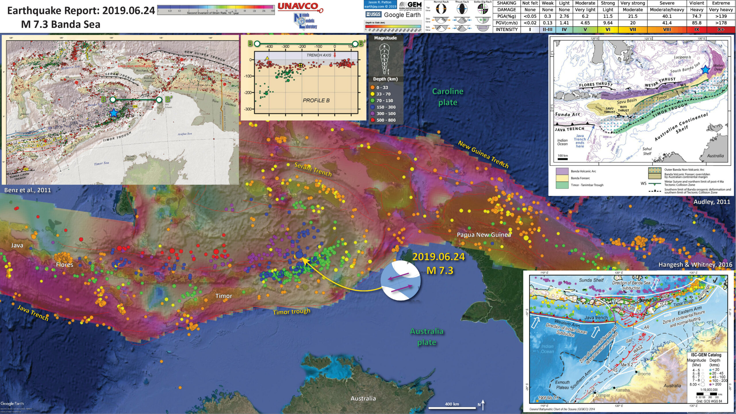
Below is my interpretive poster for this earthquake
I plot the seismicity from the past month, with color representing depth and diameter representing magnitude (see legend). I include earthquake epicenters from 1919-2019 with magnitudes M ≥ 7.0 in one version.
I plot the USGS fault plane solutions (moment tensors in blue and focal mechanisms in orange), possibly in addition to some relevant historic earthquakes. Some earthquakes have older focal mechanisms plotted in black and white.
- I placed a moment tensor / focal mechanism legend on the poster. There is more material from the USGS web sites about moment tensors and focal mechanisms (the beach ball symbols). Both moment tensors and focal mechanisms are solutions to seismologic data that reveal two possible interpretations for fault orientation and sense of motion. One must use other information, like the regional tectonics, to interpret which of the two possibilities is more likely.
- I also include the shaking intensity contours on the map. These use the Modified Mercalli Intensity Scale (MMI; see the legend on the map). This is based upon a computer model estimate of ground motions, different from the “Did You Feel It?” estimate of ground motions that is actually based on real observations. The MMI is a qualitative measure of shaking intensity. More on the MMI scale can be found here and here. This is based upon a computer model estimate of ground motions, different from the “Did You Feel It?” estimate of ground motions that is actually based on real observations.
- I include the slab 2.0 contours plotted (Hayes, 2018), which are contours that represent the depth to the subduction zone fault. These are mostly based upon seismicity. The depths of the earthquakes have considerable error and do not all occur along the subduction zone faults, so these slab contours are simply the best estimate for the location of the fault.
- In the map below, I include a transparent overlay of the magnetic anomaly data from EMAG2 (Meyer et al., 2017). As oceanic crust is formed, it inherits the magnetic field at the time. At different points through time, the magnetic polarity (north vs. south) flips, the North Pole becomes the South Pole. These changes in polarity can be seen when measuring the magnetic field above oceanic plates. This is one of the fundamental evidences for plate spreading at oceanic spreading ridges (like the Gorda rise).
- Regions with magnetic fields aligned like today’s magnetic polarity are colored red in the EMAG2 data, while reversed polarity regions are colored blue. Regions of intermediate magnetic field are colored light purple.
- We can see the roughly east-west trends of these red and blue stripes in the Caroline and Australia plates. These lines are parallel to the ocean spreading ridges from where they were formed. The stripes disappear at the subduction zone because the oceanic crust with these anomalies is diving deep beneath the Sunda plate (part of Eurasia), so the magnetic anomalies from the overlying Sunda plate mask the evidence for the Australia plate.
Magnetic Anomalies
- In a map below, I include a transparent overlay of the Global Strain Rate Map (Kreemer et al., 2014).
- The mission of the Global Strain Rate Map (GSRM) project is to determine a globally self-consistent strain rate and velocity field model, consistent with geodetic and geologic field observations. The overall mission also includes:
- contributions of global, regional, and local models by individual researchers
- archive existing data sets of geologic, geodetic, and seismic information that can contribute toward a greater understanding of strain phenomena
- archive existing methods for modeling strain rates and strain transients
- The completed global strain rate map will provide a large amount of information that is vital for our understanding of continental dynamics and for the quantification of seismic hazards.
- The version used in the poster(s) below is an update to the original 2004 map (Kreemer et al., 2000, 2003; Holt et al., 2005).
Global Strain
- In the upper left corner, I include a map from Benz et al. (2011) that shows historic earthquake locations (epicenters) along with some of the plate boundary faults. Note the strike slip fault (with the opposing black arrows) that cross the location of the 1938 earthquake (labeled in yellow on that map). I placed a blue star in the location of the M 7.3 quake. There is a cross section to the right of the map that shows how earthquakes dive down with a westward trend (following the plate down the subduction zone). The cross section location is shown on the map (B-B’).
- In the upper right corner is a larger scale tectonic map from Audley (2011) showing the major thrust faults and the large forearc basin is labeled “Weber Deep.”
- Hangesh and Whitney (2016) did lots of work on the faulting in the region to the south of the M 7.3. They show block boundaries and relative plate motion arrows in white. Note how they extend strike-slip motion along the Timor trough. This may be in addition to the strike-slip along the backthrust.
I include some inset figures. Some of the same figures are located in different places on the larger scale map below.
- Here is the map with a month’s seismicity plotted. I included MMI contours from a recent M 6.3 earthquake in PNG, which led to a sequence of additional M~6 quakes to the southeast of that main shock. I won’t be writing a report for those quakes, even though it is interesting (check it out!). Sorry to have misspelled Hengesh as Hangesh.

- Here is the map with a century’s seismicity (M ≥ 7.0) plotted.

- Here is the map with a month’s seismicity (M ≥ 0.5) plotted with the Global Strain data plotted. We can see the 2018 Flores swarm show up here.

Other Report Pages
Some Relevant Discussion and Figures
- Here is a tectonic map for this part of the world from Zahirovic et al., 2014. They show a fracture zone where the M 7.3 earthquake happened. I left out all the acronym definitions (you’re welcome), but they are listed in the paper.

Regional tectonic setting with plate boundaries (MORs/transforms = black, subduction zones = teethed red) from Bird (2003) and ophiolite belts representing sutures modified from Hutchison (1975) and Baldwin et al. (2012). West Sulawesi basalts are from Polvé et al. (1997), fracture zones are from Matthews et al. (2011) and basin outlines are from Hearn et al. (2003).
- This is a great visualization showing the Australia plate and how it formed the largest forearc basin on Earth (Pownall et al., 2014).
- The maps on the left show a time history of the tectonics. The low angle oblique view on the right shows the dipping crust (north is not always up, as in this figure).
- In the lower right, they show how there is strike-slip faulting along the Seram trough also (I left out the figure caption for E).

Reconstructions of eastern Indonesia, adapted from Hall (2012), depict collision of Australia with Southeast Asia and slab rollback into Banda Embayment. Yellow star indicates Seram. Oceanic crust is shown in purple (older than 120 Ma) and blue (younger than 120 Ma); submarine arcs and oceanic plateaus are shown in cyan; volcanic island arcs, ophiolites, and material accreted along plate margins are shown in green. A: Reconstruction at 15 Ma. B: Reconstruction at 7 Ma. C: Reconstruction at 2 Ma. D: Visualization of present-day slab morphology of proto–Banda Sea based on earthquake hypocenter distribution and tomographic models
- Here is a map and some cross sections showing seismic tomography (like C-T scans into the Earth using seismic waves instead of X-Rays). The map shows the location of the cross sections (Spakman et al., 2010).

The Banda arc and surrounding region. 200 m and 4,000 m bathymetric contours are indicated. The numbered black lines are Benioff zone contours in kilometres. The red triangles are Holocene volcanoes (http://www.volcano.si.edu/world/). Ar=Aru, Ar Tr=Aru trough, Ba=Banggai Islands, Bu=Buru, SBS=South Banda Sea, Se=Seram, Sm=Sumba, Su=Sula Islands, Ta=Tanimbar, Ta Tr=Tanimbar trough, Ti=Timor, W=Weber Deep.

Tomographic images of the Banda slab. Vertical sections through the tomography model along the lines shown in Fig. 1. Colours: P-wave anomalies with reference to velocity model ak135 (ref. 30). Dots: earthquake hypocentres within 12 km of the section. The dashed lines are phase changes at ~410 km and ~660 km. The sections are plotted without vertical exaggeration; the horizontal axis is in degrees. The labelled positive anomalies are the Sunda (Su) and Banda (Ba) slabs: BuDdetached slab under Buru, FlDslab under Flores, SDslab under Seram, TDslab under Timor. a, The Sunda slab enters the lower mantle whereas the Banda embayment slab is entirely in the upper mantle with the change under Sulawesi. b–e, Banda slab morphology in sections parallel to Australia plate motion shows a transition from a steep slab with a flat section (fs) (b) to a spoon shape shallowing eastward (c–e).
- Here is the map from Benz et al. (2011).

- Here is the tectonic map from Hengesh and Whitney (2016)

Illustration of major tectonic elements in triple junction geometry: tectonic features labeled per Figure 1; seismicity from ISC-GEM catalog [Storchak et al., 2013]; faults in Savu basin from Rigg and Hall [2011] and Harris et al. [2009]. Purple line is edge of Australian continental basement and fore arc [Rigg and Hall, 2011]. Abbreviations: AR = Ashmore Reef; SR = Scott Reef; RS = Rowley Shoals; TCZ = Timor Collision Zone; ST = Savu thrust; SB = Savu Basin; TT = Timor thrust; WT =Wetar thrust; WASZ = Western Australia Shear Zone. Open arrows indicate relative direction of motion; solid arrows direction of vergence.
- Here is the Audley (2011) cross section showing how the backthrust relates to the subduction zone beneath Timor. I include their figure caption in blockquote below.

Cartoon cross section of Timor today, (cf. Richardson & Blundell 1996, their BIRPS figs 3b, 4b & 7; and their fig. 6 gravity model 2 after Woodside et al. 1989; and Snyder et al. 1996 their fig. 6a). Dimensions of the filled 40 km deep present-day Timor Tectonic Collision Zone are based on BIRPS seismic, earthquake seismicity and gravity data all re-interpreted here from Richardson & Blundell (1996) and from Snyder et al. (1996). NB. The Bobonaro Melange, its broken formation and other facies are not indicated, but they are included with the Gondwana mega-sequence. Note defunct Banda Trench, now the Timor TCZ, filled with Australian continental crust and Asian nappes that occupy all space between Wetar Suture and the 2–3 km deep deformation front north of the axis of the Timor Trough. Note the much younger decollement D5 used exactly the same part of the Jurassic lithology of the Gondwana mega-sequence in the older D1 decollement that produced what appears to be much stronger deformation.
- Here is a figure showing the regional geodetic motions (Bock et al., 2003). I include their figure caption below as a blockquote.

Topographic and tectonic map of the Indonesian archipelago and surrounding region. Labeled, shaded arrows show motion (NUVEL-1A model) of the first-named tectonic plate relative to the second. Solid arrows are velocity vectors derived from GPS surveys from 1991 through 2001, in ITRF2000. For clarity, only a few of the vectors for Sumatra are included. The detailed velocity field for Sumatra is shown in Figure 5. Velocity vector ellipses indicate 2-D 95% confidence levels based on the formal (white noise only) uncertainty estimates. NGT, New Guinea Trench; NST, North Sulawesi Trench; SF, Sumatran Fault; TAF, Tarera-Aiduna Fault. Bathymetry [Smith and Sandwell, 1997] in this and all subsequent figures contoured at 2 km intervals.
- Whitney and Hengesh (2015) used GPS modeling to suggest a model of plate blocks. Below are their model results.

Plate boundary segments in the Banda Arc region from Nugroho et al (2009). Numbers inside rectangles show possible micro-plate blocks near the Sumba Triple Junction (colored) based on GPS velocities (black arrows) with in a stable Eurasian reference frame.
- Here is the conceptual model from Whitney and Hengesh (2015) that shows how left-lateral strike-slip faulting can come into the region.
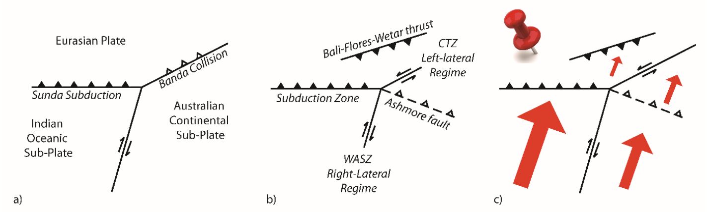
Schematic map views of kinematic relations between major crustal elements in the Sumba Triple Junction region. CTZ= collisional tectonic zone. Red arrow size designates schematic plate motion relations based on geological data relative to a fixed Sunda shelf reference frame (pin).
Geologic Fundamentals
- For more on the graphical representation of moment tensors and focal mechanisms, check this IRIS video out:
- Here is a fantastic infographic from Frisch et al. (2011). This figure shows some examples of earthquakes in different plate tectonic settings, and what their fault plane solutions are. There is a cross section showing these focal mechanisms for a thrust or reverse earthquake. The upper right corner includes my favorite figure of all time. This shows the first motion (up or down) for each of the four quadrants. This figure also shows how the amplitude of the seismic waves are greatest (generally) in the middle of the quadrant and decrease to zero at the nodal planes (the boundary of each quadrant).

- Here is another way to look at these beach balls.
The two beach balls show the stike-slip fault motions for the M6.4 (left) and M6.0 (right) earthquakes. Helena Buurman's primer on reading those symbols is here. pic.twitter.com/aWrrb8I9tj
— AK Earthquake Center (@AKearthquake) August 15, 2018
- There are three types of earthquakes, strike-slip, compressional (reverse or thrust, depending upon the dip of the fault), and extensional (normal). Here is are some animations of these three types of earthquake faults. The following three animations are from IRIS.
Strike Slip:
Compressional:
Extensional:
- This is an image from the USGS that shows how, when an oceanic plate moves over a hotspot, the volcanoes formed over the hotspot form a series of volcanoes that increase in age in the direction of plate motion. The presumption is that the hotspot is stable and stays in one location. Torsvik et al. (2017) use various methods to evaluate why this is a false presumption for the Hawaii Hotspot.
- Here is a map from Torsvik et al. (2017) that shows the age of volcanic rocks at different locations along the Hawaii-Emperor Seamount Chain.
- Here is a great tweet that discusses the different parts of a seismogram and how the internal structures of the Earth help control seismic waves as they propagate in the Earth.

A cutaway view along the Hawaiian island chain showing the inferred mantle plume that has fed the Hawaiian hot spot on the overriding Pacific Plate. The geologic ages of the oldest volcano on each island (Ma = millions of years ago) are progressively older to the northwest, consistent with the hot spot model for the origin of the Hawaiian Ridge-Emperor Seamount Chain. (Modified from image of Joel E. Robinson, USGS, in “This Dynamic Planet” map of Simkin and others, 2006.)

Hawaiian-Emperor Chain. White dots are the locations of radiometrically dated seamounts, atolls and islands, based on compilations of Doubrovine et al. and O’Connor et al. Features encircled with larger white circles are discussed in the text and Fig. 2. Marine gravity anomaly map is from Sandwell and Smith.
Today, on #SeismogramSaturday: what are all those strangely-named seismic phases described in seismograms from distant earthquakes? And what do they tell us about Earth’s interior? pic.twitter.com/VJ9pXJFdCy
— Jackie Caplan-Auerbach (@geophysichick) February 23, 2019
- M 9.2 Andaman-Sumatra subduction zone 2014 Earthquake Anniversary
- M 9.2 Andaman-Sumatra subduction zone SASZ Fault Deformation
- M 9.2 Andaman-Sumatra subduction zone 2016 Earthquake Anniversary
- 2019.06.23 M 7.3 Banda Sea
- 2019.04.12 M 6.8 Sulawesi, Indonesia
- 2018.09.28 M 7.5 Sulawesi
- 2018.10.16 M 7.5 Sulawesi UPDATE #1
- 2018.08.19 M 6.9 Lombok, Indonesia
- 2018.08.05 M 6.9 Lombok, Indonesia
- 2018.07.28 M 6.4 Lombok, Indonesia
- 2017.12.15 M 6.5 Java
- 2017.08.31 M 6.3 Mentawai, Sumatra
- 2017.08.13 M 6.4 Bengkulu, Sumatra, Indonesia
- 2017.05.29 M 6.8 Sulawesi, Indonesia
- 2017.03.14 M 6.0 Sumatra
- 2017.03.01 M 5.5 Banda Sea
- 2016.10.19 M 6.6 Java
- 2016.03.02 M 7.8 Sumatra/Indian Ocean
- 2015.07.22 M 5.8 Andaman Sea
- 2015.11.08 M 6.4 Nicobar Isles
- 2012.04.11 M 8.6 Sumatra outer rise
- 2004.12.26 M 9.2 Andaman-Sumatra subduction zone
Indonesia | Sumatra
General Overview
Earthquake Reports
Social Media
- Audley-Charles, M.G., 1986. Rates of Neogene and Quaternary tectonic movements in the Southern Banda Arc based on micropalaeontology in: Journal of fhe Geological Society, London, Vol. 143, 1986, pp. 161-175.
- Audley-Charles, M.G., 2011. Tectonic post-collision processes in Timor, Hall, R., Cottam, M. A. &Wilson, M. E. J. (eds) The SE Asian Gateway: History and Tectonics of the Australia–Asia Collision. Geological Society, London, Special Publications, 355, 241–266.
- Baldwin, S.L., Fitzgerald, P.G., and Webb, L.E., 2012. Tectonics of the New Guinea Region in Annu. Rev. Earth Planet. Sci., v. 41, p. 485-520.
- Benz, H.M., Herman, Matthew, Tarr, A.C., Hayes, G.P., Furlong, K.P., Villaseñor, Antonio, Dart, R.L., and Rhea, Susan, 2011. Seismicity of the Earth 1900–2010 New Guinea and vicinity: U.S. Geological Survey Open-File Report 2010–1083-H, scale 1:8,000,000.
- Given, J. W., and H. Kanamori (1980). The depth extent of the 1977 Sumbawa, Indonesia, earthquake, in EOS Trans. AGU., v. 61, p. 1044.
- Gusnman, A.R., Tanioka, Y., Matsumoto, H., and Iwasakai, S.-I., 2009. Analysis of the Tsunami Generated by the Great 1977 Sumba Earthquake that Occurred in Indonesia in BSSA, v. 99, no. 4, p. 2169-2179, https://doi.org/10.1785/0120080324
- Hall, R., 2011. Australia-SE Asia collision: plate tectonics and crustal flow in Geological Society, London, Special Publications 2011; v. 355; p. 75-109 doi: 10.1144/SP355.5
- Hangesh, J. and Whitney, B., 2014. Quaternary Reactivation of Australia’s Western Passive Margin: Inception of a New Plate Boundary? in: 5th International INQUA Meeting on Paleoseismology, Active Tectonics and Archeoseismology (PATA), 21-27 September 2014, Busan, Korea, 4 pp.
- Frisch, W., Meschede, M., Blakey, R., 2011. Plate Tectonics, Springer-Verlag, London, 213 pp.
- Hayes, G., 2018, Slab2 – A Comprehensive Subduction Zone Geometry Model: U.S. Geological Survey data release, https://doi.org/10.5066/F7PV6JNV.
- Holt, W. E., C. Kreemer, A. J. Haines, L. Estey, C. Meertens, G. Blewitt, and D. Lavallee (2005), Project helps constrain continental dynamics and seismic hazards, Eos Trans. AGU, 86(41), 383–387, , https://doi.org/10.1029/2005EO410002. /li>
- Kreemer, C., J. Haines, W. Holt, G. Blewitt, and D. Lavallee (2000), On the determination of a global strain rate model, Geophys. J. Int., 52(10), 765–770.
- Kreemer, C., W. E. Holt, and A. J. Haines (2003), An integrated global model of present-day plate motions and plate boundary deformation, Geophys. J. Int., 154(1), 8–34, , https://doi.org/10.1046/j.1365-246X.2003.01917.x.
- Kreemer, C., G. Blewitt, E.C. Klein, 2014. A geodetic plate motion and Global Strain Rate Model in Geochemistry, Geophysics, Geosystems, v. 15, p. 3849-3889, https://doi.org/10.1002/2014GC005407.
- Meyer, B., Saltus, R., Chulliat, a., 2017. EMAG2: Earth Magnetic Anomaly Grid (2-arc-minute resolution) Version 3. National Centers for Environmental Information, NOAA. Model. https://doi.org/10.7289/V5H70CVX
- Müller, R.D., Sdrolias, M., Gaina, C. and Roest, W.R., 2008, Age spreading rates and spreading asymmetry of the world’s ocean crust in Geochemistry, Geophysics, Geosystems, 9, Q04006, https://doi.org/10.1029/2007GC001743
- Okal, E. A., & Reymond, D., 2003. The mechanism of great Banda Sea earthquake of 1 February 1938: applying the method of preliminary determination of focal mechanism to a historical event in EPSL, v. 216, p. 1-15.
- Osada, M. and Abe, K., 1981. Mechanism and tectonic implications of the great Banda Sea earthquake of November 4, 1963 in Physics of the Earth and Plentary Interiors, v. 25, p. 129-139
- Pownall, J.M., Hall, R., Armstrong,, R.A., and Forster, M.A., 2014. Earth’s youngest known ultrahigh-temperature granulites discovered on Seram, eastern Indonesia in Geology, v. 42, no. 4, p. 379-282, https://doi.org/10.1130/G35230.1
- Spakman, W. and Hall, R., 2010. Surface deformation and slab–mantle interaction during Banda arc subduction rollback in Nature Geosceince, v. 3, p. 562-566, https://doi.org/10.1038/NGEO917
- Whitney, B.B. and Hengesh, J.V., 2015. A new model for active intraplate tectonics in western Australia in Proceedings of the Tenth Pacific Conference on Earthquake Engineering Building an Earthquake-Resilient Pacific 6-8 November 2015, Sydney, Australia, paper number 82
- Zahirovic, S., Seton, M., and Müller, R.D., 2014. The Cretaceous and Cenozoic tectonic evolution of Southeast Asia in Solid Earth, v. 5, p. 227-273, doi:10.5194/se-5-227-2014
References:
Return to the Earthquake Reports page.