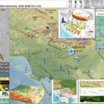
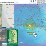
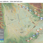
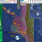
Late last night there was a sequence of earthquakes in southern California. The mainshock is a M 4.5 earthquake.
https://earthquake.usgs.gov/earthquakes/eventpage/ci38695658/executive
This temblor was widely felt across the southland (including by my mom, who was warned by earthquake early warning). This sequence happened in the same area as the 1987 Whittier Narrows Earthquake Sequence (which I felt as a child, growing up in Long Beach, CA).
https://earthquake.usgs.gov/earthquakes/eventpage/ci731691/executive
The tectonics of southern CA are dominated by the San Andreas fault (SAF) system. The SAF system is a right-lateral strike-slip plate boundary fault marking the boundary between the Pacific and North America plates.
Basically, the Pacific plate is moving northwest relative to the North America plate. Both plates are moving northwest relative to an Earth reference frame, but the Pacific plate is moving faster.
The SAF system goes through a bend in southern CA, which causes things to get complicated. There are sibling faults to the SAF, also right-lateral strike-slip (e.g. the San Jacinto and Elsinore faults).
Also, because of the fault geometry, there is considerable north-south compression that forms the mountain ranges to the north of the Los Angeles Basin. Some of the faults formed by this compression are the Sierra Madre, Hollywood, Compton, and Puente Hills faults.
A recent earthquake (2014) happened along one of these thrust fault systems. On 28 March 2014 (one day after the 50th anniversary of the Good Friday Earthquake in Alaska) there was an oblique thrust fault earthquake beneath La Habra, CA. My cousins felt that sequence and I remember them mentioning how their children kept waking up after every aftershock, some epicenters were located within a half km from their house.
https://earthquake.usgs.gov/earthquakes/eventpage/ci15481673/executive
This La Habra sequence appears to be related to the Puente Hills Thrust fault system (same for the Whittier Narrows Earthquake). Last night’s M 4.5 also appears to have slipped along a thrust fault on this system. Based on the depth, it looks like the earthquake slipped along the Lower Elysian Park ramp (see poster).
There were a few aftershocks. However, two of them I would rather interpret them as triggered earthquakes. The M 1.6 and M 1.9 earthquakes have strike-slip earthquake mechanisms (focal mechanisms = orange). These also have shallower [hypocentral] depths. There is mapped the Montebello fault, a right-lateral strike-slip fault, just to the east of the M 4.5 epicenter. The Montebello fault is a strand of the Whittier fault system.
So, while this may be incorrect, my initial interpretation is that these two M1+ events happened on the Montebello fault system and were triggered by the M 4.5 event.
There was also an historic earthquake on the Sierra Madre fault system. On 28 June 1991, there was a M 5.8 earthquake beneath the San Gabriel Mountains to the north of the LA Basin. This was also an oblique thrust earthquake.
https://earthquake.usgs.gov/earthquakes/eventpage/ci2021449/executive
Something that all these earthquakes share is that they occurred on blind thrust faults. Why are they called blind? Because they don’t reach the ground surface, so we cannot see them at the surface (thus, we are blind to them).
Below is my interpretive poster for this earthquake
- I plot the seismicity from the past month, with diameter representing magnitude (see legend). I include earthquake epicenters from 1920-2020 with magnitudes M ≥ 4.5.
- I plot the USGS fault plane solutions (moment tensors in blue and focal mechanisms in orange), possibly in addition to some relevant historic earthquakes.
- A review of the basic base map variations and data that I use for the interpretive posters can be found on the Earthquake Reports page.
- Some basic fundamentals of earthquake geology and plate tectonics can be found on the Earthquake Plate Tectonic Fundamentals page.
- In the upper left corner I include a map that shows the USGS tectonic faults and the USGS seismicity from the past 3 months. I highlight the North America and Pacific plates and their relative motion along the San Andreas fault system.
- In the lower right corner I plot the epicenters related to this sequence. The topographic data here are high resolution LiDAR data from 2016 (publically available).
- In the lower center left is a low-angle oblique block diagram from Daout at al. (2016) that shows the geometry of the major faults in this area (along with estimates of the slip rates for these faults).
- Between the aftershock map and the oblique block diagram are two panels from Rollins et al. (2018). On the left is a map that shows the major fault systems, some historic earthquake mechanisms, and GPS derived plate motion vectors (the direction of relative motion is the orientation of the arrow and the velocity is the length of the arrow). I placed a blue star in the location of last night’s M 4.5. On the right are some cross sections through the subsurface (the location of these cross sections is shown as a dashed gray line on the map). The M 4.5 hypocentral depth is 16.9 km, which clearly plots on the Lower Elysian Park ramp (part of the Puente Hills fault system). Note how the Whittier fault, a strike-slip fault at the surface, soles into the Peunte Hills thrus.
- In the upper right corner is a map where I plot a comparison of the CSIN intensity model results (using the MMI Intensity scale, read more about that here) and the USGS “Did You Feel It?” (dyfi) reports. The intensity map is based on a model of how intensity diminishes with distance from the earthquake. The dyfi results are from real observations from real people. See the plot below the map to check out how these data compare, but in a plot not a map.
- To the left of the intensity comparisons is another map from Rollins et al. (2018) that shows how much these thrust fault systems are accumulating energy over time. Basically, the warmer colors (e.g. red) shows an area of the fault that is storing more energy per year relative to part of the fault that have less warm colors (e.g. yellow). The Sierra Madre fault system is storing the most energy, per year, of all thrust faults that Rollins and his colleagues studied.
I include some inset figures. Some of the same figures are located in different places on the larger scale map below.
- Two of the most notable historic earthquakes in southern CA are the 1971 Sylmar and 1994 Northridge earthquakes. Both earthquakes had a significant impact on the growth of knowledge about earthquake hazards in southern CA (and elsewhere), but they also resulted in major changes in how seismic hazards are recognized, codified, and mitigated throughout the state (with impacts nationwide and worldwide). And, both of these earthquakes also happened on blind thrust faults, just like last night’s M 4.5!
- The 1906 San Francisco and 1933 Long Beach earthquakes led to major changes in the state too. 1933 Long Beach particularly led to changes in how schools are built and resulted in the strongest building code (relative to earthquakes) in the country as the time. These changes were eventually adopted statewide, nationwide, and globally (via the universal building code). Check out the Field Act to learn more about this.
- The 1971 Sylmar Earthquake happened on a previously unrecognized fault (because it is blind) and caused lots of damage and many casualties. Perhaps most notably was the veterans hospital which was built across a fault. This fault slipped during the earthquake (triggered by the mainshock). Because the fault slipped beneath the hospital, the hospital was cut in half.
- This was quite educational, to learn that when an earthquake fault slips beneath a building, the building does not (generally) perform well. After this earthquake, state senators Alquist and Priolo wrote and helped to get passed the Alquist-Priolo Act. This act required the state (via the California Geological Survey (CGS), where I work) to identify all active faults in the state. The Board of Mines and Geology (BMG) prepared regulations that help manage development (i.e. construction of buildings) in AP zones. Read more about the AP Act here.
- The 1994 Northridge Earthquake, with a similar magnitude as the 1971 Sylmar quake, caused extensive damage throughout the San Fernando Valley (like, totally dude) and beyond. There are famous photos of the damage to bridges of the 5 and 14 interchange (interstate 5 and state route 14). The 1994 Northridge Earthquake led to the development of the Seismic Hazards Mapping Act. The CGS and the BMG both have mandates related to the SHMA (I work as part of the Seismic Hazards Mapping Program at CGS). Read more about the SHMA here.
- Read more about the 1971 Sylmar Earthquake here.
- Read more about the 1994 Northridge Earthquake here.
Other Report Pages
Some Relevant Discussion and Figures
- Here is a great map from Wallace (1990) that shows the major faults associated with the San Andreas fault system.
Generalized topographic map of southern California, showing major faults with Quaternary activity in the San Andreas firnit system. Faults dotted where concealed by water: hachures on contours indicate area of closed low.
- This is a more updated map from Tucker and Dolan (2001) prepared for their study of the Sierra Madre fault.
Regional neotectonic map for metropolitan southern California showing major active faults. The Sierra Madre fault is a 75-km-long active reverse fault that extends along the northern edge of the metropolitan region. Fault locations are from Ziony and Jones (1989), Vedder et al. (1986), Dolan and Sieh (1992), Sorlien (1994), and Dolan et al. (1997, 2000b). Closed teeth denote reverse fault surface trace; open teeth on dashed lines show upper edge of blind thrust fault ramps. Strike-slip fault surface traces shown by double arrows. Star denotes location of Oak Hill paleoseismologic trench site of Bonilla (1973). CSI, Clamshell-Sawpit fault; ELATB, East Los Angeles blind thrust system; EPT, Elysian park blind thrust fault; Hol Fl, Hollywood fault; PHT, Puente Hills blind thrust fault; RMF, Red Mountain fault; SCII, Santa Cruz Island fault; SSF, Santa Susana fault; SJcF, San Jacinto fault; SJF, San Jose fault; VF, Verdugo fault; A, Altadena study site of Rubin et al. (1998); LA, Los Angeles; LB, Long Beach; LC, La Crescenta; M, Malibu; NB, Newport Beach; Ox, Oxnard; P, Pasadena; PH, Port Hueneme; S, Horsethief Canyon study site in San Dimas; V, Ventura. Dark shading denotes mountains.
- This is a great low angle oblique view of the faults in the southland from Fuis et al. (2001). Note that the SAF geometry creates North-South compression in this area (that causes the thrust faults, some of hem are blind).
Schematic block diagram showing interpreted tectonics in vicinity of LARSE line 1. Active faults are shown in orange, and moderate and large earthquakes are shown with orange stars and attached dates, magnitudes, and names. Gray half-arrows show relative motions on faults. Small white arrows show block motions in vicinities of bright reflective zones A and B (see Fig. 2A). Large white arrows show relative convergence direction of Pacific and North American plates. We interpret a master de´collement ascending from bright reflective zone A at San Andreas fault, above which brittle upper crust is imbricating along thrust and reverse faults and below which lower crust is flowing toward San Andreas fault (brown arrows) and depressing Moho. Fluid injection, indicated by small lenticular blue areas, is envisioned in bright reflective zones A and B.
- This is an updated figure from Daout et al. (2016). The slip rates are included for each fault.
Three-dimensional schematic block model across the SGM [after Fuis et al., 2001b] superimposed to the digital elevation model, the seismicity (yellow dots), the Moho model (red line), and interpreted active faults summarizing the average interseismic strike-slip (back arrows) and dip-slip (red arrows) rates extracted from the Bayesian exploration. Shallow faults (dashed lines) that formed a complex three-dimensional system at the surface [Plesch et al., 2007] are locked during the interseismic period, while the ramp-décollement system (solid lines) decouples the upper crust from the lower crust and partitioned the observed uniform velocity field (blue vector) at the downdip end of the structures.
- Here is a summary of the historic earthquakes in southern CA from Hauksson et al. (1995). They include earthquake mechanisms (B) and the regions impacted (A).
(a) Significant earthquakes of M > 4.8 that have occurred in the greater Los Angeles basin area since 1920. Aftershock zones are shaded with cross hatching, including the 1994 Northridge earthquake. Dotted areas indicate surface rupture, including the rupture of the 1857 earthquake along the San Andreas fault. (b) Lower hemisphere focal mechanisms (shaded quadrants are compressional) for significant earthquakes that have occurred since 1933 in the greater Los Angeles area.
- This is an important figure from Leon et al. (2007) that shows their interpretation of the different faults in the Puente Hills fault system. They highlight the location of the 1987 Whittier Narrows Earthquake, which was to the north of last nights M 4.5.
- This is also an important figure as it shows some additional faults (Shaw et al., 2002). The M 4.5 most likely occurred on the Lower Elysian Park fault.
Structure contour map of the PHT in relation to other major thrust and strike-slip systems in the northern LA basin. Contour interval is 1 km; depths are subsea. Map coordinates are UTM Zone 11, NAD27 datum.
- What follows are a series of figures from Rollins et al. (2018). They studied the strain accumulation (the accumulation of energy in a fault system over time) for the three main thrust fault systems in the LA Basin.
- Here is their first figure that shows the relative plate motions as observed using GPS sites.
- Here is their cross section through this part of the LA Basin. The location of this cross section is marked on the above map as a gray dashed line.
- I love this map because it shows how these thrust faults dip into the Earth to the north.
- Finally, we see how they model the amount of plate tectonic motion is accumulated as tectonic strain on these faults. Chris is one of the smartest plate tectonicists I know, so read his paper (several times).
(a) Tectonics and shortening in the Los Angeles region. Dark blue arrows are shortening-related GPS velocities relative to the San Gabriel Mountains (Argus et al., 2005). Contours are uniaxial strain rate (rate of change of εxx) in the N ~5° E direction estimated from the GPS using the method of Tape et al. (2009). Background shading is the shear modulus at 100-m depth in the CVM*, a heterogeneous elastic model based on the Community Velocity Model (Süss & Shaw, 2003; Shaw et al., 2015) that we create and use in this study (section 4). Black lines are upper edges of faults, dashed for blind faults. Epicenters of the 1971, 1987, and 1994 earthquakes are from Southern California Earthquake Data Center; focal mechanisms are from Heaton (1982) for 1971 and Global CMT Catalog for 1987 and 1994. Profile A-A0 follows LARSE line 1 (Fuis et al., 2001) onshore and line M-M0 of Sorlien et al. (2013) offshore. SGF = San Gabriel Fault; SSF = Santa Susana Fault. VF = Verdugo Fault. SAF = San Andreas Fault. CuF = Cucamonga Fault. A-DF = Anacapa-Dume Fault. SMoF = Santa Monica Fault. HF = Hollywood Fault. RF = Raymond Fault. UEPF = Upper Elysian Park Fault. ChF = Chino Fault. WF = Whittier Fault. N-IF = Newport-Inglewood Fault. PVF = Palos Verdes Fault. (b) GPS velocities on islands. (c) Tectonic setting. Black lines and pairs of half-arrows, respectively, are major faults and their slip senses. Black arrow is Pacific Plate velocity relative to North American plate from Kreemer et al. (2014). GF = Garlock Fault. SJF = San Jacinto Fault. EF = Elsinore Fault. SB = Santa Barbara. LA = Los Angeles. SD = San Diego.
(a) Cross sections of faults, structure, north-south contraction, and seismicity along profile A-A0 . Red lines are fault surfaces as meshed here (Figure 3), dashed where uncertain (Shaw & Suppe, 1996; Shaw & Shearer, 1999; Fuis et al., 2012). Geometries of basin, basement, and mantle are from Shaw et al. (2015); geometry of base of Fernando Formation (boundary between beige and tan units of the basin) is interpolated from Sorlien et al. (2013; offshore), Wright (1991; coastline to Whittier Fault), and Yeats (2004; Whittier Fault to Sierra Madre Fault); topography is from Fuis et al. (2012). (b) Projections of Argus et al. (2005) GPS velocities (relative to San Gabriel Mountains) onto the direction N 5° E and 1σ uncertainties. Note that stations on Palos Verdes are plotted left of the coastline as the offshore section of profile A-A0 passes alongside Palos Verdes (Figure 1a). (c) Seismotectonic features. Distribution of shear modulus is from the CVM*, the heterogeneous elastic model used in this study (section 4). Translucent white circles are relocated 1981–2016 M ≥ 2 earthquakes whose epicenters lie within the mesh area of the three thrust faults and decollement (Hauksson et al., 2012 and updated). PVF = Palos Verdes Fault; N-IF = Newport-Inglewood Fault; WF = Whittier Fault.
geometries of the three main thrust faults beneath the Los Angeles basin (section 4), colored by depth, and 1981–2016 M ≥ 2.5 earthquakes within the mesh area from Hauksson et al. (2012 and updated), scaled by magnitude (white-filled circles). Gray-filled circles are 1981–2016 M ≥ 4.5 earthquakes outside the mesh area. Inferred paleoearthquakes are from Rubin et al. (1998) and Leon et al. (2007, 2009). SAF = San Andreas Fault.
Estimates of moment deficit accumulation rate from combining the four interseismic strain accumulation models. (a) Spatial distribution of moment deficit accumulation rate per area. (Values are on the order of ~108 N m -1 yr -1 as the moment deficit accumulation rate per patch is on the order of 1015 N m -1 yr -1 [Figure S11] and the patches are a few kilometers (a few thousand meters) on a side.) (b) Unified PDF of moment deficit accumulation rate (dark blue object) formed by combining the PDFs from the four strain accumulation models. The PDF would follow the red curve if strain accumulation updip of the tips of the Puente Hills and Compton faults (PHF and CF) were counted.
- 1906.04.18 M 7.9 San Francisco
- 2017.12.14 M 4.3 Laytonville
- 2016.11.06 M 4.1 Laytonville, CA
- 2016.11.03 M 3.8 Laytonville, CA
- 2016.08.10 M 5.1 Lake Pillsbury, CA
- 2016.08.04 M 4.5 Honey Lake, CA
- 2015.08.30 M 3.6 Mendocino County, CA
- 2015.07.27 M 3.5 Point Arena, CA
- 2018.07.30 M 3.7 San Pablo Bay
- 2018.01.04 M 4.4 Berkeley
- 1989.10.18 M 6.9 Loma Prieta
- 2020.09.19 M 4.5 El Monte
- 2020.06.24 M 5.8 Lone Pine
- 2019.07.04 M 6.4 Ridgecrest
- 2019.07.05 M 6.4 / 7.1 Ridgecrest Update #1
- 2019.07.18 M 6.4 / 7.1 Ridgecrest Update #2
- 2019.07.20 M 6.4 / 7.1 Ridgecrest Update #3
- 2019.06.05 M 4.3 San Clemente Island
- 2018.04.05 M 5.3 Channel Islands
- 2018.04.05 M 5.3 Channel Islands Update #1
- 2016.02.23 M 4.9 Bakersfield
- 2015.12.30 M 4.4 San Bernardino, CA
- 2015.05.03 M 3.8 Los Angeles, CA
- 2015.04.13 M 3.3 Los Angeles, CA
- 2014.04.01 M 5.1 La Habra p-3
- 2014.03.29 M 5.1 La Habra p-2
- 2014.03.28 M 5.1 La Habra p-1
- 1994.11.17 M 6.7 Northridge, CA
- 1971.02.09 M 6.7 Sylmar, CA
- Frisch, W., Meschede, M., Blakey, R., 2011. Plate Tectonics, Springer-Verlag, London, 213 pp.
- Hayes, G., 2018, Slab2 – A Comprehensive Subduction Zone Geometry Model: U.S. Geological Survey data release, https://doi.org/10.5066/F7PV6JNV.
- Holt, W. E., C. Kreemer, A. J. Haines, L. Estey, C. Meertens, G. Blewitt, and D. Lavallee (2005), Project helps constrain continental dynamics and seismic hazards, Eos Trans. AGU, 86(41), 383–387, , https://doi.org/10.1029/2005EO410002. /li>
- Jessee, M.A.N., Hamburger, M. W., Allstadt, K., Wald, D. J., Robeson, S. M., Tanyas, H., et al. (2018). A global empirical model for near-real-time assessment of seismically induced landslides. Journal of Geophysical Research: Earth Surface, 123, 1835–1859. https://doi.org/10.1029/2017JF004494
- Kreemer, C., J. Haines, W. Holt, G. Blewitt, and D. Lavallee (2000), On the determination of a global strain rate model, Geophys. J. Int., 52(10), 765–770.
- Kreemer, C., W. E. Holt, and A. J. Haines (2003), An integrated global model of present-day plate motions and plate boundary deformation, Geophys. J. Int., 154(1), 8–34, , https://doi.org/10.1046/j.1365-246X.2003.01917.x.
- Kreemer, C., G. Blewitt, E.C. Klein, 2014. A geodetic plate motion and Global Strain Rate Model in Geochemistry, Geophysics, Geosystems, v. 15, p. 3849-3889, https://doi.org/10.1002/2014GC005407.
- Meyer, B., Saltus, R., Chulliat, a., 2017. EMAG2: Earth Magnetic Anomaly Grid (2-arc-minute resolution) Version 3. National Centers for Environmental Information, NOAA. Model. https://doi.org/10.7289/V5H70CVX
- Müller, R.D., Sdrolias, M., Gaina, C. and Roest, W.R., 2008, Age spreading rates and spreading asymmetry of the world’s ocean crust in Geochemistry, Geophysics, Geosystems, 9, Q04006, https://doi.org/10.1029/2007GC001743
- Pagani,M. , J. Garcia-Pelaez, R. Gee, K. Johnson, V. Poggi, R. Styron, G. Weatherill, M. Simionato, D. Viganò, L. Danciu, D. Monelli (2018). Global Earthquake Model (GEM) Seismic Hazard Map (version 2018.1 – December 2018), DOI: 10.13117/GEM-GLOBAL-SEISMIC-HAZARD-MAP-2018.1
- Silva, V ., D Amo-Oduro, A Calderon, J Dabbeek, V Despotaki, L Martins, A Rao, M Simionato, D Viganò, C Yepes, A Acevedo, N Horspool, H Crowley, K Jaiswal, M Journeay, M Pittore, 2018. Global Earthquake Model (GEM) Seismic Risk Map (version 2018.1). https://doi.org/10.13117/GEM-GLOBAL-SEISMIC-RISK-MAP-2018.1
- Zhu, J., Baise, L. G., Thompson, E. M., 2017, An Updated Geospatial Liquefaction Model for Global Application, Bulletin of the Seismological Society of America, 107, p 1365-1385, https://doi.org/0.1785/0120160198
- Daout, S., S. Barbot, G. Peltzer, M.-P. Doin, Z. Liu, and R. Jolivet, 2016. Constraining the kinematics of metropolitan Los Angeles faults with a slip-partitioning model, Geophys. Res. Lett., 43, p. 11,192–11,201 doi:10.1002/2016GL071061.
- Fuis, G.S., Ryberg, T., Godfrey, N.J., Okaya, D.A., and Murphy, J.M., 2001. Crustal structure and tectonics from the Los Angeles basin to the Mojave Desert, southern California in Geology, v. 29, no. 1, p. 15-18
- Hauksson, E., Jones, L.M., and Huttn,K., 1995. The 1994 Northridge earthquake sequence in California: Seismological and tectonic aspects in JGR, v. 100, no. B7, p. 12,235-12,255
- Leon, L. A., S. A. Christofferson, J. F. Dolan, J. H. Shaw, and T. L. Pratt, 2007. Earthquake-by-earthquake fold growth above the Puente Hills blind thrust fault, Los Angeles, California: Implications for fold kinematics and seismic hazard, J. Geophys. Res., 112, B03S03, doi:10.1029/2006JB004461.
- Rollins, C., Avouac, J.-P., Landry, W., Argus, D. F., & Barbot, S., 2018. Interseismic strain accumulation on faults beneath Los Angeles, California. Journal of Geophysical Research: Solid Earth, 123. https://doi.org/10.1029/2017JB015387
- Shaw, J.H., Plesch, A., Dolan,. J.F., Pratt, T.L., and Fiore, P/, 2002. Puente Hills Blind-Thrust System, Los Angeles, California in BSSA v. 92, no. 8,pp. 2946-2960
- Tucker, A.Z. and Dolan, J.F., 2001. Paleoseismologic Evidence for a 8 Ka Age of the Most Recent Surface Rupture on the Eastern Sierra Madre Fault, Northern Los Angeles Metropolitan Region, California in BSSA v. 91, no. 2, p. 232-249
- Wallace, Robert E., ed., 1990, The San Andreas fault system, California: U.S. Geological Survey Professional Paper 1515, 283 p. [http://pubs.usgs.gov/pp/1988/1434/].
- Sorted by Magnitude
- Sorted by Year
- Sorted by Day of the Year
- Sorted By Region
- I plot the seismicity from the past month, with diameter representing magnitude (see legend). I include earthquake epicenters from 1920-2020.
- I plot the USGS fault plane solutions (moment tensors in blue and focal mechanisms in orange), possibly in addition to some relevant historic earthquakes.
- A review of the basic base map variations and data that I use for the interpretive posters can be found on the Earthquake Reports page.
- Some basic fundamentals of earthquake geology and plate tectonics can be found on the Earthquake Plate Tectonic Fundamentals page.
- In the upper left corner is a map that shows the earthquake faults and historic earthquake locations (epicenters) in the western US. Historic earthquake fault ruptures are mapped as red lines and labeled with their year and magnitude.
- In the lower right corner is a map that shows a comparison of the California Geological Survey Shakemap (a model of how strong the ground might shake during the M 5.8 earthquake) and results from online web surveys from peoples’ real observations (i.e. “Did You Feel It?” reports. The colored lines show the boundary between different levels of intensity using the Modified Mercalli Intensity (NNI) scale. The areas are colored relative to the DYFI reports, using the same MMI scale and colors shown on the legend).
- In the lower center is an illustration showing how earthquake intensity is higher closer to the earthquake. With distance, the intensity goes down. This is another comparison between the Shakemap models and the DYFI observations.
- In the upper right corner is a map that shows the liquefaction susceptibility, or the chance that an area may experience liquefaction during the earthquake. I present a map that also shows the chance that there will be landslides triggered by the earthquake lower in this report. Also, check out social media section to see videos of evidence of these landslides.
- Here is the map with a year’s seismicity plotted (and a century in the overview map).
- Something to note is that these Owens Lake earthquakes follow some triggered earthquakes that have been going on in the Coso Mountains and to the west of the reservoirs along the Owens River. Following the Ridgecrest Earthquake Sequence, the crust near the fault that slipped flexed like our elastic waist bands. This flexing caused the forces acting on faults withing the crust to increase and decrease in different places. These changes are called changes in static coulomb stress.
- According to some studies (see tweets and the Temblor reports related to Ridgecrest), the area to the northwest of Ridgecrest have increased static coulomb stress changes, which increases the chance that faults might slip in those areas.
- Guess where these Owens Valley earthquakes are happening? Yup, in an area tha has possibly experienced an increase in stress.
- Below is an updated map that shows the aftershocks (and foreshocks) related to the M 5.8 earthquake.
- There have only been two earthquakes in the past century that have magnitudes M ≥ 5. Some earthquakes can have aftershocks that last centuries (like the 1872 central Washington earthquake, which is still popping off aftershocks today). Because of the paucity of seismicity in this area, we may not be able to know if these two events in 2009 are aftershocks from 1872. The same is true for the M 5.8 sectence that is ongoing right now in Owens Valley. I suspect that these are unrelated to 1872 and are directly related to the Ridgecrest Earthquakes.
- This part of the OVF is at the end of the fault, where it is less organized, so fault lengths are shorter and misaligned. Based on the work of Haddon et al. (2013), the slip on these faults in 1872 was low. So, maybe these faults had more accumulated strain than the rest of the OVF faults, so we would not expect more earthquakes on the OVF system (?). Hard to really know…
- In the upper left corner is a map that shows historic earthquake locations (a century M ≥ 2 and a week M ≥ 0). I highlight areas of recent seismic unrest.
- In the upper right corner is a map from Bacon et al. (2019) that shows the different faults that they studied in this area. Each different fault is colored and labeled, along with symbology showing what type of relative motion is accommodated on those faults. These authors mapped and dated prehistoric shorelines, then used their location to evaluate slip rates for these faults over a very long time span.
- In the lower right corner are some cross sections showing how Bacon et al/ (20219) interpret how the tectonic structures are oriented in the subsurface beneath the Owens Valley. The locations for section A-A’ and B-B’ are shown on the main map as yellow-green lines.
- So what does all this mean about the future? We won’t know until the future becomes the present, and then the past.
- The Garlock fault south of Ridgecrest. Some of the most detailed paleoseismology studies have taken place along the Garlock fault. Yet, we don’t know if there will be an earthquake there tomorrow or a decade or century from now. Read more about the Garlock fault here.
- The Blackwater fault south of Ridgecrest. There are numerous faults in the Eastern California Shear Zone between the Ridgecrest Earthquake Sequence and the Landers and Hector Mine earthquakes from 1992 and 1999 respectively. How do changes in stress following the Ridgecrest earthquake affect the crust south of the Garlock fault? This is a place to watch, but it may take decades, or more, before there is an earthquake here.
- The Owens Valley fault north of Ridgecrest. This seems like a lesser likelihood. The average time between large earthquakes on the OVF is several thousands of years and 1972 was the last one. It is possible we don’t know everything about this system (as always, our knowledge about prehistoric earthquakes is a minimum estimate; we may find more evidence later).
- The area north of the 1972 OVF earthquake and south of the Cedar Mountain Earthquake or anywhere along the 395 corridor through Walker, Carson City, Reno, etc. The 2019 Pacific Cell Friends of the Pleistocene field trip reviewed some evidences for recent faulting in this region. So, this is a place to watch for sure.
- Here is a suite of maps that use USGS earthquake products to help us learn about how earthquakes may affect the landscape: landslide probability and liquefaction susceptibility (a.k.a. the Ground Failure data products)..
- First I present the landslide probability model. This is a GIS data product that relates a variety of factors to the probability (the chance of) landslides as triggered by this earthquake. There are a number of assumptions that are made in order to be able to produce this model across such a large region, though this is still of great value (like other aspects from the USGS, e.g. the PAGER alert). Learn more about all of these Ground Failure products here.
- There are many different ways in which a landslide can be triggered. The first order relations behind slope failure (landslides) is that the “resisting” forces that are preventing slope failure (e.g. the strength of the bedrock or soil) are overcome by the “driving” forces that are pushing this land downwards (e.g. gravity). I spend more time discussing landslides and liquefaction in this recent earthquake report.
- This model, like all landslide computer models, uses similar inputs. I review these here:
- Some information about ground shaking. Often, people use Peak Ground Acceleration, though in the past decade+, it has been recognized that the parameter “Arias Intensity” is a better measure of the energy imparted by the earthquake across the land and seascape. Instead of simply accounting for the peak accelerations, AI integrates the entire energy (duration) during the earthquake. That being said, PGA is a more common parameter that is available for people to use. For example, when I was modeling slope stability for the 2004 Sumatra-Andaman subduction zone earthquake, the only model that was calibrated to observational data were in units of PGA. The first order control to shaking intensity (energy observed at any particular location) is distance to the earthquake fault that slipped.
- Some information about the strength of the materials (e.g. angle of internal friction (the strength) and cohesion (the resistance).
- Information about the slope. Steeper slopes, with all other things being equal, are more likely to fail than are shallower slopes. Think about skiing. Beginners (like me) often choose shallower slopes to ski because they will go down the slope slower, while experts choose steeper slopes.
- I use the same color scheme that is presented by the USGS on their website. Note that the majority of areas that may have experienced earthquake triggered landslides are cream in color (0.3-1%). There are a few places with a slightly higher chance that there were triggered landslides. It is possible that there were no significant landslides from this earthquake. The lower bounds for earthquake triggered landslides on land is about M 5.5 and a M 6.4 releases much more energy than that.
- Landslide ground shaking can change the Factor of Safety in several ways that might increase the driving force or decrease the resisting force. Keefer (1984) studied a global data set of earthquake triggered landslides and found that larger earthquakes trigger larger and more numerous landslides across a larger area than do smaller earthquakes. Earthquakes can cause landslides because the seismic waves can cause the driving force to increase (the earthquake motions can “push” the land downwards), leading to a landslide. In addition, ground shaking can change the strength of these earth materials (a form of resisting force) with a process called liquefaction.
- Sediment or soil strength is based upon the ability for sediment particles to push against each other without moving. This is a combination of friction and the forces exerted between these particles. This is loosely what we call the “angle of internal friction.” Liquefaction is a process by which pore pressure increases cause water to push out against the sediment particles so that they are no longer touching.
- An analogy that some may be familiar with relates to a visit to the beach. When one is walking on the wet sand near the shoreline, the sand may hold the weight of our body generally pretty well. However, if we stop and vibrate our feet back and forth, this causes pore pressure to increase and we sink into the sand as the sand liquefies. Or, at least our feet sink into the sand.
- Below is the liquefaction susceptibility map. I discuss liquefaction more in my earthquake report on the 28 September 20018 Sulawesi, Indonesia earthquake, landslide, and tsunami here.
- I use the same color scheme that the USGS uses on their website. Note how the areas that are more likely to have experienced earthquake induced liquefaction are in the valleys. The fact that this earthquake happened in the summer time suggests that there may not have been any liquefaction from this earthquake.
- Here is a figure from Rinke et al. (2012) that shows the global and regional tectonics here. I include the figure captions below as blockquotes. The first map shows the plate boundary scale tectonic regions. This is a generalized map (e.g. don’t pay attention to where the San Andreas and Cascadia faults are located).
- Here is the Amos et al. (2013) plate tectonic map. Check out the location of the historic surface rupturing earthquakes. Their figure caption is below (as for other figures here).
- This map extends a little farther to the east (Frankel et al., 2008). This map shows nicely how the Sierra Nevada and Owens Valley faults (the Pacific-North America plate boundary) and Eastern California Shear Zone, aka ECSZ (the maps south of the Garlock fault, 35.5N°) interact with east-west trending left-lateral strike-slip faults like the Garlock fault. The ’92 Landers and ’99 Hector Mine Earthquakes are on faults in the ECSZ.
- This is also from Amos et al. (2013) that shows how some northeast striking normal faults are related to the Little Lake fault, in the northern part of Indian Wells Valley. The Little Lake fault connects to the Sierra Nevada frontal fault.
- Here is the Frankel et al. (2008) larger scale fault map, also focusing on the northern Indian Wells Valley.
- This is the Stevens et al. (2013) map that shows the sedimentary basins in the region.
- Here are the fault blocks presented by Stevens et al. (2013).
- Here is a great overview map of the faults in the region from Oskin et al. (2008). Their paper is about their research to quantify the tectonic loading of faults in the Eastern California shear zone. Note that they use about 12 mm per year of Pacific-North America relative plate motion across this region.
- Here is another good overview map, showing the faults for which Petersen and Wesnousky (1994) reviewed slip rates in that publication. They present an excellent review of all slip rate and paleoseismic investigations at the time that paper was published.
- Oskin and Iriondo studied the Blackwater fault, the right-lateral strike-slip fault system that extends from the south into the region of the Ridgecrest Earthquake Sequence. The Blackwater fault is connected to the south with the Calico fault (a fault between the 1992 and 1999 earthquakes). This appears to be the major Eastern California Shear zone fault that extends towards the Airport Valley and Little Lake faults (which ruptured during the Ridgecrest Earthquake Sequence).
- Peltzer et al. (2001) evaluate the amount of tectonic strain that has accumulated over time (see geodesy section to learn more about strain). First I present their tectonic map.
- Here is the Guest et al. (2003) map showing their interpretation of how these faults developed over time.
- Gan et al. (2003) present a summary of geodetic data where they show that the Owens Valley, Little Lake, and Helendale faults form the generalized western boundary of the Eastern California shear zone (there are additional right-lateral faults to the west however).
- One of the challenges with interpreting geodetic data is comparing earthquake fault slip rates inferred from geodetic methods with rates calculated using geologic data (either from long term offsets of bedrock, or from more recent rates using fault trenches).
- Chuang and Johnson (2011) present their comparisons of GPS slip rates with geologic rates.
- Blue = geologic rate
- Black = geodetic rate
- Magenta = block model rate from their analyses
- Here is an interesting figure showing their (Chuang and Johnson, 2011) estimate of the relative position in the earthquake cycle for these faults. This is based on published recurrence intervals for these faults (the average time between earthquakes given paleoseismic investigation data).
- This is the summary of the Chuang and Johnson (2011) slip rate comparison.
- Here is an earlier analysis comparing geodetic rates with geologic rates (Dixon et al., 2003). First we see a map showing the faults from which the fault comparisons are shown.
- Here is the east west profile from Dixon et al. (2003). The horizontal axis is distance and the vertical axis is the rate that each site moves in mm per year. Their fault modeling is represented by the dark black line.
- Peltzer et al. (2001) use synthetic aperture radar interferometry (see my second update report for more on InSAR anslysis) to measure tectonic deformation that accumulated between 1992-2000.
- The Coso Geothermal Field is the rainbow area in the northernmost part of the map. Indian Wells Valley is the green area to the south of the Coso Field. This is an area of elevated strain. The Garlock fault is the ~east-west black line in the center of the white inset box.
- Peltzer et al. (2001) plot observations from their radar data showing relative plate motion associated with dislocation along the Blackwater-Little Lake fault system.
- Kylander-Clark et al. (2005) use the lateral offset of plutonic dikes (igneous rocks) to constrain a long term slip rate across the Owens Valley fault. This map shows one of the dike pairs used in their analysis. By knowing the age of these dieks, and the distance that they have been offset, we can obtain a slip rate.
- Bacon and Pezzopane used trench excavations across earthquake faults to construct a prehistoric earthquake history for the Owens Valley fault. Below is their tectonic map for the region.
- This map shows a more detailed view of the Owens Valley fault and the Owens Lake topography (Bacon and Pezzopane, 2007).
- This map shows the Bacon and Pezzopane (2007) field sites.
- An essential part of any earthquake fault investigation is knowledge about the geologic units that are offset by the fault. Bacon and Pezzopane (2007) also described and interpreted the sediment stratigraphy in southern Owens Valley as part of their research.
- The geologic method (McCalpin, 1996) is based on the offset of geologic materials like sedimentary deposits or bedrock lithologic units. Below are trench logs showing the geologic units that Bacon and Pezzopane (2007) use to infer an earthquake history. Geologic evidence is “primary” evidence for earthquakes.
- Here is a time series showing the sedimentary and earthquake history as interpreted by Bacon and Pezzopane (2007).
- Haddon et al. (2013) compiled fault offset measurements and presented a summary here, showing the slip distribution along the fault (along strike). The measurements plotted below represent measurements of offsets of features as measured in high resolution LiDAR topographic data. They separate data into lateral offset (the amount of strike-slip relative motion) and throw offset (the amount of normal relative motion, from extension).
- We can see that the fault has both strike-slip and normal offsets, with strike-slip the dominant relative motion.
- This is a spectacular plot showing the along-strike variation in offset measurements.
- Here is the plot from Haddon et al. (2013) that shows a summary of their displacement measurements from the Owens Valley and Lone Pine faults. The lower panel shows these measurements combined.
- Here is their summary map showing slip rates for each of the faults used in their study (Haddon et al., 2013).
- Dr. Steve Bacon was first infected with the quest for knowledge about the tectonics of the Owens Valley when he attended the 1997 Pacific Cell Friends of the Pleistocene field trip to Owens Valley. IF anyone has a scan of the 1997 Owens Valley guidebook, please contact me.
- Dr. Bacon chose to study the Owens Valley fault for his Masters Thesis work at Humboldt State University, Department of Geology. I was lucky enough to help him do some of this work as I was also attending HSU at the time. I also remembering how another researcher had failed to listed to Steve, yet they published a paper where they measured post-earthquake features as it they were offset during the earthquake. The peer review process is imperfect sometimes.
- Being a sediment stratigrapher, I appreciate the fact that the key preface to consducting a paleoseismic investigation is developing knowledge about the stratigraphy in the region. This was a major part of Dr. Bacon’s research. Please read more about his analysis of the lake level variations for the past 50,000 years in the Owens Lake in his recently published article (Bacon et al., 2020) listed in the references.
- Here is the Bacon et al. (2019) overview map that shows the spatial extent of the 1872 Owens Valley fault earthquake rupture.
- Here is a map showing the detailed faults in the Owens Lake area, which is the focus of their study (Bacon et al., 2019). These authors used the geometric position of geomorphic features (like shorelines), along with numerical ages of those features (the time that they formed), to calculate long term slip rates for these faults.
- This is a summary of fault characteristics as presented by Bacon et al. (2019). Dip-slip rate is the slip rate as measured up and down along the fault (in the direction that water would drip if it were placed on the fault). The extension rate is the slip rate measured horizontally in the same direction.
- Here is another map of the Owens Lake area, showing these slip rates and cross section locations for sections shown below (Bacon et al., 2019).
- Here are the cross sections showing the faults as these authors (Bacon et al., 2019) interpret their geometry in the subsurface.
- Here is a figure that shows a summary of their analysis (Bacon et al., 2019). Read the caption below to help yourself to understand this figure. It is complicated, but simple at the same time. Read their paper to learn more about this comprehensive and amazing research.
- Here are the results of the paleoseismic (prehistoric earthquake history) investigation for the Owens Valley fault (Bacon and Pezzopane, 2007).
- 1906.04.18 M 7.9 San Francisco
- 2017.12.14 M 4.3 Laytonville
- 2016.11.06 M 4.1 Laytonville, CA
- 2016.11.03 M 3.8 Laytonville, CA
- 2016.08.10 M 5.1 Lake Pillsbury, CA
- 2016.08.04 M 4.5 Honey Lake, CA
- 2015.08.30 M 3.6 Mendocino County, CA
- 2015.07.27 M 3.5 Point Arena, CA
- 2018.07.30 M 3.7 San Pablo Bay
- 2018.01.04 M 4.4 Berkeley
- 1989.10.18 M 6.9 Loma Prieta
- 2020.06.24 M 5.8 Lone Pine
- 2019.07.04 M 6.4 Ridgecrest
- 2019.07.05 M 6.4 / 7.1 Ridgecrest Update #1
- 2019.07.18 M 6.4 / 7.1 Ridgecrest Update #2
- 2019.07.20 M 6.4 / 7.1 Ridgecrest Update #3
- 2019.06.05 M 4.3 San Clemente Island
- 2018.04.05 M 5.3 Channel Islands
- 2018.04.05 M 5.3 Channel Islands Update #1
- 2016.02.23 M 4.9 Bakersfield
- 2015.12.30 M 4.4 San Bernardino, CA
- 2015.05.03 M 3.8 Los Angeles, CA
- 2015.04.13 M 3.3 Los Angeles, CA
- 2014.04.01 M 5.1 La Habra p-3
- 2014.03.29 M 5.1 La Habra p-2
- 2014.03.28 M 5.1 La Habra p-1
- 1994.11.17 M 6.7 Northridge, CA
- 1971.02.09 M 6.7 Sylmar, CA
- Frisch, W., Meschede, M., Blakey, R., 2011. Plate Tectonics, Springer-Verlag, London, 213 pp.
- Hayes, G., 2018, Slab2 – A Comprehensive Subduction Zone Geometry Model: U.S. Geological Survey data release, https://doi.org/10.5066/F7PV6JNV.
- Holt, W. E., C. Kreemer, A. J. Haines, L. Estey, C. Meertens, G. Blewitt, and D. Lavallee (2005), Project helps constrain continental dynamics and seismic hazards, Eos Trans. AGU, 86(41), 383–387, , https://doi.org/10.1029/2005EO410002. /li>
- Jessee, M.A.N., Hamburger, M. W., Allstadt, K., Wald, D. J., Robeson, S. M., Tanyas, H., et al. (2018). A global empirical model for near-real-time assessment of seismically induced landslides. Journal of Geophysical Research: Earth Surface, 123, 1835–1859. https://doi.org/10.1029/2017JF004494
- Kreemer, C., J. Haines, W. Holt, G. Blewitt, and D. Lavallee (2000), On the determination of a global strain rate model, Geophys. J. Int., 52(10), 765–770.
- Kreemer, C., W. E. Holt, and A. J. Haines (2003), An integrated global model of present-day plate motions and plate boundary deformation, Geophys. J. Int., 154(1), 8–34, , https://doi.org/10.1046/j.1365-246X.2003.01917.x.
- Kreemer, C., G. Blewitt, E.C. Klein, 2014. A geodetic plate motion and Global Strain Rate Model in Geochemistry, Geophysics, Geosystems, v. 15, p. 3849-3889, https://doi.org/10.1002/2014GC005407.
- Meyer, B., Saltus, R., Chulliat, a., 2017. EMAG2: Earth Magnetic Anomaly Grid (2-arc-minute resolution) Version 3. National Centers for Environmental Information, NOAA. Model. https://doi.org/10.7289/V5H70CVX
- Müller, R.D., Sdrolias, M., Gaina, C. and Roest, W.R., 2008, Age spreading rates and spreading asymmetry of the world’s ocean crust in Geochemistry, Geophysics, Geosystems, 9, Q04006, https://doi.org/10.1029/2007GC001743
- Pagani,M. , J. Garcia-Pelaez, R. Gee, K. Johnson, V. Poggi, R. Styron, G. Weatherill, M. Simionato, D. Viganò, L. Danciu, D. Monelli (2018). Global Earthquake Model (GEM) Seismic Hazard Map (version 2018.1 – December 2018), DOI: 10.13117/GEM-GLOBAL-SEISMIC-HAZARD-MAP-2018.1
- Silva, V ., D Amo-Oduro, A Calderon, J Dabbeek, V Despotaki, L Martins, A Rao, M Simionato, D Viganò, C Yepes, A Acevedo, N Horspool, H Crowley, K Jaiswal, M Journeay, M Pittore, 2018. Global Earthquake Model (GEM) Seismic Risk Map (version 2018.1). https://doi.org/10.13117/GEM-GLOBAL-SEISMIC-RISK-MAP-2018.1
- Zhu, J., Baise, L. G., Thompson, E. M., 2017, An Updated Geospatial Liquefaction Model for Global Application, Bulletin of the Seismological Society of America, 107, p 1365-1385, https://doi.org/0.1785/0120160198
- Amos, C.B., Bwonlee, S.J., Hood, D.H., Fisher, G.B., Bürgmann, R., Renne, P.R., and Jayko, A.S., 2013. Chronology of tectonic, geomorphic, and volcanic interactions and the tempo of fault slip near Little Lake, California in GSA Bulletin, v. 125, no. 7-8, https://doi.org/10.1130/B30803.1
- Astiz, L. and Allen, C.R., 1983. Seismicity of the Garlock Fault, California in BSSA v. 73, no. 6, p. 1721-1734
- Bacon, S.N. and Pezzopane, S.K., 2007. A 25,000-year record of earthquakes on the Owens Valley fault near Lone Pine, California: Implications for recurrence intervals, slip rates, and segmentation models in GSA Bulletin, v. 119, no. 7/8, p. 823-847, https://doi.org/10.1130/B25879.1
- Bacon, S.N., Bullard, T.F., Keen-Zebert, A.K., Jayko, A.S., and Decker, D.L., 2019. Spatiotemporal patterns of distributed slip in southern Owens Valley indicated by deformation of late Pleistocene shorelines, eastern California in GSA Bulletin, https://doi.org/10.1130/B35247.1
- Bason, S.N., Jaylo, A.S., Owen, L.A., Lindvall, S.C., Rhodes, E.J., Shumer, R.A., and Decker, D.L., 2010. A 50,000-year record of lake-level variations and overflow from Owens Lake, eastern California, USA in Quaternary Science Reviews, v. 238, https://doi.org/10.1016/j.quascirev.2020.106312
- Bakun, W.H., Ralph A. Haugerud, Margaret G. Hopper, Ruth S. Ludwin, 2002. The December 1872 Washington State Earthquake in BSSA, v. 92, no. 8., https://doi.org/10.1785/0120010274
- Brocher, T., Margaret G. Hopper, S.T. Ted Algermissen, David M. Perkins, Stanley R. Brockman, and Edouard P. Arnold, 2048. Aftershocks, Earthquake Effects, and the Location of the Large 14 December 1872 Earthquake near Entiat, Central Washington in BSSA, v. 108, no. 1., https://doi.org/10.1785/0120170224
- Chuang, R.Y. and Johnson, K.M., 2011. Reconciling geologic and geodetic model fault slip-rate discrepancies in Southern California: Consideration of nonsteady mantle flow and lower crustal fault creep in Geology, v. 39, no. 7, p. 627630, https://doi.org/10.1130/G32120.1
- Dawson, T. E., S. F. McGill, and T. K. Rockwell, Irregular recurrence of paleoearthquakes along the central Garlock fault near El Paso Peaks, California, J. Geophys. Res., 108(B7), 2356, https://doi.org/10.1029/2001JB001744, 2003.
- Dixon, T.H., Norabuena, E., and Hotaling, L., 2003. Paleoseismology and Global Positioning System: Earthquake-cycle effects and geodetic versus geologic fault slip rates in the Eastern California shear zone in Geology, v. 31, no. 1., p. 55-58,
- Frankel, K.L., Glazner, A.F., Kirby, E., Monastero, F.C., Strane, M.D., Oskin, M.E., Unruh, J.R., Walker, J.D., Anandakrishnan, S., Bartley, J.M., Coleman, D.S., Dolan, J.F., Finkel, R.C., Greene, D., Kylander-Clark, A., Morrero, S., Owen, L.A., and Phillips, F., 2008, Active tectonics of the eastern California shear zone, in Duebendorfer, E.M., and Smith, E.I., eds., Field Guide to Plutons, Volcanoes, Faults, Reefs, Dinosaurs, and Possible Glaciation in Selected Areas of Arizona, California, and Nevada: Geological Society of America Field Guide 11, p. 43–81, doi: 10.1130/2008.fl d011(03).
- Gan, W., Zhang, P., Shen, Z-K., Prescott, W.H., and Svarc, J.L., 2003. Initiation of deformation of the Eastern California Shear Zone: Constraints from Garlock fault geometry and GPS observations in GRL, v. 30, no. 10, https://doi.org/10.1029/2003GL017090
- Guest, B., Pavlis, T.L., Goldberg, H., and Serpa, L., 2003. Chasing the Garlock: A study of tectonic response to vertical axis rotation in Geology, v. 31, no. 6, p. 553-556
- Haddon, Elizabeth K.; Amos, Colin B.; Zielke, O.; Jayko, A. S.; and Bürgmann, R., “Surface Slip During Large Owens Valley Fault Earthquakes” (2016). Geology Faculty Publications. 99. https://cedar.wwu.edu/geology_facpubs/99
- Kylander-Clark, A.R.C., Coleman, D.S., Glazner, A.F., and Bartley, J.M., 2005. Evidence for 65 km of dextral slip across Owens Valley, California, since 83 Ma in GSA Bulletin, v. 117, no. 7/8, https://doi.org/10.1130/B25624.1
- Oskin, M. and Iriondo, A., 2004. Large-magnitude transient strain accumulation on the Blackwater fault, Eastern California shear zone in Geology, v. 32, no. 4, https://doi.org/10.1130/G20223.1
- Oskin, M., L. Perg, D. Blumentritt, S. Mukhopadhyay, and A. Iriondo, 2007. Slip rate of the Calico fault: Implications for geologic versus geodetic rate discrepancy in the Eastern California Shear Zone, J. Geophys. Res., v. 112, B03402, https://doi.org/10.1029/2006JB004451
- Oskin, M., Perg, L., Shelef, E., Strane, M., Gurney, E., Singer, B., and Zhang, X., 2008. Elevated shear zone loading rate during an earthquake cluster in eastern California in Geology, v. 36, no. 6, https://doi.org/10.1130/G24814A.1
- Peltzer, G., Crampe, F., Hensely, S., and Rosen, P., 2001. Transient strain accumulation and fault interaction in the Eastern California shear zone in geology, v. 29, no. 11
- Petersen, M.D. and Wesnousky, S.G., 1994. Review Fault Slip Rates and Earthquake Histories for Active Faults in Southern California in BSSA, v. 84, no. 5, p. 1608-1649
- Stein, R.S., Earthquake Conversations, Scientific American, vol. 288, 72-79, January issue, 2003. Republished in: Our Ever Changing Earth, Scientific American, Special Edition, v. 15 (2), 82-89, 2005.
- Toda, S., Stein, R. S., Richards-Dinger, K. & Bozkurt, S. Forecasting the evolution of seismicity in southern California: Animations built on earthquake stress transfer. J. Geophys. Res. 110, B05S16 (2005) https://doi.org/10.1029/2004JB003415
- Sorted by Magnitude
- Sorted by Year
- Sorted by Day of the Year
- Sorted By Region
- 2019.06.23 M 5.6 Petrolia (USGS Page) (EarthJay Page)
- 2020.03.09 M 5.8 Mendocino fault (USGS Page) (EarthJay Page)
- 2020.03.18 M 5.2 Petrolia (USGS Page) (EarthJay Page – this one, lol)
- Dynamic Triggering – When seismic waves travel through the Earth, they change the stresses in the crust. IF the faults are “locked and loaded” (i.e. they are just about ready to slip in an earthquake), there may be an earthquake on the “receiver” fault. Generally, once the seismic waves are done travelling, this effect is over. Though, some suggest that this affect on the stress changes may last longer (but not much longer).
- Static Triggering – When an earthquake fault slips, it deforms (changes the shape) of the crust surrounding that earthquake. These changes can cause increases and decreases in the stress on faults (either increasing or decreasing the chance for an earthquake). Just like for dynamic triggering, the fault needs to be about ready to slip. The effect on fault slip changes in “static coulomb stress” generally extend a distance of about 2-3 times the fault length of the “source” fault.
- I plot the seismicity from the past month, with diameter representing magnitude (see legend). I include earthquake epicenters from 1919-2019 with magnitudes M ≥ 3.0 in one version.
- I plot the USGS fault plane solutions (moment tensors in blue and focal mechanisms in orange), possibly in addition to some relevant historic earthquakes.
- A review of the basic base map variations and data that I use for the interpretive posters can be found on the Earthquake Reports page.
- Some basic fundamentals of earthquake geology and plate tectonics can be found on the Earthquake Plate Tectonic Fundamentals page.
- In the upper left corner are a map of the tectonic plates and their boundary faults (Chaytor et al., 2006; Nelson et al., 2006). To the right is a and cross section cutting into the Earth from West (left) to East (right) that shows the downgoing (subducting) Gorda plate beneath the North America plate (Plafker, 1972).
- In the upper right corner is a map of the MTJ area. The Great Salt Lake is the large light blue bleb in the upper right. We can see the mountains to the east of SLC, the Wasatch Range. The Earthquake Intensity uses the MMI scale (the colors), read more about this here. This map represents an estimate of ground shaking from the M 5.7 based on a statistical model using the results of tens of thousands of earthquakes.
- In the lower left corner to the right of the legend is a plot showing how these USGS models “predict” the ground shaking intensity will be relative to distance from the earthquake. These models are represented by the broan and green lines. People can fill out an online form to enter their observations and these “Did You Feel It?” observations are converted into an intensity number and these are plotted as dots in this figure.
- There are several sources of seismicity on this map, but i tried to make it easier to interpret using color choices. I recognize this poster does not satisfy Access and Functional Needs. I will work on that.
- The three main earthquakes are plotted in pastel yellow and orange-yellow colors.
- Earthquakes from the past 3 months are light green.
- The earthquakes from the past century are faint gray.
- The earthquakes located using a double differenced locating method are colored relative to depth.
- Look at the westernmost NW trend in seismicity. How does the depth of the earthquakes change along that transect?
- Yes! The earthquakes deepen to the southeast. These earthquakes are revealing to us the location (e.g. depth) of the Gorda plate as it dives deeper to the east.
- Here is the map with 3 month’s (in green) and 1 century’s (in gray, mislabeled) seismicity plotted. I also include seismicity from a catalog with events relocated using the Double Differencing method.
- Here is a map of the Cascadia subduction zone, modified from Nelson et al. (2006). The Juan de Fuca and Gorda plates subduct norteastwardly beneath the North America plate at rates ranging from 29- to 45-mm/yr. Sites where evidence of past earthquakes (paleoseismology) are denoted by white dots. Where there is also evidence for past CSZ tsunami, there are black dots. These paleoseismology sites are labeled (e.g. Humboldt Bay). Some submarine paleoseismology core sites are also shown as grey dots. The two main spreading ridges are not labeled, but the northern one is the Juan de Fuca ridge (where oceanic crust is formed for the Juan de Fuca plate) and the southern one is the Gorda rise (where the oceanic crust is formed for the Gorda plate).
- Here is a version of the CSZ cross section alone (Plafker, 1972). This shows two parts of the earthquake cycle: the interseismic part (between earthquakes) and the coseismic part (during earthquakes). Regions that experience uplift during the interseismic period tend to experience subsidence during the coseismic period.
- This poster includes seismicity from the past ~5 decades, for temblors M > 3.0. I also include the map and cross section as explained above. On the left is a map that shows the possible shaking intensity from a future CSZ earthquake.
- More about the materials on this poster can be found on this page.
- Hemphill-Haley, E., 1995. Diatom evidence for earthquake-induced subsidence and tsunami 300 yr ago in southern coastal Washington in GSA Bulletin, v. 107, p. 367-378.
- Nelson, A.R., Shennan, I., and Long, A.J., 1996. Identifying coseismic subsidence in tidal-wetland stratigraphic sequences at the Cascadia subduction zone of western North America in Journal of Geophysical Research, v. 101, p. 6115-6135.
- Atwater, B.F. and Hemphill-Haley, E., 1997. Recurrence Intervals for Great Earthquakes of the Past 3,500 Years at Northeastern Willapa Bay, Washington in U.S. Geological Survey Professional Paper 1576, Washington D.C., 119 pp.
- This figure shows how a subduction zone deforms between (interseismic) and during (coseismic) earthquakes. We also can see how a subduction zone generates a tsunami. Atwater et al., 2005.
- Here is an animation produced by the folks at Cal Tech following the 2004 Sumatra-Andaman subduction zone earthquake. I have several posts about that earthquake here and here. One may learn more about this animation, as well as download this animation here.
- Here is a link to the embedded video below, showing the week-long seismicity in April 1992.
- This is the map used in the animation below. Earthquake epicenters are plotted (some with USGS moment tensors) for this region from 1917-2017 with M ≥ 6.5. I labeled the plates and shaded their general location in different colors.
- I include some inset maps.
- In the upper right corner is a map of the Cascadia subduction zone (Chaytor et al., 2004; Nelson et al., 2004).
- In the upper left corner is a map from Rollins and Stein (2010). They plot epicenters and fault lines involved in earthquakes between 1976 and 2010.
- Here is a map from Rollins and Stein, showing their interpretations of different historic earthquakes in the region. This was published in response to the Januray 2010 Gorda plate earthquake. The faults are from Chaytor et al. (2004).
- Here is a large scale map of the 1994 earthquake swarm. The mainshock epicenter is a black star and epicenters are denoted as white circles.
- Here is a plot of focal mechanisms from the Dengler et al. (1995) paper in California Geology.
- In this map below, I label a number of other significant earthquakes in this Mendocino triple junction region. Another historic right-lateral earthquake on the Mendocino fault system was in 1994. There was a series of earthquakes possibly along the easternmost section of the Mendocino fault system in late January 2015, here is my post about that earthquake series.
- Here is a map from Chaytor et al. (2004) that shows some details of the faulting in the region. The moment tensor (at the moment i write this) shows a north-south striking fault with a reverse or thrust faulting mechanism. While this region of faulting is dominated by strike slip faults (and most all prior earthquake moment tensors showed strike slip earthquakes), when strike slip faults bend, they can create compression (transpression) and extension (transtension). This transpressive or transtentional deformation may produce thrust/reverse earthquakes or normal fault earthquakes, respectively. The transverse ranges north of Los Angeles are an example of uplift/transpression due to the bend in the San Andreas fault in that region.
- These are the models for tectonic deformation within the Gorda plate as presented by Jason Chaytor in 2004.
- This is the figure from Dziak et al. (2000) for us to evaluate. I include their long figure caption below.
- Here is the map with a century’s seismicity plotted, for earthquakes of magnitude M ≥ 6.0 for the 29 Aug 2019 M 6.3 Blanco fault earthquake.
- The poster includes earthquake information for earthquakes with M ≥ 6.0. I prepared this for a magnitude M 6.2 Blanco fault earthquake on 22 August 2018. I place fault mechanisms for all existing USGS mechanisms from the Blanco fracture zone and I include some examples from the rest of the region. These other mechanisms show how different areas have different tectonic regimes. Earthquakes within the Gorda plate are largely responding to being deformed in a tectonic die between the surrounding stronger plates (northeast striking (oriented) left-lateral strike-slip earthquakes). I include one earthquake along the Mendocino fracture zone, a right-lateral (dextral) strike-slip earthquake from 1994. I include one of the more memorable thrust earthquakes, the 1992 Cape Mendocino earthquake. I also include an extensional earthquake from central Oregon that may represent extension (basin and range?) in the northwestern region of the basin and range.
- 1700.09.26 M 9.0 Cascadia’s 315th Anniversary 2015.01.26
- 1700.09.26 M 9.0 Cascadia’s 316th Anniversary 2016.01.26 updated in 2017 and 2018
- 1992.04.25 M 7.1 Cape Mendocino 25 year remembrance
- 1992.04.25 M 7.1 Cape Mendocino 25 Year Remembrance Event Page
- Earthquake Information about the CSZ 2015.10.08
- 2018.07.24 M 5.6 Gorda plate
- 2018.03.22 M 4.6/4.7 Gorda plate
- 2017.07.28 M 5.1 Gorda plate
- 2016.09.25 M 5.0 Gorda plate
- 2016.01.30 M 5.0 Gorda plate
- 2015.12.29 M 4.9 Gorda plate
- 2015.11.18 M 3.2 Gorda plate
- 2014.03.13 M 5.2 Gorda Rise
- 2014.03.09 M 6.8 Gorda plate p-1
- 2014.03.23 M 6.8 Gorda plate p-2
- 2010.01.10 M 6.5 Gorda plate
- 2019.08.29 M 6.3 Blanco transform fault
- 2018.08.22 M 6.2 Blanco transform fault
- 2018.07.29 M 5.3 Blanco transform fault
- 2015.06.01 M 5.8 Blanco transform fault p-1
- 2015.06.01 M 5.8 Blanco transform fault p-2 (animations)
- 2020.03.09 M 5.8 Mendocino fault
- 2018.01.25 M 5.8 Mendocino fault
- 2017.09.22 M 5.7 Mendocino fault
- 2016.12.08 M 6.5 Mendocino fault, CA
- 2016.12.08 M 6.5 Mendocino fault, CA Update #1
- 2016.12.05 M 4.3 Petrolia CA
- 2016.10.27 M 4.1 Mendocino fault
- 2016.09.03 M 5.6 Mendocino
- 2016.01.02 M 4.5 Mendocino fault
- 2015.11.01 M 4.3 Mendocino fault
- 2015.01.28 M 5.7 Mendocino fault
- 2020.03.18 M 5.2 Petrolia
- 2019.06.23 M 5.6 Petrolia
- 2017.03.06 M 4.0 Cape Mendocino
- 2016.11.02 M 3.6 Oregon
- 2016.01.07 M 4.2 NAP(?)
- 2015.10.29 M 3.4 Bayside
- 2018.10.22 M 6.8 Explorer plate
- 2017.01.07 M 5.7 Explorer plate
- 2016.03.19 M 5.2 Explorer plate
- 2017.06.11 M 3.5 Gorda or NAP?
- 2016.07.21 M 4.7 Gorda or NAP? p-1
- 2016.07.21 M 4.7 Gorda or NAP? p-2
- Frisch, W., Meschede, M., Blakey, R., 2011. Plate Tectonics, Springer-Verlag, London, 213 pp.
- Hayes, G., 2018, Slab2 – A Comprehensive Subduction Zone Geometry Model: U.S. Geological Survey data release, https://doi.org/10.5066/F7PV6JNV.
- Holt, W. E., C. Kreemer, A. J. Haines, L. Estey, C. Meertens, G. Blewitt, and D. Lavallee (2005), Project helps constrain continental dynamics and seismic hazards, Eos Trans. AGU, 86(41), 383–387, , https://doi.org/10.1029/2005EO410002. /li>
- Jessee, M.A.N., Hamburger, M. W., Allstadt, K., Wald, D. J., Robeson, S. M., Tanyas, H., et al. (2018). A global empirical model for near-real-time assessment of seismically induced landslides. Journal of Geophysical Research: Earth Surface, 123, 1835–1859. https://doi.org/10.1029/2017JF004494
- Kreemer, C., J. Haines, W. Holt, G. Blewitt, and D. Lavallee (2000), On the determination of a global strain rate model, Geophys. J. Int., 52(10), 765–770.
- Kreemer, C., W. E. Holt, and A. J. Haines (2003), An integrated global model of present-day plate motions and plate boundary deformation, Geophys. J. Int., 154(1), 8–34, , https://doi.org/10.1046/j.1365-246X.2003.01917.x.
- Kreemer, C., G. Blewitt, E.C. Klein, 2014. A geodetic plate motion and Global Strain Rate Model in Geochemistry, Geophysics, Geosystems, v. 15, p. 3849-3889, https://doi.org/10.1002/2014GC005407.
- Meyer, B., Saltus, R., Chulliat, a., 2017. EMAG2: Earth Magnetic Anomaly Grid (2-arc-minute resolution) Version 3. National Centers for Environmental Information, NOAA. Model. https://doi.org/10.7289/V5H70CVX
- Müller, R.D., Sdrolias, M., Gaina, C. and Roest, W.R., 2008, Age spreading rates and spreading asymmetry of the world’s ocean crust in Geochemistry, Geophysics, Geosystems, 9, Q04006, https://doi.org/10.1029/2007GC001743
- Pagani,M. , J. Garcia-Pelaez, R. Gee, K. Johnson, V. Poggi, R. Styron, G. Weatherill, M. Simionato, D. Viganò, L. Danciu, D. Monelli (2018). Global Earthquake Model (GEM) Seismic Hazard Map (version 2018.1 – December 2018), DOI: 10.13117/GEM-GLOBAL-SEISMIC-HAZARD-MAP-2018.1
- Silva, V ., D Amo-Oduro, A Calderon, J Dabbeek, V Despotaki, L Martins, A Rao, M Simionato, D Viganò, C Yepes, A Acevedo, N Horspool, H Crowley, K Jaiswal, M Journeay, M Pittore, 2018. Global Earthquake Model (GEM) Seismic Risk Map (version 2018.1). https://doi.org/10.13117/GEM-GLOBAL-SEISMIC-RISK-MAP-2018.1
- Zhu, J., Baise, L. G., Thompson, E. M., 2017, An Updated Geospatial Liquefaction Model for Global Application, Bulletin of the Seismological Society of America, 107, p 1365-1385, https://doi.org/0.1785/0120160198
- Atwater, B.F., Musumi-Rokkaku, S., Satake, K., Tsuju, Y., Eueda, K., and Yamaguchi, D.K., 2005. The Orphan Tsunami of 1700—Japanese Clues to a Parent Earthquake in North America, USGS Professional Paper 1707, USGS, Reston, VA, 144 pp.
- Chaytor, J.D., Goldfinger, C., Dziak, R.P., and Fox, C.G., 2004. Active deformation of the Gorda plate: Constraining deformation models with new geophysical data: Geology v. 32, p. 353-356.
- Dengler, L.A., Moley, K.M., McPherson, R.C., Pasyanos, M., Dewey, J.W., and Murray, M., 1995. The September 1, 1994 Mendocino Fault Earthquake, California Geology, Marc/April 1995, p. 43-53.
- Geist, E.L. and Andrews D.J., 2000. Slip rates on San Francisco Bay area faults from anelastic deformation of the continental lithosphere, Journal of Geophysical Research, v. 105, no. B11, p. 25,543-25,552.
- Irwin, W.P., 1990. Quaternary deformation, in Wallace, R.E. (ed.), 1990, The San Andreas Fault system, California: U.S. Geological Survey Professional Paper 1515, online at: http://pubs.usgs.gov/pp/1990/1515/
- McCrory, P.A.,. Blair, J.L., Waldhauser, F., kand Oppenheimer, D.H., 2012. Juan de Fuca slab geometry and its relation to Wadati-Benioff zone seismicity in JGR, v. 117, B09306, doi:10.1029/2012JB009407.
- McLaughlin, R.J., Sarna-Wojcicki, A.M., Wagner, D.L., Fleck, R.J., Langenheim, V.E., Jachens, R.C., Clahan, K., and Allen, J.R., 2012. Evolution of the Rodgers Creek–Maacama right-lateral fault system and associated basins east of the northward-migrating Mendocino Triple Junction, northern California in Geosphere, v. 8, no. 2., p. 342-373.
- Nelson, A.R., Asquith, A.C., and Grant, W.C., 2004. Great Earthquakes and Tsunamis of the Past 2000 Years at the Salmon River Estuary, Central Oregon Coast, USA: Bulletin of the Seismological Society of America, Vol. 94, No. 4, pp. 1276–1292
- Rollins, J.C. and Stein, R.S., 2010. Coulomb stress interactions among M ≥ 5.9 earthquakes in the Gorda deformation zone and on the Mendocino Fault Zone, Cascadia subduction zone, and northern San Andreas Fault: Journal of Geophysical Research, v. 115, B12306, doi:10.1029/2009JB007117, 2010.
- Stoffer, P.W., 2006, Where’s the San Andreas Fault? A guidebook to tracing the fault on public lands in the San Francisco Bay region: U.S. Geological Survey General Interest Publication 16, 123 p., online at http://pubs.usgs.gov/gip/2006/16/
- Wallace, Robert E., ed., 1990, The San Andreas fault system, California: U.S. Geological Survey Professional Paper 1515, 283 p. [http://pubs.usgs.gov/pp/1988/1434/].
- Wells, D.L., and Coopersmith, K.J., 1994. New empirical relationships among magnitude, rupture length, rupture width, rupture area, and surface displacement in BSSA, v. 84, no. 4, p. 974-1002
- The right-lateral transform fault zone called the San Andreas fault (SAF) where the North America plate on the east moves south relative to the Pacific plate. They are both moving north-ish, but the Pacific plate is moving “North” faster than the North America plate.
- The convergent plate boundary called the Cascadia subduction zone (CSZ) where the Gorda, Juan de Fuca, and Explorer plates are diving beneath the North America plate, forming a megathrust subduction fault system.
- I plot the seismicity from the past month, with diameter representing magnitude (see legend). I include earthquake epicenters from 1919-2019 with magnitudes M ≥ 3.0 in one version.
- I plot the USGS fault plane solutions (moment tensors in blue and focal mechanisms in orange), possibly in addition to some relevant historic earthquakes.
- A review of the basic base map variations and data that I use for the interpretive posters can be found on the Earthquake Reports page.
- Some basic fundamentals of earthquake geology and plate tectonics can be found on the Earthquake Plate Tectonic Fundamentals page.
- In the lower right corner is a map of the western USA with USGS seismicity from the past century for earthquakes M 5.5+. Note all the north-south oriented lines in Nevada and Utah. These are formed by all the normal faults from the east-west extension in the basin and range.
- In the upper right corner is a map of the Salt Lake City (SLC) area. The Great Salt Lake is the large light blue bleb in the upper right. We can see the mountains to the east of SLC, the Wasatch Range. The Earthquake Intensity uses the MMI scale (the colors), read more about this here. This map represents an estimate of ground shaking from the M 5.7 based on a statistical model using the results of tens of thousands of earthquakes.
- In the upper left corner is a plot showing how these USGS models “predict” the ground shaking intensity will be relative to distance from the earthquake. These models are represented by the broan and green lines. People can fill out an online form to enter their observations and these “Did You Feel It?” observations are converted into an intensity number and these are plotted as dots in this figure.
- In the left-center is a map from DuRoss et al. (2016) that shows the Wasatch fault along the base of the Wasatch Range. Note that the fault is subdivided into different segments. We think that sometimes these different segments may rupture at different times and sometimes some of them may rupture at the same time.I placed a blue star in the location of today’s earthquake (projected onto the surface).
- Two great resources for information about the tectonics of Utah are here:
- Emily Kleber fromt he Utah Geological Survey put together this excellent overview.
- Here is a Handbook for earthquakes in Utah. This is a pdf and can be printed out for the use in lesson plans for a variety of age groups. I particularly like the artwork on the cover.
- Here is a clearinghouse of photos of damage from the earthquake (h/t to Nick Graehl, my coworker, for pointing this out).
- Here is the map from DuRoss et al. (2016).
- The main fault is in red. There are additional faults, like the white lines west of Salt Lake City. These are traces of the West Valley fault zone (WVFZ). Note the next mountain range to the west (left) and that there is another north-south series of faults drawn at the base of those mountains too. This is the Oquirrh Great Salt Lake fault zone, a series of west dipping faults (just like the Wasatch fault)
- The Wasatch fault is very long and notice how it is not continuous. One of the important things that we may want to know is if these all slip at the same time during an earthquake, or only some of them slip, or just one of them. This is one of the largest sources of uncertainty when it comes to estimating the seismic hazard of a region.
- The authors (and others before them) subdivided the segments and these segments are labeled on this map.
- This is a figure that shows what we think may be the way that these fault segments link (or not) through time (DuRoss et la., 2016).
- The fault line map is on top (note how North is not always “up.”). The bottom chart aligns with the fault segments (along the north south distance represented by the red dashed and dotted line in the map).
- The vertical axis is time in thousands of years ago (1950 is on the bottom and 7 thousand years ago is on top). Each blue bar represents the time that an earthquake may haven happened in the past and how those earthquakes may match the earthquake history of an adjacent segment.
- If the blue bar on one segment matches the age range for an adjacent fault, that earthquake may have involved both segments. However due to the limitation with radiocarbon, we can never really know this.
- Here is a cross section, showing us what we think may be how the faults extend beneath the ground surface. Drt, DuRoss tweeted this today.
- The Wasatch fault begins on the right, at the base of the Wasatch Mountains and dips to the west (to the left) beneath Salt Lake City.
- There are additional (antithetic) faults dipping to the east and these are called the West Valley fault zone. They are also normal faults formed from extension.
- These faults are plotted in white in the above map.
- The earthquake location is also plotted using two different information sources. According to Dr. RuRoss, these earthquakes may have happened on a previously unknown fault.
- Here is a map that I put together using the data available from the USGS Earthquake Event pages. More about these models can be found here.
- The map shows liquefaction susceptibility from the M 5.7 earthquake.
- These models use empirical relations (earthquake data) between earthquake size, earthquake distance, and material properties of the Earth.
- The largest assumption is that for the Earth materials. This model uses a global model for the seismic velocity in the upper 30 meters (i.e. the Vs30). This global model basically takes the topographic slope of the ground surface and converts that to Vs30. So, the model is basically based on a slope map. This is imperfect, but works moderately well at a global scale. A model based on real Earth material data would be much much better.
- 2020.03.18 M 5.7 Salt Lake City, Utah
- 2017.09.02 M 5.3 Idaho
- 2016.12.28 M 5.7 swarm Nevada
- 2014.11.05 M 4.6 swarm Nevada
- Frisch, W., Meschede, M., Blakey, R., 2011. Plate Tectonics, Springer-Verlag, London, 213 pp.
- Hayes, G., 2018, Slab2 – A Comprehensive Subduction Zone Geometry Model: U.S. Geological Survey data release, https://doi.org/10.5066/F7PV6JNV.
- Holt, W. E., C. Kreemer, A. J. Haines, L. Estey, C. Meertens, G. Blewitt, and D. Lavallee (2005), Project helps constrain continental dynamics and seismic hazards, Eos Trans. AGU, 86(41), 383–387, , https://doi.org/10.1029/2005EO410002. /li>
- Jessee, M.A.N., Hamburger, M. W., Allstadt, K., Wald, D. J., Robeson, S. M., Tanyas, H., et al. (2018). A global empirical model for near-real-time assessment of seismically induced landslides. Journal of Geophysical Research: Earth Surface, 123, 1835–1859. https://doi.org/10.1029/2017JF004494
- Kreemer, C., J. Haines, W. Holt, G. Blewitt, and D. Lavallee (2000), On the determination of a global strain rate model, Geophys. J. Int., 52(10), 765–770.
- Kreemer, C., W. E. Holt, and A. J. Haines (2003), An integrated global model of present-day plate motions and plate boundary deformation, Geophys. J. Int., 154(1), 8–34, , https://doi.org/10.1046/j.1365-246X.2003.01917.x.
- Kreemer, C., G. Blewitt, E.C. Klein, 2014. A geodetic plate motion and Global Strain Rate Model in Geochemistry, Geophysics, Geosystems, v. 15, p. 3849-3889, https://doi.org/10.1002/2014GC005407.
- Meyer, B., Saltus, R., Chulliat, a., 2017. EMAG2: Earth Magnetic Anomaly Grid (2-arc-minute resolution) Version 3. National Centers for Environmental Information, NOAA. Model. https://doi.org/10.7289/V5H70CVX
- Müller, R.D., Sdrolias, M., Gaina, C. and Roest, W.R., 2008, Age spreading rates and spreading asymmetry of the world’s ocean crust in Geochemistry, Geophysics, Geosystems, 9, Q04006, https://doi.org/10.1029/2007GC001743
- Pagani,M. , J. Garcia-Pelaez, R. Gee, K. Johnson, V. Poggi, R. Styron, G. Weatherill, M. Simionato, D. Viganò, L. Danciu, D. Monelli (2018). Global Earthquake Model (GEM) Seismic Hazard Map (version 2018.1 – December 2018), DOI: 10.13117/GEM-GLOBAL-SEISMIC-HAZARD-MAP-2018.1
- Silva, V ., D Amo-Oduro, A Calderon, J Dabbeek, V Despotaki, L Martins, A Rao, M Simionato, D Viganò, C Yepes, A Acevedo, N Horspool, H Crowley, K Jaiswal, M Journeay, M Pittore, 2018. Global Earthquake Model (GEM) Seismic Risk Map (version 2018.1). https://doi.org/10.13117/GEM-GLOBAL-SEISMIC-RISK-MAP-2018.1
- Zhu, J., Baise, L. G., Thompson, E. M., 2017, An Updated Geospatial Liquefaction Model for Global Application, Bulletin of the Seismological Society of America, 107, p 1365-1385, https://doi.org/0.1785/0120160198
- DuRoss, C. B., S. F. Personius, A. J. Crone, S. S. Olig, M. D. Hylland, W. R. Lund, and D. P. Schwartz (2016), Fault segmentation: New concepts from the Wasatch Fault Zone, Utah, USA, J. Geophys. Res. Solid Earth, 121, 1131–1157, doi:10.1002/2015JB012519.
- Sorted by Magnitude
- Sorted by Year
- Sorted by Day of the Year
- Sorted By Region
- This earthquake did not affect the Cascadia megathrust subduction zone fault (too small of magnitude and too far away).
- This earthquake did not generate an observable tsunami.
- This earthquake changed the stress in the surrounding crust, but a very very small amount (in some places it increased stress on faults and in other places it decreased stresses on faults). However, the magnitude was small and this change in stress is probably short lived. I discuss this about a previous MF earthquake here. I spend more time on this topic for a Gorda plate earthquake here.
- I plot the seismicity from the past month, with diameter representing magnitude (see legend). I include earthquake epicenters from 1920-2020 with magnitudes M ≥ 3.5 in one version.
- I plot the USGS fault plane solutions (moment tensors in blue and focal mechanisms in orange), possibly in addition to some relevant historic earthquakes.
- A review of the basic base map variations and data that I use for the interpretive posters can be found on the Earthquake Reports page.
- Some basic fundamentals of earthquake geology and plate tectonics can be found on the Earthquake Plate Tectonic Fundamentals page.
- In the lower left corner is a legend, but to the right is an inset map of the Cascadia subduction zone (modified from Nelson et al., 2006). I place a blue star in the location of yesterday’s earthquake.
- In the upper left corner is a small scale map showing the entire pacific northwest with some historic seismicity (up to central Oregon; I forgot to download the data from the entire region; there are other examples of this).
- To the right of that is a map showing the USGS Did You Feel It observation results showing how broadly this earthquake was felt. My friend in Redding told me that they felt it. This made sense since the Mendocino fault points right at Redding, but it was also felt in southern California (probably from site amplification from sedimentary basins). The color is the same scale as in the legend for shaking intensity (MMI).
- Here is the map with a week’s and century’s seismicity plotted. I include the USGS model for shaking intensity as a transparent overlay (with MMI intensities up to M 5 near the epicenter).
- The USGS models earthquake intensity using what we often call “Ground Motion Prediction Equations.” Some prefer to change this terminology as the word “prediction” is problematic (because one cannot predict earthquakes).
- Basically, the further away from an earthquake, the less one feels the shaking. These GMPE “intensity-distance” relations are based on the measurements of earthquake shaking from thousands of earthquakes. There are a variety of factors that control the ground shaking in addition to the distance.
- The USGS has a “Did You Feel It?” system where people can submit their observations using an online questionnaire. These observations are converted to an intensity value using the Modified Mercalli Intensity (MMI) scale. I explain this a little more here.
- Here is a figure that I prepared using the USGS map of DYFI results. I also include a plot that shows how the intensity (vertical axis) decays with distance (horizontal axis) from the earthquake.
- Here is a map of the Cascadia subduction zone, modified from Nelson et al. (2006). The Juan de Fuca and Gorda plates subduct north eastwardly beneath the North America plate at rates ranging from 29- to 45-mm/yr. Sites where evidence of past earthquakes (paleoseismology) are denoted by white dots. Where there is also evidence for past CSZ tsunami, there are black dots. These paleoseismology sites are labeled (e.g. Humboldt Bay). Some submarine paleoseismology core sites are also shown as grey dots. The two main spreading ridges are not labeled, but the northern one is the Juan de Fuca ridge (where oceanic crust is formed for the Juan de Fuca plate) and the southern one is the Gorda rise (where the oceanic crust is formed for the Gorda plate).
- Here is a version of the CSZ cross section alone (Plafker, 1972). This shows two parts of the earthquake cycle: the interseismic part (between earthquakes) and the coseismic part (during earthquakes). Regions that experience uplift during the interseismic period tend to experience subsidence during the coseismic period.
- Here is a map from Rollins and Stein, showing their interpretations of different historic earthquakes in the region. This was published in response to the January 2010 Gorda plate earthquake. The faults are from Chaytor et al. (2004). The 1980, 1992, 1994, 2005, and 2010 earthquakes are plotted and labeled. I did not mention the 2010 earthquake, but it most likely was just like 1980 and 2005, a left-lateral strike-slip earthquake on a northeast striking fault.
- Here is a large scale map of the 1994 earthquake swarm. The mainshock epicenter is a black star and epicenters are denoted as white circles.
- Here is a plot of focal mechanisms from the Dengler et al. (1995) paper in California Geology.
- In this map below, I label a number of other significant earthquakes in this Mendocino triple junction region. Another historic right-lateral earthquake on the Mendocino fault system was in 1994. There was a series of earthquakes possibly along the easternmost section of the Mendocino fault system in late January 2015, here is my post about that earthquake series.
- Hemphill-Haley, E., 1995. Diatom evidence for earthquake-induced subsidence and tsunami 300 yr ago in southern coastal Washington in GSA Bulletin, v. 107, p. 367-378.
- Nelson, A.R., Shennan, I., and Long, A.J., 1996. Identifying coseismic subsidence in tidal-wetland stratigraphic sequences at the Cascadia subduction zone of western North America in Journal of Geophysical Research, v. 101, p. 6115-6135.
- Atwater, B.F. and Hemphill-Haley, E., 1997. Recurrence Intervals for Great Earthquakes of the Past 3,500 Years at Northeastern Willapa Bay, Washington in U.S. Geological Survey Professional Paper 1576, Washington D.C., 119 pp.
- This figure shows how a subduction zone deforms between (interseismic) and during (coseismic) earthquakes. We also can see how a subduction zone generates a tsunami. Atwater et al., 2005.
- Here is an animation produced by the folks at Cal Tech following the 2004 Sumatra-Andaman subduction zone earthquake. I have several posts about that earthquake here and here. One may learn more about this animation, as well as download this animation here.
- Here is a link to the embedded video below, showing the week-long seismicity in April 1992.
- This is the map used in the animation below. Earthquake epicenters are plotted (some with USGS moment tensors) for this region from 1917-2017 with M ≥ 6.5. I labeled the plates and shaded their general location in different colors.
- I include some inset maps.
- In the upper right corner is a map of the Cascadia subduction zone (Chaytor et al., 2004; Nelson et al., 2004).
- In the upper left corner is a map from Rollins and Stein (2010). They plot epicenters and fault lines involved in earthquakes between 1976 and 2010.
- Here is a link to the embedded video below, showing these earthquakes.
- 1700.09.26 M 9.0 Cascadia’s 315th Anniversary 2015.01.26
- 1700.09.26 M 9.0 Cascadia’s 316th Anniversary 2016.01.26 updated in 2017 and 2018
- 1992.04.25 M 7.1 Cape Mendocino 25 year remembrance
- 1992.04.25 M 7.1 Cape Mendocino 25 Year Remembrance Event Page
- Earthquake Information about the CSZ 2015.10.08
- 2018.07.24 M 5.6 Gorda plate
- 2018.03.22 M 4.6/4.7 Gorda plate
- 2017.07.28 M 5.1 Gorda plate
- 2016.09.25 M 5.0 Gorda plate
- 2016.01.30 M 5.0 Gorda plate
- 2015.12.29 M 4.9 Gorda plate
- 2015.11.18 M 3.2 Gorda plate
- 2014.03.13 M 5.2 Gorda Rise
- 2014.03.09 M 6.8 Gorda plate p-1
- 2014.03.23 M 6.8 Gorda plate p-2
- 2010.01.10 M 6.5 Gorda plate
- 2019.08.29 M 6.3 Blanco transform fault
- 2018.08.22 M 6.2 Blanco transform fault
- 2018.07.29 M 5.3 Blanco transform fault
- 2015.06.01 M 5.8 Blanco transform fault p-1
- 2015.06.01 M 5.8 Blanco transform fault p-2 (animations)
- 2020.03.09 M 5.8 Mendocino fault
- 2018.01.25 M 5.8 Mendocino fault
- 2017.09.22 M 5.7 Mendocino fault
- 2016.12.08 M 6.5 Mendocino fault, CA
- 2016.12.08 M 6.5 Mendocino fault, CA Update #1
- 2016.12.05 M 4.3 Petrolia CA
- 2016.10.27 M 4.1 Mendocino fault
- 2016.09.03 M 5.6 Mendocino
- 2016.01.02 M 4.5 Mendocino fault
- 2015.11.01 M 4.3 Mendocino fault
- 2015.01.28 M 5.7 Mendocino fault
- 2019.06.23 M 5.6 Petrolia
- 2017.03.06 M 4.0 Cape Mendocino
- 2016.11.02 M 3.6 Oregon
- 2016.01.07 M 4.2 NAP(?)
- 2015.10.29 M 3.4 Bayside
- 2018.10.22 M 6.8 Explorer plate
- 2017.01.07 M 5.7 Explorer plate
- 2016.03.19 M 5.2 Explorer plate
- 2017.06.11 M 3.5 Gorda or NAP?
- 2016.07.21 M 4.7 Gorda or NAP? p-1
- 2016.07.21 M 4.7 Gorda or NAP? p-2
- Frisch, W., Meschede, M., Blakey, R., 2011. Plate Tectonics, Springer-Verlag, London, 213 pp.
- Hayes, G., 2018, Slab2 – A Comprehensive Subduction Zone Geometry Model: U.S. Geological Survey data release, https://doi.org/10.5066/F7PV6JNV.
- Holt, W. E., C. Kreemer, A. J. Haines, L. Estey, C. Meertens, G. Blewitt, and D. Lavallee (2005), Project helps constrain continental dynamics and seismic hazards, Eos Trans. AGU, 86(41), 383–387, , https://doi.org/10.1029/2005EO410002. /li>
- Jessee, M.A.N., Hamburger, M. W., Allstadt, K., Wald, D. J., Robeson, S. M., Tanyas, H., et al. (2018). A global empirical model for near-real-time assessment of seismically induced landslides. Journal of Geophysical Research: Earth Surface, 123, 1835–1859. https://doi.org/10.1029/2017JF004494
- Kreemer, C., J. Haines, W. Holt, G. Blewitt, and D. Lavallee (2000), On the determination of a global strain rate model, Geophys. J. Int., 52(10), 765–770.
- Kreemer, C., W. E. Holt, and A. J. Haines (2003), An integrated global model of present-day plate motions and plate boundary deformation, Geophys. J. Int., 154(1), 8–34, , https://doi.org/10.1046/j.1365-246X.2003.01917.x.
- Kreemer, C., G. Blewitt, E.C. Klein, 2014. A geodetic plate motion and Global Strain Rate Model in Geochemistry, Geophysics, Geosystems, v. 15, p. 3849-3889, https://doi.org/10.1002/2014GC005407.
- Meyer, B., Saltus, R., Chulliat, a., 2017. EMAG2: Earth Magnetic Anomaly Grid (2-arc-minute resolution) Version 3. National Centers for Environmental Information, NOAA. Model. https://doi.org/10.7289/V5H70CVX
- Müller, R.D., Sdrolias, M., Gaina, C. and Roest, W.R., 2008, Age spreading rates and spreading asymmetry of the world’s ocean crust in Geochemistry, Geophysics, Geosystems, 9, Q04006, https://doi.org/10.1029/2007GC001743
- Pagani,M. , J. Garcia-Pelaez, R. Gee, K. Johnson, V. Poggi, R. Styron, G. Weatherill, M. Simionato, D. Viganò, L. Danciu, D. Monelli (2018). Global Earthquake Model (GEM) Seismic Hazard Map (version 2018.1 – December 2018), DOI: 10.13117/GEM-GLOBAL-SEISMIC-HAZARD-MAP-2018.1
- Silva, V ., D Amo-Oduro, A Calderon, J Dabbeek, V Despotaki, L Martins, A Rao, M Simionato, D Viganò, C Yepes, A Acevedo, N Horspool, H Crowley, K Jaiswal, M Journeay, M Pittore, 2018. Global Earthquake Model (GEM) Seismic Risk Map (version 2018.1). https://doi.org/10.13117/GEM-GLOBAL-SEISMIC-RISK-MAP-2018.1
- Zhu, J., Baise, L. G., Thompson, E. M., 2017, An Updated Geospatial Liquefaction Model for Global Application, Bulletin of the Seismological Society of America, 107, p 1365-1385, https://doi.org/0.1785/0120160198
- Atwater, B.F., Musumi-Rokkaku, S., Satake, K., Tsuju, Y., Eueda, K., and Yamaguchi, D.K., 2005. The Orphan Tsunami of 1700—Japanese Clues to a Parent Earthquake in North America, USGS Professional Paper 1707, USGS, Reston, VA, 144 pp.
- Chaytor, J.D., Goldfinger, C., Dziak, R.P., and Fox, C.G., 2004. Active deformation of the Gorda plate: Constraining deformation models with new geophysical data: Geology v. 32, p. 353-356.
- Dengler, L.A., Moley, K.M., McPherson, R.C., Pasyanos, M., Dewey, J.W., and Murray, M., 1995. The September 1, 1994 Mendocino Fault Earthquake, California Geology, Marc/April 1995, p. 43-53.
- Geist, E.L. and Andrews D.J., 2000. Slip rates on San Francisco Bay area faults from anelastic deformation of the continental lithosphere, Journal of Geophysical Research, v. 105, no. B11, p. 25,543-25,552.
- Irwin, W.P., 1990. Quaternary deformation, in Wallace, R.E. (ed.), 1990, The San Andreas Fault system, California: U.S. Geological Survey Professional Paper 1515, online at: http://pubs.usgs.gov/pp/1990/1515/
- McCrory, P.A.,. Blair, J.L., Waldhauser, F., kand Oppenheimer, D.H., 2012. Juan de Fuca slab geometry and its relation to Wadati-Benioff zone seismicity in JGR, v. 117, B09306, doi:10.1029/2012JB009407.
- McLaughlin, R.J., Sarna-Wojcicki, A.M., Wagner, D.L., Fleck, R.J., Langenheim, V.E., Jachens, R.C., Clahan, K., and Allen, J.R., 2012. Evolution of the Rodgers Creek–Maacama right-lateral fault system and associated basins east of the northward-migrating Mendocino Triple Junction, northern California in Geosphere, v. 8, no. 2., p. 342-373.
- Nelson, A.R., Asquith, A.C., and Grant, W.C., 2004. Great Earthquakes and Tsunamis of the Past 2000 Years at the Salmon River Estuary, Central Oregon Coast, USA: Bulletin of the Seismological Society of America, Vol. 94, No. 4, pp. 1276–1292
- Rollins, J.C. and Stein, R.S., 2010. Coulomb stress interactions among M ≥ 5.9 earthquakes in the Gorda deformation zone and on the Mendocino Fault Zone, Cascadia subduction zone, and northern San Andreas Fault: Journal of Geophysical Research, v. 115, B12306, doi:10.1029/2009JB007117, 2010.
- Stoffer, P.W., 2006, Where’s the San Andreas Fault? A guidebook to tracing the fault on public lands in the San Francisco Bay region: U.S. Geological Survey General Interest Publication 16, 123 p., online at http://pubs.usgs.gov/gip/2006/16/
- Wallace, Robert E., ed., 1990, The San Andreas fault system, California: U.S. Geological Survey Professional Paper 1515, 283 p. [http://pubs.usgs.gov/pp/1988/1434/].
- I plot the seismicity from the 3 months including and after the M 6.9 earthquake, with orange circles with the symbol diameter representing magnitude (see legend). I include earthquake epicenters from 1969-2019 with magnitudes M ≥ 2.5 in one version (gray circles). I use the USGS Quaternary fault and fold database as a source for the tectonic faults on the map, with color showing their slip rates.
- I plot the USGS fault plane solutions (moment tensors in blue and focal mechanisms in orange), possibly in addition to some relevant historic earthquakes.
- A review of the basic base map variations and data that I use for the interpretive posters can be found on the Earthquake Reports page.
- Some basic fundamentals of earthquake geology and plate tectonics can be found on the Earthquake Plate Tectonic Fundamentals page.
- In the upper left corner there is a map that shows the major faults in the SF Bay region. The fault lines are colored (yellow to orange) that shows the chance that a given fault may slip between 2007 and 2036. The Hayward/Rodgers Creek fault system has the highest chance of having an earthquake in the next 17 years (about 31%). This is based on our knowledge of earthquakes from the past and into the prehistoric time. The region of the San Andreas fault that was involved in the Loma Prieta temblor is labeled with black arrows.
- In the upper right corner is a map from the USGS, the Governor’s Office for Emergency Services (CalOES), and the California Geological Survey (CGS, where I work) that uses our knowledge of past earthquakes and the bedrock geology (or lack thereof) to show the potential for strong ground shaking from future earthquakes. High hazard areas are colored pink and are close to the faults (compare with the map in the upper left corner). Areas of low hazard are further away from faults. I placed a yellow circle in the general location of the M 6.9 epicenter.
- In the lower right corner is a detailed figure from McLaughlin and Clark (2003) (labeled Wells, 2003) that shows their interpretation of the faults in the area. The mainshock is labeled by a black star.
- Here is a figure that shows a more detailed comparison between the modeled intensity and the reported intensity. Borth data use the same color scale, the Modified Mercalli Intensity Scale (MMI). More about this can be found here. The colored contours on the map are results from the USGS modeled intensity. The DYFI data are plotted as colored regions (color = MMI). I labeled some of the DYFI regions (e.g. DYFI 8.1) and MMI contours (e.g. MMI 7).
- in the lower left-center there are two inset maps. The map on the left is the MMI shakemap from the USGS. The map on the right is shows the same DYFI regions as shown in the main map.
- In the upper left corner is a plot showing MMI intensity (vertical axis) relative to distance from the earthquake (horizontal axis). The models are represented by the green and orange lines. The DYFI data are plotted as light blue dots. The mean and median (different types of “average”) are plotted as orand and purple dots. Note how well the reports fit the green line (the model that represents how MMI works based on quakes in California). I plot Santiago relative to distance from the earthquake with a blue arrow (compare with the poster).
- Below are a series of maps that show the shaking intensity and potential for landslides and liquefaction. These are all USGS data products.
- Keefer (1998) presented a review of the earthquake triggered landslides from the Loma Prieta earthquake.
- Below Keefer and Manson (1998) present a summary of observed earthquake triggered landslides, with Loma Prieta plotted as a circle. This plot shows the area affected by landslides relative to earthquake magnitude. This makes sense, that the larger the earthquake, the larger the area the landslides could be triggered by the earthquake.
- Below is a great visualization of the ground shaking from the ’89 shaker. This comes from the USGS here. Note how the majority of the urban areas did NOT have strong ground shaking from this earthquake, even though that lots of the damage was in those areas. Imagine what will happen when the Hayward or San Andreas faults rupture next.
- From the USGS: The movie shows the propagation of seismic waves away from the epicenter, which lies in the Santa Cruz Mountains, about ten miles northeast of the of the city of Santa Cruz. The residual colors indicate the peak shaking intensity at locations up to the time in seconds indicated near the top center of the movie. The current intensity, at the time indicated, is indicated by shading of the colors.
- From the USGS: One striking observation for those who experienced the 1989 Loma Prieta earthquake’s shaking is the comparison of the extent and intensity of shaking with the 1906 earthquake. The Loma Prieta rupture was about 30 times smaller in energy than the great 1906 earthquake.
- From the USGS: he rupture in the Loma Prieta earthquake began at a depth of about 12 miles and appears to have ruptured a 25 mile long portion of the San Andreas fault. Unlike the 1906 earthquake, the rupture in the Loma Prieta earthquake did not reach the surface. As in the 1906 earthquake, the strongest shaking was concentrated along the fault. In 1989 the two areas of most intense shaking were north and south of the epicenter in the Santa Cruz mountains.
- Here is a spectacular video from the California Highway Patrol.
- Here is a documentary from NBC from 2019
- McLaughlin and Clark (2003) present two great maps that show the plate tectonic setting associated with the Loma Prieta earthquake.
- We see maps that show the major faults associated with the Pacific-North America plate boundary. The big player is the San Andreas fault, a right-lateral strike-slip fault (see more in the geological fundamentals section to learn more about strike-slip faults).
- Here is the cross-section presented by McLaughlin and Clark (2003). We can see how Wells interprets the subsurface geology to be configured. First we see a deeper and more zoomed out view of the plate tectonics here. Then we see a larger scale version showing the faults in greater detail.
- Based on our knowledge of prehistoric and historic earthquakes, the USGS and CGS have made estimates of the chance that faults may rupture in the next couple of decades (Aagaard et al., 2014). Below is a map from this report that shows the major faults and the likelihood that they may cause an earthquake in between 2014 & 2043. Note that the Hayward fault has the highest chance of slipping over this time period.
- There are a number of slip models for the Loma Prieta Earthquake. These show the amount that the fault slipped during an earthquake. This type of modeling can be constrained by a number of factors including GPS geodetic data or seismic data.
- Below is a figure from Jiang and Lapusta (2016). There are slip models for 3 different earthquakes. Slip is represented by color. Earthquake locations are shown as circles. B shows the depth distribution of the earthquakes.
- These authors were investigating how faults behave. Below is another schematic illustration showing their different fault models (conventional vs. deeper-penetration).
- I place a map shows the configuration of faults in central (San Francisco) and northern (Point Delgada – Punta Gorda) CA (Wallace, 1990). Here is the caption for this map, that is on the lower left corner of my map. Below the citation is this map presented on its own.
- Here is the figure showing the evolution of the SAF since its inception about 29 Ma. I include the USGS figure caption below as a blockquote.
- Here is a map that shows the shaking potential for earthquakes in CA. This comes from the state of California here.
- The USGS prepares earthquake shakemap scenarios for known earthquake sources in the US.
- Below is a summary of what these scenarios are and how they can be used (from the USGS).
- Last year there was an effort to educate the public about earthquake hazards in the San Francisco Bay Area. This effort surrounded the 150 year anniversary of the last major earthquake on the Hayward fault. More can be found about the Haywired Project here.
- I prepare below an interpretive poster that highlights three of the earthquake scenarios for the Hayward fault system, each with increasing magnitude (M 6.9, M 7.3, and M 7.6). Due to the uncertainty about which faults may rupture next, multiple scenarios are used to simulate earthquake effects.
- The poster below shows the scenario earthquake fault in white (the source of the ground shaking). Earthquake intensity (using the Modified Mercalli Intensity scale) is represented by a color scale (see legend). The inset map on the right shows USGS seismicity between 1919 and 2019.
- Look at how the same MMI extends for a larger distance across the flat areas (like Sacramento Valley). This is because the sedimentary basins in those areas amplify the seismic waves, so the ground shaking is stronger there.
- The effect is evidenced in most valleys, such as Napa, Santa Clara, and Salinas.
- I also prepared an earthquake scenario for the San Andreas fault for the report on the 1906 San Francisco Earthquake.
- Here is the USGS ShakeMap (Aargard et al., 2008)
- For more on the graphical representation of moment tensors and focal mechnisms, check this IRIS video out:
- Here is a fantastic infographic from Frisch et al. (2011). This figure shows some examples of earthquakes in different plate tectonic settings, and what their fault plane solutions are. There is a cross section showing these focal mechanisms for a thrust or reverse earthquake. The upper right corner includes my favorite figure of all time. This shows the first motion (up or down) for each of the four quadrants. This figure also shows how the amplitude of the seismic waves are greatest (generally) in the middle of the quadrant and decrease to zero at the nodal planes (the boundary of each quadrant).
- There are three types of earthquakes, strike-slip, compressional (reverse or thrust, depending upon the dip of the fault), and extensional (normal). Here is are some animations of these three types of earthquake faults. The following three animations are from IRIS.
- This is an image from the USGS that shows how, when an oceanic plate moves over a hotspot, the volcanoes formed over the hotspot form a series of volcanoes that increase in age in the direction of plate motion. The presumption is that the hotspot is stable and stays in one location. Torsvik et al. (2017) use various methods to evaluate why this is a false presumption for the Hawaii Hotspot.
- Here is a map from Torsvik et al. (2017) that shows the age of volcanic rocks at different locations along the Hawaii-Emperor Seamount Chain.
- 1906.04.18 M 7.9 San Francisco
- 2017.12.14 M 4.3 Laytonville
- 2016.11.06 M 4.1 Laytonville, CA
- 2016.11.03 M 3.8 Laytonville, CA
- 2016.08.10 M 5.1 Lake Pillsbury, CA
- 2015.08.30 M 3.6 Mendocino County, CA
- 2015.07.27 M 3.5 Point Arena, CA
- 2018.07.30 M 3.7 San Pablo Bay
- 2018.01.04 M 4.4 Berkeley
- 1989.10.18 M 6.9 Loma Prieta
- 2019.07.04 M 6.4 Ridgecrest
- 2019.07.05 M 6.4 / 7.1 Ridgecrest Update #1
- 2019.07.18 M 6.4 / 7.1 Ridgecrest Update #2
- 2019.07.20 M 6.4 / 7.1 Ridgecrest Update #3
- 2016.02.23 M 4.9 Bakersfield
- 2015.12.30 M 4.4 San Bernardino, CA
- 2015.05.03 M 3.8 Los Angeles, CA
- 2015.04.13 M 3.3 Los Angeles, CA
- 2014.04.01 M 5.1 La Habra p-3
- 2014.03.29 M 5.1 La Habra p-2
- 2014.03.28 M 5.1 La Habra p-1
- 2016.08.04 M 4.5 Honey Lake, CA
- 2019.06.05 M 4.3 San Clemente Island
- 2018.04.05 M 5.3 Channel Islands
- 2018.04.05 M 5.3 Channel Islands Update #1
- 1994.11.17 M 6.7 Northridge, CA
- 1971.02.09 M 6.7 Sylmar, CA
- Frisch, W., Meschede, M., Blakey, R., 2011. Plate Tectonics, Springer-Verlag, London, 213 pp.
- Holt, W. E., C. Kreemer, A. J. Haines, L. Estey, C. Meertens, G. Blewitt, and D. Lavallee (2005), Project helps constrain continental dynamics and seismic hazards, Eos Trans. AGU, 86(41), 383–387, , https://doi.org/10.1029/2005EO410002. /li>
- Müller, R.D., Sdrolias, M., Gaina, C. and Roest, W.R., 2008, Age spreading rates and spreading asymmetry of the world’s ocean crust in Geochemistry, Geophysics, Geosystems, 9, Q04006, https://doi.org/10.1029/2007GC001743
- Aargard, B.T. and Beroza, G.C., 2008. The 1906 San Francisco Earthquake a Century Later: Introduction to the Special Section in BSSA, v. 98, no. 2, p. 817-822, https://doi.org/10.1785/0120060401
- Aargard, B.T. et al., 2008. Ground-Motion Modeling of the 1906 San Francisco Earthquake, Part II: Ground-Motion Estimates for the 1906 Earthquake and Scenario Events in BSSA, v. 98, no. 2, p. 1012-1046, https://doi.org/10.1785/0120060410
- Aagaard, B.T., Blair, J.L., Boatwright, J., Garcia, S.H., Harris, R.A., Michael, A.J., Schwartz, D.P., and DiLeo, J.S., 2016, Earthquake outlook for the San Francisco Bay region 2014–2043 (ver. 1.1, August 2016): U.S. Geological Survey Fact Sheet 2016–3020, 6 p., http://dx.doi.org/10.3133/fs20163020.
- Jessee, M.A.N., Hamburger, M. W., Allstadt, K., Wald, D. J., Robeson, S. M., Tanyas, H., et al. (2018). A global empirical model for near-real-time assessment of seismically induced landslides. Journal of Geophysical Research: Earth Surface, 123, 1835–1859. https://doi.org/10.1029/2017JF004494
- Jiang, J. and Lapusta, N., 2016. Deeper penetration of large earthquakes on seismically quiescent faults in Science, v. 352, no. 6291, p. 1293-1297, DOI: 10.1126/science.aaf1496
- Keefer, D.K., 1984. Landslides Caused by Earthquakes in GSA Bulletin, v. 95, p. 406-421
- Keefer, D.K., 1998. The Loma Prieta, California, Earthquake of October 17, 1989: Strong Ground Motion and Ground Failure in Keefer, D.K., Manson, M.W., Griggs, G.B., Plant, Nathaniel, Schuster, R.L., Wieczorek, G.F., Hope, D.G., Harp, E.L., Nolan, J.M., Weber, G.E., Cole, W.F., Marcum, D.R., Shires, P.O., and Clark, B.R., Chapter C. The Loma Prieta, California, Earthquake of October 17, 1989 – Landslides, USGS Professional Paper 1551-C, https://doi.org/10.3133/pp1551C
- Keefer, D.K. and Mason M.W., 1998. Regional Distribution and Characteristics of Landslides Generated by the Earthquake in Keefer, D.K., Manson, M.W., Griggs, G.B., Plant, Nathaniel, Schuster, R.L., Wieczorek, G.F., Hope, D.G., Harp, E.L., Nolan, J.M., Weber, G.E., Cole, W.F., Marcum, D.R., Shires, P.O., and Clark, B.R., Chapter C. The Loma Prieta, California, Earthquake of October 17, 1989 – Landslides, USGS Professional Paper 1551-C, https://doi.org/10.3133/pp1551C
- McLaughlin, R.J. and Clark, J.C., 2003. Stratigraphy and Structure Across the San Andreas Fault Zone in the Loma Preita Region and Deformation During the Earthquake in Wells, R.E., ed., The Loma Prieta, California, Earthquake of October 17, 1989—Geologic Setting and Crustal Structure, USGS Professional Paper 11550-E, http://pubs.usgs.gov/pp/p1550e/
- Stoffer, P.W., 2006, Where’s the San Andreas Fault? A guidebook to tracing the fault on public lands in the San Francisco Bay region: U.S. Geological Survey General Interest Publication 16, 123 p., online at http://pubs.usgs.gov/gip/2006/16/
- USGS, 2004. Landslide Types and Processes, U.S. Geological Survey Fact Sheet 2004-3072
- Wallace, Robert E., ed., 1990, The San Andreas fault system, California: U.S. Geological Survey Professional Paper 1515, 283 p. [http://pubs.usgs.gov/pp/1988/1434/].
- Zhu, J., Baise, L. G., Thompson, E. M., 2017, An Updated Geospatial Liquefaction Model for Global Application, Bulletin of the Seismological Society of America, 107, p 1365-1385, doi: 0.1785/0120160198
- In review, here are my previous Earthquake Reports
- Strain is basically the change in shape or volume of a material through time. The Earth deforms with space and time in relation to geospatial variations in plate tectonic motions.
- Tectonic strain can be measured in a variety of methods. Most people are familiar with geodetic methods. Geodesy is the study of the motion of the Earth as measured at discrete locations (e.g. with GPS observations). One may use changes in position at GPS sites to measure how the Earth moves, so we can directly measure changes in shape this way.
- Geodetic data can be combined with geologic and seismicity data to evaluate tectonic strain at global, regional, and local scales.
- In 1998 the International Lithosphere Program started compiling a global dataset to support the construction of a Global Strain Rate Map (GSRM; Kreemer et al., 2000, 2002, 2003, 2014).
- The GSRM has been incorporated into the Global Earthquake Model of Seismic Hazard, v 2.1 presented online here.
- I present a map for the Ridgecrest Earthquake Sequence that uses an older version of the GSRM (v 1.2). The color ramp is based on the “second invariant” of strain. Warmer colors show regions of greater tectonic strain. Units are in 10 per year. I acquired these data here.
- There are some larger scale geology maps for this region, but they cost money (Dibblee Foundation/AAPG). Needless to say, I don’t have the $50 to buy them right now. They are geotiffs, so would overlay nicely.
- The map below shows seismicity for the past month overlain upon the 1962 California Division of Mines and Geology 1:250,000 scale geologic map (Jennings et al., 1962). I prepared this on 21 July 2019 after georeferencing the map from the CGS website..
- UNAVCO has event response pages where people post visualizations of data. Here is the Ridgecrest Earhquake Response Page.
- Here is a video showing real time GPS displacement from 1Hz GPS/GNSS NOTA data analyzed by Christine Puskas.
- Here is a great overview map of the faults in the region from Oskin et al. (2008). Their paper is about their research to quantify the tectonic loading of faults in the Eastern California shear zone. Note that they use about 12 mm per year of Pacific-North America relative plate motion across this region.
- Here is another good overview map, showing the faults for which Petersen and Wesnousky (1994) reviewed slip rates in that publication. They present an excellent review of all slip rate and paleoseismic investigations at the time that paper was published.
- Oskin and Iriondo studied the Blackwater fault, the right-lateral strike-slip fault system that extends from the south into the region of the Ridgecrest Earthquake Sequence. The Blackwater fault is connected to the south with the Calico fault (a fault between the 1992 and 1999 earthquakes). This appears to be the major Eastern California Shear zone fault that extends towards the Airport Valley and Little Lake faults (which ruptured during the Ridgecrest Earthquake Sequence).
- Peltzer et al. (2001) evaluate the amount of tectonic strain that has accumulated over time (see geodesy section to learn more about strain). First I present their tectonic map.
- Guest et al. (2003) used geologic mapping and geochronologic data (ages of geologic units) to constrain a tectonic model. They suggest that some of the faults in the region developed as a result of tectonic blocks rotating about a vertical axis. First we see their geologic map.
- Here is the Guest et al. (2003) map showing their interpretation of how these faults developed over time.
- Gan et al. (2003) present a summary of geodetic data where they show that the Owens Valley, Little Lake, and Helendale faults form the generalized western boundary of the Eastern California shear zone (there are additional right-lateral faults to the west however).
- One of the challenges with interpreting geodetic data is comparing earthquake fault slip rates inferred from geodetic methods with rates calculated using geologic data (either from long term offsets of bedrock, or from more recent rates using fault trenches).
- Chuang and Johnson (2011) present their comparisons of GPS slip rates with geologic rates.
- Blue = geologic rate
- Black = geodetic rate
- Magenta = block model rate from their analyses
- Here is an interesting figure showing their (Chuang and Johnson, 2011) estimate of the relative position in the earthquake cycle for these faults. This is based on published recurrence intervals for these faults (the average time between earthquakes given paleoseismic investigation data).
- This is the summary of the Chuang and Johnson (2011) slip rate comparison.
- Here is an earlier analysis comparing geodetic rates with geologic rates (Dixon et al., 2003). First we see a map showing the faults from which the fault comparisons are shown.
- Here is the east west profile from Dixon et al. (2003). The horizontal axis is distance and the vertical axis is the rate that each site moves in mm per year. Their fault modeling is represented by the dark black line.
- Peltzer et al. (2001) use synthetic aperture radar interferometry (see my second update report for more on InSAR anslysis) to measure tectonic deformation that accumulated between 1992-2000.
- Alos, check out a more recent analysis using InSAR in CA here.
- The Coso Geothermal Field is the rainbow area in the northernmost part of the map. Indian Wells Valley is the green area to the south of the Coso Field. This is an area of elevated strain. The Garlock fault is the ~east-west black line in the center of the white inset box.
- Peltzer et al. (2001) plot observations from their radar data showing relative plate motion associated with dislocation along the Blackwater-Little Lake fault system.
- Amos et al. (2013) presented an analysis of “tectonic, geomorphic, and volcanic” features to derive a slip rate for the Little Lake fault near Little Lake, California. This is just northwest of the 2019 Ridgecrest Earthquake Sequence. Here is their tectonic map.
- Here is a geologic map from Amos et al. (2013) that shows the mapped faults and topographic controls of river drainage for the area.
- Here is a figure that shows the topography at the Amos et al. (2003) slip rate site along the Owens River. They measured topographic profiles of the ground surface across topographic landforms. These profiles were taken along the thin white lines on the map on the left.
- On the right are the profiles from the western (B) and the eastern (C) profiles are shown on the right. They use these offset features, and the distance that they are offset, to calculate the slip rate here.
- This is one of the coolest figures I found during my literature review. Amos et al. (2013) back calculate what the ground surface would look like if back in time, before the fault started to offset the topography here.
- This is a cool figure, but not as cool as the above map. Amos et al. (2013) plot their slip rate estimates compared to published rates. First they show their observations of displacement relative to the age of the offset topographic landform. Then they plot slip rate estimates in the same manner.
- Astiz and Allen (1983) studied the seismicity of southern California and looked specifically at earthquake mechanisms associated with the Garlock fault. First we see their seismicity map for the region, then we zoom into the Garlock fault.
- Astiz and Allen (1983) plot the earthquake locations that they relocated for their analyses. This map shows a detailed map of the faults in the area..
- This figure shows the earthquake mechanisms for some events that Astiz and Allen (1983) worked on to show how many faults have strike slip mechanisms, but that there are changes in earthquake type (some thrust (compression) and normal (extension) events).
- McGill et al. (2009) late Pleistocene sediments (alluvial fan) and alluvial channels (with radiocarbon ages) to constrain an earthquake fault slip rate for the Garlock fault. First we see a tectonic map for the region.
- These authors used a variety of observations to derive a statistical estimate (using probabilistic model) for a slip rate based on an estimate of offset and radiocarbon age (which both had a range of probabilities, plotted as a probability density function). This is really cool.
- Here is a compilation of their slip rate estimates (McGill et al., 2009).
- Kylander-Clark et al. (2005) use the lateral offset of plutonic dikes (igneous rocks) to constrain a long term slip rate across the Owens Valley fault. This map shows one of the dike pairs used in their analysis. By knowing the age of these dieks, and the distance that they have been offset, we can obtain a slip rate.
- Bacon and Pezzopane used trench excavations across earthquake faults to construct a prehistoric earthquake history for the Owens Valley fault. Below is their tectonic map for the region.
- This map shows a more detailed view of the Owens Valley fault and the Owens Lake topography (Bacon and Pezzopane, 2007).
- This map shows the Bacon and Pezzopane (2007) field sites.
- An essential part of any earthquake fault investigation is knowledge about the geologic units that are offset by the fault. Bacon and Pezzopane (2007) also described and interpreted the sediment stratigraphy in southern Owens Valley as part of their research.
- The geologic method (McCalpin, 1996) is based on the offset of geologic materials like sedimentary deposits or bedrock lithologic units. Below are trench logs showing the geologic units that Bacon and Pezzopane (2007) use to infer an earthquake history. Geologic evidence is “primary” evidence for earthquakes.
- Here is a time series showing the sedimentary and earthquake history as interpreted by Bacon and Pezzopane (2007).
- Here are the results of the paleoseismic (prehistoric earthquake history) investigation for the Owens Valley fault (Bacon and Pezzopane, 2007).
- McGill and Rockwell (1998) and Dawson et al. (2003) used fault trenching near El Paso Peaks, California to conduct a paleoseismic investigation along the Garlock fault. Below is a map that shows their trench site relative to tectonic features in the region.
- McGill and Rockwell (1998) present this figure that shows an aerial image and a geologic map showing topographic features labeled in the aerial image. Note how there is a stream channel that is left-laterally offset.
- Here is an annotated aerial image that was acquired when the light from the sun was at an angle that highlights the topographic features. This low-angle sun aerial photography method was pioneered by Bert Slemmons, one of the fathers of paleoseismology (who advised my HSU professor, Gary Carver when Gary was a student).
- Note how some features on the north side of the fault are to the left of features on the south side of the fault. This is why we call these left-lateral strike-slip faults. If one turns the image upside down, they will notice that the stuff on the other side of the fault still moves to the left. So, it does not matter what side of the fault one is standing on. I rotated the image below so we can see this first hand (see how features on the top of the image are offset to the left compared to the bottom of the image.
- This photo shows how huge and impressive the fault trenches were that Dawson et al. (2003) excavated for this study. Note the heavy equipment for scale. Read their paper to see the impressive amount of details that they used to unravel the earthquake history.
- This is but one example of the complicated sediment stratigraphy and faulting evidence that Dawson et al. (2003) used as a basis for their observations and interpretations. I show both the trench log (artwork) and the annotated panchromatic photo mosaic.
- These are complicated figures, yet elegant (McGill and Rockwell, 1998; Dawson et al., 2003). My favorite type of figure. The horizontal axis is time in calendar years (now is on the right and the past is on the left). The vertical axis is the thickness of the sedimentary deposits, with the ground surface at the top.
- Each earthquake is named an event (e.g. Event W). The dots represent radiocarbon ages (and the horizontal lines are the uncertainty associated with these ages). In the Dawson figure, the gray region represents the envelope of possible ages for the sediments between the radiocarbon ages. They assume a linear sedimentation rate between ages. Often people call these radiocarbon dates, but they are ages (it is not possible to obtain a date from radiocarbon age determinations because a date is a single day and these analyses are not that precise).
- Here is a table showing McGill and Rockwell (1998) earthquake event times and return interval for each prehistoric earthquake.
- Here is the summary of prehistoric earthquake event times for this part of the Garlock fault (Dawson et al., 2003).
- 1906.04.18 M 7.9 San Francisco
- 2017.12.14 M 4.3 Laytonville
- 2016.11.06 M 4.1 Laytonville, CA
- 2016.11.03 M 3.8 Laytonville, CA
- 2016.08.10 M 5.1 Lake Pillsbury, CA
- 2015.08.30 M 3.6 Mendocino County, CA
- 2015.07.27 M 3.5 Point Arena, CA
- 2018.07.30 M 3.7 San Pablo Bay
- 2018.01.04 M 4.4 Berkeley
- 2019.07.04 M 6.4 Ridgecrest
- 2019.07.05 M 6.4 / 7.1 Ridgecrest Update #1
- 2019.07.18 M 6.4 / 7.1 Ridgecrest Update #2
- 2019.07.20 M 6.4 / 7.1 Ridgecrest Update #3
- 2016.02.23 M 4.9 Bakersfield
- 2015.12.30 M 4.4 San Bernardino, CA
- 2015.05.03 M 3.8 Los Angeles, CA
- 2015.04.13 M 3.3 Los Angeles, CA
- 2014.04.01 M 5.1 La Habra p-3
- 2014.03.29 M 5.1 La Habra p-2
- 2014.03.28 M 5.1 La Habra p-1
- 2016.08.04 M 4.5 Honey Lake, CA
- 2019.06.05 M 4.3 San Clemente Island
- 2018.04.05 M 5.3 Channel Islands
- 2018.04.05 M 5.3 Channel Islands Update #1
- 1994.11.17 M 6.7 Northridge, CA
- 1971.02.09 M 6.7 Sylmar, CA
- Amos, C.B., Bwonlee, S.J., Hood, D.H., Fisher, G.B., Bürgmann, R., Renne, P.R., and Jayko, A.S., 2013. Chronology of tectonic, geomorphic, and volcanic interactions and the tempo of fault slip near Little Lake, California in GSA Bulletin, v. 125, no. 7-8, https://doi.org/10.1130/B30803.1
- Astiz, L. and Allen, C.R., 1983. Seismicity of the Garlock Fault, California in BSSA v. 73, no. 6, p. 1721-1734
- Bacon, S.N. and Pezzopane, S.K., 2007. A 25,000-year record of earthquakes on the Owens Valley fault near Lone Pine, California: Implications for recurrence intervals, slip rates, and segmentation models in GSA Bulletin, v. 119, no. 7/8, p. 823-847, https://doi.org/10.1130/B25879.1
- Bakun, W.H., Ralph A. Haugerud, Margaret G. Hopper, Ruth S. Ludwin, 2002. The December 1872 Washington State Earthquake in BSSA, v. 92, no. 8., https://doi.org/10.1785/0120010274
- Brocher, T., Margaret G. Hopper, S.T. Ted Algermissen, David M. Perkins, Stanley R. Brockman, and Edouard P. Arnold, 2048. Aftershocks, Earthquake Effects, and the Location of the Large 14 December 1872 Earthquake near Entiat, Central Washington in BSSA, v. 108, no. 1., https://doi.org/10.1785/0120170224
- Chuang, R.Y. and Johnson, K.M., 2011. Reconciling geologic and geodetic model fault slip-rate discrepancies in Southern California: Consideration of nonsteady mantle flow and lower crustal fault creep in Geology, v. 39, no. 7, p. 627630, https://doi.org/10.1130/G32120.1
- Dawson, T. E., S. F. McGill, and T. K. Rockwell, Irregular recurrence of paleoearthquakes along the central Garlock fault near El Paso Peaks, California, J. Geophys. Res., 108(B7), 2356, https://doi.org/10.1029/2001JB001744, 2003.
- Dixon, T.H., Norabuena, E., and Hotaling, L., 2003. Paleoseismology and Global Positioning System: Earthquake-cycle effects and geodetic versus geologic fault slip rates in the Eastern California shear zone in Geology, v. 31, no. 1., p. 55-58,
- Frankel, K.L., Glazner, A.F., Kirby, E., Monastero, F.C., Strane, M.D., Oskin, M.E., Unruh, J.R., Walker, J.D., Anandakrishnan, S., Bartley, J.M., Coleman, D.S., Dolan, J.F., Finkel, R.C., Greene, D., Kylander-Clark, A., Morrero, S., Owen, L.A., and Phillips, F., 2008, Active tectonics of the eastern California shear zone, in Duebendorfer, E.M., and Smith, E.I., eds., Field Guide to Plutons, Volcanoes, Faults, Reefs, Dinosaurs, and Possible Glaciation in Selected Areas of Arizona, California, and Nevada: Geological Society of America Field Guide 11, p. 43–81, doi: 10.1130/2008.fl d011(03).
- Frisch, W., Meschede, M., Blakey, R., 2011. Plate Tectonics, Springer-Verlag, London, 213 pp.
- Gan, W., Zhang, P., Shen, Z-K., Prescott, W.H., and Svarc, J.L., 2003. Initiation of deformation of the Eastern California Shear Zone: Constraints from Garlock fault geometry and GPS observations in GRL, v. 30, no. 10, https://doi.org/10.1029/2003GL017090
- Guest, B., Pavlis, T.L., Goldberg, H., and Serpa, L., 2003. Chasing the Garlock: A study of tectonic response to vertical axis rotation in Geology, v. 31, no. 6, p. 553-556
- Hayes, G., 2018, Slab2 – A Comprehensive Subduction Zone Geometry Model: U.S. Geological Survey data release, https://doi.org/10.5066/F7PV6JNV.
- Holt, W. E., C. Kreemer, A. J. Haines, L. Estey, C. Meertens, G. Blewitt, and D. Lavallee (2005), Project helps constrain continental dynamics and seismic hazards, Eos Trans. AGU, 86(41), 383–387, , https://doi.org/10.1029/2005EO410002. /li>
- Kreemer, C., J. Haines, W. Holt, G. Blewitt, and D. Lavallee, 2000. On the determination of a global strain rate model, Geophys. J. Int., 52(10), 765–770.
- Kreemer, C. , W.E. Holt, and A.J. Haines, 2002. The global moment rate distribution within plate boundary zones. In S. Stein and J.T. Freymueller (eds.): Plate Boundary Zones, Geodynamics Series, Vol. 30, https://doi.org/10/1029/030GD10
- Kreemer, C., W. E. Holt, and A. J. Haines, 2003. An integrated global model of present-day plate motions and plate boundary deformation, Geophys. J. Int., 154(1), 8–34, , https://doi.org/10.1046/j.1365-246X.2003.01917.x.
- Kreemer, C., G. Blewitt, E.C. Klein, 2014. A geodetic plate motion and Global Strain Rate Model in Geochemistry, Geophysics, Geosystems, v. 15, p. 3849-3889, https://doi.org/10.1002/2014GC005407.
- Kylander-Clark, A.R.C., Coleman, D.S., Glazner, A.F., and Bartley, J.M., 2005. Evidence for 65 km of dextral slip across Owens Valley, California, since 83 Ma in GSA Bulletin, v. 117, no. 7/8, https://doi.org/10.1130/B25624.1
- McAuliffe, L. J., Dolan, J. F., Kirby, E., Rollins, C., Haravitch, B., Alm, S., & Rittenour, T. M., 2013. Paleoseismology of the southern Panamint Valley fault: Implications for regional earthquake occurrence and seismic hazard in southern California. Journal of Geophysical Research: Solid Earth, 118, 5126-5146, https://doi.org/10.1029/jgrb.50359.
- McGill, S.F. and Rockwell, T., 1998. Ages of late Holocene earthquakes on the central Garlock fault near El Paso Peaks, California in JGR, v. 103, no. B4, p. 7265-7279
- McGill, S.F., Wells, S.G., Fortner, S.K., Kuzma, H.A., and McGill, J.D., 2009. Slip rate of the western Garlock fault, at Clark Wash, near Lone Tree Canyon, Mojave Desert, California in GSA Bulletin, v. 121, no. 3/4, https://doi.org/10.1130/B26123.1
- Meyer, B., Saltus, R., Chulliat, a., 2017. EMAG2: Earth Magnetic Anomaly Grid (2-arc-minute resolution) Version 3. National Centers for Environmental Information, NOAA. Model. https://doi.org/10.7289/V5H70CVX
- Müller, R.D., Sdrolias, M., Gaina, C. and Roest, W.R., 2008, Age spreading rates and spreading asymmetry of the world’s ocean crust in Geochemistry, Geophysics, Geosystems, 9, Q04006, https://doi.org/10.1029/2007GC001743
- Oskin, M. and Iriondo, A., 2004. Large-magnitude transient strain accumulation on the Blackwater fault, Eastern California shear zone in Geology, v. 32, no. 4, https://doi.org/10.1130/G20223.1
- Oskin, M., L. Perg, D. Blumentritt, S. Mukhopadhyay, and A. Iriondo, 2007. Slip rate of the Calico fault: Implications for geologic versus geodetic rate discrepancy in the Eastern California Shear Zone, J. Geophys. Res., v. 112, B03402, https://doi.org/10.1029/2006JB004451
- Oskin, M., Perg, L., Shelef, E., Strane, M., Gurney, E., Singer, B., and Zhang, X., 2008. Elevated shear zone loading rate during an earthquake cluster in eastern California in Geology, v. 36, no. 6, https://doi.org/10.1130/G24814A.1
- Peltzer, G., Crampe, F., Hensely, S., and Rosen, P., 2001. Transient strain accumulation and fault interaction in the Eastern California shear zone in geology, v. 29, no. 11
- Petersen, M.D. and Wesnousky, S.G., 1994. Review Fault Slip Rates and Earthquake Histories for Active Faults in Southern California in BSSA, v. 84, no. 5, p. 1608-1649
- Stein, R.S., Earthquake Conversations, Scientific American, vol. 288, 72-79, January issue, 2003. Republished in: Our Ever Changing Earth, Scientific American, Special Edition, v. 15 (2), 82-89, 2005.
- Toda, S., Stein, R. S., Richards-Dinger, K. & Bozkurt, S. Forecasting the evolution of seismicity in southern California: Animations built on earthquake stress transfer. J. Geophys. Res. 110, B05S16 (2005) https://doi.org/10.1029/2004JB003415
- Summary of Reports for the Ridgecrest Earthquake Sequence
- Here is an updated seismicity map. There are two main types of earthquakes on this map. I present this map both with aerial imagery and with a topographic (“hillshade”) basemap. I outline the general area of Ridgecrest in purple.
- First, there are an abundance of aftershocks aligned with the two main faults that ruptured during this sequence (the northwest trending M 7.1 fault and the northeast trending M 6.4 fault). Part of the northwest striking fault ruptured during the M 6.4 event.
- Second, there are several areas that show earthquakes that were triggered by this sequence. There are some triggered earthquakes along the Coso Range (where the Coso Geothermal Field is located), some events along the Garlock fault, and some temblors along the Ash Hill fault (in Panamint Valley, to the north of Searles Valley).
- This is a seismicity comparison for the two earthquakes. on the left are earthquakes (USGS) from prior to the M 7.1 earthquake and on the right are quakes after and including the M 7.1 temblor. I plot the USGS Quaternary fault and fold database on the left as black lines.
- Here is a map with landslide probability on it. Please head over to that report for more information about the USGS Ground Failure products (landslides and liquefaction). Basically, earthquakes shake the ground and this ground shaking can cause landslides. We can see that there is a low probability for landslides. However, we have already seen photographic evidence for landslides and the lower limit for earthquake triggered landslides is magnitude M 5.5 (from Keefer 1984-ish).
- Here is a map showing liquefaction susceptibility. I explain more about this type of map in my original report for the M 6.4 earthquake. Scroll down a bit to find the landslide and liquefaction maps for that event.
- Finally, here is a map that shows the shaking intensity for the M 6.4 and M 7.1 earthquakes. As I mention in my original report, this is based on a model that relates earthquake shaking intensity with earthquake magnitude and distance from the earthquake. Note that there was violent shaking from the M 7.1 event (MMI IX).
- NASA Jet Propulsion Laboratory (JPL) prepares Advanced Rapid Imaging and Analysis (ARIA) data products for major events worldwide. Their data are presented online here. I used the data from this event in a GIS computer program, but the data are prepared in Google Earth files too (so everyone can use them if they have a modern computer with an internet connection). This is a valuable government service.
- This first map shows the results of modeling Synthetic Aperture Radar Interferometry data. Basically, Radar satellite imagery data from before and from after the earthquake are compared to model the amount of ground deformation that occurred between the satellite acquisitions. Each color band represents a certain amount of motion. This is referred to as the wrapped image.
- Here are a series of sources of background information about InSAR analysis.
- Wikimedia
- Centre for the Observation and Modeling of Earthquakes, Volcanoes, and Tectonics
- Geoscience Australia
- USGS
- Webinar for InSAR Analysis: NASA
- This map is made using the same basic data, though it has been processed in a way to show the overall ground motion with just two colors, instead of color bands. This is called the unwrapped image.
- Below is the first in a series of videos that explains more about SAR and InSAR analyses.
- Dr. Valkaniotis is a Greek geologist who has a great set of remote sensing skills who studies earthquake geology and paleoseismology. I include lots of social media posts below where people share their analyses. However, I select two images from Dr. Valkaniotis for this earthquake. Contact him for more information about his processing. As embedded below in the social media section, here is the tweet that is the source of these two maps.
- These images are similar to the NASA JPL ARIA unwrapped maps above. I include his description below in blockquote.
- Here is a map that Dr. Valkaniotis prepared showing fault lines he has interpreted from his model results.
- Dr. Stein begins by presenting an hypothesis that these earthquakes are in a region of increased tectonic stress following the 1872 Owens Valley Earthquake, estimated to have a magnitude of M 7.6 (though it happened prior to modern seismometer instrumentation, so magnitude estimates have considerable uncertainty).
- When earthquake faults slip, the surrounding crust is squished and squashed. This deformation changes the tectonic stresses in the crust. In some places this change causes an increase in the amount of stress on earthquake faults and in some places it decreases the tectonic stress. In places where the stress increases, the fault is brought closer to having an earthquake, and vice versa for places where the stress is diminished.
- These stress changes are very small, so for a fault to be triggered by these changes in “static coulomb stress,” the fault had to be almost ready to slip before these changes happened. More can be found in Stein (2003) and Toda et al. (2005) linked below in the references.
- In the map below, warm colors represent areas with an increase in (static coulomb stress) and cool colors represent a decrease in stress. I include their figure caption in blockquote below the figure (as for all their figures).
- The Owens Valley fault triggering is speculative of course, since that earthquake was so long ago. However, there are other cases where aftershocks or triggered earthquakes are happening a long time after the main event. For example, there are ongoing aftershocks following an 1872 earthquake near Lake Chelan (Bakun et al., 2002; Brocher et al., 2018).
- Stein and his colleagues calculated “static coulomb” stress changes imparted by the Ridgecrest Earthquake Sequence onto a series of other faults in the area. Read more about their analyses here.
- In my interpretive posters above, I mention the areas where there have been triggered earthquakes (e.g. the Coso Geothermal Field, the Garlock fault, the Ash Hill fault). Turns out, Stein and his colleagues were thinking the same thing.
- They prepared a figure in their report here where they show changes in “static coulomb” stress. They label the same areas I mention (except the Ash Hill fault in Panamint Valley). Take a look at the areas of increased stress compared to these three regions (even the Ash Hill fault is in an area of increased stress).
- Hobbs and Rollins speculate that the San Andreas fault may also have changes in (static coulomb) stress imparted by the Garlock fault if that were to slip. Read more in their article here.
- Here are the references for these Temblor articles.
- Stein, R. S., and Sevilgen, V., (2019), Southern California M 6.4 earthquake stressed by two large historic ruptures, Temblor, http://doi.org/10.32858/temblor.034
- Hobbs, T.E. and Rollins, C., (2019), Earthquake early warning system challenged by the largest SoCal shock in 20 years, Temblor, http://doi.org/10.32858/temblor.035
- Ross S. Stein, Tiegan Hobbs, Chris Rollins, Geoffrey Ely, Volkan Sevilgen, and Shinji Toda, (2019), Magnitude 7.1 earthquake rips northwest from the M6.4 just 34 hours later, Temblor, http://doi.org/10.32858/temblor.037
- Ross S. Stein, Chris Rollins, Volkan Sevilgen, and Tiegan Hobbs, (2019), M 7.1 SoCal earthquake triggers aftershocks up to 100 mi away: What’s next?, Temblor, http://doi.org/10.32858/temblor.038
- Chris Rollins, Ross S. Stein, Guoqing Lin, and Deborah Kilb (2019), The Ridgecrest earthquakes: Torn ground, nested foreshocks, Garlock shocks, and Temblor’s forecast, Temblor, http://doi.org/10.32858/temblor.039
- Below are some field photos I took. I cannot tell anyone where they were taken (at least not yet) as we don’t have clearance. I may post more later, but wanted to post some to show people the type of observations we were making.
- This is Dr. Chris DuRoss (USGS) as we walked across the scarp at our first site working together.
- Here is a great one of Dr. Jessie T. Jobe (USGS, soon to be USBR) taking notes at that same scarp (DuRoss’ boots for scale).
- This is a portion of a road where the fault crossed. There were several dm of lateral offset on either side of the road, but the road itself had an imperceptible amount of lateral offset (i.e. 1 ± 1 cm offset). There was some amount of compression here.
- Here we were projecting the ground surface across the fault to estimate the amount of vertical displacement. Dr. Ryan Gold (USGS) is measuring while a Navy Base geologist is holding the profile stick along the ground surface.
- Here is a photo very similar to Mr. Brian Olson’s tweeted photo, but I took this one instead. Dr. Belle Philibosian (USGS) is on the left and Kelly (NAWCL geologist) is on the right. This shows right-lateral strike-slip displacement of 420 cm. We thought nobody would believe us, so we made another measurement nearby to confirm.
- I located some beautiful slickenlines (grooves in the fault surface created when the fault slips) and this is Dr. Beth Haddon (USGS) collecting strike, dip and rake data for these lines. We collected many photos of this site so that we can create a 3-D model (using structure from motion).
- Here is Dr. Belle Philibosian looking spectacular as usual, providing scale to help us understand the amount of vertical separation across the fault in this location.
- We located some evidence for liquefaction too. Here is a sand volcano, where lots of the sediment got washed away by the fluid that possibly shot up through this hole.
- This was a great opportunity to show the compass orientation of these conjugate fault offsets in the road. The road material properties probably controlled the location of the faults here (there were pre-existing planes of weakness as evidenced by the tar patches, but some of the pavement faulting was new).
- 1906.04.18 M 7.9 San Francisco
- 2017.12.14 M 4.3 Laytonville
- 2016.11.06 M 4.1 Laytonville, CA
- 2016.11.03 M 3.8 Laytonville, CA
- 2016.08.10 M 5.1 Lake Pillsbury, CA
- 2015.08.30 M 3.6 Mendocino County, CA
- 2015.07.27 M 3.5 Point Arena, CA
- 2018.07.30 M 3.7 San Pablo Bay
- 2018.01.04 M 4.4 Berkeley
- 2019.07.04 M 6.4 Ridgecrest
- 2019.07.05 M 6.4 / 7.1 Ridgecrest Update #1
- 2019.07.18 M 6.4 / 7.1 Ridgecrest Update #2
- 2019.07.20 M 6.4 / 7.1 Ridgecrest Update #3
- 2016.02.23 M 4.9 Bakersfield
- 2015.12.30 M 4.4 San Bernardino, CA
- 2015.05.03 M 3.8 Los Angeles, CA
- 2015.04.13 M 3.3 Los Angeles, CA
- 2014.04.01 M 5.1 La Habra p-3
- 2014.03.29 M 5.1 La Habra p-2
- 2014.03.28 M 5.1 La Habra p-1
- 2016.08.04 M 4.5 Honey Lake, CA
- 2019.06.05 M 4.3 San Clemente Island
- 2018.04.05 M 5.3 Channel Islands
- 2018.04.05 M 5.3 Channel Islands Update #1
- 1994.11.17 M 6.7 Northridge, CA
- 1971.02.09 M 6.7 Sylmar, CA
- Amos, C.B., Bwonlee, S.J., Hood, D.H., Fisher, G.B., Bürgmann, R., Renne, P.R., and Jayko, A.S., 2013. Chronology of tectonic, geomorphic, and volcanic interactions and the tempo of fault slip near Little Lake, California in GSA Bulletin, v. 125, no. 7-8, https://doi.org/10.1130/B30803.1
- Bakun, W.H., Ralph A. Haugerud, Margaret G. Hopper, Ruth S. Ludwin, 2002. The December 1872 Washington State Earthquake in BSSA, v. 92, no. 8., https://doi.org/10.1785/0120010274
- Brocher, T., Margaret G. Hopper, S.T. Ted Algermissen, David M. Perkins, Stanley R. Brockman, and Edouard P. Arnold, 2048. Aftershocks, Earthquake Effects, and the Location of the Large 14 December 1872 Earthquake near Entiat, Central Washington in BSSA, v. 108, no. 1., https://doi.org/10.1785/0120170224
- Frankel, K.L., Glazner, A.F., Kirby, E., Monastero, F.C., Strane, M.D., Oskin, M.E., Unruh, J.R., Walker, J.D., Anandakrishnan, S., Bartley, J.M., Coleman, D.S., Dolan, J.F., Finkel, R.C., Greene, D., Kylander-Clark, A., Morrero, S., Owen, L.A., and Phillips, F., 2008, Active tectonics of the eastern California shear zone, in Duebendorfer, E.M., and Smith, E.I., eds., Field Guide to Plutons, Volcanoes, Faults, Reefs, Dinosaurs, and Possible Glaciation in Selected Areas of Arizona, California, and Nevada: Geological Society of America Field Guide 11, p. 43–81, doi: 10.1130/2008.fl d011(03).
- Frisch, W., Meschede, M., Blakey, R., 2011. Plate Tectonics, Springer-Verlag, London, 213 pp.
- Hayes, G., 2018, Slab2 – A Comprehensive Subduction Zone Geometry Model: U.S. Geological Survey data release, https://doi.org/10.5066/F7PV6JNV.
- Holt, W. E., C. Kreemer, A. J. Haines, L. Estey, C. Meertens, G. Blewitt, and D. Lavallee (2005), Project helps constrain continental dynamics and seismic hazards, Eos Trans. AGU, 86(41), 383–387, , https://doi.org/10.1029/2005EO410002. /li>
- Kreemer, C., J. Haines, W. Holt, G. Blewitt, and D. Lavallee (2000), On the determination of a global strain rate model, Geophys. J. Int., 52(10), 765–770.
- Kreemer, C., W. E. Holt, and A. J. Haines (2003), An integrated global model of present-day plate motions and plate boundary deformation, Geophys. J. Int., 154(1), 8–34, , https://doi.org/10.1046/j.1365-246X.2003.01917.x.
- Kreemer, C., G. Blewitt, E.C. Klein, 2014. A geodetic plate motion and Global Strain Rate Model in Geochemistry, Geophysics, Geosystems, v. 15, p. 3849-3889, https://doi.org/10.1002/2014GC005407.
- McAuliffe, L. J., Dolan, J. F., Kirby, E., Rollins, C., Haravitch, B., Alm, S., & Rittenour, T. M., 2013. Paleoseismology of the southern Panamint Valley fault: Implications for regional earthquake occurrence and seismic hazard in southern California. Journal of Geophysical Research: Solid Earth, 118, 5126-5146, https://doi.org/10.1029/jgrb.50359.
- Meyer, B., Saltus, R., Chulliat, a., 2017. EMAG2: Earth Magnetic Anomaly Grid (2-arc-minute resolution) Version 3. National Centers for Environmental Information, NOAA. Model. https://doi.org/10.7289/V5H70CVX
- Müller, R.D., Sdrolias, M., Gaina, C. and Roest, W.R., 2008, Age spreading rates and spreading asymmetry of the world’s ocean crust in Geochemistry, Geophysics, Geosystems, 9, Q04006, https://doi.org/10.1029/2007GC001743
- Stein, R.S., Earthquake Conversations, Scientific American, vol. 288, 72-79, January issue, 2003. Republished in: Our Ever Changing Earth, Scientific American, Special Edition, v. 15 (2), 82-89, 2005.
- Toda, S., Stein, R. S., Richards-Dinger, K. & Bozkurt, S. Forecasting the evolution of seismicity in southern California: Animations built on earthquake stress transfer. J. Geophys. Res. 110, B05S16 (2005) https://doi.org/10.1029/2004JB003415
- Summary of Reports for the Ridgecrest Earthquake Sequence
- I present two summaries below:
- A video showing seismicity for the past day or two.
- An updated seismicity map.
- I use the USGS earthquake website to query for earthquakes for a given time range, spatial extent, and minimum magnitude. Using the query results, I export these data as a text file (for the GIS based maps) and as Google Earth kmz files.
- I use the animated version of the kmz, use computer software to capture the animation, and then do some video editing with this software. The music is copyright free.
- I plot the seismicity from the past month, with color representing depth and diameter representing magnitude (see legend). I include earthquake epicenters from 1919-2019 with magnitudes M ≥ 5.0 in one version.
- I plot the USGS fault plane solutions (moment tensors in blue and focal mechanisms in orange) for the earthquakes for which the USGS has prepared earthquake mechanism plots. Read more about these plots in my original report under “Geologic Fundamentals” at the bottom of the report.
- I label these earthquakes relative to the date and time of their ocurrence. I also label them in red in order of appearance. There was a M 4.0 foreshock to the M 6.4 mainshock.
- It is not clear, for some quakes, which fault they are on, so i include both nodal plane solutions (purple and green arrows). Obviously, these are just my interpretations based on a simple overlay with the faults. Upon more rigorous analysis, we will learn more about how these earthquakes relate to each other.
- I place red dashed lines in the general location of the proposed faults involved in this sequence. They are not well constrained, though the northeast striking fault is somewhat located where the surface rupture is located crossing Highway 178 (the major road that traverses Ridgecrest).
- Note that there are 3 normal faulting events (#5, 6, 7) and they happen at about the same time. As I mention in my original report, there are lots of normal faults mapped in this region.
- The northeast striking fault is about 22 km long and the northwest striking fault is about 17 km long (if the most westerly eqs are not included as they appear to be on a separate fault based on the gap in seismicity). Using Wells and Coppersmith (1995), I calculate that a 22 km long fault could produce a M 6.6 earthquake. This is pretty close to M 6.4 given the uncertainty in those fault magnitude : fault lenth relations.
- Here is a photo taken Dr. Mark Hemphill-Haley. This shows the Humboldt State University Baby Benioff seismograph for the M 7.1 earthquake. As Hemphill-Haley states, the gain is turned up so people can see smaller quakes. This is why the record maxes out. The beginning of the earthquake is on the bottom.
- Here is an updated map. Please see previous maps and reports for more information about what is on this map.
- I have plotted epicenters from the past few days for magnitudes M > 0.5 in green and earthquakes for the past century for magnitudes M > 5.0.
- As I have discussed earlier and here, there are 2 major faults that are participating in this sequence. One fault is a northeast striking (oriented) left-lateral strike-slip fault (analog = Garlock fault). The other fault is a northwest striking (oriented) right-lateral strike-slip fault (analog = San Andreas, Owens Valley faults). There are also many other smaller faults too.
- Earlier I interpreted the M 6.4 to have been on the northeast striking left-lateral strike-slip fault. This is still my favored interpretation as (1) using the empirical fault scaling relations from Wells and Coppersmith (1995), the 23 km length could produce a magnitude M 6.6 earthquake (close enough to > 6.4), (2) this is where the aftershocks were following the M 6.4, and (3) the surface rupture was identified along the northeast striking region. However, it may be on the northwest striking fault.
- The M 7.1 earthquake is clearly on the nw striking right-lateral strike-slip fault. The aftershocks are filling in, showing us the spatial extent (the length) of this fault rupture. At first, there were several M 4+ aftershocks at the northwestern end of the aftershocks. As I was preparing the map below, some starting ripping off to the southeast of the ne striking fault. The nw fault appears to be about 60 km long. Using Wells and Coppersmith, a 56 km long rupture would produce a M 7.0 magnitude earthquake. Imagine that!
- In the above map, there is an inset map showing the eastern California Shear Zone, the San Andreas fault, and the Garlock fault. I highlight several key historic earthquakes. The 1872 M 7.6+- Owens Valley, the 1992 M 7.4 Landers, and the 1999 M 7.1 Hector Mine earthquakes (the faults that ruptured are shown as red lines in the inset map).
- In Dr. Ross Stein’s article on Temblor from late yesterday, Stein suggested that these Ridgecrest earthquakes are in a region of increased static coulomb stress from the 1872, 1992, and 1999 earthquakes. Below is one of his figures that shows regions that have an increased (in red) and decreased stress following the 1872 earthquake. Of particular interest is that there is a region of faults that lie between this ongoing Ridgecrest sequence and the 1872 rupture.
- Here is their analysis that shows an expected increase in rates of seismicity follwing earthquakes from 1992-2005 (Toda et al., 2005). This is also from the Temblor report.
- The reason I bring all this up is that there is a possibility that other faults in the region may rupture as a large earthquake. Of course, this could happen tomorrow or months or years from now. Recall that the last earthquake this size was in 1999 and the one prior to that was in 1992. Regardless, there is a stretch of the plate boundary faults (e.g. Owens Valley) that are between the 1872 and this 2019 slip.
- My cousin (a famous blues guitarist, Barry Levenson) just asked me on social media about the “Big One.” (I am paraphrasing.). I wrote to him this: as far as the San Andreas fault (SAF), this Ridgecrest sequence probably does not affect the chance that the SAF might rupture. The SAF is getting ready to go every day, but this Ridgecrest sequence is probably not affecting that… the Ridgecrest sequence is just too far away from the SAF to affect it.
- Here is the intensity map from the CISN/California Geological Survey. The color represents the shaking intensity from the M 7.1 earthquake.
- The map above is based on an empirical relation between earthquake shaking intensity, earthquake magnitude, and distance to the earthquake. These relations depend also on other factors, like the type of earthquake and the type of Earth materials.
- Here is a plot showing the empirical plot (blue lines) based on the attenuation relations of Boore and Atkinson (2008). The black dots represent observations from seismometers operated by the California Geological Survey. Note the limitation that there are few observations less than 100 km from the earthquake.
- Here are some updated maps. I am heading to the field tomorrow, so probably won’t be providing more updates, but we will see.
- Here is an updated seismicity map. The aftershock zone is now extending all the way to the Garlock fault. Also, there are some triggered events far to the northwest of the aftershock zone. These are probably not part of the main northwest trending fault, which appears to end near where the aftershocks are. The pdf version of this map is 167 MB.
- Here is a map with landslide probability on it. I prepared one like this for the M 6.4 earthquake. Please head over to that report for more information about the USGS Ground Failure products (landslides and liquefaction). Basically, earthquakes shake the ground and this ground shaking can cause landslides. We can see that there is a low probability for landslides. However, we have already seen photographic evidence for landslides and the lower limit for earthquake triggered landslides is magnitude M 5.5 (from Keefer 1984-ish).
- Here is a map showing liquefaction susceptibility. I explain more about this type of map in my original report for the M 6.4 earthquake. Scroll down a bit to find the landslide and liquefaction maps for that event.
- Finally, here is a map that shows the shaking intensity for the M 7.1 earthquake. As I mention in my original report, this is based on a model that relates earthquake shaking intensity with earthquake magnitude and distance from the earthquake. Note that there was violent shaking from the M 7.1 event (MMI IX).
- Incorporated Research Institutions for Seismology (IRIS): Special Event: Central California
- USGS:
- USGS: Magnitude 6.4 Earthquake in Southern California
- USGS Event Page: 2019.07.04 M 6.4
- USGS Event Page: 2019.07.05 M 4.4
- Southern California Earthquake Center (SCEC): M 6.4 – 12km SW of Searles Valley, CA
- California Geological Survey Strong Motion Instrument Program (CGS SMIP): Searles Valley Earthquake of 04 Jul 2019
- Dr. J Ramón Arrowsmith, Geology Professor in the School of Earth and Space Exploration at Arizona State University: Accumulating links for: M 6.4 – 12km SW of Searles Valley, CA
- Temblor: Southern California M 6.4 earthquake stressed by two large historic ruptures
- Updated Temblor: Magnitude 7.1 earthquake rips northwest from the M6.4 just 34 hours later
- The USGS has been increasing the list of products that are produced in association with their earthquake pages. One of these products is an earthquake forecast (not a prediction as nobody can predict earthquakes yet) that lists the chance of an earthquake with a given magnitude over a certain period of time. The forecast for the M 6.4 earthquake is found here. These forecasts are updated periodically, so the information will change with time. Below is a table where I present the forecast as it was when I checked the page this morning (would be nice if the USGS would produce an easy to read table).
- Thanks to Dr. Harold Tobin for reviewing these tables (I reformat them) as he noticed a mistake. They are now fixed.
- More earthquakes than usual (called aftershocks) will continue to occur near the mainshock.
- When there are more earthquakes, the chance of a large earthquake is greater which means that the chance of damage is greater.
- The USGS advises everyone to be aware of the possibility of aftershocks, especially when in or around vulnerable structures such as unreinforced masonry buildings.
- This earthquake could be part of a sequence. An earthquake sequence may have larger and potentially damaging earthquakes in the future, so remember to: Drop, Cover, and Hold on.
- So far in this sequence there have been 97 magnitude 3 or higher earthquakes, which are strong enough to be felt, and 1 magnitude 5 or higher earthquakes, which are large enough to do damage.
- According to our forecast, over the next 1 Week there is a 3 % chance of one or more aftershocks that are larger than magnitude 6.4. It is likely that there will be smaller earthquakes over the next 1 Week, with 47 to 88 magnitude 3 or higher aftershocks. Magnitude 3 and above are large enough to be felt near the epicenter. The number of aftershocks will drop off over time, but a large aftershock can increase the numbers again, temporarily.
- No one can predict the exact time or place of any earthquake, including aftershocks. Our earthquake forecasts give us an understanding of the chances of having more earthquakes within a given time period in the affected area. We calculate this earthquake forecast using a statistical analysis based on past earthquakes.
- Our forecast changes as time passes due to decline in the frequency of aftershocks, larger aftershocks that may trigger further earthquakes, and changes in forecast modeling based on the data collected for this earthquake sequence.
- The first table presents this forecast in terms of percent chance and the second table presents the forecast in terms of number of earthquakes.
- 1906.04.18 M 7.9 San Francisco
- 2017.12.14 M 4.3 Laytonville
- 2016.11.06 M 4.1 Laytonville, CA
- 2016.11.03 M 3.8 Laytonville, CA
- 2016.08.10 M 5.1 Lake Pillsbury, CA
- 2015.08.30 M 3.6 Mendocino County, CA
- 2015.07.27 M 3.5 Point Arena, CA
- 2018.07.30 M 3.7 San Pablo Bay
- 2018.01.04 M 4.4 Berkeley
- 2019.07.04 M 6.4 Ridgecrest
- 2019.07.05 M 6.4 / 7.1 Ridgecrest Update #1
- 2019.07.18 M 6.4 / 7.1 Ridgecrest Update #2
- 2019.07.20 M 6.4 / 7.1 Ridgecrest Update #3
- 2016.02.23 M 4.9 Bakersfield
- 2015.12.30 M 4.4 San Bernardino, CA
- 2015.05.03 M 3.8 Los Angeles, CA
- 2015.04.13 M 3.3 Los Angeles, CA
- 2014.04.01 M 5.1 La Habra p-3
- 2014.03.29 M 5.1 La Habra p-2
- 2014.03.28 M 5.1 La Habra p-1
- 2016.08.04 M 4.5 Honey Lake, CA
- 2019.06.05 M 4.3 San Clemente Island
- 2018.04.05 M 5.3 Channel Islands
- 2018.04.05 M 5.3 Channel Islands Update #1
- 1994.11.17 M 6.7 Northridge, CA
- 1971.02.09 M 6.7 Sylmar, CA
- Amos, C.B., Bwonlee, S.J., Hood, D.H., Fisher, G.B., Bürgmann, R., Renne, P.R., and Jayko, A.S., 2013. Chronology of tectonic, geomorphic, and volcanic interactions and the tempo of fault slip near Little Lake, California in GSA Bulletin, v. 125, no. 7-8, https://doi.org/10.1130/B30803.1
- Frankel, K.L., Glazner, A.F., Kirby, E., Monastero, F.C., Strane, M.D., Oskin, M.E., Unruh, J.R., Walker, J.D., Anandakrishnan, S., Bartley, J.M., Coleman, D.S., Dolan, J.F., Finkel, R.C., Greene, D., Kylander-Clark, A., Morrero, S., Owen, L.A., and Phillips, F., 2008, Active tectonics of the eastern California shear zone, in Duebendorfer, E.M., and Smith, E.I., eds., Field Guide to Plutons, Volcanoes, Faults, Reefs, Dinosaurs, and Possible Glaciation in Selected Areas of Arizona, California, and Nevada: Geological Society of America Field Guide 11, p. 43–81, doi: 10.1130/2008.fl d011(03).
- Frisch, W., Meschede, M., Blakey, R., 2011. Plate Tectonics, Springer-Verlag, London, 213 pp.
- Hayes, G., 2018, Slab2 – A Comprehensive Subduction Zone Geometry Model: U.S. Geological Survey data release, https://doi.org/10.5066/F7PV6JNV.
- Holt, W. E., C. Kreemer, A. J. Haines, L. Estey, C. Meertens, G. Blewitt, and D. Lavallee (2005), Project helps constrain continental dynamics and seismic hazards, Eos Trans. AGU, 86(41), 383–387, , https://doi.org/10.1029/2005EO410002. /li>
- Kreemer, C., J. Haines, W. Holt, G. Blewitt, and D. Lavallee (2000), On the determination of a global strain rate model, Geophys. J. Int., 52(10), 765–770.
- Kreemer, C., W. E. Holt, and A. J. Haines (2003), An integrated global model of present-day plate motions and plate boundary deformation, Geophys. J. Int., 154(1), 8–34, , https://doi.org/10.1046/j.1365-246X.2003.01917.x.
- Kreemer, C., G. Blewitt, E.C. Klein, 2014. A geodetic plate motion and Global Strain Rate Model in Geochemistry, Geophysics, Geosystems, v. 15, p. 3849-3889, https://doi.org/10.1002/2014GC005407.
- Meyer, B., Saltus, R., Chulliat, a., 2017. EMAG2: Earth Magnetic Anomaly Grid (2-arc-minute resolution) Version 3. National Centers for Environmental Information, NOAA. Model. https://doi.org/10.7289/V5H70CVX
- Müller, R.D., Sdrolias, M., Gaina, C. and Roest, W.R., 2008, Age spreading rates and spreading asymmetry of the world’s ocean crust in Geochemistry, Geophysics, Geosystems, 9, Q04006, https://doi.org/10.1029/2007GC001743
- I placed a moment tensor / focal mechanism legend on the poster. There is more material from the USGS web sites about moment tensors and focal mechanisms (the beach ball symbols). Both moment tensors and focal mechanisms are solutions to seismologic data that reveal two possible interpretations for fault orientation and sense of motion. One must use other information, like the regional tectonics, to interpret which of the two possibilities is more likely.
- I also include the shaking intensity contours on the map. These use the Modified Mercalli Intensity Scale (MMI; see the legend on the map). This is based upon a computer model estimate of ground motions, different from the “Did You Feel It?” estimate of ground motions that is actually based on real observations. The MMI is a qualitative measure of shaking intensity. More on the MMI scale can be found here and here. This is based upon a computer model estimate of ground motions, different from the “Did You Feel It?” estimate of ground motions that is actually based on real observations.
- I include the slab 2.0 contours plotted (Hayes, 2018), which are contours that represent the depth to the subduction zone fault. These are mostly based upon seismicity. The depths of the earthquakes have considerable error and do not all occur along the subduction zone faults, so these slab contours are simply the best estimate for the location of the fault.
- In the map below, I include a transparent overlay of the magnetic anomaly data from EMAG2 (Meyer et al., 2017). As oceanic crust is formed, it inherits the magnetic field at the time. At different points through time, the magnetic polarity (north vs. south) flips, the North Pole becomes the South Pole. These changes in polarity can be seen when measuring the magnetic field above oceanic plates. This is one of the fundamental evidences for plate spreading at oceanic spreading ridges (like the Gorda rise).
- Regions with magnetic fields aligned like today’s magnetic polarity are colored red in the EMAG2 data, while reversed polarity regions are colored blue. Regions of intermediate magnetic field are colored light purple.
- We can see the roughly ~north-south trends of these red and blue stripes in the Pacific plate. These lines are parallel to the ocean spreading ridges from where they were formed. The stripes disappear at the subduction zone because the oceanic crust with these anomalies is diving deep beneath the North America plate, so the magnetic anomalies from the overlying Sunda plate mask the evidence for the Juan de Fuca and Gorda plates.
- In a map below, I include a transparent overlay of the Global Strain Rate Map (Kreemer et al., 2014).
- The mission of the Global Strain Rate Map (GSRM) project is to determine a globally self-consistent strain rate and velocity field model, consistent with geodetic and geologic field observations. The overall mission also includes:
- contributions of global, regional, and local models by individual researchers
- archive existing data sets of geologic, geodetic, and seismic information that can contribute toward a greater understanding of strain phenomena
- archive existing methods for modeling strain rates and strain transients
- The completed global strain rate map will provide a large amount of information that is vital for our understanding of continental dynamics and for the quantification of seismic hazards.
- The version used in the poster(s) below is an update to the original 2004 map (Kreemer et al., 2000, 2003; Holt et al., 2005).
- n the upper left corner is a map of the Cascadia subduction zone (CSZ) and regional tectonic plate boundary faults. This is modified from several sources (Chaytor et al., 2004; Nelson et al., 2004)
Below the CSZ map is an illustration modified from Plafker (1972). This figure shows how a subduction zone deforms between (interseismic) and during (coseismic) earthquakes. - In the lower right corner is a map that shows a comparison between the USGS Did You Feel It? reports and the USGS Modified Mercalli Intensity shakemap model. This comparison shows that the model is a decent fit for the reports from real people. If you felt the earthquake, please submit a report to the USGS here.
- In the upper right corner I include a larger scale view of seismicity for this area. I highlight the important historic events (e.g. the 1991 Honeydew Earthquake and the 1992 Cape Mendocino Earthquake sequence.
- Here is the map with a century’s seismicity plotted along with the Global Strain Map with a 30% transparency.
- Here is the educational interpretive poster from the 1992 Cape Mendocino Earthquake (report here).
- The USGS has been increasing the list of products that are produced in association with their earthquake pages. One of these products is an earthquake forecast (not a prediction as nobody can predict earthquakes yet) that lists the chance of an earthquake with a given magnitude over a certain period of time. The forecast for the M 5.6 earthquake is found here. These forecasts are updated periodically, so the information will change with time. Below is a table where I present the forecast as it was when I checked the page this morning (would be nice if the USGS would produce an easy to read table).
- More earthquakes than usual (called aftershocks) will continue to occur near the mainshock.
- When there are more earthquakes, the chance of a large earthquake is greater which means that the chance of damage is greater.
- The USGS advises everyone to be aware of the possibility of aftershocks, especially when in or around vulnerable structures such as unreinforced masonry buildings.
- This earthquake could be part of a sequence. An earthquake sequence may have larger and potentially damaging earthquakes in the future, so remember to: Drop, Cover, and Hold on.
- According to our forecast, over the next 1 Week there is a < 1 % chance of one or more aftershocks that are larger than magnitude 5.6. It is likely that there will be smaller earthquakes over the next 1 Week, with 0 to 11 magnitude 3 or higher aftershocks. Magnitude 3 and above are large enough to be felt near the epicenter. The number of aftershocks will drop off over time, but a large aftershock can increase the numbers again, temporarily.
- No one can predict the exact time or place of any earthquake, including aftershocks. Our earthquake forecasts give us an understanding of the chances of having more earthquakes within a given time period in the affected area. We calculate this earthquake forecast using a statistical analysis based on past earthquakes.
- Our forecast changes as time passes due to decline in the frequency of aftershocks, larger aftershocks that may trigger further earthquakes, and changes in forecast modeling based on the data collected for this earthquake sequence.
- Gosh, almost forgot to include this photo of the seismic waves recorded on the Humboldt State University Department of Geology Baby Benioff seismometer. Photo Credit: Amanda Admire.
- Below I present a series of maps that are intended to address the excellent ‘new’ products included in the USGS earthquake pages: landslide probability and liquefaction susceptibility (a.k.a. the Ground Failure data products).
- First I present the landslide probability model. This is a GIS data product that relates a variety of factors to the probability (the chance of) landslides as triggered by this earthquake. There are a number of assumptions that are made in order to be able to produce this model across such a large region, though this is still of great value (like other aspects from teh USGS, e.g. the PAGER alert). Learn more about all of these Ground Failure products here.
- There are many different ways in which a landslide can be triggered. The first order relations behind slope failure (landslides) is that the “resisting” forces that are preventing slope failure (e.g. the strength of the bedrock or soil) are overcome by the “driving” forces that are pushing this land downwards (e.g. gravity). I spend more time discussing landslides and liquefaction in this recent earthquake report.
- This model, like all landslide computer models, uses similar inputs. I review these here:
- Some information about ground shaking. Often, people use Peak Ground Acceleration, though in the past decade+, it has been recognized that the parameter “Arias Intensity” is a better measure of the energy imparted by the earthquake across the land and seascape. Instead of simply accounting for the peak accelerations, AI integrates the entire energy (duration) during the earthquake. That being said, PGA is a more common parameter that is available for people to use. For example, when I was modeling slope stability for the 2004 Sumatra-Andaman subduction zone earthquake, the only model that was calibrated to observational data were in units of PGA. The first order control to shaking intensity (energy observed at any particular location) is distance to the earthquake fault that slipped.
- Some information about the strength of the materials (e.g. angle of internal friction (the strength) and cohesion (the resistance).
- Information about the slope. Steeper slopes, with all other things being equal, are more likely to fail than are shallower slopes. Think about skiing. Beginners (like me) often choose shallower slopes to ski because they will go down the slope slower, while experts choose steeper slopes.
- Areas that are red are more likely to experience landslides than areas that are colored blue. I include a coarse resolution topographic/bathymetric dataset to help us identify where the mountains are relative to the coastal plain and continental shelf (submarine).
- Landslide ground shaking can change the Factor of Safety in several ways that might increase the driving force or decrease the resisting force. Keefer (1984) studied a global data set of earthquake triggered landslides and found that larger earthquakes trigger larger and more numerous landslides across a larger area than do smaller earthquakes. Earthquakes can cause landslides because the seismic waves can cause the driving force to increase (the earthquake motions can “push” the land downwards), leading to a landslide. In addition, ground shaking can change the strength of these earth materials (a form of resisting force) with a process called liquefaction.
- Sediment or soil strength is based upon the ability for sediment particles to push against each other without moving. This is a combination of friction and the forces exerted between these particles. This is loosely what we call the “angle of internal friction.” Liquefaction is a process by which pore pressure increases cause water to push out against the sediment particles so that they are no longer touching.
- An analogy that some may be familiar with relates to a visit to the beach. When one is walking on the wet sand near the shoreline, the sand may hold the weight of our body generally pretty well. However, if we stop and vibrate our feet back and forth, this causes pore pressure to increase and we sink into the sand as the sand liquefies. Or, at least our feet sink into the sand.
- The liquefaction susceptibility map for the M 5.6 earthquake did not suggest that there would be possibly much liquefaction from this earthquake (probably due to the small magnitude). I discuss liquefaction more in my earthquake report on the 28 September 20018 Sulawesi, Indonesia earthquake, landslide, and tsunami here.
- Here is a map that shows shaking intensity using the MMI scale (mentioned and plotted in the main earthquake poster maps). I present this here in the same format as the ground failure model maps so we can compare these other maps with the ground shaking model (which is a first order control on slope failure).
- Here is a map of the Cascadia subduction zone, modified from Nelson et al. (2006). The Juan de Fuca and Gorda plates subduct norteastwardly beneath the North America plate at rates ranging from 29- to 45-mm/yr. Sites where evidence of past earthquakes (paleoseismology) are denoted by white dots. Where there is also evidence for past CSZ tsunami, there are black dots. These paleoseismology sites are labeled (e.g. Humboldt Bay). Some submarine paleoseismology core sites are also shown as grey dots. The two main spreading ridges are not labeled, but the northern one is the Juan de Fuca ridge (where oceanic crust is formed for the Juan de Fuca plate) and the southern one is the Gorda rise (where the oceanic crust is formed for the Gorda plate).
- This figure shows how a subduction zone deforms between (interseismic) and during (coseismic) earthquakes.
- Hemphill-Haley, E., 1995. Diatom evidence for earthquake-induced subsidence and tsunami 300 yr ago in southern coastal Washington in GSA Bulletin, v. 107, p. 367-378.
- Nelson, A.R., Shennan, I., and Long, A.J., 1996. Identifying coseismic subsidence in tidal-wetland stratigraphic sequences at the Cascadia subduction zone of western North America in Journal of Geophysical Research, v. 101, p. 6115-6135.
- Atwater, B.F. and Hemphill-Haley, E., 1997. Recurrence Intervals for Great Earthquakes of the Past 3,500 Years at Northeastern Willapa Bay, Washington in U.S. Geological Survey Professional Paper 1576, Washington D.C., 119 pp.
- This figure shows how a subduction zone deforms between (interseismic) and during (coseismic) earthquakes. We also can see how a subduction zone generates a tsunami. Atwater et al., 2005.
- Here is an animation produced by the folks at Cal Tech following the 2004 Sumatra-Andaman subduction zone earthquake. I have several posts about that earthquake here and here. One may learn more about this animation, as well as download this animation here.
- Here is a link to the embedded video below, showing the week-long seismicity in April 1992.
- This is the map used in the animation below. Earthquake epicenters are plotted (some with USGS moment tensors) for this region from 1917-2017 with M ≥ 6.5. I labeled the plates and shaded their general location in different colors.
- I include some inset maps.
- In the upper right corner is a map of the Cascadia subduction zone (Chaytor et al., 2004; Nelson et al., 2004).
- In the upper left corner is a map from Rollins and Stein (2010). They plot epicenters and fault lines involved in earthquakes between 1976 and 2010.
- Here is a link to the embedded video below, showing these earthquakes.
- For more on the graphical representation of moment tensors and focal mechanisms, check this IRIS video out:
- Here is a fantastic infographic from Frisch et al. (2011). This figure shows some examples of earthquakes in different plate tectonic settings, and what their fault plane solutions are. There is a cross section showing these focal mechanisms for a thrust or reverse earthquake. The upper right corner includes my favorite figure of all time. This shows the first motion (up or down) for each of the four quadrants. This figure also shows how the amplitude of the seismic waves are greatest (generally) in the middle of the quadrant and decrease to zero at the nodal planes (the boundary of each quadrant).
- Here is another way to look at these beach balls.
- There are three types of earthquakes, strike-slip, compressional (reverse or thrust, depending upon the dip of the fault), and extensional (normal). Here is are some animations of these three types of earthquake faults. The following three animations are from IRIS.
- This is an image from the USGS that shows how, when an oceanic plate moves over a hotspot, the volcanoes formed over the hotspot form a series of volcanoes that increase in age in the direction of plate motion. The presumption is that the hotspot is stable and stays in one location. Torsvik et al. (2017) use various methods to evaluate why this is a false presumption for the Hawaii Hotspot.
- Here is a map from Torsvik et al. (2017) that shows the age of volcanic rocks at different locations along the Hawaii-Emperor Seamount Chain.
- Here is a great tweet that discusses the different parts of a seismogram and how the internal structures of the Earth help control seismic waves as they propagate in the Earth.
- 1700.09.26 M 9.0 Cascadia’s 315th Anniversary 2015.01.26
- 1700.09.26 M 9.0 Cascadia’s 316th Anniversary 2016.01.26 updated in 2017 and 2018
- 1992.04.25 M 7.1 Cape Mendocino 25 year remembrance
- 1992.04.25 M 7.1 Cape Mendocino 25 Year Remembrance Event Page
- Earthquake Information about the CSZ 2015.10.08
- 2018.07.24 M 5.6 Gorda plate
- 2018.03.22 M 4.6/4.7 Gorda plate
- 2017.07.28 M 5.1 Gorda plate
- 2016.09.25 M 5.0 Gorda plate
- 2016.01.30 M 5.0 Gorda plate
- 2015.12.29 M 4.9 Gorda plate
- 2015.11.18 M 3.2 Gorda plate
- 2014.03.13 M 5.2 Gorda Rise
- 2014.03.09 M 6.8 Gorda plate p-1
- 2014.03.23 M 6.8 Gorda plate p-2
- 2018.08.22 M 6.2 Blanco fracture zone
- 2018.07.29 M 5.3 Blanco fracture zone
- 2015.06.01 M 5.8 Blanco fracture zone p-1
- 2015.06.01 M 5.8 Blanco fracture zone p-2 (animations)
- 2018.01.25 M 5.8 Mendocino fault
- 2017.09.22 M 5.7 Mendocino fault
- 2016.12.08 M 6.5 Mendocino fault, CA
- 2016.12.08 M 6.5 Mendocino fault, CA Update #1
- 2016.12.05 M 4.3 Petrolia CA
- 2016.10.27 M 4.1 Mendocino fault
- 2016.09.03 M 5.6 Mendocino
- 2016.01.02 M 4.5 Mendocino fault
- 2015.11.01 M 4.3 Mendocino fault
- 2015.01.28 M 5.7 Mendocino fault
- 2019.06.23 M 5.6 Petrolia
- 2017.03.06 M 4.0 Cape Mendocino
- 2016.11.02 M 3.6 Oregon
- 2016.01.07 M 4.2 NAP(?)
- 2015.10.29 M 3.4 Bayside
- 2018.10.22 M 6.8 Explorer plate
- 2017.01.07 M 5.7 Explorer plate
- 2016.03.19 M 5.2 Explorer plate
- 2017.06.11 M 3.5 Gorda or NAP?
- 2016.07.21 M 4.7 Gorda or NAP? p-1
- 2016.07.21 M 4.7 Gorda or NAP? p-2
- Atwater, B.F., Musumi-Rokkaku, S., Satake, K., Tsuju, Y., Eueda, K., and Yamaguchi, D.K., 2005. The Orphan Tsunami of 1700—Japanese Clues to a Parent Earthquake in North America, USGS Professional Paper 1707, USGS, Reston, VA, 144 pp.
- Goldfinger, C., Nelson, C.H., Morey, A., Johnson, J.E., Gutierrez-Pastor, J., Eriksson, A.T., Karabanov, E., Patton, J., Gràcia, E., Enkin, R., Dallimore, A., Dunhill, G., and Vallier, T., 2012 a. Turbidite Event History: Methods and Implications for Holocene Paleoseismicity of the Cascadia Subduction Zone, USGS Professional Paper # 1661F. U.S. Geological Survey, Reston, VA, 184 pp.
- Dengler, L.A., and McPherson, R.C., 1993. The 17 August 1991 Honeydew Earthquake, North Coast California: A Case for Revising the Modified Mercalli Scale in Sparsely Populated Areas in BSSA, v. 83, no. 4, pp. 1081-1094
- Frisch, W., Meschede, M., Blakey, R., 2011. Plate Tectonics, Springer-Verlag, London, 213 pp.
- Hayes, G., 2018, Slab2 – A Comprehensive Subduction Zone Geometry Model: U.S. Geological Survey data release, https://doi.org/10.5066/F7PV6JNV.
- Holt, W. E., C. Kreemer, A. J. Haines, L. Estey, C. Meertens, G. Blewitt, and D. Lavallee (2005), Project helps constrain continental dynamics and seismic hazards, Eos Trans. AGU, 86(41), 383–387, , https://doi.org/10.1029/2005EO410002. /li>
- Kreemer, C., J. Haines, W. Holt, G. Blewitt, and D. Lavallee (2000), On the determination of a global strain rate model, Geophys. J. Int., 52(10), 765–770.
- Kreemer, C., W. E. Holt, and A. J. Haines (2003), An integrated global model of present-day plate motions and plate boundary deformation, Geophys. J. Int., 154(1), 8–34, , https://doi.org/10.1046/j.1365-246X.2003.01917.x.
- Kreemer, C., G. Blewitt, E.C. Klein, 2014. A geodetic plate motion and Global Strain Rate Model in Geochemistry, Geophysics, Geosystems, v. 15, p. 3849-3889, https://doi.org/10.1002/2014GC005407.
- McCrory, P.A., 2000, Upper plate contraction north of the migrating Mendocino triple junction, northern California: Implications for partitioning of strain: Tectonics, v. 19, p. 11441160.
- McCrory, P. A., Blair, J. L., Oppenheimer, D. H., and Walter, S. R., 2006, Depth to the Juan de Fuca slab beneath the Cascadia subduction margin; a 3-D model for sorting earthquakes U. S. Geological Survey
- Meyer, B., Saltus, R., Chulliat, a., 2017. EMAG2: Earth Magnetic Anomaly Grid (2-arc-minute resolution) Version 3. National Centers for Environmental Information, NOAA. Model. https://doi.org/10.7289/V5H70CVX
- Müller, R.D., Sdrolias, M., Gaina, C. and Roest, W.R., 2008, Age spreading rates and spreading asymmetry of the world’s ocean crust in Geochemistry, Geophysics, Geosystems, 9, Q04006, https://doi.org/10.1029/2007GC001743
- Nelson, A.R., Kelsey, H.M., Witter, R.C., 2006. Great earthquakes of variable magnitude at the Cascadia subduction zone. Quaternary Research 65, 354-365.
- Oppenheimer, D., Beroza, G., Carver, G., Dengler, L., Eaton, J., Gee, L., Gonzalez, F., Jayko, A., Ki., W.H., Lisowski, M., Magee, M., Marshall, G., Murray, M., McPherson, R., Romanowicz, B., Satake, K., Simpson, R., Somerille, P., Stein, R., and Valentine, D., The Cape Mendocino, California, Earthquakes of April, 1992: Subduction at the Triple Junction in Science, v. 261, no. 5120, p. 433-438.
- Patton, J. R., Goldfinger, C., Morey, A. E., Romsos, C., Black, B., Djadjadihardja, Y., and Udrekh, 2013. Seismoturbidite record as preserved at core sites at the Cascadia and Sumatra–Andaman subduction zones, Nat. Hazards Earth Syst. Sci., 13, 833-867, doi:10.5194/nhess-13-833-2013, 2013.
- Plafker, G., 1972. Alaskan earthquake of 1964 and Chilean earthquake of 1960: Implications for arc tectonics in Journal of Geophysical Research, v. 77, p. 901-925.
- Rollins, J.C. and Stein, R.S., 2010. Coulomb stress interactions among M ≥ 5.9 earthquakes in the Gorda deformation zone and on the Mendocino Fault Zone, Cascadia subduction zone, and northern San Andreas Fault: Journal of Geophysical Research, v. 115, B12306, doi:10.1029/2009JB007117, 2010.
- Stein, R.S., Marshall, G.A., Murray, M.H., Balazs, E., Carver, G.A., Dunklin, T.A>, McLaughlin, R.J., Cyr, K., and Jayko, A., 1993. Permanent Ground Movement Associate with the 1992 M=7 Cape Mendocino, California, Earthquake: Implications for Damage to Infrastructure and Hazards to navigation, U.S. Geological Survey Open-File Report 93-383.
- Wang, K., Wells, R., Mazzotti, S., Hyndman, R. D., and Sagiya, T., 2003, A revised dislocation model of interseismic deformation of the Cascadia subduction zone Journal of Geophysical Research, B, Solid Earth and Planets v. 108, no. 1.
San Andreas plate boundary Earthquake Reports
General Overview
Earthquake Reports
Northern CA
Central CA
Southern CA
Social Media
#EarthquakeReport for M 4.5 #Earthquake near El Monte #California
appears related to Puente Hills thrust system, possibly on Lower Elysian Park fault
triggered Montebello fault strike-slip earthquakes (?)https://t.co/3imJv5OUZ7
report here https://t.co/TnsLc2U1AF pic.twitter.com/LCsrcN4mAY
— Jason "Jay" R. Patton (@patton_cascadia) September 19, 2020
Just before midnight a 4.5 magnitude earthquake occurred in the Los Angeles Area. @MyShakeApp sent an alert to 20,000 phones! Be prepared with the #MyShake mobile app! Designed to send users alerts ASAP so they can drop, cover and hold on. download here: https://t.co/9zF3qAPeTh pic.twitter.com/bmfl8YBQXP
— Cal OES (@Cal_OES) September 19, 2020
M4.5 #earthquake S California: Mystery, late surface-wave arrival on seismogram at USC. Particle motion suggests Love wave arriving from northeast or southwest.https://t.co/CAzDqXbva7 pic.twitter.com/PuSS7Jm8oj
— Anthony Lomax 😷🇪🇺🌍 (@ALomaxNet) September 19, 2020
Tonight's M4.6 quake was VERY close to the epicenter of the 1987 Whittier earthquake (M5.9), but almost twice as deep as '87. Focal mechanism shows it was on a reverse fault about 11 miles deep. pic.twitter.com/gO8mE713jq
— Brian OLSON (@mrbrianolson) September 19, 2020
Over 26,000 Did You Feel It? responses already! Stronger shaking than average (orange curve) for a California M4.5, more like an east coast 4.5 (green curve)https://t.co/f1wXvxZExQ pic.twitter.com/AO0ePXkvvC
— Susan Hough 🦖 (@SeismoSue) September 19, 2020
M4.5 #earthquake S California: Upwards bump in felt reports around 100km shows shaking amplification due to waves bouncing off the base of the crust (Moho). Also note usual, mistaken ("internet effect"?) reports at large distance.https://t.co/sc07C0qCXwhttps://t.co/1ffVEDCxLo pic.twitter.com/PQiiTK9xcl
— Anthony Lomax 😷🇪🇺🌍 (@ALomaxNet) September 19, 2020
The 1987 M5.9 Whittier earthquake is the reason my house, which was not my house at the time, has a modular chimney rather than its original 1920s brick chimney. https://t.co/qHlhNBymfB
— Susan Hough 🦖 (@SeismoSue) September 19, 2020
References:
Basic & General References
Specific References
Return to the Earthquake Reports page.
Well, the east side of the Sierra lives up to its reputation for being in earthquake country. From the July 2019 Ridgecrest Earthquake Sequence (reports here)to some shakers east of Mono Lake, to the May 2020 Monte Cristo Earthquake Sequence (report here) to some earthquakes in the Owens Lake area of California. Residents of Olancha, Lone Pine, and Keeler felt strong shaking from a magnitude M 5.8 earthquake, also preceded by about 2 days with a M 4.6 temblor. https://earthquake.usgs.gov/earthquakes/eventpage/ci39493944/executive The plate tectonics in the western US is overwhelmingly dominated by the plate boundary between the North America and Pacific plate. The North America plate moves south “relative” to the Pacific plate. Standing on the Pacific plate, looking across the fault, the North America plate moves to your right (a right-lateral strike-slip fault). Here, both plates are moving “absolutely” in the northwestern direction, but the Pacific plate is moving slower. Therefore the relative sense of motion results in a right-lateral fault. The plates move side-by-side at a velocity (speed) of about 50 mm per year (2 inches per year). In California, most of this relative motion is localized along the San Andreas fault system. But there are sub-parallel “sibling” faults that also share some of the “slip budget” (their proportion of the 50 mm/yr). About 20% of the relative plate motion is found along faults on the east side of the Sierra Nevada, along the Eastern California Shear Zone and the Walker Lane system. Further to the north, in northern California, Oregon, Washington, and Canada, the relative plate motion is compressive, forming the Cascadia subduction zone. East of California, the plate boundary experiences relative extension, forming the geomorphic province called the Basin and Range. The faults in the Basin and Range are mostly normal faults (extensional faults). On 26 March 1872 there was a large earthquake that ruptured faults from south of Owens Lake near Olancha, CA northwards to Big Pine, CA. This earthquake may be the largest historic earthquake in California with a magnitude of M 7.8 to 7.9 (Hough and Hutton, 2008). This earthquake was the result of slip on the Owens Valley fault system (OVF). The majority of slip was right-lateral strike-slip, but because the OVF is not perfectly aligned with the relative plate motion, some of the slip on these faults was normal slip (i.e. extensional). There are still preserved remains of structures damaged by the earthquake in Lone Pine, CA. The OVF has been mapped and trenched across to learn about the prehistoric record of earthquakes on the fault. Also, from measurements of features that have been offset along the fault during earthquakes, along with knowledge of the age of those features, we can estimate how fast the frust is moving relatively across the fault. Below are some figures that help us learn about this historty and activity of the OVF (e.g. Bacon and Pezzopane, 2007; Kirby et al, 2008; Haddon et al., 2013; Bacon et al., 2019). Beth Haddon et al. (2013) conducted a very interesting study that compiled and updated previous slip estimates for the 1872 OVF earthquake. Their analysis vastly improved the estimate of how much the fault slipped at different locations along the fault (i.e. the fault slip distribution) and included a novel way to account for uncertainty (a.k.a. error) in the measurements of these offsets. California Geological Survey Engineering Geologist Brian Olson was sent to the field to make observations of fault rupture, landslides, and liquefaction related to this earthquake. Some of his tweets from the field are included below in the social media section.
Simplified tectonic map of the western U.S. Cordillera showing the modern plate boundaries and tectonic provinces. Basin and Range Province is in medium gray; Central Nevada seismic belt (CNSB), eastern California shear zone (ECSZ), Intermountain seismic belt (ISB), and Walker Lane belt (WLB) are in light gray; Mina deflection (MD) is in dark gray.
Overview of active faults and regional topography of the Eastern California shear zone (ECSZ) and southern Walker Lane belt. Labeled faults are abbreviated as follows: ALF—Airport Lake fault, BF—Blackwater fault, GF—Garlock fault, KCF—Kern Canyon fault, LLF—Little Lake fault, OVF—Owens Valley fault, SNFF—Sierra Nevada frontal fault. OL—Owens Lake, IWV—Indian Wells Valley. Major historical earthquake surface ruptures in the Eastern California shear zone and Walker Lane belt are outlined in white, with stars denoting epicentral locations: OV—1872 Owens Valley, L—Landers 1992, HM—1999 Hector Mine. Active fault traces are taken from the U.S. Geological Survey Quaternary fault and fold database, with the exception of the Kern Canyon fault, taken from Brossy et al. (2012).
Shaded relief index map of Quaternary faults, roads, towns, and fi eld trip stops in the eastern California shear zone. Most faults are from the U.S. Geological Survey Quaternary fault and fold database (http://earthquake.usgs.gov/regional/qfaults). Arrows indicate relative fault motion for strike slip faults. Bar and circle indicates the hanging wall of normal faults. Field trip stop location numbers are tied to site descriptions in the fi eld guide section. AHF—Ash Hill fault; ALF—Airport Lake fault; B—Bishop; BF—Blackwater fault; BLF—Bicycle Lake fault; BM—Black Mountains; BP—Big Pine; Br—Baker; Bw—Barstow; By—Beatty; CA—California; CF—Cady fault; CLF—Coyote Lake fault; CoF—Calico fault; CRF—Camp Rock fault; DSF—Deep Springs fault; DV-FLVF—Death Valley–Fish Lake Valley fault; EPF—Emigrant Peak fault; EV— Eureka Valley; FIF—Fort Irwin fault; FM—Funeral Mountains; GF—Garlock fault; GFL—Goldstone Lake fault; GM—Grapevine Mountains; HF—Helendale fault; HLF—Harper Lake fault; HMSVF—Hunter Mountain–Saline Valley fault; I—Independence; LF—Lenwood fault; LLF— Lavic Lake fault; LoF—Lockhart fault; LP—Lone Pine; LuF—Ludlow fault; LV—Las Vegas; M—Mojave; MF—Manix fault; NV—Nevada; O—Olancha; OL—Owens Lake; OVF—Owens Valley fault; P—Pahrump; PF—Pisgah fault; PV—Panamint Valley; PVF—Panamint Valley fault; R—Ridgecrest; S—Shoshone; SAF—San Andreas fault; SDVF—southern Death Valley fault; SLF—Stateline fault; SPLM—Silver Peak–Lone Mountain extensional complex; SNF—Sierra Nevada frontal fault; SP—Silver Peak Range; T—Tonopah; TF—Tiefort Mountain fault; TMF—Tin Mountain fault; TPF—Towne Pass fault; WMF—White Mountains fault; YM—Yucca Mountain.
Simplified geologic map of the Little Lake fault, highlighting Quaternary volcanic and alluvial deposits bearing on the Pleistocene drainage of Owens River through the Little Lake area. Map units are named and modified from Duffield and Bacon (1981). The 30 m elevation contours are taken from the National Elevation Database (NED). The 40Ar/39Ar dates are labeled as in Table 1. SNFF—Sierra Nevada frontal fault.
Northward branching of the Holocene-active Airport Lake fault zone in northern Indian Wells Valley, Rose Valley, the Coso Range, and Wild Horse Mesa. AL—Airport Lake playa; BR— basement ridge; CB—Central branch; CWF—Coso Wash fault; EB—Eastern branch; GF—geothermal field; HS— Haiwee Spring; LCF—Lower Cactus Flat; MF—McCloud Flat; UCF—Upper Centennial Flat; WB—Western branch; WHA—White Hills anticline; WHM—Wild Horse Mesa; WHMFZ— Wild Horse Mesa fault zone. Faults with especially prominent scarps in Wild Horse Mesa are highlighted in bold. Late Quaternary faults modified from Duffield and Bacon (1981) and Whitmarsh (1998), with additional original mapping. A and B indicate two faults that display evidence for late Quaternary dextral offset.
Map showing interpreted thickness of Cenozoic deposits and major faults outlining the deep basins, based on inversion of gravity data [56]. Connection between West Inyo and Southwest Argus faults from Pluhar et al. [58]. ALFZ = Airport Lake Fault Zone; CWF = Coso Wash Fault; EIF = East Inyo Fault; LLF = Little Lake Fault. A-A’ to H-H’ indicate lines of cross sections and gravity profiles shown in Figure 10.
Map showing deep basins, relatively shallow down-dropped blocks, extended mountain blocks, and structural zones in the ESVS, which is bounded by largely unextended mountain blocks. CB = Chalfant Basin; NBB = North Bishop Block; RVB = Round Valley Basin
A: Index map of southwest North America showing geodetic provinces from Bennett et al. (2003) and location of Mojave block. Velocities of geodetically stable regions are shown relative to Colorado Plateau. ECSZ—eastern California shear zone in Mojave block. Shear zone continues northward into western Great Basin province. GF—Garlock fault. B: Index map of the Mojave block with active faults and locations of recent earthquake ruptures. Circles show localities of slip-rate measurements that sum to ≤6.2 ± 1.9 mm/yr across the ECSZ. GPS—global positioning system.
Map showing sites of slip rate studies in southern California for the San Andreas (SAI-14), San Jacinto (SJI-13), Elsinore-Whittier (El-8), Newport- Inglewood (N1-3), Palos Verdes (N4-6), Rose Canyon (N7), Transverse Ranges (T1-50), Mojave (MI-6), and Garlock (G1-9) faults.
A: Index map of Pacific–North America plate boundary through southwest North America. Principal faults are shown as thick black lines. Tectonically stable areas are outlined by dotted lines. Walker Lane and Eastern California shear zone, shown as dark gray band encompassing network of active faults, together absorb 9%–23% of total plate boundary shear (Dixon et al., 2000; Dokka and Travis, 1990a). JDF—Juan de Fuca; MTJ— Mendocino triple junction. B: Index map of Eastern California shear zone showing fault slip rates (in parentheses, mm/yr) determined by paleoseismic studies (Klinger and Piety, 2000; Lee et al., 2001; McGill and Sieh, 1993; Rockwell et al., 2000; Zhang et al., 1990). Heavy dark gray lines outline historic earthquake ruptures (Beanland and Clark, 1994; Sieh et al., 1993; Treiman et al., 2002). Heavy, medium gray band highlights Blackwater–Calico fault system. Light gray band surrounding Blackwater fault and passing north of Garlock fault is zone of localized 1.2 6 0.5 mm/yr strain accumulation documented by radar interferometry (Peltzer et al., 2001). C: Neotectonic map of Blackwater fault, showing type and orientation of fault line scarps with ticks on downthrown side. Dark patterned areas are lava flows cut by Blackwater fault (Dibblee, 1968, 1967; Smith, 1964)
Tectonic map of southern California. Solid lines are active faults (Jennings, 1975). Yellow dots are relocated earthquakes between 1981 and 2000 (Hauksson, 2000). Dashed-line box is area covered by Earth Resource Satellite (ERS) data used in this study. White dashed line shows location of concentrated shear observed in synthetic aperture radar (SAR) data. Black stars indicate epicenters of recent earthquakes: OV—1872 Owens Valley, JT—1992 Joshua Tree, L—1992 Landers, BB—1992 Big Bear, N—1994 Northridge, RC—1994 and 1995 Ridgecrest, HM—1999 Hector Mine. Heavy solid lines depict surface ruptures of Landers (Sieh et al., 1993), Hector Mine (U.S. Geological Survey and California Division of Mines and
In this model the Owlshead and southern Panamint blocks are hypothesized to have undergone sinistral transtension in response to a clockwise rotation of their southern confining boundary (Garlock fault zone).
Map showing the location of the ECSZ, the GPS arrays, the station velocities (relative to the fixed North America), and the principal faults in southern California (from Jennings [1992]). The thick dashed lines directed N23°W show the boundaries of the assumed parallel-sided ECSZ. The thin dashed lines extended from the segments of the Garlock fault show the trends of the segments.
Comparison of geologic fault slip rates (blue, mm/yr) used in model, range of estimates from elastic block models (black) of Becker et al. (2005) and Meade and Hager (2005), and estimates from our block model (magenta) along major faults. Negative is left lateral. Light red lines are surface fault traces, and white thick lines are model blocks. Blue arrows are Southern California Earthquake Center (SCEC) crustal motion map 3 (Shen et al., 2003) velocities with respect to stable North America.
Summary of assumed geologic rates, recurrence interval (T), and time since last earthquake (teq) in Southern California. (For further discussion of sources of T and teq, see footnote 1). Blue numbers are expert opinion slip rates from Working Group on California Earthquake Probabilities (2008) and red numbers are rates from other paleoseismology data.
A: Geologic fault slip rates versus slip rates inferred from geodetic data. Geologic rates are summarized in Table DR1 (see footnote 1). Blue bars are slip rate comparisons from Meade and Hager (2005) and red bars are from this study. B: Normalized velocity across Garlock fault (blue), Mojave segment of San Andreas fault (red), and eastern California shear zone (ECSZ, green) from our cycle model. Black line is normalized velocity derived from elastic model.
Sketch map of study area, modified from Dixon et al. (1995). Bar marks approximate location of Global Positioning System transect (Gan et al., 2000). GF— Garlock fault. Labeled faults of Eastern California shear zone: ALF— Airport Lake fault zone; OVF—Owens Valley fault zone; HMF—Hunter Mountain–Panamint Valley fault zone; DVF— Death Valley–Furnace
Global Positioning System velocity (triangles) and one standard error (bars) from Gan et al. (2000) compared to prediction of viscoelastic coupling model (heavy solid line), representing summed velocity contributions from four parallel faults (light dashed lines). SAF—San Andreas fault; DVF—Death Valley–Furnace Creek fault zone; HMF—Hunter Mountain–Panamint Valley fault zone; OVF—Owens Valley fault zone. Inset shows model rheology for Eastern California shear zone. SNB—Sierra Nevada block;B&R— Basin and Range Province; h is fault depth (depth of elastic layer) for three faults (a, b, or c), m is rigidity, h is viscosity. Arrows mark location of major shear-zone faults.
Surface velocity map obtained by averaging 25 interferograms of Los Angeles–Mojave region. One color cycle depicts 10 mm/yr of surface displacement along radar line of sight (at lat N348; ERS [Earth Resource Satellite] descending track trends S13.68W, radar looking westward at 238 off vertical incidence angle in middle of imaged swath). Gray areas are zones of low phase coherence that have been masked in processing. Black lines are active faults (Jennings, 1975). White box indicates subset of synthetic aperture radar (SAR) data that was used for profile in Figure 4. Note conspicuous shear strain along San Andreas fault and shear zone parallel to Blackwater–Little Lake fault system. Large deformation signal in northwest corner of frame is ground subsidence related to Coso volcanic and geothermal field (Fig. 1). Surface displacement associated with 1994 and 1995 Ridgecrest earthquakes is visible south of Coso area. Other patterns of surface deformation include ground subsidence due to groundwater withdrawal in Los Angeles and Lancaster areas (Fig. 1) and to seasonal change of water table level around dry lakes.
Profiles of observed and modeled line-of-sight displacement projected on vertical plane perpendicular to shear zone. Gray dots are individual data points for all radar-image pixels included in box shown in Figure 3. Solid line shows 2 km running mean of observed displacement along profile length. Note that apparent standard deviation of projected data relative to average profile reflects in part displacement gradient parallel to fault strike and not only error in data. Groups of dots that deviate from dense part of profile are due to ground subsidence near lake shores and to surface displacement associated with Ridgecrest earthquakes (Figs. 1, 3). Short-dash line is profile predicted by long-term velocity model used to estimate interferometric baseline (Shen et al., 1996). Long-dash line is profile predicted by velocity model, including additional buried dislocation along Blackwater–Little Lake fault system. Parameters of added fault are given in text. Black dots and error bars (2s) are line-of-sight projections of horizontal velocities observed by GPS at stations of Yucca transect (Gan et al., 2000).
Locations of the Golden Bear and Coso dikes, adjacent to Owens Valley. Main figure shows the Golden Bear and Coso dikes striking into the valley, where they intrude 102 Ma plutons. Both the dikes and the plutons provide distinctive markers that can be matched across the valley and are consistent with 65 km of dextral displacement since 84 Ma. Inset shows other markers across Owens Valley that earlier workers suggested indicate from 0 to 65 km of dextral offset across the valley. Also shown are the traces of the Tinemaha fault (Stevens et al., 1997; Stevens and Stone, 2002) and intrabatholithic break 3 (IBB3; Kistler, 1993), which are hypothesized to accommodate offset of these markers. Note that the section of IBB3 between 38°N and 36.5°N is correlative with the eastern intrabatholithic break (EIB) of Saleeby and Busby (1993). Not all known locations of Independence dikes are indicated. Instead, patterned areas show only the densest parts of the dike swarm as defi ned by Glazner et al. (2003). AR—Argus Range; CR—Coso Range; IR—Inyo Range; WM—White Mountains
(A) Map of major Quaternary faults in the northern Eastern California shear zone and southern and central Walker Lane, as well as the locations of the Owens Valley fault. Faults are modified from Reheis and Dixon (1996) and Wesnousky (2005)
Shaded relief map of southern Owens Valley showing fault zones and the ages of the most recent prominent highstands and recessional shorelines of Owens Lake during the latest Quaternary (modified from Bacon et al., 2006).
Map of the field area and locations of paleoseismic study sites in relation to the A.D. 1872 Owens Valley earthquake fault trace near Lone Pine. Study sites are located on the Alabama Hills (AHS), Diaz Lake (DLS), and Manzanar (MZS) sections of the Owens Valley fault zone mapped by Bryant (1988) and Beanland and Clark (1994) from 1:12,000 aerial photographs.
Schematic composite stratigraphic column. The generalized stratigraphic and geochronologic relations, developed from exposures at the Alabama Gates and Quaker paleoseismic sites and Owens River bluffs near Lone Pine (Bacon et al., 2006), show the positions of radiocarbon dates, sequence boundaries, and event chronologies as discussed in the text.
Schematic depiction of stratigraphy and structural relations at the Quaker paleoseismic site prior to the penultimate event and after the A.D. 1872 earthquake (depictions A–H). The stratigraphy and structure exposed in trench T5 (Fig. 7) was retrodeformed and reconstructed one event at a time (while also accounting for other stratigraphic and
Compilation of small geomorphic offsets measured from lidar using LaDiCaoz_v2 along average OVF strike (3408) (supporting information Tables S2 and S3). Data include confidence ratings of low-moderate to high and omit net values determined by summing. Gray error bars show uncertainty limits determined visually from back-slipping. (a) The spatial distribution of OVF scarps (red lines) mapped from EarthScope lidar and classified by Owens Valley fault section (orange and black points), following previous mapping by Beanland and Clark [1994], Bryant [1984a, 1984b], and Slemmons et al. [2008]. Nearby faults are taken from the U.S. Geological Survey Quaternary fault and fold database. From south to north: DS, Dirty Socks; OL, Owens Lake; LP, Lone Pine fault; DL, Diaz Lake; IS, southern Independence; MF, Manzanar fault; I, Independence; T, Tinemaha; TW, western Tinemaha; FS, Fish Springs; BP, Big Pine; K, Keough section of Sierra Nevada frontal fault (SNNF), KLF, Klondike Lake fault; KSF, Klondike Springs fault; WMF, White Mountain fault. (b) Right-lateral offset measurements symbolized by fault section include previously reported values (orange diamonds) from Bateman [1961], Lubetkin and Clark [1988], Beanland and Clark [1994], Lee et al. [2001a], Zehfuss et al. [2001], and Slemmons et al. [2008]. (c) Along-strike compilation of measured vertical throw. Throw is predominantly east-down, with negative values indicative of downward motion to the west.
Frequency distributions and cumulative offset probability density (COPD) plots for lateral and vertical offsets, compiled using bin sizes of 1 and 0.25 m, respectively (supporting information Tables S2 and S3). Histograms omit uncertainties, whereas COPD plots incorporate PDFs generated by the cross-correlation routine and truncated based on the range of uncertainty from back-slipping. Data are color-coded according to major sections of the OVF. (a) Scarps along the southern, central, and northern sections of the OVF relative to volcanic flows (purple) and a few representative elevation contours, generally corresponding to recognized pluviallacustrine features (#1–4) [Bacon et al., 2006; Jayko and Bacon, 2008; Bacon et al., 2013; Bacon et al., 2014]. Age estimates for features documented near (1) 1180 m, (2) 1162 m, (3) 1131 m, and (4) 1101 m are 160632 ka [Jayko and Bacon, 2008], 23,230–26,250 cal yr BP [Bacon et al., 2006], 15,870–16,230 cal yr BP [Bacon et al., 2014], and 300630 to 400630 yr BP [Bacon et al., 2013], respectively. Green points mark surface slip measurements based on geomorphic features. CM, Crater Mountain. Volcanic flows are from the California Geological Survey. (b–e) Optimum offset values for the southern (yellow), central (blue), and northern (red) sections are grouped and shaded by confidence rating. COPD plots use moderate to high confidence offsets and incorporate summed values.
Net 1872 surface slip derived from moderate to high confidence displacements plotted along subparallel strands. Gray bars reflect aggregated uncertainties from back-slipping of lidar imagery. (a) Along-strike compilation of displacement values for main traces of the OVF, as predicted by binned COPD plots. (b) Along-strike compilation of Lone Pine fault displacements. (c) Summed distributions (red lines) for possible net 1872 surface slip along a simplified
Compilation of reported slip rates in mm/yr on active faults in the southern Walker Lane (modified from Foy et al. [2012]) with rspect to the geodetic rate across the zone derived from the global positioning system and the relative motion of the Sierra Nevada– Great Valley microplate [Lifton et al., 2013]. Geologic slip rate studies, from south to north: Amos et al. [2013b], (this study), Oswald and Wesnousky [2002], Frankel et al. [2007a,b], Lubetkin and Clark [1988], Reheis and Sawyer [1997], Lee et al. [2001b], Ganev et al. [2010], Kirby et al. [2006], and Nagorsen-Rinke et al. [2013]. Faults listed alphabetically: AHF, Adobe Hills fault; ALF, Airport Lake fault; BMF, Black Mountain fault; DSF, Deep Springs fault; FCF, Furnace Creek fault; FLVF, Fish Lake Valley fault; HMF, Hunter Mountain fault; LLF, Little Lake fault; OVF, Owens Valley fault; NDVF, Northern Death Valley fault; PVF, Panamint Valley fault; QVF, Queen Valley fault; SAF, San Andreas fault; SNFF, Sierra Nevada frontal fault; SVF, Saline Valley fault; WMF, White Mountain fault.
Map of primary faults and rocks of the Big Pine volcanic field in south-central Owens Valley. The A.D. 1872 Owens Valley fault rupture and fault segments of the OVF and SNFF are shown (modified from Bacon and Pezzopane, 2007). Faults: CFF—Centennial Flat fault; KF—Keeler fault; ORF—Owens River fault; SFF—Sage Flat fault. Numbers show sites on OVF referred to in text of: 1—Kirby et al. (2008); 2—Lee et al. (2001); and 3—Bacon and Pezzopane (2007).
Map of primary faults in Owens Lake basin and elevations of deformed shoreline features (∼1156–1166 m) used to estimate the magnitude of ground deformation and slip rates across faults in the lake basin. Faults are modified after Bacon et al. (2005) and Slemmons et al. (2008). Faults: CFF—Centennial Flat fault; COLF—Central Owens Lake fault; IMF—Inyo Mountains fault; KF—Keeler fault; ORF—Owens River fault; OVF—Owens Valley fault; SIMF—southern Inyo Mountains fault; and SNFF—Sierra Nevada frontal fault. The location of the Sage Flat fault (SFF) after Jayko (2009) and Amos et al. (2013a) is also shown. Plunging anticlines from Frankel et al. (2008). Reference elevation contours at 1096 and 1160 m represent the margin of Owens Lake playa and the approximate location of ca. 40.0 ka shoreline features, respectively. Modern sill is also shown relative to the 1160 m elevation that defines the overflow channel of the basin. Sediment lake core OL92 of Smith and Bischoff (1997) is shown relative to the depocenter area of the lake basin. Approximate location of transect for repeat leveling surveys near Lone Pine of Savage and Lisowski (1980, 1995) is also shown. K—town of Keeler; S—Swansea embayment; O—town of Olancha.
Generalized fault map of Owens Lake basin showing slip rates from this study and previous investigations. Faults: CFF—Centennial Flat fault; COLF—Central Owens Lake fault; IMF—Inyo Mountains fault; KF—Keeler fault; ORF—Owens River fault; OVF—Owens Valley fault; SFF—Sage Flat fault; SIMF—southern Inyo Mountains fault; SNFF—Sierra Nevada frontal fault. Extension direction at N72°E normal to Owens Valley is shown with geologic extension rate from this study and geodetic extension rates from trilateration networks in the valley (Savage and Lisowski, 1995) and GPS arrays across northern Owens Valley (Ganev et al., 2010a). The location of transects A–A′, B–B′, and C–C′ used in cross sections are shown. K—town of Keeler; S—Swansea embayment.
Cross sections showing orientation of faults and sense of slip, and reconstructed water levels of the ca. 40 ka highstand pluvial lake in Owens Lake basin. Faults: CFF—Centennial Flat fault; COLF—Central Owens Lake fault; IMF—Inyo Mountains fault; KF—Keeler fault; ORF—Owens River fault; OVF—Owens Valley fault; SFF—Sage Flat fault; SIMF—southern Inyo Mountains fault; SNFF—Sierra Nevada frontal fault. Fault orientations are apparent dip based on fault strike across transects. Inferred locations of IMF and SIMF on transect A–A′ are from Pakiser et al. (1964) and Bacon et al. (2005).
Plots showing the elevation of: (A) deformed ca. 40 ka shoreline features and lowstand beach ridge deposits, and (B) ca. 15 cal k.y. B.P. shorelines features and deformed fluvial-deltaic deposits. The elevation of shoreline features and deposits are projected onto transect B–B′ and shown in relation to the generalized location of faults in Owens Lake basin (Fig. 9). Magnitude of ground deformation shown is ∼10 m subsidence relative to the ca. 40 ka reconstructed water level (i.e., paleohorizontal datum) and ∼3.6 m fault separation on the Keeler fault of the ca. 40 ka beach ridge crests. The elevation and age of fluvial deltaic deposits on the hanging wall of the Owens Valley fault are from paleoseismic fault trench data (Bacon and Pezzopane, 2007). Faults: CFF—Centennial Flat fault; COLF— Central Owens Lake fault; KF—Keeler fault; ORF—Owens River fault; OVF—Owens Valley fault; SIMF—southern Inyo Mountains fault; NFF—Sierra Nevada frontal fault. Actual dips of faults are not shown. Vertical sense of slip is indicated by arrows. Lateral slip is indicated by crosses (away) and dots (toward). The elevation errors from GPS survey of shoreline features and deposits are less than width of symbols.
Fault segmentation and section map of central and southern Owens Valley showing overlap and possible distributive faulting and linkage between the northern segment of the Owens Valley fault (OVF) and southern White Mountains fault (WMF) near Big Pine. The trace of the A.D. Owens Valley fault rupture and section boundaries of Beanland and Clark (1994) and segment boundaries of dePolo et al. (1991) are shown in relation to the central and southern White Mountains fault and the location of the Black Mountain rupture of dePolo (1989). RRF—Red Ridge fault; LP—Lone Pine; I—Independence; BP—Big Pine; OSL—optically stimulated luminescence; PE—Penultimate event; APE—antepenultimate event; MRE—most recent event.
#EarthquakeReport for M5.8 Owens Valley fault zone#Earthquake #Terremoto#Landslide #Liquefaction #Aftershocks prob (?) related to static coulomb stress changes following #RidgecrestEarthquake Sequence — Jason "Jay" R. Patton (@patton_cascadia) June 28, 2020 Deslizamientos de Tierra en las Montañas de Lone Pine, tras Terremoto de M6.1 en California, #US. (24.06.2020). #Earthquake #Nevada #Owens #Alico #Keeler #MT #Whitney #Sismo #Temblor #Landslide #zabedrosky By: Steven Wheeler ✓. pic.twitter.com/YdtWiOdjVF — ⚠David de Zabedrosky🌎 (@deZabedrosky) June 24, 2020 — Jason "Jay" R. Patton (@patton_cascadia) June 24, 2020 The 2019 M 7.1 Ridgecrest earthquake struck 50 mi to the south of today's quake. Temblor's forecast (Toda & Stein, BSSA, in press) suggests that stress transfer from the Ridgecrest events primed Lone Pine, and other areas, for subsequent quakes. pic.twitter.com/KHDNsckIOb — temblor (@temblor) June 24, 2020 — John Chrissinger (@JChrissinger) June 25, 2020 Auto solution FMNEAR (Géoazur/OCA) with regional records for the 2020-06-24 17:40:48.8 UTC M6.8 CENTRAL CALIFORNIA, USA (Loc EMSC used to trigger inversion).https://t.co/UHDsc1hVXA (not on mobile version) — Bertrand Delouis (@BertrandDelouis) June 24, 2020 When I got to the lower trailhead parking lot I saw this scar in the asphalt and an illegally parked boulder. “Something is *afoot*!”, I whispered to myself. #OwensLakeEarthqauke 4/ pic.twitter.com/1BeW9qEMOW — Brian OLSON-19 (@mrbrianolson) June 25, 2020 Recent Earthquake Teachable Moment | M5.8 earthquake near Lone Pine, CA IRIS Teachable Moments contains interpreted USGS regional tectonic maps and summaries, computer animations, seismograms, AP photos, and other event-specific information.https://t.co/GqGHSc2CA7 pic.twitter.com/zpQmFWHIvD — IRIS Earthquake Sci (@IRIS_EPO) June 25, 2020 Amazing that there are no documented injuries or missing people following yesterday’s 5.8 magnitude quake and resulting rockslide at Whitney Portal. Fingers crossed it stays that way. pic.twitter.com/4wm9ZCBxxP — Jacob Margolis (@JacobMargolis) June 25, 2020 The 5 Hz GPS velocities from yesterdays M5.8 Lone Pine earthquake show good correspondence with the existing ShakeMap. The triangles are the nearby seismic sites. @UNAVCO pic.twitter.com/Vbz6JdLnTR — Brendan Crowell (@bwcphd) June 25, 2020 Surface deformation revealed by Sentinel-1 interferogram of the Mw 5.8 #LonePine #earthquake . pic.twitter.com/N7AZLm0nwj — Kang Wang (@kjellywang) June 27, 2020 M5.8 Lone Pine, CA (2020.06.24)https://t.co/SIueo6em6W — gCent (@gCentBulletin) June 27, 2020 The cumulative stress change caused by the 2019 Ridgecrest sequence (Mw6.4 and Mw7.1) show a positive stress loading (in red) on the Mw 5.8 Lone Pine earthquake (orange circle). pic.twitter.com/R1IuVUu2pN — Jugurtha Kariche (@JkaricheKariche) June 25, 2020 Lone Pine is well worth the visit. And the 1872 event is memorialized there with a plaque in town and the group grave just north of town where 27 people who died in the quake were buried. pic.twitter.com/7m11lu98jw — Dan Brekke (@danbrekke) June 24, 2020 Today's T64 #Sentinel1 interferograms for the M5.8 Lone Pine / Owens Lake Ca #earthquake were really bad – so let's stick to the first one (T144) from yesterday. 2-3cm of LOS ground displacement over Owens Lake area. #InSAR proc. at @esa_gep. Epicenters, faults & FM from USGS 1/2 pic.twitter.com/N9syXVzVm9 — Sotiris Valkaniotis (@SotisValkan) June 28, 2020 A 3D of the rock fall/debris location in the Lone Pine slope over Whitney Portal. #landslides triggered from the M5.8 June 24 earthquake. #Sentinel2 image from June 27 2020. pic.twitter.com/nt1bIqeWEm — Sotiris Valkaniotis (@SotisValkan) June 28, 2020
Well, it was a big mag 5 day today, two magnitude 5+ earthquakes in the western USA on faults related to the same plate boundary! Crazy, right? The same plate boundary, about 800 miles away from each other, and their coincident occurrence was in no way related to each other. I was on the phone with my friend, collaborator, and business partner Thomas Harvey Leroy (the man with 4 first names: Tom, Harvey, Lee, and Roy) yesterday afternoon. We were determining the best course of action after a tenant of ours moved out leaving PG&E with an unpaid ~$9000 bill and we could not turn the power back on until the bill was paid. His son walked up to him and asked if what he had just felt was an earthquake. Because Tom was pacing back and forth, he did not feel it (as Tom likes to say, “feel the pain.”). He wishes that he had felt it. Well, they are not directly related to each other (i.e. none of these earthquakes caused any of the other earthquakes). The exception is that the 2019 M 5.6 may have affected the stress in the crust leading to the March M 5.2, but this is unlikely. What is even less likely that the M 5.8 was caused by the June 5.6 or caused the march 5.2. Below is a figure from Wells and Coppersmith (1994) that shows the empirical relations between surface rupture length (SRL, the length of the fault that ruptures to the ground surface) and magnitude. If one knows the SRL (horizontal axis), they can estimate the magnitude (vertical axis). The left plot shows the earthquake data. The right plot shows how their formulas “predict” these data.
(a) Regression of surface rupture length on magnitude (M). Regression line shown for all-slip-type relations. Short dashed line indicates 95% confidence interval. (b) Regression lines for strike-slip, reverse, and normal-slip relations. See Table 2 for regression coefficients. Length of regression lines shows the range of data for each relation. Using these empirical relations (which are crude and may not cover earthquakes as small as this M 5.8, but they are better than nothing), the “surface rupture length” of this M 5.8 might be about 5 km. So, changes in static coulomb stress from the M 5.8 extended, at most, about 16 km (or about 10 miles). Yesterday’s M 5.2. is about 72 km away, far too distant to be statically triggered by the 5.8. I also outlined the two main northwest trends in seismicity with dashed white line polygons. The 18 March event is in the southern end of the western seismicity trend.
The Gorda and Juan de Fuca plates subduct beneath the North America plate to form the Cascadia subduction zone fault system. In 1992 there was a swarm of earthquakes with the magnitude Mw 7.2 Mainshock on 4/25. Initially this earthquake was interpreted to have been on the Cascadia subduction zone (CSZ). The moment tensor shows a compressional mechanism. However the two largest aftershocks on 4/26/1992 (Mw 6.5 and Mw 6.7), had strike-slip moment tensors. In my mind, these two aftershocks aligned on what may be the eastern extension of the Mendocino fault. However, looking at their locations, my mind was incorrect. These two earthquakes were not aftershocks, but were either left-lateral or right-lateral strike-slip Gorda plate earthquakes triggered by the M 7.1 thrust event.
Tectonic configuration of the Gorda deformation zone and locations and source models for 1976–2010 M ≥ 5.9 earthquakes. Letters designate chronological order of earthquakes (Table 1 and Appendix A). Plate motion vectors relative to the Pacific Plate (gray arrows in main diagram) are from Wilson [1989], with Cande and Kent’s [1995] timescale correction.
A: Mapped faults and fault-related ridges within Gorda plate based on basement structure and surface morphology, overlain on bathymetric contours (gray lines—250 m interval). Approximate boundaries of three structural segments are also shown. Black arrows indicated approximate location of possible northwest- trending large-scale folds. B, C: uninterpreted and interpreted enlargements of center of plate showing location of interpreted second-generation strike-slip faults and features that they appear to offset. OSC—overlapping spreading center.
Models of brittle deformation for Gorda plate overlain on magnetic anomalies modified from Raff and Mason (1961). Models A–F were proposed prior to collection and analysis of full-plate multibeam data. Deformation model of Gulick et al. (2001) is included in model A. Model G represents modification of Stoddard’s (1987) flexural-slip model proposed in this paper.
If we move a little further north, we can take a look at the Blanco fault. This is a right-lateral strike-slip fault just like the Mendocino and San Andreas faults.
(Top) Sea Beam bathymetric map of the Cascadia Depression, Blanco Ridge, and Gorda Depression, eastern Blanco Transform Fault Zone (BTFZ).Multibeam bathymetry was collected by the NOAA R/V’s Surveyor and Discoverer and the R/V Laney Chouest during 12 cruises in the 1980’s and 90’s. Bathymetry displayed using a 500 m grid interval. Numbers with arrows show look directions of three-dimensional diagrams in Figures 2 and 3. (Bottom) Structure map, interpreted from bathymetry, showing active faults and major geologic features of the region. Solid lines represent faults, dashed lines are fracture zones, and dotted lines show course of turbidite channels. When possible to estimate sense of motion on a fault, a filled circle shows the down-thrown side. Inset maps show location and generalized geologic structure of the BTFZ. Location of seismic reflection and gravity/magnetics profiles indicated by opposing brackets. D-D’ and E-E’ are the seismic reflection profiles shown in Figures 8a and 8b, and G-G’ is the gravity and magnetics profile shown in Figure 13. Submersible dive tracklines from sites 1 through 4 are highlighted in red. L1 and L2 are two lineations seen in three-dimensional bathymetry shown in Figures 2 and 3. Location of two Blanco Ridge slump scars indicated by half-rectangles, inferred direction of slump shown by arrow, and debris location (when identified) designated by an ‘S’. CD stands for Cascadia Depression, BR is Blanco Ridge, GD is Gorda Depression, and GR is Gorda Ridge. Numbers on north and south side of transform represent Juan de Fuca and Pacific plate crustal ages inferred from magnetic anomalies. Long-term plate motion rate between the Pacific and southern Juan de Fuca plates from Wilson (1989).
When there are quakes on the BF, people always wonder if the Cascadia megathrust is affected by this… “are we at greater risk because of those BF earthquakes?” As I was waking up this morning, I rolled over to check my social media feed and moments earlier there was a good sized shaker in Salt Lake City, Utah. I immediately thought of my good friend Jennifer G. who lives there with her children. I immediately started looking into this earthquake. The west coast of the United States and Mexico is dominated by the plate boundary between the Pacific and North America plates. Many are familiar with the big players in this system: There are many other faults that are also part of this plate boundary system. The San Andreas fault zone “proper” accommodates about 85% of the relative plate motion. The rest of the relative plate motion (15%) is accounted for by slip on other strike-slip fault systems.
Central segments of the WFZ (red), which have evidence of repeated Holocene surface-faulting earthquakes. Circles indicate sites with data that we reanalyzed using OxCal (abbreviations shown in Table 2); triangles indicate sites where data or documentation was inadequate for reanalysis (HC, Hobble Creek; PP, Pole Patch; WC, Water Canyon; WH, Woodland Hills). Other Quaternary faults in northern Utah (white lines) include the ECFZ, East Cache fault zone; OGSLFZ, Oquirrh Great Salt Lake fault zone; ULFF, Utah Lake faults and folds; WVFZ, West Valley fault zone. Fault traces are from Black et al. [2003]. Horizontal bars mark primary segment boundaries. Inset map shows the trace of the WFZ in northern Utah and southern Idaho.
Late Holocene surface-faulting earthquakes identified at trench sites along the central WFZ. Circles with labels indicate sites with data that were reanalyzed using OxCal, and unlabeled white triangles indicate sites where data or documentation was inadequate for reanalysis. Distance is measured along simplified fault trace (dash dotted line) shown in top panel. Individual earthquake-timing probability density functions (PDFs) and mean times are derived from OxCal models for the paleoseismic sites; number in brackets is event number, where one is the youngest.
FOS = Resisting Force / Driving Force When FOS > 1, the slope is stable and when FOS < 1, the slope fails and we get a landslide. The illustration below shows these relations. Note how the slope angle α can take part in this ratio (the steeper the slope, the greater impact of the mass of the slope can contribute to driving forces). The real world is more complicated than the simplified illustration below. — Jason "Jay" R. Patton (@patton_cascadia) March 19, 2020 This 3-D representation shows earthquake locations of the 03/18/20, Magna sequence. The largest circle is the magnitude 5.7 main shock, at a depth of about 7.5 miles (12 km), and the other circles are aftershocks that had occurred through 1:30 pm MDT.https://t.co/5YuwS7G8Rm pic.twitter.com/uPDuoiRX3l — Utah Geological (@utahgeological) March 18, 2020 UGS geologists are on the ground documenting the geologic effects of today's earthquakes. More information will be added as our field teams continue their investigations.https://t.co/0U7ga954RD#utahearthquake pic.twitter.com/La1oJnIIhy — Utah Geological (@utahgeological) March 19, 2020
I was in Humboldt County last week for the Redwood Coast Tsunami Work Group meeting. I stayed there working on my house that a previous tenant had left in quite a destroyed state (they moved in as friends of mine). Here is a seismic selfie from Riley, a student at Humboldt State University (taking a geology course). This photo was posted on the HSU Dept. of Geology facebook page.
Well, I prepared this report for the 30th anniversary of the 18 Oct 1989 Loma Prieta M 6.9 earthquake in central California, a.k.a. the World Series Earthquake (it happened during the 1989 World Series game at Candlestick Park in San Francisco). The date was 17 October in CA, but 18 Oct in England (UTC time). There are many different ways in which a landslide can be triggered. The first order relations behind slope failure (landslides) is that the “resisting” forces that are preventing slope failure (e.g. the strength of the bedrock or soil) are overcome by the “driving” forces that are pushing this land downwards (e.g. gravity). The ratio of resisting forces to driving forces is called the Factor of Safety (FOS). We can write this ratio like this: FOS = Resisting Force / Driving Force When FOS > 1, the slope is stable and when FOS < 1, the slope fails and we get a landslide. The illustration below shows these relations. Note how the slope angle α can take part in this ratio (the steeper the slope, the greater impact of the mass of the slope can contribute to driving forces). The real world is more complicated than the simplified illustration below.
Our primary landslide model is the empirical model of Nowicki Jessee and others (2018). The model was developed by relating 23 inventories of landslides triggered by past earthquakes with different combinations of predictor variables using logistic regression.
Zhu and others (2017) is the preferred model for liquefaction hazard. The model was developed by relating 27 inventories of liquefaction triggered by past earthquakes to globally-available geospatial proxies (summarized below) using logistic regression. We have implemented the global version of the model and have added additional modifications.
Area of landslides generated by 1989 Loma Prieta earthquake, A, as a function of earthquake magnitude, M, in comparison with other historical earthquakes with epicenters onshore (dots) and offshore (x’s). Most data points and upper-bound curve (solid line) from Keefer (1984); additional data points and log-linear mean (dashed line) from Keefer and Wilson (1989).
The movie’s color the landscape in each frame according to the maximum (peak) intensity of shaking (amplitude of the ground motion) up to that point in time. The color scale is the same as the one used in ShakeMap. In order to show the intensity of the current shaking, the colors darken as the shaking intensifies. At some locations, the most intense shaking lasts for several seconds, so the colors will darken as seismic waves continue to cause strong shaking. The first example shows how the colors change as the shaking at a location progresses from no shaking through weak, moderate, and strong shaking, peaking at a violent shaking level (very dark red), before the shaking dies off (red becomes brighter). The second example shows the color progression for a location that peaks at a strong level of shaking.
Figure caption is for both maps from McLaughlin and Clark. Loma Prieta region, Calif., showing major fault blocks and fault zones. A, Regional setting. BSF, Bartlett Springs fault; CA, Calaveras fault; CSZ, Cascadia subduction zone; FF, Franklin fault; GF, Garberville fault; GLF, Garlock fault; HAY, Hayward fault; HF, Hosgri fault; MF, Maacama fault; MFZ, Mendocino Fracture Zone; NAD, Navarro discontinuity; NSAF, northern section of the San Andreas fault (north of the San Francisco peninsula); PF, Pilarcitos fault; PFZ, Pioneer Fracture Zone; PLT, Pleito thrust; PRT, Pastoria-Rand thrust zone; RCF, Rodgers Creek fault; SAF, San Andreas fault, including Peninsular segment; SGF, San Gregorio fault; SNF, Sur-Nacimiento fault; TBF, Tolay-Bloomfield fault; ZVF, Zayante-Vergeles fault. B, San Francisco Bay block, showing locations of plate 1 and figure 2A. Star, epicenter of October 18, 1989, main shock.
Schematic cross section across the California margin at latitude of Loma Prieta (fig. 1), showing hypothetical deep structure of the San Andreas fault system, tectonic wedging, and plate boundary relations. Depth, thickness, and compositions of crust and mantle units and location of midcrustal decollement are partly inferred from seismic reflection and refraction models of Fuis and Mooney (1990), Page and Brocher (1993), and Brocher and others (this chapter). Depth to present top of slab window (Dickinson and Snyder, 1979), configuration of lithified materials underplated in older, shallower roof area of window, and hypothetical boundary relation between the Pacific and North American plates are based on thermal and seismic models of Furlong and others (1989). CAL, Calaveras fault; SAF, San Andreas fault; SAR, Sargent fault; SGF, San Gregorio fault; TESLA–ORT, Tesla-Ortigalita fault; ZAY, Zayante fault.
Surface deformation and crustal structure in the Summit Road-Skyland Ridge area (fig. 2B). A, Rose diagrams comparing observed and expected horizontal surface-deformation fields during 1989 Loma Prieta earthquake. B, Block diagram showing inferred crustal structure across the San Andreas fault and possible relation to primary and secondary slip during 1989 Loma Prieta earthquake. Red echelon faults at surface and shallow subsurface are fissures in the Summit Road-Skyland Ridge fault zone. Loma Prieta rupture is shown in red at depth, extending upward from main shock to base of the gabbro of Logan. Deep configuration of the San Andreas fault is partly inferred from Olson and Hill (1993). Crustal structure to about 10-km depth is partly inferred from Jachens and Griscom (this chapter), and below about 10-km depth is highly speculative and inferred from indicated seismic velocities (Fuis and Mooney, 1990; Rufus Catchings, oral commun., 1993; see Brocher and others, this chapter).
(A) Spatial relations of the inferred coseismic slip during large earthquakes (in color, with hypocenters as red stars) and microseismicity before (blue circles) and after (black circles), over time periods shown in (B).The large earthquakes are: (i) 2004 Mw 6.0 Parkfield (6, 16), (ii) 1989 Mw 6.9 Loma Prieta (32), and (iii) 2002 Mw 7.9 Denali (33). Small earthquakes within 2, 4, and 5 km of the fault for the three cases, respectively, are projected onto the fault plane (except iii) and plotted using a circular crack model with the same seismic moment and 3 MPa stress drop. (B) (Left) Time evolution of the depths of seismicity (gray circles) and (right) the depth distribution of normalized total seismic moment released before (blue lines), during (red lines), and after (gray) the mainshock (MS).We considered seismicity and coseismic fault slip inside the regions of largest slip outlined by the red dashed lines in (A). Seismic moment release before the Denali event is not shown because of the small number of events.
(A) A strike-slip fault model with the seismogenic zone (light gray areas), creeping regions (yellow), and fault heterogeneity (dark gray circles). The initiation point and rupture fronts of a large earthquake are illustrated by the red star and contours, respectively. (B) The locked seismogenic zone and creeping regions below are typically interpreted as having VW and VS rate-and-state friction properties, respectively. In purely rate-and-state models, the VW/VS boundary and locked-creeping transition nearly coincide, and the associated concentrated shear stressing induced at the locked-creeping transition (blue line) promotes microseismicity at the bottom of the seismogenic zone in the interseismic period (blue circles). However, large earthquake rupture may extend seismic slip deeper than the VW/VS boundary, due to enhanced dynamic weakening (DW) at high slip rates, putting the locked-creeping transition and the associated concentrated stressing (red line) within the VS region and hence suppressing microseismicity nucleation.
Geologic sketch map of the northern Coast Ranges, central California, showing faults with Quaternary activity and basin deposits in northern section of the San Andreas fault system. Fault patterns are generalized, and only major faults are shown. Several Quaternary basins are fault bounded and aligned parallel to strike-slip faults, a relation most apparent along the Hayward-Rodgers Creek-Maacama fault trend.
EVOLUTION OF THE SAN ANDREAS FAULT.
Earthquake shaking hazards are calculated by projecting earthquake rates based on earthquake history and fault slip rates, the same data used for calculating earthquake probabilities. New fault parameters have been developed for these calculations and are included in the report of the Working Group on California Earthquake Probabilities. Calculations of earthquake shaking hazard for California are part of a cooperative project between USGS and CGS, and are part of the National Seismic Hazard Maps. CGS Map Sheet 48 (revised 2008) shows potential seismic shaking based on National Seismic Hazard Map calculations plus amplification of seismic shaking due to the near surface soils.
A scenario represents one realization of a potential future earthquake by assuming a particular magnitude, location, and fault-rupture geometry and estimating shaking using a variety of strategies. In planning and coordinating emergency response, utilities, local government, and other organizations are best served by conducting training exercises based on realistic earthquake situations—ones similar to those they are most likely to face. ShakeMap Scenario earthquakes can fill this role. They can also be used to examine exposure of structures, lifelines, utilities, and transportation corridors to specified potential earthquakes. A ShakeMap earthquake scenario is a predictive ShakeMap with an assumed magnitude and location, and, optionally, specified fault geometry.
ShakeMap for the 1906 San Francisco earthquake based on the Boatwright and Bundock (2005) intensities (processed 18 October 2005). Open circles identify the intensity sites used to construct the ShakeMap.
Strike Slip: A cutaway view along the Hawaiian island chain showing the inferred mantle plume that has fed the Hawaiian hot spot on the overriding Pacific Plate. The geologic ages of the oldest volcano on each island (Ma = millions of years ago) are progressively older to the northwest, consistent with the hot spot model for the origin of the Hawaiian Ridge-Emperor Seamount Chain. (Modified from image of Joel E. Robinson, USGS, in “This Dynamic Planet” map of Simkin and others, 2006.)
Hawaiian-Emperor Chain. White dots are the locations of radiometrically dated seamounts, atolls and islands, based on compilations of Doubrovine et al. and O’Connor et al. Features encircled with larger white circles are discussed in the text and Fig. 2. Marine gravity anomaly map is from Sandwell and Smith.
I have reviewed a small portion of the literature for the tectonics of the northern Eastern California shear zone, Owens Valley fault, Garlock fault, etc. I have a basic knowledge of this region and have attended several Pacific Cell Friends of the Pleistocene field trips in this area, but have not done extensive literature review for this area (though I did help Steve Bacon (DRI PhD. student defending soon) for his work on the Owens Valley fault for his M.S. thesis at Humboldt State University, Dept. of Geology, while I was a graduate student there with “early morning” Steve). The original Earthquake Report for this widely felt sequence is here.
OTA-measured GNSS static displacements from the real-time GNSS system (blue) compared to the seismically derived static displacements (pink).
Preliminary coseismic horizontal vector displacements for the July 4, 2019 M 6.4 earthquake. The 5-minute sample rate time series were obtained using rapid orbits from the Jet Propulsion Laboratory.
Ultra rapid analysis coseismic offsets calculated by the Nevada Geodetic Laboratory (NGL) for a subset of continuous GPS stations in the region of the July 6, 2019 M 7.1 earthquake.
Rapid analysis coseismic offset pattern for the July 6, 2019 M 7.1 Ridgecrest earthquake, from the Nevada Geodetic Laboratory (NGL)
GPS derived coseismic displacements of Mw6.4 foreshock. Five days of GPS data spanning the foreshock and prior to the mainshock were processed to obtain the solution.
GPS derived coseismic displacements of Mw7.1 mainshock. Four days of GPS data spanning the mainshock and after the foreshock were processed to obtain the solution.
Preliminary slip results derived from geodetic and seismic data for the July 6, 2019 M 7.1 Ridgecrest earthquake, from the Pacfic Northwest Seismic Network. The slip model was run through G-FAST.
A: Index map of southwest North America showing geodetic provinces from Bennett et al. (2003) and location of Mojave block. Velocities of geodetically stable regions are shown relative to Colorado Plateau. ECSZ—eastern California shear zone in Mojave block. Shear zone continues northward into western Great Basin province. GF—Garlock fault. B: Index map of the Mojave block with active faults and locations of recent earthquake ruptures. Circles show localities of slip-rate measurements that sum to ≤6.2 ± 1.9 mm/yr across the ECSZ. GPS—global positioning system.
Map showing sites of slip rate studies in southern California for the San Andreas (SAI-14), San Jacinto (SJI-13), Elsinore-Whittier (El-8), Newport- Inglewood (N1-3), Palos Verdes (N4-6), Rose Canyon (N7), Transverse Ranges (T1-50), Mojave (MI-6), and Garlock (G1-9) faults.
A: Index map of Pacific–North America plate boundary through southwest North America. Principal faults are shown as thick black lines. Tectonically stable areas are outlined by dotted lines. Walker Lane and Eastern California shear zone, shown as dark gray band encompassing network of active faults, together absorb 9%–23% of total plate boundary shear (Dixon et al., 2000; Dokka and Travis, 1990a). JDF—Juan de Fuca; MTJ— Mendocino triple junction. B: Index map of Eastern California shear zone showing fault slip rates (in parentheses, mm/yr) determined by paleoseismic studies (Klinger and Piety, 2000; Lee et al., 2001; McGill and Sieh, 1993; Rockwell et al., 2000; Zhang et al., 1990). Heavy dark gray lines outline historic earthquake ruptures (Beanland and Clark, 1994; Sieh et al., 1993; Treiman et al., 2002). Heavy, medium gray band highlights Blackwater–Calico fault system. Light gray band surrounding Blackwater fault and passing north of Garlock fault is zone of localized 1.2 6 0.5 mm/yr strain accumulation documented by radar interferometry (Peltzer et al., 2001). C: Neotectonic map of Blackwater fault, showing type and orientation of fault line scarps with ticks on downthrown side. Dark patterned areas are lava flows cut by Blackwater fault (Dibblee, 1968, 1967; Smith, 1964)
Tectonic map of southern California. Solid lines are active faults (Jennings, 1975). Yellow dots are relocated earthquakes between 1981 and 2000 (Hauksson, 2000). Dashed-line box is area covered by Earth Resource Satellite (ERS) data used in this study. White dashed line shows location of concentrated shear observed in synthetic aperture radar (SAR) data. Black stars indicate epicenters of recent earthquakes: OV—1872 Owens Valley, JT—1992 Joshua Tree, L—1992 Landers, BB—1992 Big Bear, N—1994 Northridge, RC—1994 and 1995 Ridgecrest, HM—1999 Hector Mine. Heavy solid lines depict surface ruptures of Landers (Sieh et al., 1993), Hector Mine (U.S. Geological Survey and California Division of Mines and
Segment of Trona sheet geologic map showing Owlshead block, southern Death Valley, and Northeast Mojave block. WWFZ— Wingate Wash fault zone, BMF—Brown Mountain fault, OLF—Owl Lake fault, DVFZ—Death Valley fault zone, MSS—Mule Springs strand, LLS—Leach Lake strand, DWLF—Drink Water Lake fault, FIF—Fort Irwin fault, CCF—Coyote Canyon fault, TMF—Tiefort
In this model the Owlshead and southern Panamint blocks are hypothesized to have undergone sinistral transtension in response to a clockwise rotation of their southern confining boundary (Garlock fault zone).
Map showing the location of the ECSZ, the GPS arrays, the station velocities (relative to the fixed North America), and the principal faults in southern California (from Jennings [1992]). The thick dashed lines directed N23°W show the boundaries of the assumed parallel-sided ECSZ. The thin dashed lines extended from the segments of the Garlock fault show the trends of the segments.
Comparison of geologic fault slip rates (blue, mm/yr) used in model, range of estimates from elastic block models (black) of Becker et al. (2005) and Meade and Hager (2005), and estimates from our block model (magenta) along major faults. Negative is left lateral. Light red lines are surface fault traces, and white thick lines are model blocks. Blue arrows are Southern California Earthquake Center (SCEC) crustal motion map 3 (Shen et al., 2003) velocities with respect to stable North America.
Summary of assumed geologic rates, recurrence interval (T), and time since last earthquake (teq) in Southern California. (For further discussion of sources of T and teq, see footnote 1). Blue numbers are expert opinion slip rates from Working Group on California Earthquake Probabilities (2008) and red numbers are rates from other paleoseismology data.
A: Geologic fault slip rates versus slip rates inferred from geodetic data. Geologic rates are summarized in Table DR1 (see footnote 1). Blue bars are slip rate comparisons from Meade and Hager (2005) and red bars are from this study. B: Normalized velocity across Garlock fault (blue), Mojave segment of San Andreas fault (red), and eastern California shear zone (ECSZ, green) from our cycle model. Black line is normalized velocity derived from elastic model.
Sketch map of study area, modified from Dixon et al. (1995). Bar marks approximate location of Global Positioning System transect (Gan et al., 2000). GF— Garlock fault. Labeled faults of Eastern California shear zone: ALF— Airport Lake fault zone; OVF—Owens Valley fault zone; HMF—Hunter Mountain–Panamint Valley fault zone; DVF— Death Valley–Furnace
Global Positioning System velocity (triangles) and one standard error (bars) from Gan et al. (2000) compared to prediction of viscoelastic coupling model (heavy solid line), representing summed velocity contributions from four parallel faults (light dashed lines). SAF—San Andreas fault; DVF—Death Valley–Furnace Creek fault zone; HMF—Hunter Mountain–Panamint Valley fault zone; OVF—Owens Valley fault zone. Inset shows model rheology for Eastern California shear zone. SNB—Sierra Nevada block;B&R— Basin and Range Province; h is fault depth (depth of elastic layer) for three faults (a, b, or c), m is rigidity, h is viscosity. Arrows mark location of major shear-zone faults.
Surface velocity map obtained by averaging 25 interferograms of Los Angeles–Mojave region. One color cycle depicts 10 mm/yr of surface displacement along radar line of sight (at lat N348; ERS [Earth Resource Satellite] descending track trends S13.68W, radar looking westward at 238 off vertical incidence angle in middle of imaged swath). Gray areas are zones of low phase coherence that have been masked in processing. Black lines are active faults (Jennings, 1975). White box indicates subset of synthetic aperture radar (SAR) data that was used for profile in Figure 4. Note conspicuous shear strain along San Andreas fault and shear zone parallel to Blackwater–Little Lake fault system. Large deformation signal in northwest corner of frame is ground subsidence related to Coso volcanic and geothermal field (Fig. 1). Surface displacement associated with 1994 and 1995 Ridgecrest earthquakes is visible south of Coso area. Other patterns of surface deformation include ground subsidence due to groundwater withdrawal in Los Angeles and Lancaster areas (Fig. 1) and to seasonal change of water table level around dry lakes.
Profiles of observed and modeled line-of-sight displacement projected on vertical plane perpendicular to shear zone. Gray dots are individual data points for all radar-image pixels included in box shown in Figure 3. Solid line shows 2 km running mean of observed displacement along profile length. Note that apparent standard deviation of projected data relative to average profile reflects in part displacement gradient parallel to fault strike and not only error in data. Groups of dots that deviate from dense part of profile are due to ground subsidence near lake shores and to surface displacement associated with Ridgecrest earthquakes (Figs. 1, 3). Short-dash line is profile predicted by long-term velocity model used to estimate interferometric baseline (Shen et al., 1996). Long-dash line is profile predicted by velocity model, including additional buried dislocation along Blackwater–Little Lake fault system. Parameters of added fault are given in text. Black dots and error bars (2s) are line-of-sight projections of horizontal velocities observed by GPS at stations of Yucca transect (Gan et al., 2000).
Overview of active faults and regional topography of the Eastern California shear zone (ECSZ) and southern Walker Lane belt. Labeled faults are abbreviated as follows: ALF—Airport Lake fault, BF—Blackwater fault, GF—Garlock fault, KCF—Kern Canyon fault, LLF—Little Lake fault, OVF—Owens Valley fault, SNFF—Sierra Nevada frontal fault. OL—Owens Lake, IWV—Indian Wells Valley. Major historical earthquake surface ruptures in the Eastern California shear zone and Walker Lane belt are outlined in white, with stars denoting epicentral locations: OV—1872 Owens Valley, L—Landers 1992, HM—1999 Hector Mine. Active fault traces are taken from the U.S. Geological Survey Quaternary fault and fold database, with the exception of the Kern Canyon fault, taken from Brossy et al. (2012).
Simplified geologic map of the Little Lake fault, highlighting Quaternary volcanic and alluvial deposits bearing on the Pleistocene drainage of Owens River through the Little Lake area. Map units are named and modified from Duffield and Bacon (1981). The 30 m elevation contours are taken from the National Elevation Database (NED). The 40Ar/39Ar dates are labeled as in Table 1. SNFF—Sierra Nevada frontal fault.
(A) 50 cm digital elevation model derived from terrestrial laser scanning (TLS) of displaced terrace risers in Little Lake narrows. (B–C) Stacked topographic profiles along the western and eastern edges of the Qt1 surface, respectively, used to reconstruct the total dextral offset of the Qt1-Qt2 terrace riser. Individual profiles were extracted perpendicular to the average riser orientation and were then projected onto a plane parallel to the local fault strike. Profile locations for each margin are shown in A. VE—vertical exaggeration.
Geometric reconstruction of (A) the modern geomorphic configuration of the upper Little Lake narrows indicates between ~140 and 250 m of dextral offset for the base (B) and upper edge (C) of the eastern canyon wall. Geologic units are labeled as in Figure 3. The base image includes a hillshade image from our terrestrial laser scanning (TLS) survey, as
(A) Compiled dextral displacements and (B) corresponding fault-slip rates as a function of age for the Little Lake, Blackwater, and Garlock faults. Linear regressions in A indicate constant slip rates through time. Geologic slip rate estimates in B are for time intervals since the respective age measurements. Geodetic measurements represent
Southern California seismiclty during 1981 from Caltech-USGS catalog. The outer border corresponds to the limits of the southern California array. The inner frame is the limit of Figures 2 and 6. Notice the cluster of earthquakes along the Garlock fault trace and the smaller activity w~th respect to many other faults in southern California.
Earthquake relocations from 1932 to 1981 in the Garlock fault zone. The light line corresponds to the 25-km-wide zone around the fault from which the earthquakes were taken from the catalog. The numbers m the figure corresponds to kilometers along the fault northeast from Gorman quarry (vertical axes in Figure 3). Sohd circles are quarries, and solid triangles are alignment array locations (from Keller et al., 1978). Faults are taken from Jennings and Strand (1969), Smith (1964), and Jennings et al. (1962).
Focal mechanisms for selected events that occurred m the Garlock fault zone between 1977 and 1981 Numbers correspond to those m Table 3 Event 5 is a composite mechanism of six nearby events.
Location of the Clark Wash site (large white circle) as well as other slip-rate and paleoseismic sites (small white circles) along the Garlock fault. AM—Avawatz Mountains; EPM—El Paso Mountains; GF—Garlock fault; PM—Providence Mountains; SAF—San Andreas fault; SLB—Soda Lake Basin; SM—Soda Mountains; SR—Slate Range; SSH—Salt Spring Hills; SV—Searles
Probability density functions for left-lateral offset (A) and age (B) of Clark Wash that were assigned on the basis of quantitative constraints and subjective judgment (see text), and the resulting probability density function for the slip rate of the Garlock fault (C).
Comparison of slip-rate estimates for the Garlock fault. The three values in italics, associated with boxes that outline sections of the fault, are the slip rates and formal uncertainties from Meade and Hager’s (2005) best-fitting elastic block model of available geodetic data. They report, however, that experience with a range of models suggests that true uncertainties are ~3 mm/yr. White-filled circles mark the locations of Holocene and Late Quaternary geologic slip-rate estimates. The Holocene rates that are constrained by radiocarbon dates and are thus considered most reliable are shown in bold […].
Locations of the Golden Bear and Coso dikes, adjacent to Owens Valley. Main figure shows the Golden Bear and Coso dikes striking into the valley, where they intrude 102 Ma plutons. Both the dikes and the plutons provide distinctive markers that can be matched across the valley and are consistent with 65 km of dextral displacement since 84 Ma. Inset shows other markers across Owens Valley that earlier workers suggested indicate from 0 to 65 km of dextral offset across the valley. Also shown are the traces of the Tinemaha fault (Stevens et al., 1997; Stevens and Stone, 2002) and intrabatholithic break 3 (IBB3; Kistler, 1993), which are hypothesized to accommodate offset of these markers. Note that the section of IBB3 between 38°N and 36.5°N is correlative with the eastern intrabatholithic break (EIB) of Saleeby and Busby (1993). Not all known locations of Independence dikes are indicated. Instead, patterned areas show only the densest parts of the dike swarm as defi ned by Glazner et al. (2003). AR—Argus Range; CR—Coso Range; IR—Inyo Range; WM—White Mountains
(A) Map of major Quaternary faults in the northern Eastern California shear zone and southern and central Walker Lane, as well as the locations of the Owens Valley fault. Faults are modified from Reheis and Dixon (1996) and Wesnousky (2005)
Shaded relief map of southern Owens Valley showing fault zones and the ages of the most recent prominent highstands and recessional shorelines of Owens Lake during the latest Quaternary (modified from Bacon et al., 2006).
Map of the field area and locations of paleoseismic study sites in relation to the A.D. 1872 Owens Valley earthquake fault trace near Lone Pine. Study sites are located on the Alabama Hills (AHS), Diaz Lake (DLS), and Manzanar (MZS) sections of the Owens Valley fault zone mapped by Bryant (1988) and Beanland and Clark (1994) from 1:12,000 aerial photographs.
Schematic composite stratigraphic column. The generalized stratigraphic and geochronologic relations, developed from exposures at the Alabama Gates and Quaker paleoseismic sites and Owens River bluffs near Lone Pine (Bacon et al., 2006), show the positions of radiocarbon dates, sequence boundaries, and event chronologies as discussed in the text.
Schematic depiction of stratigraphy and structural relations at the Quaker paleoseismic site prior to the penultimate event and after the A.D. 1872 earthquake (depictions A–H). The stratigraphy and structure exposed in trench T5 (Fig. 7) was retrodeformed and reconstructed one event at a time (while also accounting for other stratigraphic and
Fault segmentation and section map of central and southern Owens Valley showing overlap and possible distributive faulting and linkage between the northern segment of the Owens Valley fault (OVF) and southern White Mountains fault (WMF) near Big Pine. The trace of the A.D. Owens Valley fault rupture and section boundaries of Beanland and Clark (1994) and segment boundaries of dePolo et al. (1991) are shown in relation to the central and southern White Mountains fault and the location of the Black Mountain rupture of dePolo (1989). RRF—Red Ridge fault; LP—Lone Pine; I—Independence; BP—Big Pine; OSL—optically stimulated luminescence; PE—Penultimate event; APE—antepenultimate event; MRE—most recent event.
Map showing the location of the trench site along the Garlock fault. Mountains are shaded, and valleys are shown open. Stippled areas are dry lake beds. SAF is San Andreas fault, DV is Death Valley, QM is Quail Mountains, LTC is Lone Tree Canyon, and SL is Searles (dry) Lake. Modified from McGill and Sieh [1993].
Geomorphic and geologic expression ofthe Garlock fault at the trench site. (top) An annotated aerial photograph (courtesy U.S. Geological Survey) showing the trench site and selected geomorphic features. Unlabeled arrows mark the locations of fault scarps and benches. (bottom) A geologic map of the same area. Scale and orientation of the air photo are the same as shown on the map.
Annotated aerial photograph showing local tectonic geomorphology of the trench site. Scale is approximate. Solid lines are mappable fault traces, and dashed lines are inferred fault traces.
Annotated photograph illustrating some of the additional exposures that were created and documented. Note the location of trench 2, which had been backfilled at the time this photograph was taken. Trench 2 was later reexcavated to create the final and deepest exposure.
Event Y logs and three-dimensional excavation. Figure 7a is a log of a portion of trench 1 with evidence for event Y taken from McGill and Rockwell [1998]. Units shown shaded were interpreted to have been deposited in a collapse pit and then subsequently faulted by event Y. Figure 7b shows the three-dimensional excavation of this feature that shows units 90 and 92 actually being tubular in shape and units 78–42 correlative with units outside of the interpreted collapse feature. Scale varies in this mosaic due to three-dimensionality of the exposure, but the total width of the area shown is about 2.5 m. Dashed lines represent corners of 3-D exposure.
Variation of calibrated radiocarbon dates with stratigraphic depth. Errors shown are 2-sigma. The thick, diagonal line connecting the best estimates of most of the radiocarbon ages illustrates the simplest sedimentation rate history. Thinner, diagonal lines on either side represent the 2-sigma error envelope on the sedimentation rate, assuming that the date of each sample closely approximates its time of deposition. The faulting events visible within the trench are labelled along the right side of the graph, according to their stratigraphic depth; implied, preferred ages are plotted explicitly. Uncertain events are shown in parentheses. Stratigraphic depths to the earthquake horizons and to each depositional unit containing a radiocarbon sample were taken from the composite stratigraphic section shown in Figure 4.
Variation of calibrated radiocarbon dates with stratigraphic depth. Errors on the calibrated radiocarbon dates are 2-sigma. The curve connecting the solid circles connects the best estimates of the radiocarbon ages, providing the sedimentation rate. The dashed lines give the 2-sigma error envelope on the sedimentation rate.
It was an unexpected surprise today when we ran into Roger Bilham in the field. He joined us for a few hours mapping a cross fault south of the M7.1 rupture. This fault that may be an important part of the puzzle of why the rupture stopped where it did. pic.twitter.com/bzQWoO4Mdn — Tim Dawson (@timblor) July 19, 2019 Surface rupture and relative co-seismic right-lateral movement on the main fault trace of the Mw 7.1 #RidgecrestEarthquake. Images Google Earth & DigitalGlobe (2018-2019). pic.twitter.com/NvWp4rbDQN — Sotiris Valkaniotis (@SotisValkan) July 19, 2019 And some more clear data of horizontal displacement (using CosiCorr) #Ridgecrestearthquakes fault ruptures. Dark gradient lines mark in detail the surface rupture trace – notice width of fault zone at southeast (Imagery from GoogleEarth/DigitalGlobe@2019) pic.twitter.com/0xMGDZTfP4 — Sotiris Valkaniotis (@SotisValkan) July 19, 2019 Southern part of Ridgecrest #earthquakes surface rupture now on Google Earth (you should use image timeline tool) — Robin Lacassin (@RLacassin) July 19, 2019 And the horizontal displacement results / image correlation (#MicMac) for #Ridgecrestearthquakes surface rupture, comparing pre- and post-eq high-res imagery. Profiles show coseismic offset (Not super-accurate – Imagery from GoogleEarth/DigitalGlobe@2019) pic.twitter.com/l7VlLZdhEM — Sotiris Valkaniotis (@SotisValkan) July 19, 2019 Identified a few places where the #RidgecrestEarthquake ruptured some sort of underground pipelines that lead to leak of fuel or water. Possible #leak points are exactly on the main surface rupture (1-4m displacement). Images from Google Earth pic.twitter.com/aeZM9xees8 — Sotiris Valkaniotis (@SotisValkan) July 19, 2019 Another view of Ridgecrest #earthquakes right-lateral surface rupture from Google Earth (with image timeline tool) pic.twitter.com/4qgYuFcw8p — Robin Lacassin (@RLacassin) July 19, 2019 A few more detailed views of the #RidgecrestEarthquake surface ruptures. Displacement from image correlation (with CosiCorr, using GoogleEarth & DigitalGlobe imagery) at two sites; complex faulting, main fault trace (NW-SE) is not linear or single, NE-SW ruptures also visible. pic.twitter.com/hszT17ZYEY — Sotiris Valkaniotis (@SotisValkan) July 19, 2019 California sees a constant, irregular rhythm of earthquakes, many too small to feel. The larger quakes near Los Angeles earlier this month were two 2 heavy beats in an ongoing pattern, ones that set off thousands of others in the area. https://t.co/k51QNx94nk pic.twitter.com/Coq5ljDTYL — The New York Times (@nytimes) July 19, 2019 That was then, this is now! This is totally not your grandfather's earthquake response. Women have been out there doing great stuff, from instrumentation to geology to communications. Just a few of the geotweeps involved: @GeoGinger @DonyelleDavis @earthquakemom @FaultyAndSalty pic.twitter.com/GShIn1EbY9 — Susan Hough (@SeismoSue) July 19, 2019 The Geotechnical Extreme Events Reconnaissance (GEER) Association report for the Ridgecrest Earthquake Sequence is now online. #RidgecrestEarthquake @USGSBigQuakes @CalConservation #CAgeologicalSurvey and @UCLAengineering collaboration w/@USNavy https://t.co/OQwenwYM2x pic.twitter.com/zBlkAaksMR — Jason "Jay" R. Patton (@patton_cascadia) July 20, 2019 High resolution displacement from image correlation using pre- and post- eq Google Earth images The July 4 #RidgecrestEarthquake Mw 6.4 rupture is visible in detail, up to the junction with the Mw7.1 NW-SE rupture. A lot of noise/errors but even w/ GE can identify fault features. pic.twitter.com/VYxy53TiZ6 — Sotiris Valkaniotis (@SotisValkan) July 20, 2019 A new possible scenario that involves more than 3 fault plane sources with @esa #sentine1 @unavco GPS @IRIS_EPO data. — Vincenzo De Novellis (@VDN75) July 20, 2019 Spent a few more days in the Ridgecrest area this week mapping and measuring fault rupture south of Hwy 178. Found where the main strand offset Pinnacles Road. Parked the @Jeep right on the fault because I like to live dangerously! pic.twitter.com/pUIfAMmvTz — Brian Olson (@mrbrianolson) July 20, 2019 Awesome GIF showing a before & after image of the surface faulting from the #RidgecrestEarthqauke. The dark staining is water from a pipeline that was broken by the ground shifting 2-3 feet sideways on the other side of the fault. Thank you @SotisValkan for the imagery. pic.twitter.com/HZTG3Aks0Q — Brian Olson (@mrbrianolson) July 20, 2019 Sub cm-scale cracks observed today along the Garlock Fault in a few locations…also multiple relatively low altitude drones flight for high-res 3D mapping, oh, and a desert tortoise too. #RidgecrestEarthquake #drones #SfM pic.twitter.com/DwiN09i3F8 — Robert Leeper (@whatsbelow) July 21, 2019 A 3D view of the central NW-SE rupture w/offsets from image correlation. View towards E-SE pic.twitter.com/uHmHSeaAgx — Sotiris Valkaniotis (@SotisValkan) July 21, 2019 Apollo 11-16 installed seismometers recording moonquakes from '69 to '77. Four kinds were identified: (1) deep moonquakes (700km deep); (2) impact of meteorites; (3) thermal quakes caused by the expansion because of sun; and (4) shallow moonquakes (20km deep). #Apollo50th pic.twitter.com/oWoNfBFP0a — iunio iervolino (@iuniervo) July 20, 2019 Taking a deeper look into using USDA NAIP imagery for optical correlation – Ridgecrest 2019 earthquake. Advantages of NAIP; open public data, high resolution (0.6m), pre-processed/orthorectified & ready to use. N-S component shows only minimal artifacts from mosaicking. 1/4 pic.twitter.com/E0C9rTEZvu — Sotiris Valkaniotis (@SotisValkan) December 9, 2020 Well Well Well Last week I was lucky enough to spend a week in the field with my coworkers (California Geological Survey) and colleagues (U.S. Geological Survey) making observations of surface rupture from the Ridgecrest Earthquake Sequence (RES). It was initially termed the Searles Valley Earthquake Sequence, but we have since changed the name. Just check out #RidgecrestEarthquake on social media. Our work will be presented in several publications in the coming future. Stay tuned. There has also been a large number of Earth scientists using remote sensing data to evaluate the RES. These data are primarily from satellite images of different types (spectral imagery (another word for what we used to call air photos), RADAR, Global Positioning Systems (GPS), seismometer observations, etc.). I prepared some interpretive posters for the M 7.1 earthquake shortly after it happened. The USGS earthquake pages are a source of great information as evidenced by how hard they are hit by web visitors following events as significant as the M 7.1. The website was unusable for periods of time. This demonstrates that the USGS is doing something right.
Gradient render from unwrapped LOS displacement map (higher quality 20m from SNAP). Surface ruptures (major & minor) are easily visible as dark linear features (high displacement gradient). Processing in @esa_gep. Descending pair from #Sentinel1, #Ridgecrestearthquake
And the ascending pair from #Sentinel1, #Ridgecrestearthquake. Gradient render from unwrapped LOS displacement map (higher quality 20m from SNAP). Processing in @esa_gep.
Complex and detailed pattern of co-seismic ruptures for the #RidgecrestEarthquake sequence. Red lines are primary & secondary surface ruptures, together with small triggered ruptures away from main faults. Previously mapped Quaternary Faults with yellow, for comparison.
The clip shows water violently sloshing around, rising and falling 10 to 15 feet, according to a park estimate. The video captures two angles, one looking into the cave and the other underwater inside it. Ross Stein (Ph.D.), Volkan Sevilgan (M.Sc.), Tiegan Hobbs (Ph.D.), Chris Rollins (Ph.D.), Geoffrey Ely, (Ph.D.), and Shinji Toda (Ph.D.) are coauthors to a suite of 5 articles presented on Temblor.net. Temblor is a National Science Foundation funded organization that promotes earthquake insurance and seismic retrofits for people in earthquake country. I wrote several articles for Temblor prior to starting work at the California Geological Survey. (My efforts at earthjay.com are purely volunteer and do not reflect endorsement nor review from or by CGS.)
he site of the July 4th shock was likely brought closer to failure in the 1872 M~7.6 shock. Notice that the (red) stress trigger zones of the this 148-year-old quake are all seismically active today, whereas the (blue) stress shadows are generally devoid of shocks.
Here we calculate stress transferred to the principal mapped faults, using the USGS slip model for the 7.1 and a model based on University of Nevada Reno GPS displacements for the 6.4 (not shown here for simplicity, but included). Most of the stress change is from the 7.1: it was several times larger than the 6.4 and torqued the surrounding crust far more. This fault inventory might be woefully incomplete, of course: the 7.1 itself struck on an unmapped fault. Nevertheless, the most striking result is the >2-bar stress increase on a 30-km (20-mile) section of the Garlock Fault. An end-to-end rupture on the Garlock, if (still) possible, would be in the magnitude 7.6-7.8 range.
Faults in the red lobes are calculated to be brought closer to failure; those in the blue ‘stress shadows’ are inhibited from failure. The calculation estimates what the dominant fault orientations are around the earthquakes by interpolating between major mapped faults (shown in red lines). So, we would expect strong stressing in the Coso Volcanic Field to the north (where the aftershocks lie), and along the Garlock Fault to the south (but not where most of them lie).
If the western and central Garlock were to rupture, it would load the section of the San Andreas just north of Los Angeles. The jog in the San Andreas under the S in “Source” is at Palmdale. Figure from McAuliffe et al. [2013].
Here's some context for the M7.1 #earthquake today in California and its foreshock/aftershock sequence. It is well off the San Andreas Fault and north of the Garlock fault in the Eastern California Shear Zone. Read more from @Temblor about this area here: https://t.co/thInzw8ghF pic.twitter.com/NpLvDpyn1y — Dr. Kasey Aderhold (@kaseyaderhold) July 6, 2019 SLIPNEAR model along the aftershocks of the M6.4 mainshock. Slip inversion carried out with 2 different fault planes, one SE dipping (strike 45) from FMNEAR, and the other NW dipping from GCMT (strike 228). Slip distribution is quite similar in both cases (main slip zone stable) pic.twitter.com/gegZ9BSqR9 — Bertrand Delouis (@BertrandDelouis) July 7, 2019 Cumulative stress change caused by 4 July 2019 M=6.4 and the 7 July 2019 M=7.1 earthquakes on nearby strike slip faults, the red color represents increase seismic hazard Dr Kariche@IPGS2019 #RidgecrestEarthquake @DrLucyJones pic.twitter.com/jpGfqKhdzD — Jugurtha Kariche (@JkaricheKariche) July 7, 2019 Pixel tracking of @Planetlabs satellite images reveals the northern termination of the Mw 7.1 July 5th #earthquake. Result shows only ~16 km of rupture, with a minor transtensional splay in lower right. Slip profile, exhibits classic ‘dogtail’ taper. pic.twitter.com/S5CfsKd5AP — Chris Milliner (@Geo_GIF) July 7, 2019 A complete image of the Mw 7.1 Ridgecrest #earthquake showing amount of surface displacement measured by @planetlabs satellite imagery. Rupture is ~40 km in length with up to ~5m of fault slip. Fault trace has remarkably similar rupture geometry to 1999 Mw 7.1 Hector Mine event. pic.twitter.com/ORBA5D0gKz — Chris Milliner (@Geo_GIF) July 8, 2019 Came across this sandy vegetation mound out on the China Lake bed, which was cut in half by the fault rupture. Measured offset is approximately 8 feet. #earthquake #Ridgecrest pic.twitter.com/ok95QmfZQ8 — Brian Olson (@mrbrianolson) July 8, 2019 Estimated preliminary extent of the main rupture of Mw7.1 #earthquake #Ridgecrest CA, combining surface rupture traces from @CATnewsDE and @Geo_GIF (traced on @planetlabs imagery). Main rupture (red) extends at >45km. Black dots: reviewed epicenters USGS. Quaternary Faults: USGS. pic.twitter.com/Yq68sg86ub — Sotiris Valkaniotis (@SotisValkan) July 8, 2019 Great day mapping. Even made a 2 second cameo on PBS News hour. ;) — Nick Graehl (@nickgraehl) July 9, 2019 As promised, here are pictures of formerly high-speed dirt and environs! Enjoy these annotated photos from our recon mapping with J. Dolan and S. Attia yesterday of the Searles Valley EQ seq. near Ridgecrest, CA. Please contact me for more photos and information-ahatem@usc.edu pic.twitter.com/jZSIEaJuZY — Alex Hatem (@pride_of_lowell) July 9, 2019 A few more! pic.twitter.com/OckTe5LSx7 — Alex Hatem (@pride_of_lowell) July 9, 2019 OK, this really is the last one. The M6.4 earthquake strikes almost perpendicular to the track direction, and shows a deformation pattern that is more symmetric. We are mostly seeing the E-W movement of the fault in this case. [Thanks to @JAXA_en for a great radar satellite!] pic.twitter.com/joFeJ5tURk — Gareth Funning (@gfun) July 9, 2019 #RidgecrestQuake from Space This colorful map shows surface changes from the two earthquakes that rattled California last week. More here: https://t.co/qnj4B8zJm8 pic.twitter.com/w44MXwd3xL — NASA JPL (@NASAJPL) July 9, 2019 Some photos from today…#RidgecrestEarthquake pic.twitter.com/x5HrsdpJc6 — Nick Graehl (@nickgraehl) July 9, 2019 Surface rupture & displacement from the Mw 7.1 #Ridgecrest #earthquake CA as seen from #Sentinel2 images from @CopernicusEU. Animation using June 28 and July 8 images. Optical correlation map to follow later. pic.twitter.com/4cW0ovSIcM — Sotiris Valkaniotis (@SotisValkan) July 9, 2019 Quake ripped right through the flattest parts of the basin with maybe a little compression ridge in the southern stepover pic.twitter.com/NnSmKa3kSv — Bill Barnhart (@HawkeyeSeismo) July 9, 2019 It was a boots on the ground kind of day for CGS and USGS. Today we focused on measuring fault rupture offsets on the China Lake NAWS base #faultmapping #earthquake #Ridgecrest @CalConservation pic.twitter.com/L2PTZZF3ed — Ellie Spangler (@EllieSpangler) July 9, 2019 Data available; high-resolution figures and raster files for subpixel co-seismic offsets for the Mw6.4 and Mw7.1 #Ridgecrest, California #earthquakes, using #Sentinel2 images. #MicMac and CosiCorr files. Files uploaded in Zenodo repository: https://t.co/l10csPV4n7 pic.twitter.com/1MQIeeEzFj — Sotiris Valkaniotis (@SotisValkan) July 9, 2019 More from our #RidgecrestEarthquake coverage: DOC Drone footage south of Ransberg Road captures surface rupture. Photo: Roadway surface displacement – right-lateral offset approx. 6.5 ft and 3' vertical. Offset bottom of pic 5' ~ Footage: Nathaniel Roth. Photo: @mrbrianolson pic.twitter.com/6kDX8Tcc1e — DeptofConservation (@CalConservation) July 10, 2019 Surface fault ruptures from the July 4th Mw6.4 #Ridgecrest #earthquake visible using #Sentinel2 optical (normalized difference – Band4) and #Sentinel1 interferogram (made with SNAP at @esa_gep). Multiple traces, marked with orange arrows pic.twitter.com/70ePXUsiQD — Sotiris Valkaniotis (@SotisValkan) July 10, 2019 The Ridgecrest earthquakes: Torn ground, nested foreshocks, Garlock shocks, and Temblor’s forecast | https://t.co/1twVj9F84q https://t.co/x6aHPj0Az0 via #NSFfunded @temblor #California #Earthquake — temblor (@temblor) July 10, 2019 Azimuth phase gradient map, Range phase gradient map, Zoom in of range phase gradient map. It is filled with cracks!!!! #RidgecrestEarthquake pic.twitter.com/pJ5ydG5xR0 — Xiaohua Xu (@XiaohuaXu1) July 10, 2019 #Ridgecrest #Trona #earthquakes — Anthony Lomax 🌍🇪🇺 (@ALomaxNet) July 10, 2019 Track 64 interferogram from Sentinel-1 data acquired by @esa. Remind me of the Hector Mine interferogram. #RidgecrestEarthquake #ridgecrestearthquakes pic.twitter.com/oqDQa5qC6e — Xiaohua Xu (@XiaohuaXu1) July 10, 2019 Following #Ridgecrest earthquake, @NASAJPL ARIA ALOS-2 interferogram, appears to show very small triggered slip on the Garlock fault. Bottom shows USGS Quaternary fault trace. pic.twitter.com/kppDaIkpsD — Chris Milliner (@Geo_GIF) July 9, 2019 I saw some spectacular faulting while putting in extra seismometers around Ridgecrest. pic.twitter.com/aOXz9aaNnY — Elizabeth Cochran (@escochran) July 10, 2019 Ken Hudnut (USGS), along w/partners Bob Fenton (FEMA Region IX Admin.) and Mark Ghilarducci (Director of CalOES) briefed @VP about the M7.1 earthquake that struck CA on July 5, 2019. Emphasis was placed upon coordination between CGS, USGS and @USNavy. https://t.co/suTpYkbe5z pic.twitter.com/lrSXC04T8W — USGS (@USGS) July 11, 2019 A preliminary semi-realistic finite element model of M6.9 Ridgecrest EQ, with fault curvature following pixel-tracked trace, CVM-H tomography, topography. Vertical fault is set for this stage. Green's function library on its way. @SotisValkan @chandraphyctc @shirzaei @ratlab3 pic.twitter.com/WSd9520fiT — Jay Tung (@jaytung_earth) July 11, 2019 Thanks to incoming InSAR images covering the complete rupture (below ALOS-2 interferogram from the @NASAJPL ARIA project), the information value provided by previous rapid slip inversions using strong motion data (SLIPNEAR) can be evaluated: pic.twitter.com/KDTC45kKuP — Bertrand Delouis (@BertrandDelouis) July 10, 2019 Map of permanent ground displacement due to M6.4 and M7.1 earthquakes near Ridgecrest California from NASA Caltech-JPL ARIA processing of JAXA ALOS-2 (unwrapped interferogram, path 65). This InSAR sensitive to west and up motion of ground. @zross_ relocated main and aftershocks pic.twitter.com/CuGtOv78nB — Eric Fielding (@EricFielding) July 10, 2019 Our Automatic Sentinel1 processing of co-seismic interferogram for the California Earthquakes with Mw. 7.1 and Mw 6.4 (Interferogram and LOS Displacement map) using #Sentinel1 @ESA_EO @CopernicusEU Track 64 (20190704-20190710) #IREA #CNR @FraxInSAR @claudiodeluca @VDN75 pic.twitter.com/ruGHFoQ0pv — Fernando Monterroso (@maferp_13) July 10, 2019 Left lateral faulting #SoCalEarthquake #drone #Ridgecrest #California pic.twitter.com/7QHGGXGm7G — Forrest Lanning (@rabidmarmot) July 11, 2019 #Sentinel2 mapped co-seismic #fault traces from the #Ridgecrest CA #earthquakes. While Sentinel-2 (Band 4 normalized difference) offers extravagant detail at certain parts, is missing traces in other areas. Interesting when in comparison with other sensors/methods & field. pic.twitter.com/VCb8ghN8WM — Sotiris Valkaniotis (@SotisValkan) July 11, 2019 My first look at #RidgecrestEarthquake rupture on Tues and first tweet ever!! pic.twitter.com/QFOpokctQR — Stephen Angster (@faultjumper) July 11, 2019 Found our BIGGEST offset yet for the fault that caused the M7.1 earthquake. This channel is offset about 13 feet! #ridgecrestearthquake #earthquake #ridgecrest pic.twitter.com/EQCh3Z9DBj — Brian Olson (@mrbrianolson) July 12, 2019 An amazing week working with colleagues from @CalConservation California Geological Survey and the @usgs mapping ruptures from the earthquakes in Ridgecrest. Thanks to the residents who have been welcoming and the @USNavy for incredible logistical support. #ridgecrestearthquakes pic.twitter.com/Yqs8yAZtLY — Tim Dawson (@timblor) July 12, 2019 This animation shows preliminary results from precise relocation of the Ridgecrest foreshock sequence, up to the the time of occurrence of the M 7.1 mainshock. Full details at: https://t.co/Gm3GuSPt0s pic.twitter.com/RfIijTiHfu — USGS (@USGS) July 12, 2019 A very preliminary fault slip model for #RidgecrestEarthquake, using data from GPS, @esa Sentinel-1, @ALOS2_JAXA, optical imagery from @planetlabs by @Geo_GIF. Model, surface displacement and Coulomb stress available at https://t.co/SSyQaHdJYh. pic.twitter.com/TZ8PQop7cZ — Xiaohua Xu (@XiaohuaXu1) July 12, 2019 CGS and USGS teams mapped fault offsets that were an order of magnitude less than yesterday’s, but in someways much cleaner to measure. Here is a shrub dune left-laterally offset 30 cm by the July 4 M 6.4 pic.twitter.com/F7UH6f82An — Tim Dawson (@timblor) July 13, 2019 Updated rupture map of #Ridgecrest earthquake. Faults mapped from @Planetlabs offsets, and Sentinel-1 wrapped and phase gradient. Juncture of Mw 6.4 and 7.1 is highly complex. Green = primary fault rupture — Chris Milliner (@Geo_GIF) July 12, 2019 Today's M4.9 aftershock was recorded by a temporary seismometer at ~2 km epicentral distance. It recorded a peak acceleration of 14%g. Intensities in Ridgecrest imply accelerations in the same range, or maybe even higher locally. This illustrates an important point. pic.twitter.com/ruefagOhdT — Susan Hough (@SeismoSue) July 13, 2019 Headed home after a week working on response to #RidgecrestEarthquake. Impressive effort by all involved from #USGS #CGS #UNR #EERI and many more. A few of my favorite photos: ~4 m offset dirt road, 108F temps, central part of M7.1 rupture with @timblor and @chrisduross for scale pic.twitter.com/B8fIfaNxti — Ryan Gold (@runr447) July 13, 2019 'NASA's ARIA Team Maps California Quake Damage' news article from the #NASA_App @NASAJPL https://t.co/Kyk34SmN6q — Eric Fielding (@EricFielding) July 13, 2019 Growing evidence for Garlock fault having very small triggered slip. Both ALOS-2 wrapped phase and Sentinel 1 aziumuthal gradient map show small slip for ~35 km alongfault. @XiaohuaXu1 pic.twitter.com/bKSbGmWO9U — Chris Milliner (@Geo_GIF) July 10, 2019 This @UNVACO map shows how GPS stations moved from just before to just after the #RidgecrestEarthquake. The arrows show the direction & size of motion. This represents how much the ground moved at each site. The scale arrow in the lower left represents 100 mm, or 10 cm (~4 in). pic.twitter.com/tQzvNGugms — IRIS Earthquake Sci (@IRIS_EPO) July 8, 2019 The possible fault sources of the #ridgecrestearthquake by analytical solution combining #sentinel1 #sentinel2 @UNAVCO gps and @USGS faultlines data. — Vincenzo De Novellis (@VDN75) July 13, 2019 Ground deformation after #Ridgecrest earthquake using #Sentinel1 ascending dataset. #RidgecrestEarthquake #RIKEN #RIKEN_AIP #Earthquake #Deformation pic.twitter.com/EFQadAoaZ7 — Sadra Karimzadeh (@Sadra_Krmz) July 13, 2019 Why historical seismology? Some years ago @Kate6HTN and I wrote a paper on the 1872 Owens Valley earthquake, presenting evidence that the rupture continued south of Lone Pine, to Haiwee. pic.twitter.com/VNND3HfniX — Susan Hough (@SeismoSue) July 14, 2019 "Scientists from the USGS and other organizations continue field work and analyses". Here is a release of the surface rupture map:https://t.co/cC53bdzEQZ pic.twitter.com/tS3p5t9c6z — Stéphane Baize (@stef92320) July 13, 2019 More results using @ALOS2_JAXA data available on https://t.co/SSyQaHdJYh . What really needed is the other look direction. Waiting for 16th Sentinel-1. Also check out the north west corner. That's central valley going down. pic.twitter.com/419xh9uJQi — Xiaohua Xu (@XiaohuaXu1) July 14, 2019 Here it is. With @YorgosBz and @ESM_db we've been looking at the (possibly) impulsive features of ground motions from the #californiaearthquake, as identified by Baker's 2007 algorithm. Polygon is source projection, E is epicenter. (Note: just preliminary, no conclusions yet.) pic.twitter.com/4vucfl8nuV — iunio iervolino (@iuniervo) July 14, 2019 Last 12 days on a seismogram ~15km S of #Ridgecrest showing:#Ridgecrest #Trona #earthquake — Anthony Lomax 🌍🇪🇺 (@ALomaxNet) July 15, 2019 Many are asking *why* Ridgecrest didn't suffer more damage from the M7.1 earthquake. I noticed the peak ground accelerations measured IN Ridgecrest were actually LESS for the M7.1 despite it releasing 11x more energy. pic.twitter.com/UyUGVYyNh0 — Brian Olson (@mrbrianolson) July 15, 2019 Wanted to say I was honored to join the team collecting location & offset data from recent Ridgecrest earthquakes. From huddling under tables w/ @kwhudnut & @earthquakemom during the M7.1 to sweating profusely on the dry lake bed, I valued all of it. #TeamCGS #TeamUSGS pic.twitter.com/Yxzf8yrQ15 — Brian Olson (@mrbrianolson) July 14, 2019 Another preliminary fault slip model for #RidgecrestEarthquake, using data from @esa #Sentinel1 and @UNAVCO GPS. @USGS faultlines (black) & @IRIS_EPO earthquakes distribution (red) are also shown; the darkest blue corresponds to ~5.5 m slip value.@SimoneAtzori73 @EricFielding pic.twitter.com/gSTzlTDD4X — Vincenzo De Novellis (@VDN75) July 15, 2019 Well, at AGU it is going to be called: — Anthony Lomax 🌍🇪🇺 (@ALomaxNet) July 16, 2019 Another phase gradient image from the M7.1 Hector Mine Earthquake. Not as many conjugate fractures as the M7.1 in Ridgecrest. pic.twitter.com/pwTr8vEIlI — David Sandwell (@sandwell_david) July 14, 2019 And it's official, or very close to it: the earthquake sequence formerly known as Searles Valley will henceforth be known, in official circles as well as the media, as the 2019 Ridgecrest sequence. pic.twitter.com/cWICiSZ8Ry — Susan Hough (@SeismoSue) July 16, 2019 Earthquake now officially renamed! pic.twitter.com/vNwjzQob3z — Susan Hough (@SeismoSue) July 16, 2019 Post-seismic slip (~2-6cm) along the fault rupture of both Mw6.4 & Mw 7.1 #Ridgecrest #earthquakes, as hinted by #Sentinel1 #InSAR for the time interval June 10 – June 16. pic.twitter.com/71oFb0Z4A4 — Sotiris Valkaniotis (@SotisValkan) July 16, 2019 Descending interferogram #InSAR from #Sentinel1 data, #Ridgecrest #earthquake sequence. Rupture trace from previous InSAR & optical data. July 4 – July 16. Processed with DIAPASON at @esa_gep pic.twitter.com/VThrEHNqj9 — Sotiris Valkaniotis (@SotisValkan) July 16, 2019 Unwrapped (LOS displacement) descending interferogram #InSAR from #Sentinel1 data, #Ridgecrest #earthquake sequence. Rupture trace from previous InSAR & optical data. July 4 – July 16. Processed with DIAPASON at @esa_gep pic.twitter.com/Qs8DOuUjix — Sotiris Valkaniotis (@SotisValkan) July 16, 2019 A new phase gradient map from @Sentinel1a descending track 71 for #ridgecrestquake. Data quality is just better. And a screen shot that shows sharp creep on the Garlock. Soon these will be available on https://t.co/sUnZG76gzM. pic.twitter.com/ovIzBTgS9p — Xiaohua Xu (@XiaohuaXu1) July 17, 2019 Garlock Fault @AmauryVallage pic.twitter.com/6MlmdcWouK — Sotiris Valkaniotis (@SotisValkan) July 16, 2019 Just released: 2019 Ridgecrest Earthquake Sequence: July 4, 2019–July 16, 2019. Download or view a text version at https://t.co/C864c132ol pic.twitter.com/jHRm0e0fLp — USGS (@USGS) July 17, 2019 And the ascending pair from #Sentinel1, #Ridgecrestearthquake. Gradient render from unwrapped LOS displacement map (higher quality 20m from SNAP). Processing in @esa_gep. pic.twitter.com/IzaHeceXUU — Sotiris Valkaniotis (@SotisValkan) July 17, 2019 Some more animations from #Sentinel2 imagery, sgowing possible liquefaction/lateral-spreading or surface distrurbance in #Searles Lake from the Mw 7.1 #RidgecrestEarthquake 2/2 pic.twitter.com/1MXynzpvQR — Sotiris Valkaniotis (@SotisValkan) July 17, 2019 Building on our previous InSAR result across the #californiaearthquake #Ridgecrest we've been able to determine the East-West and Vertical components of movement using two opposing @CopernicusEU Sentinel-1 lines-of-sight. Over 90 cm of westward movement is detected! pic.twitter.com/LcIMMk9HkI — NPA SatelliteMapping (@CGGNPA) July 17, 2019 Instrumental ground motion observations of the #ridgecrestearthquake sequence. Portable real-time stations get us good close in strong-motion measurements of the Mw 4.9 and other aftershocks. @usgs_seismic @usgs @GeoGinger pic.twitter.com/o1Eka8K1lD — Daniel McNamara (@DanielEMcNamara) July 17, 2019 Came across an elongate cobble that was FLIPPED over by the earthquake shaking. This is fairly flat ground, no slope for gravity assistance. Suggests some pretty strong shaking in this area south of Hwy 178. #RidgecrestEarthquake #ridgecrest #earthquake pic.twitter.com/l1rDnFogYQ — Brian Olson (@mrbrianolson) July 18, 2019 Complex and detailed pattern of co-seismic ruptures for the #RidgecrestEarthquake sequence. Red lines are primary & secondary surface ruptures, together with small triggered ruptures away from main faults. Previously mapped Quaternary Faults with yellow, for comparison. pic.twitter.com/wZi8H9i78O — Sotiris Valkaniotis (@SotisValkan) July 18, 2019 Shaken, not stirred! We observed this strong ground motion indicator of a toppled tufa pile along the SW strand of the Mw 7.1 Ridgecrest rupture. These tufa piles are least 14,000 years old and have been thru many regional EQs, but one decided to fall now! James Dolan for scale. pic.twitter.com/KcyE4OAnKs — Alex Hatem (@pride_of_lowell) July 18, 2019 These before & after #Landsat panchromatic band images show a surface rupture near the epicenter of the #Ridgecrest 7.1 #earthquake. — USGS Landsat Program (@USGSLandsat) July 18, 2019 Preliminary fault slip distribution for 7.1 #Ridgecrest earthquake measured from pixel tracking of Sentinel-2 optical images. Rupture shows compact slip asperity near epicenter, with max. being ~4 m, consistent with field observations. pic.twitter.com/yGQ1usV2DQ — Chris Milliner (@Geo_GIF) July 18, 2019 Preliminary rupture models for M6.4 and M7.1 by joint inversions of strong-motion, GPS, and teleseismic. Seems possible that it could have slipped twice. #RidgecrestEarthquake pic.twitter.com/jUYE8hUwsE — Chengli Liu (@chengli_liu) July 15, 2019 How Two Big Earthquakes Triggered 16,000 More in Southern California – The New York Times. Love the animations! @nytimes https://t.co/qL4A5cPUb7 — Susan Hough (@SeismoSue) July 19, 2019 The Geotechnical Extreme Events Reconnaissance (GEER) Association report for the Ridgecrest Earthquake Sequence is now online. #RidgecrestEarthquake @USGSBigQuakes @CalConservation #CAgeologicalSurvey and @UCLAengineering collaboration w/@USNavy https://t.co/OQwenwYM2x pic.twitter.com/zBlkAaksMR — Jason "Jay" R. Patton (@patton_cascadia) July 20, 2019
There have been well over 1000 aftershocks with magnitudes M ≥ 0.5. https://earthquake.usgs.gov/earthquakes/eventpage/ci38457511/executive From the USGS: Analog seismograph record from an instrument near the Grapevine. Mainshock and large aftershock are in view. Photo taken at CGS HQ in Sacramento. #RidgecrestEarthquake #SearlesValleyEarthquake pic.twitter.com/HmL5g0I8Yy — Nick Graehl (@nickgraehl) July 5, 2019 The fault also ruptured across Randsburg Wash Road (south of Hwy 178) and offset it approx 1.5 feet. The offset is more here because it’s focused on 2-3 fault strands instead of 5-6 strand at Hwy 178. #ridgecrest #earthquake pic.twitter.com/GSVbTd60Kw — Brian Olson (@mrbrianolson) July 5, 2019 I ran the coseismics through G-FAST and got the following slip model for the Searles Valley EQ. G-FAST adds some extra fault real-estate (i.e. to NE) to allow for bilateral rupture, but does a good job putting slip only where it should be. pic.twitter.com/EleHejDZez — Brendan Crowell (@bwcphd) July 5, 2019 Earthquake aftershocks could last months or even years, scientists say https://t.co/YMoq0pLMVX @r_valejandra — Ron Lin (@ronlin) July 5, 2019 Aftershocks are continuing and damage/injury reports are becoming more detailed after today's magnitude 6.4 between the Sierras and the Mojave Desert, near Ridgecrest, CA. See our recent web article for basic earthquake information and safety tips: https://t.co/y41yRoHZYP. pic.twitter.com/oCniHnRXry — SCEC (@SCEC) July 4, 2019 Ridgecrest earthquake video: Parents, kids scream as 6.4-magnitude quake rattles stage during July 4th performance https://t.co/OIcBHswdnf via @abc7 — CaliforniaDisasters (@CalDisasters) July 6, 2019 New surface rupture from latest earthquake. 35.64900, -117.48240 pic.twitter.com/xgBUOExshK — Rich Koehler (@faultcreeper) July 6, 2019 Preliminary finite fault model for today's California earthquake. ~50 km long, ~20 s duration, peak slip ~3m in this model. Deep slip at NW end of model probably not real. Updates will follow. pic.twitter.com/i5q4iFK0yF — Gavin Hayes (@gph_seismo) July 6, 2019 Another huge earthquake in Los Angeles! #earthquake #LosAngeles #california pic.twitter.com/c7hVHLrNaN — Max Graham (@maxgraham22) July 6, 2019 7.1 just happened! The seismograph at #GriffithObservatory was going crazy during the #SoCal #earthquake #StrangerThings #RidgecrestEarthquake #LasVegas #vegasearthquake #California pic.twitter.com/Hc0Gv5d5ey — CantTameMe (@CantTameMe69) July 6, 2019 Earthquake batters Trona: Rockslides cut off town; water is scarce https://t.co/ugYcpujKiE — L.A. Times: L.A. Now (@LANow) July 6, 2019 #Video taken at Morongo Casino in Cabazon, California, at the moment 6.9 mag earthquake strikes in southern California minutes ago. pic.twitter.com/BLQxO0ZqBq — 1st Breaking News® 🇲🇽 (@1stBreakingNews) July 6, 2019 7.1 magnitude earthquake 150 miles away in Ridgecrest, Ca. This is in my 6th (very top) floor apartment in Glendale, Ca. Turn your volume on for the full effect! #earthquakes #earthquake #EarthquakeLA #earthquakecalifornia @earthquakeBot @USGSBigQuakes pic.twitter.com/ZCokTSHvgM — russell john (@russelljohnnn) July 6, 2019 7.1 magnitude earthquake 150 miles away in Ridgecrest, Ca. This is in my 6th (very top) floor apartment in Glendale, Ca. Turn your volume on for the full effect! #earthquakes #earthquake #EarthquakeLA #earthquakecalifornia @earthquakeBot @USGSBigQuakes pic.twitter.com/ZCokTSHvgM — russell john (@russelljohnnn) July 6, 2019 Aftershock activity comparison: Largest expected aftershock M6.0-6.3 is still to come (or maybe not) pic.twitter.com/q2Bid6C6w0 — CATnews | Andreas M. Schäfer (@CATnewsDE) July 6, 2019 Too amped to sleep. https://t.co/B0y7x6xhwY — Tiegan Hobbs (@THobbsGeo) July 6, 2019 DOC's Acting State Geologist, Tim McCrink, on @kcranews showing the #RidgecrestQuake area seismic faults and explaining the aftershock sequence. https://t.co/44NWJUiDq2 @Cal_OES — DeptofConservation (@CalConservation) July 6, 2019 Hold the train! near Trona pinnacles with @faultcreeper close to 1 m RL offset. #earthquake #ridgecrestearthquake pic.twitter.com/J9Z8npqZH5 — Ian Pierce (@neotectonic) July 6, 2019 Second quake did not rupture 395 or any roads east of coso junction pic.twitter.com/HPz2DfRo0O — Ian Pierce (@neotectonic) July 6, 2019 Creating two pictures, one from the M6.4 to the M7.1 (top), and the second from the M7.1 onwards (bottom). This, to separate the two sequences (although that of the M6.4 continues to some extent after the M7.1). The green and blue lines materialize the M6.4 aftershock sequence. pic.twitter.com/atYSvNJvCp — Bertrand Delouis (@BertrandDelouis) July 6, 2019 Just ran the Ridgecrest slip model through G-FAST, M7.19, a bit over 3 m slip, still preliminary. pic.twitter.com/hmUD6uSRg4 — Brendan Crowell (@bwcphd) July 6, 2019 Back Projection for M 7.1 CENTRAL CALIFORNIA #EARTHQUAKE https://t.co/ajDkYpZFRS pic.twitter.com/B1Qg78bpbI — IRIS Earthquake Sci (@IRIS_EPO) July 6, 2019 Today's large EQ in USA is a good example of how its not large earthquakes that kill people but poorly built/designed buildings and infrastructure. So far no reported fatalities. BBC News – California earthquake: Larger 7.1 magnitude quake hitshttps://t.co/PfVSqJPFQS — tectonictweets (@tectonictweets) July 6, 2019 Animation of the #SoCalEarthquake sequence made using the IRIS Interactive Earthquake Browser. This covers the time period 7/4-to 7/6 17:00 UTC and uses USGS #earthquake locations. https://t.co/o0PzvGOiJH pic.twitter.com/f12FJXhi13 — IRIS Earthquake Sci (@IRIS_EPO) July 6, 2019 Permanent deformations predicted on the base of the finite fault provided by #USGS, through waveform inversion, for the M 7.1 #EarthquakeLA. — Simone Atzori (@SimoneAtzori73) July 6, 2019 View the #SoCalQuake sequence on the IRIS Interactive Earthquake Viewer. You can even view the #earthquake hypocenters in 3D (like in the black image below) and animate the aftershock sequence! https://t.co/Gs3ykBEp0y pic.twitter.com/RsK6kQ2T4v — IRIS Earthquake Sci (@IRIS_EPO) July 6, 2019 Earthquakes near Ridgecrest were clearly in an red zone in the Coulomb failure stress changes (ΔCFS) analysis by Verdecchia and Carena, Tectonics (2016) 10.1002/2015TC004091. Would be great to see an after-event update? and see the impact on Garlock Fault. pic.twitter.com/VWh6po02dg — Anne-Sophie Meriaux 🇪🇺 (@Tecto_Asm) July 6, 2019 Right offsets pic.twitter.com/cv5gM1ms9N — Rich Koehler (@faultcreeper) July 6, 2019 This mornings findings in the Trona pinacles area along the #Ridgecrest surface rupture with @neotectonic Think we Found southern extent of rupture pic.twitter.com/YhkgQA2aUF — Rich Koehler (@faultcreeper) July 6, 2019 DOC California Geological Survey's Janis Hernandez measures an offset on Highway 178. She's 1 of 20 geologists deployed to survey the effects of #RidgecrestEarthquake #earthquakeresponse @USGS @Cal_OES #cgs pic.twitter.com/LY3vv0H9uR — DeptofConservation (@CalConservation) July 6, 2019 Chris was in the field this morning and saw an offset anthill with about ~ 1 ft RL displacement from M7.1. His pictures below: pic.twitter.com/WwqXq1giz6 — Danielle Madugo (@DanielleVerdugo) July 6, 2019 1m of right lateral displacement of tire tracks, a dirt road and a fence. Pretty amazing. And we are at the southern part of the rupture pic.twitter.com/Fl4cIKvyr1 — Colin Chupik (@ChupikColin) July 6, 2019 More from today. Tiny pull aparts, pressure ridges and wide zones of deformation… pic.twitter.com/TjJwCVOBOJ — Colin Chupik (@ChupikColin) July 6, 2019 Just got into cell range from the 7.1 rupture where it crosses the 178. Just south of there, it crosses a dirt road with 1 strand with ~2ish ft RL and some vertical and another strand with very minimal RL and diffuse vertical displacement. NBC is camped on the RL and main strand. pic.twitter.com/54qxfaEHrk — Danielle Madugo (@DanielleVerdugo) July 6, 2019 Latest view of aftershocks from the SoCal quakes + slip model of today's M7.1 rupture (projected on the surface+aligned along the fault). Looks like today's rupture went SE past the intersection of the two faults. SW-NE fault has been less active today in terms of aftershocks. pic.twitter.com/td2V75ukNS — Stephen Hicks 🇪🇺 (@seismo_steve) July 6, 2019 @Planetlabs satellite images shows complex and distributed rupture of the July 4th Mw 6.4 Ridgecrest #earthquake. You can make out subtle left-lateral motion in top left of image. pic.twitter.com/cFpI4wTz4m — Chris Milliner (@Geo_GIF) July 6, 2019 Nevada Geodetic Lab (next door to M6.4, M7.1 Searles Valley quakes) is analyzing their network and other data, more here https://t.co/mnJuhMXK53 — UNAVCO (@UNAVCO) July 6, 2019 Seismologists at Scripps created this plot of the #RidgecrestEarthquake sequences and magnitudes over time. There have been more than 2,400 aftershocks to date. pic.twitter.com/mOgXQzCyz4 — Scripps Oceanography (@Scripps_Ocean) July 6, 2019 Seismologists at Scripps created this plot of the #RidgecrestEarthquake sequences and magnitudes over time. There have been more than 2,400 aftershocks to date. pic.twitter.com/mOgXQzCyz4 — Scripps Oceanography (@Scripps_Ocean) July 6, 2019 Great article by @WeiPoints in @NatGeo about the #SoCalQuake with quotes from @SeismoSue from the @USGS, Ross Stein from @temblor and me (from @IRIS_EPO). #scicomm #earthquake https://t.co/BHN0WuIMnl — Dr. Wendy Bohon (@DrWendyRocks) July 6, 2019 Satellite imagery from @Planetlabs shows surface rupture of the Mw 7.1 July 5th #earthquake. There is much larger fault slip here than the Mw 6.4, ~2m of right-lateral offset at this location (35.79, -117.61). Slip profile and correlation results to come. pic.twitter.com/RMZX9XydeM — Chris Milliner (@Geo_GIF) July 7, 2019
Well, I was on the road for 1.5 days (work party for the Community Village at the Oregon Country Fair). As I was driving home, there was a magnitude M 5.6 earthquake in coastal northern California. I plot the seismicity from the past month, with color representing depth and diameter representing magnitude (see legend). I include earthquake epicenters from 1918-2018 with magnitudes M ≥ 5.0 in one version. From the USGS:
The two beach balls show the stike-slip fault motions for the M6.4 (left) and M6.0 (right) earthquakes. Helena Buurman's primer on reading those symbols is here. pic.twitter.com/aWrrb8I9tj — AK Earthquake Center (@AKearthquake) August 15, 2018
Strike Slip: A cutaway view along the Hawaiian island chain showing the inferred mantle plume that has fed the Hawaiian hot spot on the overriding Pacific Plate. The geologic ages of the oldest volcano on each island (Ma = millions of years ago) are progressively older to the northwest, consistent with the hot spot model for the origin of the Hawaiian Ridge-Emperor Seamount Chain. (Modified from image of Joel E. Robinson, USGS, in “This Dynamic Planet” map of Simkin and others, 2006.)
Hawaiian-Emperor Chain. White dots are the locations of radiometrically dated seamounts, atolls and islands, based on compilations of Doubrovine et al. and O’Connor et al. Features encircled with larger white circles are discussed in the text and Fig. 2. Marine gravity anomaly map is from Sandwell and Smith.
Today, on #SeismogramSaturday: what are all those strangely-named seismic phases described in seismograms from distant earthquakes? And what do they tell us about Earth’s interior? pic.twitter.com/VJ9pXJFdCy — Jackie Caplan-Auerbach (@geophysichick) February 23, 2019
Earthquake Report: Owens Valley, CA
Read more about the different fault types here.Below is my interpretive poster for this earthquake
I include some inset figures. Some of the same figures are located in different places on the larger scale map below.
Earthquake Triggered Landslides and Liquefaction
Other Report Pages
Some Relevant Discussion and Figures
Geology, 2000; Peltzer et al., 2001), and Owens Valley (Beanland and Clark, 1994; only southern half of rupture is shown) earthquakes. Black dots and arrows show locations and observed velocities of 11 stations of Yucca GPS array (Gan et al., 2000).
* Faults are listed in the paper
RTR—Radio Tower Range, SOM—Southern Owlshead Mountains, WWFZ—WingateWash fault zone, BMF—Brown Mountain fault, OLF—Owl Lake fault, GF—Garlock fault, MSS—Mule Springs strand, LLZ—Leach Lake fault zone, SDVFZ—Southern Death Valley fault zone.
Background Literature – Geodesy
*See their paper for fault abbreviations.
Color of rupture segment represents ratio of time since last earthquake and recurrence interval. Hot (red) colors show segments are in early earthquake cycle, and cold (blue) colors show late earthquake cycle.
Creek fault zone; FLV— Fish Lake Valley fault zone.
Background Literature – Owens Valley fault
(B) Generalized fault and geology map of south-central Owens Valley, showing the A.D. 1872 Owens Valley fault rupture and major fault zones in the valley (modified from Hollett et al. [1991] and Beanland and Clark [1994]).
(For fault abbreviations, see their paper.)
paleoseismic relations exposed in adjacent fault trenches and stratigraphic pits). The locations of sequence boundaries (SB0–SB4) are shown and can be referenced on Figure 5.
fault plane striking 3408 and dipping 808 northeast. The maximum implied displacement is between 7 and 11 m and reflects the average of four high values. The net slip averages 4.461.5 m based on a 5-km binned average that incorporates graphical values for gaps between higher confidence data.
Background Literature – Earthquake History
San Andreas plate boundary
General Overview
Earthquake Reports
Northern CA
Central CA
Southern CA
Social Media
prob (?) not aftershock from 1872 M7.8-9 OVF EQhttps://t.co/Ux1s5W1Dph pic.twitter.com/KY22aJLFU4
Thanks to the seismic records provided by NCEDC, SCEC, and IRIS pic.twitter.com/wO6bKkbxwx
Sentinel Path 144 (2020.06.21-2020.06.27)
v1:
Centroid lon/lat:-117.975/ 36.488
Centroid depth (km): 13.24
Depth range (km): 7.98-18.5
Geodetic Mag: Mw5.8
Slip mag (m): 0.297
Str/Dip/Rake: 339/67/132
Len/Wid (km): 5.67/11.40 pic.twitter.com/qw3Ovjp1bO
References:
Basic & General References
Specific References
Return to the Earthquake Reports page.
Earthquake Report: Mendocino triple junction
In the past 9 months it was also a big mag 5 MTJ year. There have been 3 mag 5+ earthquakes in the Mendocino triple junction (MTJ) region. The first one in June of 2019, at the time, appeared to be related to the Mendocino fault. The 9 March M 5.8 event was clearly associated with the right lateral Mendocino transform fault. The latest in this series of unrelated earthquakes is possibly associated with NW striking faults in the Gorda plate. I will discuss this below and include background about all the different faults in the region.
My social media feed was immediately dominated by posts about the earthquake in Humboldt County. I put together a quick map (see below). My good friend and collaborator Bob McPherson (a seismologist who ran the Humboldt Bay Seismic Network in the late 70s and 80s) sent me several text messages about the earthquake. we texted back and forth. I initially thought it might be Mendo fault and so did he.
Then the USGS moment tensor (earthquake mechanism) came in with an orientation similar to that of Gorda plate earthquakes further to the north. These earthquakes are typically on northeast striking (trending) left-lateral strike-slip faults (see more here about types of earthquakes). So, I stated that I thought it was like those, a left-lateral strike-slip fault earthquake. So I deleted my social media posts and updated the map to show it could be either left-lateral or right-lateral (the map below shows both options), but that we thought it was in the Gorda plate, not the Mendocino fault.
Then Bomac mentioned these northwest trends in seismicity that we noticed (as a group) about 5 years ago, seismicity trends (seismolineaments is what Tom calls them) that first appeared following the 1992 Cape Mendocino Earthquake.
We don’t yet have a full explanation for these trends in seismicity, but the orientation fits a stress field from north-south compression (from the northward motion of the Pacific plate relative to the Gorda plate). This north-south compression is also the explanation for the left-lateral strike-slip fault earthquakes in the Gorda plate (Silver, 1971).How are these 3 M5+ MTJ events related?
WHy?
Well, there are two kinds of earthquake triggering.
* note, i corrected this caption by changing the word “relationships” to “relations.”
The M 5.6 might have a rupture length crudely about 3 km might affect the region up to 9 km away. The M 5.2 is ~16 km from the M 5.6, so probably too far to be affected.
However, these earthquakes are related because they are all in the same region and are responding to the same tectonic forces.Below is my interpretive poster for this earthquake
I include some inset figures. Some of the same figures are located in different places on the larger scale map below.
There is a nice northeast trend in seismicity that I also outlined. This is probably representative of one of the typical left-lateral Strike-slip Gorda plate earthquakes.Other Report Pages
Some Relevant Discussion and Figures
I have compiled some literature about the CSZ earthquake and tsunami. Here is a short list that might help us learn about what is contained within the core that I collected.
These two quakes appear to be aligned with the two northwest trends in seismicity and the 18 March 2020 M 5.2. The orientation of the mechanisms are not as perfectly well aligned, but there are lots of reasons for this (perhaps the faults were formed in a slightly different orientation, but have rotated slightly).
There have been several series of intra-plate earthquakes in the Gorda plate. Two main shocks that I plot of this type of earthquake are the 1980 (Mw 7.2) and 2005 (Mw 7.2) earthquakes. I place orange lines approximately where the faults are that ruptured in 1980 and 2005. These are also plotted in the Rollins and Stein (2010) figure above. The Gorda plate is being deformed due to compression between the Pacific plate to the south and the Juan de Fuca plate to the north. Due to this north-south compression, the plate is deforming internally so that normal faults that formed at the spreading center (the Gorda Rise) are reactivated as left-lateral strike-slip faults. In 2014, there was another swarm of left-lateral earthquakes in the Gorda plate. I posted some material about the Gorda plate setting on this page.
Further North
If we turn our head at an oblique angle, we may consider the San Andreas, the Mendocino, and the Blanco faults to be all part of the same transform fault.
Transform faults are often (or solely) defined as a strike-slip fault system that terminates at each end with a spreading ridge. These 3 systems link spreading ridges in the Gulf of California, through the Gorda Rise, to the Juan de Fuca ridge (and further).
The Blanco fault is as, or more active than the Mendocino fault. The excellent people in Oregon who are aware of their exposure to seismic and tsunami hazards from the Cascadia subduction zone are always interested when there are earthquake notifications.
Earthquakes on the Blanco fault are some of these events that people notice and ask about, “should I be concerned?” The answer is generally, “those earthquakes are too far away and too small to change the chance of the “Big One.” (remember the discussion about dynamic triggering above?)
There was a recent earthquake (2018) on the Blanco fault that brought the public to question this again. My report about that earthquake spent a little space addressing these fault length >> magnitude >> triggering issues.
As we know, the tectonics of the northeast Pacific is dominated by the Cascadia subduction zone, a convergent plate boundary, where the Explorer, Juan de Fuca, and Gorda oceanic plates dive eastward beneath the North America plate.
These oceanic plates are created (formed, though I love writing “created” in science writing) at oceanic spreading ridges/centers.
When oceanic spreading centers are offset laterally, a strike-slip fault forms called a transform fault. The Blanco transform fault is a right-lateral strike-slip fault (like the San Andreas fault). Thanks to Dr. Harold Tobin for pointing out why this is not a fracture zone.
The main take away is that we are not at a greater risk because of these earthquakes.
Cascadia subduction zone
General Overview
Earthquake Reports
Gorda plate
Blanco transform fault
Mendocino fault
Mendocino triple junction
North America plate
Explorer plate
Uncertain
Social Media
References:
Basic & General References
Specific References
Return to the Earthquake Reports page.
Earthquake Report: Salt Lake City
https://earthquake.usgs.gov/earthquakes/eventpage/uu60363602/executive
The second thing I thought of was Chris DuRoss, a USGS geologist I first met when he was presenting his research of the record of prehistoric earthquakes along the Wasatch fault at the Seismological Society of America (SSA) meeting that was being held in SLC that year. Gosh, that was in 2013. My, how time passes. Dr. DuRoss now works for the USGS and continues to research the seismic hazards of the intermountain west and beyond from his office in Golden, Colorado.
The third thing I thought of was all the buildings in the SLC area that are not designed to withstand the shaking from the earthquakes that we expect will occur on that fault system. About 85% of the population of the state of Utah lives within 15 miles of the Wasatch fault. This is sobering.
I quickly put together a poster for this earthquake to help people learn a little more. I have a second earthquake to interpret tonight, so I will update this report later with more background on the Wasatch fault tectonics and seismic hazard.
There is also a great resource from the University of Utah, an event page for this earthquake sequence.Tectonic Background
There are “sibling” faults to the SAF near the SAF (like the Hayward fault in the San Francisco Bay Area) and further away (like the Eastern California shear zone, the Owens Valley fault, and the Walker Lane fault systems).
Just like Dr. Steve Wesnousky showed us, the crust in the Walker Lane is moving around like a layer of solid wax floating around on a tray of melted wax. So, there are faults in lots of different kinds of directions, and different kinds of faults too.
The easternmost right-lateral strike slip fault is the Wasatch fault.
East of Sierra Nevada. in Nevada and western Utah, there is lots of East-West oriented extension (i.e. the Basin and Range) where the crust in western Nevada is moving west compared to the crust in Salt Lake City, Utah.
The Wasatch is also one of these extensional faults we call Normal faults.
In Salt Lake City, the Wasatch fault is oriented roughly north-south and is generally located on the eastern side of the valley, near the base of the mountains. The Crust on the western side of the fault is moving west relative to the mountains.
The fault then dips down towards the west. Because the motion is east-west, and the fault dips at an angle, the valley goes down over time relative to the mountains (thus forming the valley).
Today’s earthquake happened in the middle of the valley, where the Wasatch fault is deep beneath. The earthquake was a “normal” fault earthquake with east-west extension. So, the earthquake and aftershocks are on a fault related to the Wasatch (or we are wrong about the precise location of the fault, the earthquake, or both).
The USGS has an earthquake forecast product where the scientists at the Earthquake Center use a statistical model to estimate the possibility of earthquakes of different magnitude ranges may occur in the future over ranges of time periods after the main earthquake.
Don’t run outside during an earthquake.
Below is my interpretive poster for this earthquake
I include some inset figures. Some of the same figures are located in different places on the larger scale map below.
Other Report Pages
Some Relevant Discussion and Figures
Earthquake Triggered Landslides
There are many different ways in which a landslide can be triggered. The first order relations behind slope failure (landslides) is that the “resisting” forces that are preventing slope failure (e.g. the strength of the bedrock or soil) are overcome by the “driving” forces that are pushing this land downwards (e.g. gravity). The ratio of resisting forces to driving forces is called the Factor of Safety (FOS). We can write this ratio like this:
Landslide ground shaking can change the Factor of Safety in several ways that might increase the driving force or decrease the resisting force. Keefer (1984) studied a global data set of earthquake triggered landslides and found that larger earthquakes trigger larger and more numerous landslides across a larger area than do smaller earthquakes. Earthquakes can cause landslides because the seismic waves can cause the driving force to increase (the earthquake motions can “push” the land downwards), leading to a landslide. In addition, ground shaking can change the strength of these earth materials (a form of resisting force) with a process called liquefaction.
Sediment or soil strength is based upon the ability for sediment particles to push against each other without moving. This is a combination of friction and the forces exerted between these particles. This is loosely what we call the “angle of internal friction.” Liquefaction is a process by which pore pressure increases cause water to push out against the sediment particles so that they are no longer touching.
An analogy that some may be familiar with relates to a visit to the beach. When one is walking on the wet sand near the shoreline, the sand may hold the weight of our body generally pretty well. However, if we stop and vibrate our feet back and forth, this causes pore pressure to increase and we sink into the sand as the sand liquefies. Or, at least our feet sink into the sand.
Below is a diagram showing how an increase in pore pressure can push against the sediment particles so that they are not touching any more. This allows the particles to move around and this is why our feet sink in the sand in the analogy above. This is also what changes the strength of earth materials such that a landslide can be triggered.
Below is a diagram based upon a publication designed to educate the public about landslides and the processes that trigger them (USGS, 2004). Additional background information about landslide types can be found in Highland et al. (2008). There was a variety of landslide types that can be observed surrounding the earthquake region. So, this illustration can help people when they observing the landscape response to the earthquake whether they are using aerial imagery, photos in newspaper or website articles, or videos on social media. Will you be able to locate a landslide scarp or the toe of a landslide? This figure shows a rotational landslide, one where the land rotates along a curvilinear failure surface.
Basin and Range
General Overview
Earthquake Reports
Utah
Idaho
Nevada
Social Media
References:
Basic & General References
Specific References
Return to the Earthquake Reports page.
Earthquake Report: Mendocino fault
As I was grabbing a bite at Taqueria Bravo in Willits, I checked in on social media and noticed my friend Dave Bazard had posted moments earlier about an earthquake there. I had missed it by about 2 hours or so.
https://earthquake.usgs.gov/earthquakes/eventpage/nc73351710/executive
Yesterday’s earthquake was a right-lateral strike-slip earthquake on the Mendocino fault system. The Mendocino fault is a strike-slip fault formed by the eastward motion of the Gorda plate relative to the westward motion of the Pacific plate. The last major damaging earthquake on the MF was in 1994.
Interestingly, this was the 6 year commemoration of the 2014 M 6.8 Gorda plate earthquake (the last large earthquake in the region).
Also, there was a similarly sized event on the MF in 2018.
Big “take-aways” from this:
Below is my interpretive poster for this earthquake
I include some inset figures. Some of the same figures are located in different places on the larger scale map below.
Other Report Pages
Some Relevant Discussion and Figures
I have compiled some literature about the CSZ earthquake and tsunami. Here is a short list that might help us learn about what is contained within the core that I collected.
Cascadia subduction zone Earthquake Reports
General Overview
Earthquake Reports
Gorda plate
Blanco transform fault
Mendocino fault
Mendocino triple junction
North America plate
Explorer plate
Uncertain
Social Media
References:
Basic & General References
Specific References
Return to the Earthquake Reports page.
Earthquake Report: 1989 Loma Prieta!
Learn more about how to prepare for the next SF Bay Area quake here.
There is a treasure trove of information about this earthquake, the impacts from the earthquake, and the response of people to these impacts. The “go to” place to start looking at some of these resources is from the USGS here. Some of the information I gleaned for this report came from one of the links on that page.
I was a sophomore at the California Institute of the Arts (studying cinematography with an interest of being a DP) in October 1989. The previous year I was living at a housing coop (UCHA at 500 Landfair Ave in Westwood) while attending UCLA. One of my good friends (David Silver) from the coop was from Santa Cruz, so I called him to find out if his family was OK (they were).
That was the closest I came to experiencing the quake and this was almost a decade before I started growing my interest in geology and plate tectonics.
The earthquake had a major impact upon the entire SF Bay area. Freeway overpasses collapsed. A section of the Bay Bridge fell. Many houses were damaged. Fires started. The ground along the coast liquefied.
All of this may happen again when the next big earthquake hits.
The good thing is that, given a little bit of information, people are much more capable of experiencing an earthquake with a reduced amount of suffering. Some stuff we cannot completely prevent, but a little bit of knowledge goes a long way. If you did not participate in a shakeout this year, sign up so you can do so next year. Or, check out shakeout to see what you can learn even without the shakeout going on. If you don’t live in California or the USA, there are still lots of things that you can learn! There are shakeouts in other states and in other countries too!
Below I present several interpretive posters, as well as some figures from papers and public reports (e.g. from the USGS).Below is my interpretive poster for this earthquake
I include some inset figures. Some of the same figures are located in different places on the larger scale map below.
USGS Shaking Intensity
Shaking Intensity and Potential for Ground Failure
Landslide ground shaking can change the Factor of Safety in several ways that might increase the driving force or decrease the resisting force. Keefer (1984) studied a global data set of earthquake triggered landslides and found that larger earthquakes trigger larger and more numerous landslides across a larger area than do smaller earthquakes. Earthquakes can cause landslides because the seismic waves can cause the driving force to increase (the earthquake motions can “push” the land downwards), leading to a landslide. In addition, ground shaking can change the strength of these earth materials (a form of resisting force) with a process called liquefaction.
Sediment or soil strength is based upon the ability for sediment particles to push against each other without moving. This is a combination of friction and the forces exerted between these particles. This is loosely what we call the “angle of internal friction.” Liquefaction is a process by which pore pressure increases cause water to push out against the sediment particles so that they are no longer touching.
An analogy that some may be familiar with relates to a visit to the beach. When one is walking on the wet sand near the shoreline, the sand may hold the weight of our body generally pretty well. However, if we stop and vibrate our feet back and forth, this causes pore pressure to increase and we sink into the sand as the sand liquefies. Or, at least our feet sink into the sand.
Below is a diagram showing how an increase in pore pressure can push against the sediment particles so that they are not touching any more. This allows the particles to move around and this is why our feet sink in the sand in the analogy above. This is also what changes the strength of earth materials such that a landslide can be triggered.
Below is a diagram based upon a publication designed to educate the public about landslides and the processes that trigger them (USGS, 2004). Additional background information about landslide types can be found in Highland et al. (2008). There was a variety of landslide types that can be observed surrounding the earthquake region. So, this illustration can help people when they observing the landscape response to the earthquake whether they are using aerial imagery, photos in newspaper or website articles, or videos on social media. Will you be able to locate a landslide scarp or the toe of a landslide? This figure shows a rotational landslide, one where the land rotates along a curvilinear failure surface.
Here is an excellent educational video from IRIS and a variety of organizations. The video helps us learn about how earthquake intensity gets smaller with distance from an earthquake. The concept of liquefaction is reviewed and we learn how different types of bedrock and underlying earth materials can affect the severity of ground shaking in a given location. The intensity map above is based on a model that relates intensity with distance to the earthquake, but does not incorporate changes in material properties as the video below mentions is an important factor that can increase intensity in places.
Here is a map with landslide probability on the left (Jessee et al., 2017) and a map showing liquefaction susceptibility on the right (Zhu et al., 2017). Please head over to that report for more information about the USGS Ground Failure products (landslides and liquefaction). Basically, earthquakes shake the ground and this ground shaking can cause landslides. We can see that there is a moderate probability for landslides and high probability for liquefaction.
Shaking Visualization & Videos
Some Relevant Discussion and Figures
Loma Prieta – Geologic Setting
Central California – Earthquake Hazard
Loma Prieta – Earthquake Fault Slip Distribution
More about the background seismotectonics
This series of block diagrams shows how the subduction zone along the west coast of North America transformed into the San Andreas Fault from 30 million years ago to the present. Starting at 30 million years ago, the westward- moving North American Plate began to override the spreading ridge between the Farallon Plate and the Pacific Plate. This action divided the Farallon Plate into two smaller plates, the northern Juan de Fuca Plate (JdFP) and the southern Cocos Plate (CP). By 20 million years ago, two triple junctions began to migrate north and south along the western margin of the West Coast. (Triple junctions are intersections between three tectonic plates; shown as red triangles in the diagrams.) The change in plate configuration as the North American Plate began to encounter the Pacific Plate resulted in the formation of the San Andreas Fault. The northern Mendocino Triple Junction (M) migrated through the San Francisco Bay region roughly 12 to 5 million years ago and is presently located off the coast of northern California, roughly midway between San Francisco (SF) and Seattle (S). The Mendocino Triple Junction represents the intersection of the North American, Pacific, and Juan de Fuca Plates. The southern Rivera Triple Junction (R) is presently located in the Pacific Ocean between Baja California (BC) and Manzanillo, Mexico (MZ). Evidence of the migration of the Mendocino Triple Junction northward through the San Francisco Bay region is preserved as a series of volcanic centers that grow progressively younger toward the north. Volcanic rocks in the Hollister region are roughly 12 million years old whereas the volcanic rocks in the Sonoma-Clear Lake region north of San Francisco Bay range from only few million to as little as 10,000 years old. Both of these volcanic areas and older volcanic rocks in the region are offset by the modern regional fault system. (Image modified after original illustration by Irwin, 1990 and Stoffer, 2006.)
Hayward Fault Scenarios
Geologic Fundamentals
Compressional:
Extensional:
San Andreas fault
General Overview
Earthquake Reports
Northern CA
Central CA
Southern CA
Eastern CA
Southern CA
Earthquake Reports
Social Media
References:
Basic & General References
Specific References
Return to the Earthquake Reports page.
Earthquake Report: Ridgecrest Update #3 Literature Review
Below I present some key overview figures from some of the papers I reviewed today. See the reference list for additional papers. However, first I present a new map.
The update #1 Earthquake Report for this widely felt sequence is here.
The update #2 Earthquake Report for this widely felt sequence is here.
The update #3 Earthquake Report for this widely felt sequence is here.
Global Strain Rate Map
Geologic Map
UNAVCO Response Page
Background Literature – Tectonics
Geology, 2000; Peltzer et al., 2001), and Owens Valley (Beanland and Clark, 1994; only southern half of rupture is shown) earthquakes. Black dots and arrows show locations and observed velocities of 11 stations of Yucca GPS array (Gan et al., 2000).
* Faults are listed in the paper
Mountain fault.
RTR—Radio Tower Range, SOM—Southern Owlshead Mountains, WWFZ—WingateWash fault zone, BMF—Brown Mountain fault, OLF—Owl Lake fault, GF—Garlock fault, MSS—Mule Springs strand, LLZ—Leach Lake fault zone, SDVFZ—Southern Death Valley fault zone.
Background Literature – Geodesy
*See their paper for fault abbreviations.
Color of rupture segment represents ratio of time since last earthquake and recurrence interval. Hot (red) colors show segments are in early earthquake cycle, and cold (blue) colors show late earthquake cycle.
Creek fault zone; FLV— Fish Lake Valley fault zone.
Background Literature – Little Lake fault
well as 10 m contours overlain on a National Elevation Database (NED) hillshade map. The map location is shown by the boxed area in Figure 3. Geologic units are labeled as in Figures 2 and 3.
interseismic deformation measured from interferometric synthetic aperture radar (InSAR) and global positioning system (GPS). […]
Background Literature – Garlock fault
Valley.
* more abbreviations and explanation in the paper
Background Literature – Owens Valley fault
(B) Generalized fault and geology map of south-central Owens Valley, showing the A.D. 1872 Owens Valley fault rupture and major fault zones in the valley (modified from Hollett et al. [1991] and Beanland and Clark [1994]).
(For fault abbreviations, see their paper.)
paleoseismic relations exposed in adjacent fault trenches and stratigraphic pits). The locations of sequence boundaries (SB0–SB4) are shown and can be referenced on Figure 5.
Background Literature – Earthquake History
San Andreas fault
General Overview
Earthquake Reports
Northern CA
Central CA
Southern CA
Eastern CA
Southern CA
Earthquake Reports
Social Media (UPDATE 2019.07.21
Amazing righ-lateral offsets of small gullies here. pic.twitter.com/aKVrMR1YQM
Thanks @patton_cascadia for your report 2 and @SotisValkan for your S-2 maps! #RidgecrestEarthquake #@FraxInSAR @maferp_13 @SimoneAtzori73 @USGS pic.twitter.com/DUe8dDp5vk
This is not about Ridgecrest, but about the time, 20 June.
UPDATE 2020.12.09
References:
Return to the Earthquake Reports page.
Earthquake Report: Ridgecrest Update #2
Here is a commercial from Sony for Sony Discman following the 1995-96 Ridgecrest Earthquake (from which we have usurped this name for this July 2019 sequence).
The story continues to unfold.Field Work Narrative
Many of us were granted rare access to the Naval Air Weapons Station China Lake. This emergency earthquake response effort was an unprecedented collaborative effort between the Navy, the CGS, and the USGS. We worked together as a team and accomplished our mission goals with due diligence. The CGS/USGS team is out in the field again this week, working off base. We plan to continue doing additional field work for weeks to come. (Though I need to get back to my tsunami stuff as we have deadlines to prepare new tsunami hazard products in the next few weeks to months.)
These collaborative efforts were based on a mutual respect between team agencies and team members. The field team members all appreciated the very special access we were granted. The commanding officer, Captain Paul Dale, is very supportive of scientific research and his support of our mission was evidence of this.
We were granted permission to take photos of the geologic evidence of the earthquake and ground shaking. We reviewed our images with the Public Affairs Officer to ensure that we did not take photos of any facilities or equipment that was on the base. This was important and we were very careful about this. We even double checked the images after we got back from the field.
I will add some photos to this page tomorrow.Remote Sensing Narrative
For most of these methods, pre-earthquake data are compared with post-earthquake data for a comparison. The methods used for these comparisons is advancing at a lightning pace. Every year, these models get better and better.
These remote sensing methods allow us to infer how the ground moved and slipped during and after the earthquake. We can get estimates of the slip on the fault from this type of analysis.
Combining different sources of remote sensing data also allows us to make estimates of the faults, where they moved, and how much they moved (in the subsurface).
I will present some of these observations below.USGS Data Products
Last weekend, I spent Saturday preparing the same types of interpretive posters that I presented here, but as comparisons between the M 6.4 and M 7.1 temblors.
NASA JPL ARIA Data Products
Dr. Sotiris Valkaniotis
PBS News Hour: 2019.07.08
Death Valley at Devil’s Hole
Devils Hole is a part of the desert uplands and spring-fed oases that make up the Ash Meadows complex, a national wildlife refuge.
Temblor Articles
These reports are excellent sources of interpretive information at the detail for non experts (sometimes my reports are at a detail more aimed towards undergraduate geology students, though I attempt to make them available to a broad audience as well). I include a few figures from their reports that I find most interesting, but please check out their articles for more information!
Below are all the Temblor articles to read
2019.07.04 Southern California M 6.4 earthquake stressed by two large historic ruptures
2019.07.05 Earthquake early warning system challenged by the largest SoCal shock in 20 years
2019.07.06 Magnitude 7.1 earthquake rips northwest from the M6.4 just 34 hours later
2019.07.06 M 7.1 SoCal earthquake triggers aftershocks up to 100 mi away: What’s next?
2019.07.09 The Ridgecrest earthquakes: Torn ground, nested foreshocks, Garlock shocks, and Temblor’s forecast
Field Photos
San Andreas fault
General Overview
Earthquake Reports
Northern CA
Central CA
Southern CA
Eastern CA
Southern CA
Earthquake Reports
Social Media
@patton_cascadia@FaultyAndSalty#RidgecrestEarthquake https://t.co/kkDR4WP2ib
M≥2.0 2019-07-04>2019-07-10-09h https://t.co/sRUqn89xEO relocations w/ station corrections, over ALOS-2/JAXA/@NASAJPL-ARIA interferogram https://t.co/NpRQTwvQn8
Events colored by origin time before & after M7 mainshock (left), & by depth (right) pic.twitter.com/GnOO4kYR0K
Red = secondary faults
Blue dots = aftershocks (SCSN) pic.twitter.com/N3TSO02GYA
This one woke me up:
The path has just begun.@SimoneAtzori73 @maferp_13 @FraxInSAR @EugenioSansosti pic.twitter.com/F34nIjfZKL
M6.4 2019-07-04 (green)
M7 2019-07-06 (black)
…and many, many aftershocks#Australia
M6.6 2019-07-14 (blue, lower left, 06h)#Indonesia
M7.3 2019-07-14 (blue, lower right) pic.twitter.com/vxnqPB8zd6
"S041 – The 2019 M6.4 Searles Valley and M7.1 Ridgecrest Earthquakes"
Some improvement…https://t.co/adGovA3GyP
Visit https://t.co/umhIv4gJkU for more information about the earthquake pic.twitter.com/vxCY9663om
Quite possibly the best animations on this sequence.
References:
Return to the Earthquake Reports page.
Earthquake Report: Ridgecrest Update #1
Last night there was the largest aftershock (so far) a magnitude M 5.4 earthquake.
It is clear that this sequence has involved at least 2 main faults. I interpret the mainshock (the M 6.4) to be on a northeast trending (striking) left-lateral strike-slip fault. This is largely because (1) the longer of the 2 aftershock trends is has this orientation and (2) the majority of field observations of surface rupture are along this orientation. The M 5.4 aftershock is located along the right-lateral northwest trending fault. The M 6.4 could be on the nw striking fault.
Lots of information about the regional tectonics is in my original report, so I won’t rehash that here.
Seismicity Visualization
Updated Seismicity Map
LATE BREAKING NEWS
UPDATE
UPDATE: 2019.07.06 afternoon
Other Report Pages
USGS Earthquake Forecast (UPDATED 5 July 2019)
Be ready for more earthquakes
About this earthquake and related aftershocks
What we think will happen next
About our earthquake forecasts
San Andreas fault
General Overview
Earthquake Reports
Northern CA
Central CA
Southern CA
Eastern CA
Southern CA
Earthquake Reports
Social Media
M7.1 succeeding aftershocks are 1.4x larger in numbers and, so far, released 6.5x more energy than aftershocks succeeding the M6.4 event two days ago (within ~4h)
UPDATE: 2019.07.06
Wating for #InSAR measurements.#RidgecrestEarthquake #TerremotoCalifornia #Terremoto @InSARinfo @USGSBigQuakes @EricFielding @gfun pic.twitter.com/jCXsE9oqL5
Screenshot from NGL webpage pic.twitter.com/LFM5Mz3OLj
UPDATE: 2019.07.07
References:
Return to the Earthquake Reports page.
Earthquake Report: Mendocino triple junction
https://earthquake.usgs.gov/earthquakes/eventpage/nc73201181/executive
I didn’t realize this until I was almost home (finally hit the sack around 4 am).
This earthquake follows a sequence of quakes further to the northwest, however their timing is merely a coincidence. Let me repeat this. The M 5.6 earthquake is not related to the sequence of earthquakes along the Blanco fracture zone.
Contrary to what people have posted on social media, there was but a single earthquake. This earthquake happened beneath the area of Petrolia, nearby the 1991 Honeydew Earthquake. More about the Honeydew Earthquake can be found here.
This region also had a good sized shaker in 1992, the Cape Mendocino Earthquake, which led to the development of the National Tsunami Hazard Mitigation Program. More about the Cape Mendocino Earthquake can be found on the 25th anniversary page here and in my earthquake report here.
The regional tectonics in coastal northern California are dominated by the Pacific-North America plate boundary. North of Cape Mendocino, this plate boundary is convergent and forms the Cascadia subduction zone (CSZ). To the south of Cape Mendocino, the plate boundary is the right-lateral (dextral) San Andreas fault (SAF). Where these 2 fault systems meet, there is another plate boundary system, the right-lateral strike-slip Mendocino fault (don’t write Mendocino fracture zone on your maps!). Where these 3 systems meet is called the Mendocino triple junction (MTJ).
The MTJ is a complicated region as these plate boundaries overlap in ways that we still do not fully understand. Geologic mapping in the mid- to late-20th century provides some basic understanding of the long term history. However, recent discoveries have proven that this early work needs to be revisited as there are many unanswered questions (and some of this early work has been demonstrated to be incorrect). Long live science!
Last night’s M 5.6 temblor happened where one strand of the MF trends onshore (another strand bends towards the south). But, it also is where the SAF trends onshore. At this point, I am associating this earthquake with the MF (so, a right-lateral strike-slip earthquake). The mechanism suggest that this is not a SAF related earthquake. However, it is oriented in a way that it could be in the Gorda plate (making it a left-lateral strike-slip earthquake). However, this quake is at the southern edge of the Gorda plate (sedge), so it is unlikely this is a Gorda plate event.Below is my interpretive poster for this earthquake
I plot the USGS fault plane solutions (moment tensors in blue and focal mechanisms in orange), possibly in addition to some relevant historic earthquakes.
Magnetic Anomalies
Global Strain
I include some inset figures. Some of the same figures are located in different places on the larger scale map below.
Be ready for more earthquakes
What we think will happen next
About our earthquake forecasts
USGS Landslide and Liquefaction Ground Failure data products
Other Report Pages
Some Relevant Discussion and Figures
I have compiled some literature about the CSZ earthquake and tsunami. Here is a short list that might help us learn about what is contained within the core that I collected.
Geologic Fundamentals
Compressional:
Extensional:
Cascadia subduction zone
General Overview
Earthquake Reports
Gorda plate
Blanco fracture zone
Mendocino fault
Mendocino triple junction
North America plate
Explorer plate
Uncertain
Social Media
References:
Return to the Earthquake Reports page.