Earthquake Report: M 6.4 Gorda plate

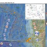
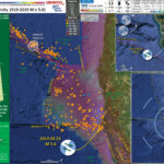
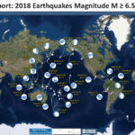
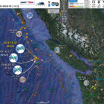
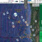
Initial Narrative

Well, it has been a very busy week. I had gotten back from the American Geophysical Union Fall Meeting in Chicago late Saturday night. I had one day to hang out with my cats before I was to head down to Santa Cruz to meet with the city there to discuss installing a tide gage. Santa Cruz lacks a gage yet receives large tsunami inundations.

So, I drove down and got there about 10pm Monday evening. I was up for an hour or two and went to sleep.

At shortly after 2:30am I got a text message about a M 6.4 earthquake near Ferndale. I immediately got up and texted my colleague Cynthia Pridmore. We are tasked to prepare Earthquake Quick Reports that we (California Geological Survey, CGS) provide to the California Governor’s Office of Emergency Services (Cal OES). These reports provide technical information that helps them provide resources to local first responders during times following natural hazards impacts.

https://earthquake.usgs.gov/earthquakes/eventpage/nc73821036/executive

These reports are reviewed by the head of the Seismic Hazards Program (Tim Dawson) and by the State Geologist prior to being provided to the leadership in our organization and parent organizations. Reports for larger earthquakes and tsunami sometimes end up on the Governor’s desk.

We got our report submitted within about 45 minutes and we prepared for a long couple of days. We at CGS met at 8am to discuss our field response activities.

CGS and the U.S. Geological Survey (USGS) work closely together to document field evidence from earthquakes and tsunami. Kate Thomas (CGS) and Luke Blair (USGS) have a database ready to go within about 15 minutes after an earthquake. This database is used on mobile devices to collect observational information that include photos and other information. We use the ESRI Field Maps app for this purpose.

We decided to send CGS staff from the Eureka office out to collect information. I was to drive back to Humboldt and then join the field teams the following day.

Something that also happens following significant or damaging earthquakes is the activation of the California Earthquake Clearinghouse. Pridmore (CGS) is the chair of the EQCH and works with our partners (USGS, EERI, etc.) to decide when to activate the EQCH.

Data from these CGS/USGS field observations, along with data from other field teams, are posted onto the EQCH page for this event. Here is where those data are made available for this M 6.4 Ferndale Earthquake. The dataset of field observations are posted on that page are found by clicking on the “Resources” tab, also linked here.

When I returned to my home, the power was still out. We (CGS) had a scheduled meeting at 6pm and the EQCH meeting at 7pm. So, I went to the Eureka National Weather Service (NWS) Office on Woodley Island. They have electric power backup and satellite internet access. I work closely with the NWS and Cal OES and have been granted access to set up my workstation there during natural hazard emergencies like earthquake and tsunami. This was we can all better coordinate our actions without the burden of having power or internet outages at our residences. We are thankful for these relationships between CGS, the NWS (Ryan Aylward, Troy Nicolini) and Cal OES Eureka (Todd Becker).

So, I got up very early to work with my co-workers to continue the field investigations. There was little geological evidence from the earthquake. We identified some landslides and cracks in road fill. We did not locate any evidence for liquefaction, even though the USGS liquefaction susceptibility data suggested a high chance for that phenomena.

The Earthquake Report

This earthquake is in a tectonically complicated region of the western United States, the Mendocino triple junction. Here, three plate boundary fault systems meet (the definition of a triple junction): the San Andreas fault from the south, the Cascadia subduction zone from the north, and the Mendocino fault from the west. These plate boundary fault systems all overlap like fingers do when we fold our hands together.

The Cascadia subduction zone is a convergent (moving together) plate boundary where the Gorda and Juan de Fuca plates dive into the Earth beneath the North America plate. The fault formed here is called the megathrust subduction zone fault. Earthquakes on subduction zone faults generate the largest magnitude earthquakes of all fault types and also generate tsunami that can impact the local area and also travel across the ocean to impact places elsewhere. The most recent known Cascadia megathrust subduction zone fault earthquake was in January 1700.

The San Andreas and Mendocino fault systems are strike-slip (plates move side by side) fault systems. Many are familiar with the 1906 San Francisco Earthquake.

While the largest source of annual seismicity are intraplate Gorda plate earthquakes, the two largest contributors to seismic hazards in California are the Cascadia subduction zone (CSZ) and the San Andreas fault (SAF) systems. These sources overlap in the region of the Mendocino triple junction (MTJ) and may interact in ways we are only beginning to understand as evidenced by the 2016 M7.8 Kaikōura earthquake in New Zealand (Clark et al., 2017 Litchfield et al., 2018), which occurred along a similar subduction/transform boundary, and included co-seismic rupture of more than 20 faults.

The M 6.4 earthquake was a strike-slip earthquake within the downgoing Gorda plate (an intra plate earthquake). The earthquake started offshore and then the fault slipped to the east.

There is modest evidence that this earthquake generated focused seismic waves in the direction of fault slip (this is called directivity). In addition, the area of the lower Eel River Valley is a sedimentary basin. Sedimentary basins are known for amplifying ground shaking and trapping seismic waves, further increasing the ground shaking. The lower Eel River Valley is formed by tectonic folding caused by the northward migration of the Mendocino triple junction (read my contributions in the 2022 Pacific Cell Friends of the Pleistocene guidebook for more information about the structure of the Eel River and Van Duzen River valleys and surrounding regions.

So the seismic waves could have been trapped in the sedimentary basin formed within the Eel River Valley. However, there is an even older sedimentary basin here in which the Eel/Van Duzen river sediments are deposited within. These older sedimentary rocks have different seismic velocity properties that could also affect how seismic waves are transmitted here. There is a terrane bounding fault that separates these older rocks (Cretaceous Franciscan Formation) to the south from the younger rocks (Quaternary-Tertiary Wildcat Group) to the north.

Also, any of the large crustal fault systems (e.g., the Russ fault, the Little Salmon or Table Bluff faults, etc.) could guide seismic waves (a.k.a. act as wave guides), directing them in orientations relative to the fault systems.

My leading hypothesis is that the younger (latest Pleistocene to Holocene) river sediments that form the younger sedimentary basin and the crustal faults are both responsible for modifying the seismic wave transmission from this earthquake.

One thing people almost always ask is about whether or not there is a higher chance that there will be a Cascadia subduction zone earthquake. This is currently impossible to tell. However, we can make some estimates of how forces within the Earth might have changed after a given earthquake. There was a Gorda plate earthquake sequence in 2018 that allowed us to consider these changes in the crust to see if the megathrust was brought more close to rupture. Here is the report from that Gorda plate earthquake sequence.

I will update this report further in the future, as we collect additional information.

One last thing for now. Bob McPherson formed a research group that we call Team Gorda. Team Gorda, supported by Connie Stewart at Cal Poly Humboldt, is using recently constructed fiber cables as a seismic instrument (called distributed acoustic seismic, DAS) to learn more about the underlying tectonic structures in the region. This fiber cable acts as thousands of little seismometers. Jeff McGuire and his team just installed the interrogator in our office at the Arcata City Hall. Horst from the Berkeley Seismic Lab is also working with Bob to install seismometers along the fiber cable so that we can calibrate the DAS observations.

We ran our first DAS experiment earlier this year and plan on doing more experiments far into the future, including fiber cables that are installed from here into the Pacific Ocean (on their way to Asia).

Below is my interpretive poster for this earthquake

  • I plot the seismicity from the past month, with diameter representing magnitude (see legend). I include earthquake epicenters from 1922-2022 with magnitudes M ≥ 3.0 in one version.
  • I plot the USGS fault plane solutions (moment tensors in blue and focal mechanisms in orange), possibly in addition to some relevant historic earthquakes.
  • A review of the basic base map variations and data that I use for the interpretive posters can be found on the Earthquake Reports page. I have improved these posters over time and some of this background information applies to the older posters.
  • Some basic fundamentals of earthquake geology and plate tectonics can be found on the Earthquake Plate Tectonic Fundamentals page.

    I include some inset figures. Some of the same figures are located in different places on the larger scale map below.

  • In the upper left corner is a map showing the western US and a century of seismicity.
  • In the upper right corner is a map that displays a variety of earthquake intensity information. I plot the USGS modeled intensity, the USGS Did You Feel It? observations of intensity, and the shaking magnitude using the Peak Ground Acceleration scale in units of g (gravitational acceleration). I describe this map later in the report.
  • To the left of the intensity map are two maps that show the probability (the chance of) earthquake triggered landslides and the susceptibility (the chance of) earthquake induced liquefaction. I will discuss these ground failure models later in the report.
  • In the lower right corner I include a plot of aftershocks from a three day period.
  • Here is the map with 3 month’s seismicity plotted.

  • Here is an updated interpretive poster with 3 day’s seismicity plotted. I describe how this poster is different
  • In the lower right corner is a map from the USGS. This map shows where they interpret the location for the causative fault for this earthquake. There are also arrows (vectors) that show how Global Navigation Satellite System (GNSS, used to be called GPS) sites moved during the earthquake and how the moved using a computer simulation of the Earth that incorporate a fault that slipped like shown on the map. These arrows show the direction of motion and the amount of motion.
  • To the left of this map is the USGS finite fault model for this earthquake. The colors represent the amount that the fault slipped during the earthquake. This is the fault model that they used to estimate how the GNSS sites moved in the map to the right.
  • In the upper right corner is a map that shows the seismicty from the past week (in orange) and seismicity associated with the earthquake sequence from exactly one year before (in blue).
  • In the main part of the map I plot the earthquake mechanisms from the past century.

    Seismicity Profile

  • I felt the M 4.1 earthquake this morning (24 Dec 2022). It was an extensional earthquake in the eastern part of the aftershock region.
  • Today I plotted the seismicity along an east-west profile.
  • I traced the Gorda plate geometry from Guo et al. (2018). This is from their profile B-B’ which is just about at 41 degrees north.
  • We can see that the mainshock (the M 6.4) and most of the aftershocks are within the Gorda plate.

  • Here is an updated plot that includes the USGS Finite Fault Model as a transparent overlay.
  • Note how most of the slip is in the North America plate.

  • Here is an updated plot that displays M 6.4 in blue and M 5.4 in green.

  • And if someone wants to learn more about what a hypocenter is, here you go >>>

    Aftershock Patterns

  • Yesterday I got to feel one of the aftershocks, an M 4.2 to the southeast of the main sequence.
  • Today I plotted all the aftershocks to date as of this morning. It appears that there were two main faults involved. One about 45 km long and another one about 25 km long.
  • I include earthquake mechanisms for all events that I could download today. I placed some mechanisms that may not be related to these 2 faults at 50% transparency.
  • This poster below includes a map (lower right corner) of the Cascadia subduction zone and the cross section showing how the crust deforms between (interseismic) and during (coseismic) earthquakes.
  • I also include a schematic showing where earthquakes might happen (upper left center). Earthquakes along the megathrust subduction zone fault are called interplate earthquakes (like the interstate highways connect between states).
  • Earthquakes within the Gorda or North America plates are called intraplate earthquakes. The M 6.4 was an intraplate earthquake within the Gorda plate. I don’t really have a good way to show intraplate strike-slip faults in this diagram (room for future work!).
  • In the upper right corner is the seismicity profile that I also show above in the report. When comparing the seismicity with the Guo et al. (2021) slab model, it appears that most of the earthquakes are within the Gorda crust. There are some above, possibly in the North America crust.

  • Here is another updated map, updated on 2 January 2023 to include the M 5.4 related earthquakes.
  • Now it appears that there are three main faults involved, at least.

  • Yesterday I was chatting with Bob McPherson as we were looking at the USGS finite fault slip model. Bob suggested that this model shows that the earthquake slipped in the Gorda and North America plates. If the slip model is correct, then Bob is correct. This is quite interesting if true.
  • UPDATE comment (4 jan ’23): I have seen other slip models that do not place M 6.4 slip above the Gorda plate. We must remember that these slip models are non unique solutions and that there is quite a bit of wiggle room for their solutions. Basically, there are knobs to turn on these models (allowing one to change parameters, such as the material properties of the Earth (e.g., the “rheology” of the crust or mantle)) and changing these parameters can change the results while still keeping a good fit to the observational data. It is not uncommon that the slip models for both nodal planes (the two possible fault planes shown on earthquake mechanisms (focal mechanisms or moment tensors)) each fit the data equally well. I have seen the fault model that was fit to the incorrect (incorrect relative to aftershocks) fault plane being chosen as the preferred slip model. So, we must remember this when we are interpreting model results like these fault slip models.
  • First lets just look at the finite fault slip model. Below we see a plot with color representing how much the fault slipped. The white star is the M 6.4 hypocenter (the 3-D location of the M 6.4). East is to the left and west is to the left (pretend you are looking at the diagram from the north side of the fault).
  • There are gray lines that represent times (10 seconds and 20 seconds after the M 6.4 mainshock) where the rupture propagation front was. So, the fault started slipping at the white star. Then, the fault moved and the outer limit of this motion radiated outwards and was at the first gray line in 10 seconds and at the second gray line at 20 seconds.
  • There are small gray arrows that show the direction and magnitude of slip motion along the fault. If we combine this plot with our knowledge that this was a left-lateral strike-slip earthquake, and we are looking to the south at the fault, we can surmise that these vectors are on the north side of the fault. Also, that the fault slipped from east of the hypocenter towards the hypocenter, and updip (shallower).

  • Yes, this would be quite interesting, if the fault broke both Gorda and North America crust. This would make our interpretation of the Mendocino triple junction even more complicated. There are not currently any faults mapped in the North America plate that align with this M 6.4 sequence.
  • It is possible that there are faults there, or that they may be blind (not reach the ground surface). If these faults are young, they may not have sufficient offset to produce deformation at the Earth’s surface.
  • We do have examples of this elsewhere, where there are crustal faults in the downgoing plate that are also in the same location but in the upper plate.
  • For example, Goldfinger et al. (1997) mapped a series of faults that cut across strike to the Cascadia subduction zone fault. Two, the Daisy Bank and Wecoma faults, are shown in their figure below. Note how these faults are mapped in the Juan de Fuca plate and propagate upwards into the accretionary prism (let’s call this the upper plate).

  • Block rotation model for the central Cascadia forearc. SeaBeam bathymetry shaded from the north. The Wecoma and Daisy Bank faults are show, with the Daisy Bank fault exposed in the foreground. Well-mapped fault traces are in solid; discontinuous traces are dashed. The arc-parallel component of oblique subduction creates a dextral share couple, which is accommodated by WNW trending left-lateral strike-slip faults. We propose that shearing of the slab due to oblique subduction is responsible for the fault involving oceanic crust. WF, Wecoma fault; DBF, Daisy bank fault; FF, Fulmar fault, “pr,” pressure ridge; “DB,” Daisy Bank; “OT?,” possible old left-lateral fault strand. Arrow heads and tails show strike-slip motion. White arrows at western end of Wecoma fault show eastward increasing slip calculated from isopach offsets.

  • Another place where I have seen this is offshore of Sumatra. When we were coring there for my Ph.D. research, we identified a strike-slip fault in the India Australia plate that propagated upwards into the accretionary prism (the “upper plate”).
  • One thing That this almost certainly requires is that the megathrust fault be seismogenically coupled in this area.
  • Basically, we need a mechanism by which, when the lower plate fault slips, that the forces are exerted to the upper plate to move in the same direction and manner as that observed in the lower plate. Having a coupled megathrust fault is one way to do this
  • And we have several examples of this in the southern CSZ. There are a number of strike-slip fault earthquakes within the Gorda plate (or along the Mendocino fault) offshore of the megathrust that generated differential motion for geodetic sites (like GNSS or GPS stations) during the earthquake.
  • Further down in the report I present the map from Dengler et al. (1994) that shows how geodetic sites in North America plate move in response to the 1994 Cape Mendocino fault right-lateral strike-slip earthquake.
  • The USGS pages for the GNSS network provide static offsets for the GNSS stations as observed for these Gorda plate earthquakes. Williams and McPherson (2006) present another example of this. Below we can see the coseismic displacements from the 2005 northeast striking left-lateral strike-slip fault earthquake.

  • Coseismic displacements from the 15-Jun-2005 M7.2 Gorda plate earthquake located (off the map) 156 km (97 miles) W (280°) from Trinidad, CA and 157 km (98 miles) WSW (251°) from Crescent City, CA. Note the similarity to the deformation pattern of the 1994 event. Continuously operating GPS stations shown here are operated and maintained through the Plate Boundary Observatory component (pboweb.unavco. org) of the National Science Foundation’s EarthScope project
    (www.earthscope.org).

  • Regardless of whether or not there is a throughgoing fault, it is clear that the megathrust fault is locked here. (either from the presence of a throughoing fault or from the static offsets at these GNSS sites.
  • Below is the USGS finite fault slip model and a comparison between the observed GNSS offsets and the offsets modeled by placing slip on the finite fault model in an elastic half space.
  • Once we have better INSAR data (presuming these data will exist), this slip model may improve.

  • Mapped Geology

  • Here is a map that shows the mapped geologic units. Some of the map is from McLaughlin et al. (2000) and some is from the California Division of Mines and Geology (CDMG, 1999) which is now the California Geological Survey.
  • There are about 30 units in each dataset, so I chose to simply use their labels from the respective databases. The CDMG labels are basically the same as the geologic unit (e.g., Franciscan is something like TKJf) while McLaughlin mapped units relative to their geomorphic expression, so units have strange labels (e.g., Franciscan is something like co1 or cm1).
  • Note that the seismicity trend from the M 6.4 does not align with the faults nor the geologic units in the North America plate. This makes the linkage between rupturing in the Gorda and the North America plates more tenuous (though still possible).

    Earlier Report Interpretive Posters

  • Here is the poster from last year’s earthquake sequence.

  • Here are two relevant interpretive posters from the 1992 Cape Mendocino Earthquake.
  • This one is an overview of the earthquake.

  • This one helps us compare the mainshock and two main triggered earthquakes.

  • Here is a poster that shows a comparison between the 1991 Honeydew and 1992 Cape Mendocino earthquakes..

    Some Relevant Discussion and Figures

    • Here is a map of the Cascadia subduction zone, modified from Nelson et al. (2006). The Juan de Fuca and Gorda plates subduct norteastwardly beneath the North America plate at rates ranging from 29- to 45-mm/yr. Sites where evidence of past earthquakes (paleoseismology) are denoted by white dots. Where there is also evidence for past CSZ tsunami, there are black dots. These paleoseismology sites are labeled (e.g. Humboldt Bay). Some submarine paleoseismology core sites are also shown as grey dots. The two main spreading ridges are not labeled, but the northern one is the Juan de Fuca ridge (where oceanic crust is formed for the Juan de Fuca plate) and the southern one is the Gorda rise (where the oceanic crust is formed for the Gorda plate).

    • Here is a version of the CSZ cross section alone (Plafker, 1972). This shows two parts of the earthquake cycle: the interseismic part (between earthquakes) and the coseismic part (during earthquakes). Regions that experience uplift during the interseismic period tend to experience subsidence during the coseismic period.

    • This figure shows how a subduction zone deforms between (interseismic) and during (coseismic) earthquakes. We also can see how a subduction zone generates a tsunami. Atwater et al., 2005.

    • Here is an animation produced by the folks at Cal Tech following the 2004 Sumatra-Andaman subduction zone earthquake. I have several posts about that earthquake here and here. One may learn more about this animation, as well as download this animation here.

    The Gorda and Juan de Fuca plates subduct beneath the North America plate to form the Cascadia subduction zone fault system. In 1992 there was a swarm of earthquakes with the magnitude Mw 7.2 Mainshock on 4/25. Initially this earthquake was interpreted to have been on the Cascadia subduction zone (CSZ). The moment tensor shows a compressional mechanism. However the two largest aftershocks on 4/26/1992 (Mw 6.5 and Mw 6.7), had strike-slip moment tensors. In my mind, these two aftershocks aligned on what may be the eastern extension of the Mendocino fault. However, looking at their locations, my mind was incorrect. These two earthquakes were not aftershocks, but were either left-lateral or right-lateral strike-slip Gorda plate earthquakes triggered by the M 7.1 thrust event.

    These two quakes appear to be aligned with the two northwest trends in seismicity and the 18 March 2020 M 5.2. The orientation of the mechanisms are not as perfectly well aligned, but there are lots of reasons for this (perhaps the faults were formed in a slightly different orientation, but have rotated slightly).

    There have been several series of intra-plate earthquakes in the Gorda plate. Two main shocks that I plot of this type of earthquake are the 1980 (Mw 7.2) and 2005 (Mw 7.2) earthquakes. I place orange lines approximately where the faults are that ruptured in 1980 and 2005. These are also plotted in the Rollins and Stein (2010) figure above. The Gorda plate is being deformed due to compression between the Pacific plate to the south and the Juan de Fuca plate to the north. Due to this north-south compression, the plate is deforming internally so that normal faults that formed at the spreading center (the Gorda Rise) are reactivated as left-lateral strike-slip faults. In 2014, there was another swarm of left-lateral earthquakes in the Gorda plate. I posted some material about the Gorda plate setting on this page.

    • This is the map used in the animation below. Earthquake epicenters are plotted (some with USGS moment tensors) for this region from 1917-2017 with M ≥ 6.5. I labeled the plates and shaded their general location in different colors.
    • I include some inset maps.
      • In the upper right corner is a map of the Cascadia subduction zone (Chaytor et al., 2004; Nelson et al., 2004).
      • In the upper left corner is a map from Rollins and Stein (2010). They plot epicenters and fault lines involved in earthquakes between 1976 and 2010.


    • Here is a map from Rollins and Stein, showing their interpretations of different historic earthquakes in the region. This was published in response to the Januray 2010 Gorda plate earthquake. The faults are from Chaytor et al. (2004).

    • Tectonic configuration of the Gorda deformation zone and locations and source models for 1976–2010 M ≥ 5.9 earthquakes. Letters designate chronological order of earthquakes (Table 1 and Appendix A). Plate motion vectors relative to the Pacific Plate (gray arrows in main diagram) are from Wilson [1989], with Cande and Kent’s [1995] timescale correction.

    • Here is a large scale map of the 1994 earthquake swarm. The mainshock epicenter is a black star and epicenters are denoted as white circles.

    • Here is a plot of focal mechanisms from the Dengler et al. (1995) paper in California Geology.

  • In this map below, I label a number of other significant earthquakes in this Mendocino triple junction region. Another historic right-lateral earthquake on the Mendocino fault system was in 1994. There was a series of earthquakes possibly along the easternmost section of the Mendocino fault system in late January 2015, here is my post about that earthquake series.

  • Here is a map from Chaytor et al. (2004) that shows some details of the faulting in the region. The moment tensor (at the moment i write this) shows a north-south striking fault with a reverse or thrust faulting mechanism. While this region of faulting is dominated by strike slip faults (and most all prior earthquake moment tensors showed strike slip earthquakes), when strike slip faults bend, they can create compression (transpression) and extension (transtension). This transpressive or transtentional deformation may produce thrust/reverse earthquakes or normal fault earthquakes, respectively. The transverse ranges north of Los Angeles are an example of uplift/transpression due to the bend in the San Andreas fault in that region.

  • A: Mapped faults and fault-related ridges within Gorda plate based on basement structure and surface morphology, overlain on bathymetric contours (gray lines—250 m interval). Approximate boundaries of three structural segments are also shown. Black arrows indicated approximate location of possible northwest- trending large-scale folds. B, C: uninterpreted and interpreted enlargements of center of plate showing location of interpreted second-generation strike-slip faults and features that they appear to offset. OSC—overlapping spreading center.

  • These are the models for tectonic deformation within the Gorda plate as presented by Jason Chaytor in 2004.
  • Mw = 5 Trinidad Chaytor

    Models of brittle deformation for Gorda plate overlain on magnetic anomalies modified from Raff and Mason (1961). Models A–F were proposed prior to collection and analysis of full-plate multibeam data. Deformation model of Gulick et al. (2001) is included in model A. Model G represents modification of Stoddard’s (1987) flexural-slip model proposed in this paper.

Mendocino triple junction video

Shaking Intensity

  • Here is a figure that shows a more detailed comparison between the modeled intensity and the reported intensity. Both data use the same color scale, the Modified Mercalli Intensity Scale (MMI). More about this can be found here. The colors and contours on the map are results from the USGS modeled intensity. The DYFI data are plotted as colored dots (color = MMI, diameter = number of reports).
  • In the upper panel is the USGS Did You Feel It reports map, showing reports as colored dots using the MMI color scale. Underlain on this map are colored areas showing the USGS modeled estimate for shaking intensity (MMI scale).
  • I also plot, in colored squares, the ground motions recorded on seismometers operated by the CGS Strong Motion Instrument Program (SMIP), run by Hamid Haddadi. Units are relative to gravitation acceleration where 1 = 1g. g is defined as the acceleration at the Earth’s surface (9.8 m/s^2). Here is the data page for this M 6.4 earthquake. The largest acceleration (1.36g) is from a seismometer attached to a bridge and seismologists think that this large acceleration is due to the bridge in some way. Here is the SMIP data page for the M 5.4 earthquake.
  • Below the upper map plot is the USGS MMI Intensity scale, which lists the level of damage for each level of intensity, along with approximate measures of how strongly the ground shakes at these intensities, showing levels in acceleration (Peak Ground Acceleration, PGA) and velocity (Peak Ground Velocity, PGV).
  • In the lower panel is a plot showing MMI intensity (vertical axis) relative to distance from the earthquake (horizontal axis). The models are represented by the green and orange lines. The DYFI data are plotted as light blue dots. The mean and median (different types of “average”) are plotted as orange and purple dots. Note how well (or poorly) the reports fit the brown line (the model that represents how MMI works based on quakes in California). The increased intensity on the left of the plot (which are closer to the earthquake) are the records that show intensities higher than expected from the modeling.

  • Here is an animation from the USGS and Cal Tech that shows a simulation of seismic waves from this M 6.4 earthquake.
  • There is a link to this video from the earthquake page.

Shaking Intensity and Potential for Ground Failure

  • Below are a series of maps that show the shaking intensity and potential for landslides and liquefaction. These are all USGS data products.
  • There are many different ways in which a landslide can be triggered. The first order relations behind slope failure (landslides) is that the “resisting” forces that are preventing slope failure (e.g. the strength of the bedrock or soil) are overcome by the “driving” forces that are pushing this land downwards (e.g. gravity). The ratio of resisting forces to driving forces is called the Factor of Safety (FOS). We can write this ratio like this:

    FOS = Resisting Force / Driving Force

    When FOS > 1, the slope is stable and when FOS < 1, the slope fails and we get a landslide. The illustration below shows these relations. Note how the slope angle α can take part in this ratio (the steeper the slope, the greater impact of the mass of the slope can contribute to driving forces). The real world is more complicated than the simplified illustration below.


    Landslide ground shaking can change the Factor of Safety in several ways that might increase the driving force or decrease the resisting force. Keefer (1984) studied a global data set of earthquake triggered landslides and found that larger earthquakes trigger larger and more numerous landslides across a larger area than do smaller earthquakes. Earthquakes can cause landslides because the seismic waves can cause the driving force to increase (the earthquake motions can “push” the land downwards), leading to a landslide. In addition, ground shaking can change the strength of these earth materials (a form of resisting force) with a process called liquefaction.

    Sediment or soil strength is based upon the ability for sediment particles to push against each other without moving. This is a combination of friction and the forces exerted between these particles. This is loosely what we call the “angle of internal friction.” Liquefaction is a process by which pore pressure increases cause water to push out against the sediment particles so that they are no longer touching.

    An analogy that some may be familiar with relates to a visit to the beach. When one is walking on the wet sand near the shoreline, the sand may hold the weight of our body generally pretty well. However, if we stop and vibrate our feet back and forth, this causes pore pressure to increase and we sink into the sand as the sand liquefies. Or, at least our feet sink into the sand.

    Below is a diagram showing how an increase in pore pressure can push against the sediment particles so that they are not touching any more. This allows the particles to move around and this is why our feet sink in the sand in the analogy above. This is also what changes the strength of earth materials such that a landslide can be triggered.


    Below is a diagram based upon a publication designed to educate the public about landslides and the processes that trigger them (USGS, 2004). Additional background information about landslide types can be found in Highland et al. (2008). There was a variety of landslide types that can be observed surrounding the earthquake region. So, this illustration can help people when they observing the landscape response to the earthquake whether they are using aerial imagery, photos in newspaper or website articles, or videos on social media. Will you be able to locate a landslide scarp or the toe of a landslide? This figure shows a rotational landslide, one where the land rotates along a curvilinear failure surface.


  • Below is the liquefaction susceptibility and landslide probability map (Jessee et al., 2017; Zhu et al., 2017). Please head over to that report for more information about the USGS Ground Failure products (landslides and liquefaction). Basically, earthquakes shake the ground and this ground shaking can cause landslides. We can see that there is a low probability for landslides. However, we have already seen photographic evidence for landslides and the lower limit for earthquake triggered landslides is magnitude M 5.5 (from Keefer 1984)
  • I use the same color scheme that the USGS uses on their website. Note how the areas that are more likely to have experienced earthquake induced liquefaction are in the valleys. Learn more about how the USGS prepares these model results here.

Seismic Hazard and Seismic Risk

  • These are two maps from the Global Earthquake Model (GEM) project, the GEM Seismic Hazard and the GEM Seismic Risk maps from Pagani et al. (2018) and Silva et al. (2018).
  • The GEM Seismic Hazard Map:


  • The Global Earthquake Model (GEM) Global Seismic Hazard Map (version 2018.1) depicts the geographic distribution of the Peak Ground Acceleration (PGA) with a 10% probability of being exceeded in 50 years, computed for reference rock conditions (shear wave velocity, VS30, of 760-800 m/s). The map was created by collating maps computed using national and regional probabilistic seismic hazard models developed by various institutions and projects, and by GEM Foundation scientists. The OpenQuake engine, an open-source seismic hazard and risk calculation software developed principally by the GEM Foundation, was used to calculate the hazard values. A smoothing methodology was applied to homogenise hazard values along the model borders. The map is based on a database of hazard models described using the OpenQuake engine data format (NRML). Due to possible model limitations, regions portrayed with low hazard may still experience potentially damaging earthquakes.
  • Here is a view of the GEM seismic hazard map for the USA.

  • The GEM Seismic Risk Map:


  • The Global Seismic Risk Map (v2018.1) presents the geographic distribution of average annual loss (USD) normalised by the average construction costs of the respective country (USD/m2) due to ground shaking in the residential, commercial and industrial building stock, considering contents, structural and non-structural components. The normalised metric allows a direct comparison of the risk between countries with widely different construction costs. It does not consider the effects of tsunamis, liquefaction, landslides, and fires following earthquakes. The loss estimates are from direct physical damage to buildings due to shaking, and thus damage to infrastructure or indirect losses due to business interruption are not included. The average annual losses are presented on a hexagonal grid, with a spacing of 0.30 x 0.34 decimal degrees (approximately 1,000 km2 at the equator). The average annual losses were computed using the event-based calculator of the OpenQuake engine, an open-source software for seismic hazard and risk analysis developed by the GEM Foundation. The seismic hazard, exposure and vulnerability models employed in these calculations were provided by national institutions, or developed within the scope of regional programs or bilateral collaborations.
  • Here is a view of the GEM seismic risk map for the USA. Note how the seismic risk is higher in places of larger population (like Los Angeles and San Francisco).

Stress Triggering

  • When an earthquake fault slips, the crust surrounding the fault squishes and expands, deforming elastically (like in one’s underwear). These changes in shape of the crust cause earthquake fault stresses to change. These changes in stress can either increase or decrease the chance of another earthquake.
  • I wrote more about this type of earthquake triggering for Temblor here. Head over there to learn more about “static coulomb stress triggering.”
  • Rollins and Stein (2010) conducted this type of analysis for the 2010 M 6.5 Gorda Earthquake. They found that some of the faults in the region experienced an increase in fault stress (the red areas on the figure below). These changes in stress are very small, so require a fault to be at the “tipping point” for these changes in stress to cause an earthquake.
  • There was a triggered earthquake in this sequence. There was a M 5.9 event about 25 days after the mainshock, this earthquake happened in a region that saw increased stress after the M 6.5. The M 5.9 appears to have been on the same fault as the M 6.5
  • First, here is the fault model that Rollins and Stein used in their analysis of stress changes from the 2010 earthquake.

  • Source models for earthquakes S and T, 10 January 2010, M = 6.5, and 4 February 2010, Mw = 5.9.

  • Let’s take a look at some examples of analogic earthquakes to the 2010 temblor. First, here is a plot showing changes in stress following the 1980 Trinidad Earthquake (a very damaging earthquake in the region). This is the largest historic earthquake in the region at magnitude M 7.3 (other than the 1906 San Francisco Earthquake).

  • Coulomb stress changes imparted by the 1980 Mw = 7.3 earthquake (B) to a matrix of faults representing the Mendocino Fault Zone, the Cascadia subduction zone, and NE striking left‐lateral faults in the Gorda zone. The Mendocino Fault Zone is represented by right‐lateral faults whose strike rotates from 285° in the east to 270° in the west; Cascadia is represented by reverse faults striking 350° and dipping 9°; faults in the Gorda zone are represented by vertical left‐lateral faults striking 45°. The boundary between the left‐lateral “zone” and the reverse “zone” in the fault matrix is placed at the 6 km depth contour on Cascadia, approximated by extending the top edge of the Oppenheimer et al.
    [1993] model for the 1992 Cape Mendocino earthquake (J). Calculation depth is 5 km. The numbered brackets are groups of aftershocks from Hill et al. [1990].

  • Next let’s look at the stress changes following the 2005 M 7.2 earthquake.

  • Coulomb stress changes imparted by the Shao and Ji (2005) variable slip model for the 15 June 2005 Mw = 7.2 earthquake (P) to the epicenter of the 17 June 2005 Mw = 6.6 earthquake (Q). Calculation depth is 10 km.

  • Here is the figure we have all been waiting for (actually, the next one is cool too). This figure shows the changes in stress associated with the 2010 M 6.5 earthquake. Remember, these are just models.

  • Coulomb stress changes imparted by the D. Dreger (unpublished report, 2010, [no longer] available at http://seismo.berkeley.edu/∼dreger/jan10210_ff_summary.pdf) model for the January 2010 M = 6.5 shock (S) to nearby faults. East of the dashed line, stress changes are resolved on the Cascadia subduction zone, represented by a northward extension of the Oppenheimer et al. [1993] rupture plane for the 1992 Mw = 6.9 Cape Mendocino earthquake. West of the dashed line, stress changes are resolved on the NW striking nodal plane for the February 2010 Mw = 5.9 earthquake (T) at a depth of 23.6 km.

  • This is the main take-away figure from Rollins and Stein (2010). For each map, there is a source fault (in black) and receiver faults (red or blue, depending on the change in stress).
  • For example, in a, the source is a gorda plate left-lateral strike-slip fault. Parts of the Cascadia megathrust are represented on the right (triangles, labeled thrust). They also model changes in stress on the Mendocino fault (the red and blue lines at the bottom of “a”).

  • And, you thought it couldn’t get any better. Here is yet another fantastic figure showing the stress change on the Cascadia megathrust fault and on the Mendocino fault following the 2010 M 6.5 earthquake.

    References:

    Basic & General References

  • Frisch, W., Meschede, M., Blakey, R., 2011. Plate Tectonics, Springer-Verlag, London, 213 pp.
  • Hayes, G., 2018, Slab2 – A Comprehensive Subduction Zone Geometry Model: U.S. Geological Survey data release, https://doi.org/10.5066/F7PV6JNV.
  • Holt, W. E., C. Kreemer, A. J. Haines, L. Estey, C. Meertens, G. Blewitt, and D. Lavallee (2005), Project helps constrain continental dynamics and seismic hazards, Eos Trans. AGU, 86(41), 383–387, , https://doi.org/10.1029/2005EO410002. /li>
  • Jessee, M.A.N., Hamburger, M. W., Allstadt, K., Wald, D. J., Robeson, S. M., Tanyas, H., et al. (2018). A global empirical model for near-real-time assessment of seismically induced landslides. Journal of Geophysical Research: Earth Surface, 123, 1835–1859. https://doi.org/10.1029/2017JF004494
  • Kreemer, C., J. Haines, W. Holt, G. Blewitt, and D. Lavallee (2000), On the determination of a global strain rate model, Geophys. J. Int., 52(10), 765–770.
  • Kreemer, C., W. E. Holt, and A. J. Haines (2003), An integrated global model of present-day plate motions and plate boundary deformation, Geophys. J. Int., 154(1), 8–34, , https://doi.org/10.1046/j.1365-246X.2003.01917.x.
  • Kreemer, C., G. Blewitt, E.C. Klein, 2014. A geodetic plate motion and Global Strain Rate Model in Geochemistry, Geophysics, Geosystems, v. 15, p. 3849-3889, https://doi.org/10.1002/2014GC005407.
  • Meyer, B., Saltus, R., Chulliat, a., 2017. EMAG2: Earth Magnetic Anomaly Grid (2-arc-minute resolution) Version 3. National Centers for Environmental Information, NOAA. Model. https://doi.org/10.7289/V5H70CVX
  • Müller, R.D., Sdrolias, M., Gaina, C. and Roest, W.R., 2008, Age spreading rates and spreading asymmetry of the world’s ocean crust in Geochemistry, Geophysics, Geosystems, 9, Q04006, https://doi.org/10.1029/2007GC001743
  • Pagani, M., J. Garcia-Pelaez, R. Gee, K. Johnson, V. Poggi, R. Styron, G. Weatherill, M. Simionato, D. Viganò, L. Danciu, D. Monelli (2018). Global Earthquake Model (GEM) Seismic Hazard Map (version 2018.1 – December 2018), DOI: 10.13117/GEM-GLOBAL-SEISMIC-HAZARD-MAP-2018.1
  • Silva, V ., D Amo-Oduro, A Calderon, J Dabbeek, V Despotaki, L Martins, A Rao, M Simionato, D Viganò, C Yepes, A Acevedo, N Horspool, H Crowley, K Jaiswal, M Journeay, M Pittore, 2018. Global Earthquake Model (GEM) Seismic Risk Map (version 2018.1). https://doi.org/10.13117/GEM-GLOBAL-SEISMIC-RISK-MAP-2018.1
  • Zhu, J., Baise, L. G., Thompson, E. M., 2017, An Updated Geospatial Liquefaction Model for Global Application, Bulletin of the Seismological Society of America, 107, p 1365-1385, https://doi.org/0.1785/0120160198
  • Specific References

  • Atwater, B.F., Musumi-Rokkaku, S., Satake, K., Tsuju, Y., Eueda, K., and Yamaguchi, D.K., 2005. The Orphan Tsunami of 1700—Japanese Clues to a Parent Earthquake in North America, USGS Professional Paper 1707, USGS, Reston, VA, 144 pp.
  • Chaytor, J.D., Goldfinger, C., Dziak, R.P., and Fox, C.G., 2004. Active deformation of the Gorda plate: Constraining deformation models with new geophysical data: Geology v. 32, p. 353-356.
  • Dengler, L.A., Moley, K.M., McPherson, R.C., Pasyanos, M., Dewey, J.W., and Murray, M., 1995. The September 1, 1994 Mendocino Fault Earthquake, California Geology, Marc/April 1995, p. 43-53.
  • Geist, E.L. and Andrews D.J., 2000. Slip rates on San Francisco Bay area faults from anelastic deformation of the continental lithosphere, Journal of Geophysical Research, v. 105, no. B11, p. 25,543-25,552.
  • Guo, H., McGuire, J., and Zhang, H., 2021. Correlation of porosity variations and rheological transitions on the southern Cascadia megathrust in Nature Geoscience, https://doi.org/10.1038/s41561-021-00740-1
  • Irwin, W.P., 1990. Quaternary deformation, in Wallace, R.E. (ed.), 1990, The San Andreas Fault system, California: U.S. Geological Survey Professional Paper 1515, online at: http://pubs.usgs.gov/pp/1990/1515/
  • McCrory, P.A.,. Blair, J.L., Waldhauser, F., kand Oppenheimer, D.H., 2012. Juan de Fuca slab geometry and its relation to Wadati-Benioff zone seismicity in JGR, v. 117, B09306, doi:10.1029/2012JB009407.
  • McLaughlin, R.J., Ellen, S.D., Blake, M.C. Jr., Jayko, A.S., Irwin, W.P., Aalto, F.R., Carver, G.A., and Clarke, S.H. Jr., 2000. Geology of the Cape Mendocino, Eureka, Garberville, and Southwestern Part of the Hayfork 30 x 60 Minute Quadrangles and Adjacent Offshore Area, Northern California, USGS Miscellaneous Field Studies Map MF-2336, http://pubs.usgs.gov/mf/2000/2336/
  • McLaughlin, R.J., Sarna-Wojcicki, A.M., Wagner, D.L., Fleck, R.J., Langenheim, V.E., Jachens, R.C., Clahan, K., and Allen, J.R., 2012. Evolution of the Rodgers Creek–Maacama right-lateral fault system and associated basins east of the northward-migrating Mendocino Triple Junction, northern California in Geosphere, v. 8, no. 2., p. 342-373.
  • Nelson, A.R., Asquith, A.C., and Grant, W.C., 2004. Great Earthquakes and Tsunamis of the Past 2000 Years at the Salmon River Estuary, Central Oregon Coast, USA: Bulletin of the Seismological Society of America, Vol. 94, No. 4, pp. 1276–1292
  • Rollins, J.C. and Stein, R.S., 2010. Coulomb stress interactions among M ≥ 5.9 earthquakes in the Gorda deformation zone and on the Mendocino Fault Zone, Cascadia subduction zone, and northern San Andreas Fault: Journal of Geophysical Research, v. 115, B12306, doi:10.1029/2009JB007117, 2010.
  • Stoffer, P.W., 2006, Where’s the San Andreas Fault? A guidebook to tracing the fault on public lands in the San Francisco Bay region: U.S. Geological Survey General Interest Publication 16, 123 p., online at http://pubs.usgs.gov/gip/2006/16/
  • Wallace, Robert E., ed., 1990, The San Andreas fault system, California: U.S. Geological Survey Professional Paper 1515, 283 p. [http://pubs.usgs.gov/pp/1988/1434/].
  • Wells, D.L., and Coopersmith, K.J., 1994. New empirical relationships among magnitude, rupture length, rupture width, rupture area, and surface displacement in BSSA, v. 84, no. 4, p. 974-1002
  • Wells, R.E., Blakely, R.J., Wech, A.G., McCrory, P.A., Michael, A., 2017. Cascadia subduction tremor muted by crustal faults in Geology, v. 45, no. 6, p. 515–518, https://doi.org/10.1130/G38835.1
  • Williams, T.B. and McPherson, R.C., (2006). Gorda Plate Deformation Contributes to Shortening Between the Klamath Block and the On-land Portion of the Accretionary Prism to the S. Cascadia Subduction Zone. In Hemphill-Haley, M., McPherson, R., Patton, J. R., Stallman, J., Leroy, T.H., Sutherland, D., and Williams, T.B., eds. (2006) Pacific Cell Friends of the Pleistocene Field Trip Guidebook, The Triangle of Doom: Signatures of Quaternary Crustal Deformation in the Mendocino Deformation Zone (MDZ) Arcata, CA.

Return to the Earthquake Reports page.

Earthquake Report: Gorda Rise

It was a busy week (usual, right?). The previous week I was working on getting a house remodel done so someone could move in (they have been sleeping on couches for 6 months, so want to get them in asap). This week I spent lots of time putting final touches on a USGS National Earthquake Hazards Reduction Program external grant proposal together, proposing to conduct a paleoseismic investigation for a fault I discovered in late 2018 (see AGU poster here). So, I am catching up on my earthquake reporting for this earthquake offshore northern California.
On 18 May 2020 there was a magnitude M 5.5 extensional earthquake located near the Gorda Rise, an oceanic spreading ridge where oceanic crust is formed to create (love using the word create in science) the Gorda and Pacific plates.
https://earthquake.usgs.gov/earthquakes/eventpage/us70009jgy/executive
There are three types of plate boundaries and three types of earthquake faults (this is not a coincidence because plate boundaries are generally in the form of earthquake faults).

  1. Some plates move side-by-side to form transform plate boundaries (in the form of strike-slip faults, like the San Andreas fault).
  2. Some plates move towards each other to form convergent plate boundaries (in the form of subduction zone megathrust faults (like the Cascadia subduction zone), or collision zones(like the fault system that forms the uplift that created the Himalayas).
  3. Some plates move away from each other to form divergent plate boundaries (in the form of oceanic spreading ridges, or spreading centers, like the Mid Atlantic Ridge or the Gorda Rise; in these locations “normal” faults are formed).

More about different types of faults can be found here.
The northeast Pacific (aka Pacific Northwest as viewed by land lubbers) is dominated by the plate boundary formed between the Pacific (PP) and North America plates (NAP). In much of California, this plate boundary is realized in the form of the San Andreas fault (SAF), where the PP moves north relative to the NAP. Both plates are moving to the northwest, but the PP is moving faster, so it appears that the NAP is moving south. This southerly motion is relative not absolute. I present a background of the SAF in my review of the 1906 San Francisco earthquake here.
Near Cape Mendocino, in Humboldt County, California, the plate boundary gets more complicated and involves all three types of fault systems.
It appears that the San Andreas fault terminates in the King Range, causing some of the highest tectonic uplift rates in North America. There are sibling faults to the east of the San Andreas that continue further north (e.g. the Maacama fault turns into the Garberville fault and the Bartlett Springs fault (eventually) turns into the Bald Mountain/Big Lagoon fault. So, it looks like these San Andreas related faults extend offshore, possibly to at least the Oregon border. Geodetic evidence supports this, as first published by Williams et al. (2002).
The San Andreas ends near the beginning of the Cascadia subduction zone (CSZ), formed where the Gorda/Juan de Fuca/Explorer plates dive eastwards beneath the North America plate. More about the CSZ can be found here, where I describe the basis of our knowledge about prehistoric earthquakes and tsunami along the CSZ.
Far offshore of the CSZ are oceanic spreading ridges, the Gorda Rise and the Juan de Fuca Ridge. Because the plates are moving away from each other here (we think this is due to processes called slab pull and ridge push; slab pull describes the process that in the subduction zone, the downgoing oceanic plate is going deep into the mantle and pulling down the crust; ridge push is not really pushing from the ridge, but that there is additional mass added to the crust and this pushes down and then out, pushing the plate away from the ridge, towards the subduction zone). As these plates diverge, there is lowered pressure beneath this divergent zone. These lowered pressures cause the mantle to melt, leading to eruptions of mafic lava. When the lava cools, it becomes new oceanic crust.
Connecting the CSZ with these spreading ridges, and spreading ridges with other spreading ridges, are transform plate boundaries in the form of strike-slip faults. For example, the Mendocino fault and the Blanco fault. Here is a report that includes background information about the Mendocino fault. Here is a report with some background information about the Blamco fault.
The 18 May 2020 M 5.5 earthquake happened near the Gorda Rise and was an extensional earthquake. As the Gorda plate moves away from the spreading ridge, the normal faults formed at the ridge don’t disappear. The Gorda plate is a strange plate as it gets internally deformed, so as the plate moves towards the subduction zone, these normal faults get reactivated as strike-slip faults. These strike-slip faults have been responsible for some of the most damaging earthquakes to impact coastal northern California. More about these left-lateral strike-slip Gorda plate earthquakes can be found in a report here.
The M 5.5 earthquake happened along one of these normal faults, before that fault turns into a strike-slip fault. There is a good history of earthquakes just like this one. Here is a report for a similar event further to the north, also slightly east of the Gorda Rise.
One of the most common questions people have is, “does this earthquake change our chances for a CSZ earthquake?” The answer is no. The reason is because the stress changes from earthquakes extends for a limited distance from those earthquakes. I spend more time discussing this limitation for the Blanco fault here. Basically, this M 5.5 event was too small and too far away from the CSZ to change the chance that the CSZ will slip. Today is not different from a couple weeks ago: we always need to be ready for an earthquake when we live in earthquake country.

Below is my interpretive poster for this earthquake

  • I plot the seismicity from the past month, with diameter representing magnitude (see legend). I include earthquake epicenters from 1920-2020 with magnitudes M ≥ 5.0 in one version.
  • I plot the USGS fault plane solutions (moment tensors in blue and focal mechanisms in orange), possibly in addition to some relevant historic earthquakes.
  • A review of the basic base map variations and data that I use for the interpretive posters can be found on the Earthquake Reports page.
  • Some basic fundamentals of earthquake geology and plate tectonics can be found on the Earthquake Plate Tectonic Fundamentals page.

    I include some inset figures. Some of the same figures are located in different places on the larger scale map below.

  • In the upper right corner is a map and cross section for the Cascadia subduction zone. I spend more time describing these figures below.
  • In the upper left corner is a map showing this entire region with historic seismicity plotted. I also include the plate boundaries (USGS) and include the magnetic anomalies too. Read more about magnetic anomalies here. Notice how the magnetic anomaly bands are parallel to the spreading ridges. Why do you think this might be?
  • Yes, you are correct! The magnetic anomalies are parallel to the spreading ridges because they are formed when the crust cools along these spreading ridges.
  • The Gorda plate is being crushed between all the other plates in the area. This causes the plate to deform internally. The figure in the lower right corner (Chaytor et al., 2004) shows some different models to explain the faults formed from this internal deformation. The map in the upper right center, also from Chaytor et al. (2004) shows how they interpret some of these normal faults to be reactivated as strike-slip faults.
  • Here is the map with a month’s seismicity plotted.

  • Here are two posters from the 2018 Gorda Rise earthquakes.

  • This version includes earthquakes M ≥ 5.0 from the USGS. Note how the region where today’s earthquakes happened is a region of higher levels of seismicity. Perhaps this is because this region is the locus of the deformation within the Mendocino deformation zone?

Other Report Pages

Some Relevant Discussion and Figures

  • Here is a map of the Cascadia subduction zone, modified from Nelson et al. (2006). The Juan de Fuca and Gorda plates subduct norteastwardly beneath the North America plate at rates ranging from 29- to 45-mm/yr. Sites where evidence of past earthquakes (paleoseismology) are denoted by white dots. Where there is also evidence for past CSZ tsunami, there are black dots. These paleoseismology sites are labeled (e.g. Humboldt Bay). Some submarine paleoseismology core sites are also shown as grey dots. The two main spreading ridges are not labeled, but the northern one is the Juan de Fuca ridge (where oceanic crust is formed for the Juan de Fuca plate) and the southern one is the Gorda rise (where the oceanic crust is formed for the Gorda plate).

  • Here is a version of the CSZ cross section alone (Plafker, 1972). This shows two parts of the earthquake cycle: the interseismic part (between earthquakes) and the coseismic part (during earthquakes). Regions that experience uplift during the interseismic period tend to experience subsidence during the coseismic period.

  • This figure shows how a subduction zone deforms between (interseismic) and during (coseismic) earthquakes. We also can see how a subduction zone generates a tsunami. Atwater et al., 2005.

  • Here is an animation produced by the folks at Cal Tech following the 2004 Sumatra-Andaman subduction zone earthquake. I have several posts about that earthquake here and here. One may learn more about this animation, as well as download this animation here.
  • Here is a map from Chaytor et al. (2004) that shows some details of the faulting in the region. The moment tensor (at the moment i write this) shows a north-south striking fault with a reverse or thrust faulting mechanism. While this region of faulting is dominated by strike slip faults (and most all prior earthquake moment tensors showed strike slip earthquakes), when strike slip faults bend, they can create compression (transpression) and extension (transtension). This transpressive or transtentional deformation may produce thrust/reverse earthquakes or normal fault earthquakes, respectively. The transverse ranges north of Los Angeles are an example of uplift/transpression due to the bend in the San Andreas fault in that region.

  • A: Mapped faults and fault-related ridges within Gorda plate based on basement structure and surface morphology, overlain on bathymetric contours (gray lines—250 m interval). Approximate boundaries of three structural segments are also shown. Black arrows indicated approximate location of possible northwest- trending large-scale folds. B, C: uninterpreted and interpreted enlargements of center of plate showing location of interpreted second-generation strike-slip faults and features that they appear to offset. OSC—overlapping spreading center.

  • These are the models for tectonic deformation within the Gorda plate as presented by Jason Chaytor in 2004.
  • Mw = 5 Trinidad Chaytor

    Models of brittle deformation for Gorda plate overlain on magnetic anomalies modified from Raff and Mason (1961). Models A–F were proposed prior to collection and analysis of full-plate multibeam data. Deformation model of Gulick et al. (2001) is included in model A. Model G represents modification of Stoddard’s (1987) flexural-slip model proposed in this paper.

  • Here is a map from Rollins and Stein, showing their interpretations of different historic earthquakes in the region. This was published in response to the Januray 2010 Gorda plate earthquake. The faults are from Chaytor et al. (2004).

  • Tectonic configuration of the Gorda deformation zone and locations and source models for 1976–2010 M ≥ 5.9 earthquakes. Letters designate chronological order of earthquakes (Table 1 and Appendix A). Plate motion vectors relative to the Pacific Plate (gray arrows in main diagram) are from Wilson [1989], with Cande and Kent’s [1995] timescale correction.

  • In this map below, I label a number of other significant earthquakes in this Mendocino triple junction region. Another historic right-lateral earthquake on the Mendocino fault system was in 1994. There was a series of earthquakes possibly along the easternmost section of the Mendocino fault system in late January 2015, here is my post about that earthquake series.

The Gorda and Juan de Fuca plates subduct beneath the North America plate to form the Cascadia subduction zone fault system. In 1992 there was a swarm of earthquakes with the magnitude Mw 7.2 Mainshock on 4/25. Initially this earthquake was interpreted to have been on the Cascadia subduction zone (CSZ). The moment tensor shows a compressional mechanism. However the two largest aftershocks on 4/26/1992 (Mw 6.5 and Mw 6.7), had strike-slip moment tensors. These two aftershocks align on what may be the eastern extension of the Mendocino fault.
There have been several series of intra-plate earthquakes in the Gorda plate. Two main shocks that I plot of this type of earthquake are the 1980 (Mw 7.2) and 2005 (Mw 7.2) earthquakes. I place orange lines approximately where the faults are that ruptured in 1980 and 2005. These are also plotted in the Rollins and Stein (2010) figure above. The Gorda plate is being deformed due to compression between the Pacific plate to the south and the Juan de Fuca plate to the north. Due to this north-south compression, the plate is deforming internally so that normal faults that formed at the spreading center (the Gorda Rise) are reactivated as left-lateral strike-slip faults. In 2014, there was another swarm of left-lateral earthquakes in the Gorda plate. I posted some material about the Gorda plate setting on this page.

  • This is the map used in the animation below. Earthquake epicenters are plotted (some with USGS moment tensors) for this region from 1917-2017 with M ≥ 6.5. I labeled the plates and shaded their general location in different colors.
  • I include some inset maps.
    • In the upper right corner is a map of the Cascadia subduction zone (Chaytor et al., 2004; Nelson et al., 2004).
    • In the upper left corner is a map from Rollins and Stein (2010). They plot epicenters and fault lines involved in earthquakes between 1976 and 2010.


    Social Media

    References:

    Basic & General References

  • Frisch, W., Meschede, M., Blakey, R., 2011. Plate Tectonics, Springer-Verlag, London, 213 pp.
  • Hayes, G., 2018, Slab2 – A Comprehensive Subduction Zone Geometry Model: U.S. Geological Survey data release, https://doi.org/10.5066/F7PV6JNV.
  • Holt, W. E., C. Kreemer, A. J. Haines, L. Estey, C. Meertens, G. Blewitt, and D. Lavallee (2005), Project helps constrain continental dynamics and seismic hazards, Eos Trans. AGU, 86(41), 383–387, , https://doi.org/10.1029/2005EO410002. /li>
  • Jessee, M.A.N., Hamburger, M. W., Allstadt, K., Wald, D. J., Robeson, S. M., Tanyas, H., et al. (2018). A global empirical model for near-real-time assessment of seismically induced landslides. Journal of Geophysical Research: Earth Surface, 123, 1835–1859. https://doi.org/10.1029/2017JF004494
  • Kreemer, C., J. Haines, W. Holt, G. Blewitt, and D. Lavallee (2000), On the determination of a global strain rate model, Geophys. J. Int., 52(10), 765–770.
  • Kreemer, C., W. E. Holt, and A. J. Haines (2003), An integrated global model of present-day plate motions and plate boundary deformation, Geophys. J. Int., 154(1), 8–34, , https://doi.org/10.1046/j.1365-246X.2003.01917.x.
  • Kreemer, C., G. Blewitt, E.C. Klein, 2014. A geodetic plate motion and Global Strain Rate Model in Geochemistry, Geophysics, Geosystems, v. 15, p. 3849-3889, https://doi.org/10.1002/2014GC005407.
  • Meyer, B., Saltus, R., Chulliat, a., 2017. EMAG2: Earth Magnetic Anomaly Grid (2-arc-minute resolution) Version 3. National Centers for Environmental Information, NOAA. Model. https://doi.org/10.7289/V5H70CVX
  • Müller, R.D., Sdrolias, M., Gaina, C. and Roest, W.R., 2008, Age spreading rates and spreading asymmetry of the world’s ocean crust in Geochemistry, Geophysics, Geosystems, 9, Q04006, https://doi.org/10.1029/2007GC001743
  • Pagani,M. , J. Garcia-Pelaez, R. Gee, K. Johnson, V. Poggi, R. Styron, G. Weatherill, M. Simionato, D. Viganò, L. Danciu, D. Monelli (2018). Global Earthquake Model (GEM) Seismic Hazard Map (version 2018.1 – December 2018), DOI: 10.13117/GEM-GLOBAL-SEISMIC-HAZARD-MAP-2018.1
  • Silva, V ., D Amo-Oduro, A Calderon, J Dabbeek, V Despotaki, L Martins, A Rao, M Simionato, D Viganò, C Yepes, A Acevedo, N Horspool, H Crowley, K Jaiswal, M Journeay, M Pittore, 2018. Global Earthquake Model (GEM) Seismic Risk Map (version 2018.1). https://doi.org/10.13117/GEM-GLOBAL-SEISMIC-RISK-MAP-2018.1
  • Zhu, J., Baise, L. G., Thompson, E. M., 2017, An Updated Geospatial Liquefaction Model for Global Application, Bulletin of the Seismological Society of America, 107, p 1365-1385, https://doi.org/0.1785/0120160198
  • Specific References

Return to the Earthquake Reports page.


Earthquake Report: Mendocino triple junction

Well, it was a big mag 5 day today, two magnitude 5+ earthquakes in the western USA on faults related to the same plate boundary! Crazy, right? The same plate boundary, about 800 miles away from each other, and their coincident occurrence was in no way related to each other.
In the past 9 months it was also a big mag 5 MTJ year. There have been 3 mag 5+ earthquakes in the Mendocino triple junction (MTJ) region. The first one in June of 2019, at the time, appeared to be related to the Mendocino fault. The 9 March M 5.8 event was clearly associated with the right lateral Mendocino transform fault. The latest in this series of unrelated earthquakes is possibly associated with NW striking faults in the Gorda plate. I will discuss this below and include background about all the different faults in the region.

I was on the phone with my friend, collaborator, and business partner Thomas Harvey Leroy (the man with 4 first names: Tom, Harvey, Lee, and Roy) yesterday afternoon. We were determining the best course of action after a tenant of ours moved out leaving PG&E with an unpaid ~$9000 bill and we could not turn the power back on until the bill was paid. His son walked up to him and asked if what he had just felt was an earthquake. Because Tom was pacing back and forth, he did not feel it (as Tom likes to say, “feel the pain.”). He wishes that he had felt it.
My social media feed was immediately dominated by posts about the earthquake in Humboldt County. I put together a quick map (see below). My good friend and collaborator Bob McPherson (a seismologist who ran the Humboldt Bay Seismic Network in the late 70s and 80s) sent me several text messages about the earthquake. we texted back and forth. I initially thought it might be Mendo fault and so did he.
Then the USGS moment tensor (earthquake mechanism) came in with an orientation similar to that of Gorda plate earthquakes further to the north. These earthquakes are typically on northeast striking (trending) left-lateral strike-slip faults (see more here about types of earthquakes). So, I stated that I thought it was like those, a left-lateral strike-slip fault earthquake. So I deleted my social media posts and updated the map to show it could be either left-lateral or right-lateral (the map below shows both options), but that we thought it was in the Gorda plate, not the Mendocino fault.


Then Bomac mentioned these northwest trends in seismicity that we noticed (as a group) about 5 years ago, seismicity trends (seismolineaments is what Tom calls them) that first appeared following the 1992 Cape Mendocino Earthquake.
We don’t yet have a full explanation for these trends in seismicity, but the orientation fits a stress field from north-south compression (from the northward motion of the Pacific plate relative to the Gorda plate). This north-south compression is also the explanation for the left-lateral strike-slip fault earthquakes in the Gorda plate (Silver, 1971).

How are these 3 M5+ MTJ events related?

Well, they are not directly related to each other (i.e. none of these earthquakes caused any of the other earthquakes). The exception is that the 2019 M 5.6 may have affected the stress in the crust leading to the March M 5.2, but this is unlikely. What is even less likely that the M 5.8 was caused by the June 5.6 or caused the march 5.2.
WHy?
Well, there are two kinds of earthquake triggering.

  1. Dynamic Triggering – When seismic waves travel through the Earth, they change the stresses in the crust. IF the faults are “locked and loaded” (i.e. they are just about ready to slip in an earthquake), there may be an earthquake on the “receiver” fault. Generally, once the seismic waves are done travelling, this effect is over. Though, some suggest that this affect on the stress changes may last longer (but not much longer).
  2. Static Triggering – When an earthquake fault slips, it deforms (changes the shape) of the crust surrounding that earthquake. These changes can cause increases and decreases in the stress on faults (either increasing or decreasing the chance for an earthquake). Just like for dynamic triggering, the fault needs to be about ready to slip. The effect on fault slip changes in “static coulomb stress” generally extend a distance of about 2-3 times the fault length of the “source” fault.

Below is a figure from Wells and Coppersmith (1994) that shows the empirical relations between surface rupture length (SRL, the length of the fault that ruptures to the ground surface) and magnitude. If one knows the SRL (horizontal axis), they can estimate the magnitude (vertical axis). The left plot shows the earthquake data. The right plot shows how their formulas “predict” these data.

(a) Regression of surface rupture length on magnitude (M). Regression line shown for all-slip-type relations. Short dashed line indicates 95% confidence interval. (b) Regression lines for strike-slip, reverse, and normal-slip relations. See Table 2 for regression coefficients. Length of regression lines shows the range of data for each relation.
* note, i corrected this caption by changing the word “relationships” to “relations.”

Using these empirical relations (which are crude and may not cover earthquakes as small as this M 5.8, but they are better than nothing), the “surface rupture length” of this M 5.8 might be about 5 km. So, changes in static coulomb stress from the M 5.8 extended, at most, about 16 km (or about 10 miles). Yesterday’s M 5.2. is about 72 km away, far too distant to be statically triggered by the 5.8.
The M 5.6 might have a rupture length crudely about 3 km might affect the region up to 9 km away. The M 5.2 is ~16 km from the M 5.6, so probably too far to be affected.
However, these earthquakes are related because they are all in the same region and are responding to the same tectonic forces.

Below is my interpretive poster for this earthquake

  • I plot the seismicity from the past month, with diameter representing magnitude (see legend). I include earthquake epicenters from 1919-2019 with magnitudes M ≥ 3.0 in one version.
  • I plot the USGS fault plane solutions (moment tensors in blue and focal mechanisms in orange), possibly in addition to some relevant historic earthquakes.
  • A review of the basic base map variations and data that I use for the interpretive posters can be found on the Earthquake Reports page.
  • Some basic fundamentals of earthquake geology and plate tectonics can be found on the Earthquake Plate Tectonic Fundamentals page.

    I include some inset figures. Some of the same figures are located in different places on the larger scale map below.

  • In the upper left corner are a map of the tectonic plates and their boundary faults (Chaytor et al., 2006; Nelson et al., 2006). To the right is a and cross section cutting into the Earth from West (left) to East (right) that shows the downgoing (subducting) Gorda plate beneath the North America plate (Plafker, 1972).
  • In the upper right corner is a map of the MTJ area. The Great Salt Lake is the large light blue bleb in the upper right. We can see the mountains to the east of SLC, the Wasatch Range. The Earthquake Intensity uses the MMI scale (the colors), read more about this here. This map represents an estimate of ground shaking from the M 5.7 based on a statistical model using the results of tens of thousands of earthquakes.
  • In the lower left corner to the right of the legend is a plot showing how these USGS models “predict” the ground shaking intensity will be relative to distance from the earthquake. These models are represented by the broan and green lines. People can fill out an online form to enter their observations and these “Did You Feel It?” observations are converted into an intensity number and these are plotted as dots in this figure.
  • There are several sources of seismicity on this map, but i tried to make it easier to interpret using color choices. I recognize this poster does not satisfy Access and Functional Needs. I will work on that.
    • The three main earthquakes are plotted in pastel yellow and orange-yellow colors.
    • Earthquakes from the past 3 months are light green.
    • The earthquakes from the past century are faint gray.
    • The earthquakes located using a double differenced locating method are colored relative to depth.
  • Look at the westernmost NW trend in seismicity. How does the depth of the earthquakes change along that transect?
  • Yes! The earthquakes deepen to the southeast. These earthquakes are revealing to us the location (e.g. depth) of the Gorda plate as it dives deeper to the east.
  • Here is the map with 3 month’s (in green) and 1 century’s (in gray, mislabeled) seismicity plotted. I also include seismicity from a catalog with events relocated using the Double Differencing method.

I also outlined the two main northwest trends in seismicity with dashed white line polygons. The 18 March event is in the southern end of the western seismicity trend.
There is a nice northeast trend in seismicity that I also outlined. This is probably representative of one of the typical left-lateral Strike-slip Gorda plate earthquakes.

Other Report Pages

Some Relevant Discussion and Figures

  • Here is a map of the Cascadia subduction zone, modified from Nelson et al. (2006). The Juan de Fuca and Gorda plates subduct norteastwardly beneath the North America plate at rates ranging from 29- to 45-mm/yr. Sites where evidence of past earthquakes (paleoseismology) are denoted by white dots. Where there is also evidence for past CSZ tsunami, there are black dots. These paleoseismology sites are labeled (e.g. Humboldt Bay). Some submarine paleoseismology core sites are also shown as grey dots. The two main spreading ridges are not labeled, but the northern one is the Juan de Fuca ridge (where oceanic crust is formed for the Juan de Fuca plate) and the southern one is the Gorda rise (where the oceanic crust is formed for the Gorda plate).

  • Here is a version of the CSZ cross section alone (Plafker, 1972). This shows two parts of the earthquake cycle: the interseismic part (between earthquakes) and the coseismic part (during earthquakes). Regions that experience uplift during the interseismic period tend to experience subsidence during the coseismic period.

  • This figure shows how a subduction zone deforms between (interseismic) and during (coseismic) earthquakes. We also can see how a subduction zone generates a tsunami. Atwater et al., 2005.

  • Here is an animation produced by the folks at Cal Tech following the 2004 Sumatra-Andaman subduction zone earthquake. I have several posts about that earthquake here and here. One may learn more about this animation, as well as download this animation here.

The Gorda and Juan de Fuca plates subduct beneath the North America plate to form the Cascadia subduction zone fault system. In 1992 there was a swarm of earthquakes with the magnitude Mw 7.2 Mainshock on 4/25. Initially this earthquake was interpreted to have been on the Cascadia subduction zone (CSZ). The moment tensor shows a compressional mechanism. However the two largest aftershocks on 4/26/1992 (Mw 6.5 and Mw 6.7), had strike-slip moment tensors. In my mind, these two aftershocks aligned on what may be the eastern extension of the Mendocino fault. However, looking at their locations, my mind was incorrect. These two earthquakes were not aftershocks, but were either left-lateral or right-lateral strike-slip Gorda plate earthquakes triggered by the M 7.1 thrust event.
These two quakes appear to be aligned with the two northwest trends in seismicity and the 18 March 2020 M 5.2. The orientation of the mechanisms are not as perfectly well aligned, but there are lots of reasons for this (perhaps the faults were formed in a slightly different orientation, but have rotated slightly).
There have been several series of intra-plate earthquakes in the Gorda plate. Two main shocks that I plot of this type of earthquake are the 1980 (Mw 7.2) and 2005 (Mw 7.2) earthquakes. I place orange lines approximately where the faults are that ruptured in 1980 and 2005. These are also plotted in the Rollins and Stein (2010) figure above. The Gorda plate is being deformed due to compression between the Pacific plate to the south and the Juan de Fuca plate to the north. Due to this north-south compression, the plate is deforming internally so that normal faults that formed at the spreading center (the Gorda Rise) are reactivated as left-lateral strike-slip faults. In 2014, there was another swarm of left-lateral earthquakes in the Gorda plate. I posted some material about the Gorda plate setting on this page.

  • This is the map used in the animation below. Earthquake epicenters are plotted (some with USGS moment tensors) for this region from 1917-2017 with M ≥ 6.5. I labeled the plates and shaded their general location in different colors.
  • I include some inset maps.
    • In the upper right corner is a map of the Cascadia subduction zone (Chaytor et al., 2004; Nelson et al., 2004).
    • In the upper left corner is a map from Rollins and Stein (2010). They plot epicenters and fault lines involved in earthquakes between 1976 and 2010.


    • Here is a map from Rollins and Stein, showing their interpretations of different historic earthquakes in the region. This was published in response to the Januray 2010 Gorda plate earthquake. The faults are from Chaytor et al. (2004).

    • Tectonic configuration of the Gorda deformation zone and locations and source models for 1976–2010 M ≥ 5.9 earthquakes. Letters designate chronological order of earthquakes (Table 1 and Appendix A). Plate motion vectors relative to the Pacific Plate (gray arrows in main diagram) are from Wilson [1989], with Cande and Kent’s [1995] timescale correction.

    • Here is a large scale map of the 1994 earthquake swarm. The mainshock epicenter is a black star and epicenters are denoted as white circles.

    • Here is a plot of focal mechanisms from the Dengler et al. (1995) paper in California Geology.

      • In this map below, I label a number of other significant earthquakes in this Mendocino triple junction region. Another historic right-lateral earthquake on the Mendocino fault system was in 1994. There was a series of earthquakes possibly along the easternmost section of the Mendocino fault system in late January 2015, here is my post about that earthquake series.

      • Here is a map from Chaytor et al. (2004) that shows some details of the faulting in the region. The moment tensor (at the moment i write this) shows a north-south striking fault with a reverse or thrust faulting mechanism. While this region of faulting is dominated by strike slip faults (and most all prior earthquake moment tensors showed strike slip earthquakes), when strike slip faults bend, they can create compression (transpression) and extension (transtension). This transpressive or transtentional deformation may produce thrust/reverse earthquakes or normal fault earthquakes, respectively. The transverse ranges north of Los Angeles are an example of uplift/transpression due to the bend in the San Andreas fault in that region.

      • A: Mapped faults and fault-related ridges within Gorda plate based on basement structure and surface morphology, overlain on bathymetric contours (gray lines—250 m interval). Approximate boundaries of three structural segments are also shown. Black arrows indicated approximate location of possible northwest- trending large-scale folds. B, C: uninterpreted and interpreted enlargements of center of plate showing location of interpreted second-generation strike-slip faults and features that they appear to offset. OSC—overlapping spreading center.

      • These are the models for tectonic deformation within the Gorda plate as presented by Jason Chaytor in 2004.
      • Mw = 5 Trinidad Chaytor

        Models of brittle deformation for Gorda plate overlain on magnetic anomalies modified from Raff and Mason (1961). Models A–F were proposed prior to collection and analysis of full-plate multibeam data. Deformation model of Gulick et al. (2001) is included in model A. Model G represents modification of Stoddard’s (1987) flexural-slip model proposed in this paper.

    Further North

    If we move a little further north, we can take a look at the Blanco fault. This is a right-lateral strike-slip fault just like the Mendocino and San Andreas faults.
    If we turn our head at an oblique angle, we may consider the San Andreas, the Mendocino, and the Blanco faults to be all part of the same transform fault.
    Transform faults are often (or solely) defined as a strike-slip fault system that terminates at each end with a spreading ridge. These 3 systems link spreading ridges in the Gulf of California, through the Gorda Rise, to the Juan de Fuca ridge (and further).
    The Blanco fault is as, or more active than the Mendocino fault. The excellent people in Oregon who are aware of their exposure to seismic and tsunami hazards from the Cascadia subduction zone are always interested when there are earthquake notifications.
    Earthquakes on the Blanco fault are some of these events that people notice and ask about, “should I be concerned?” The answer is generally, “those earthquakes are too far away and too small to change the chance of the “Big One.” (remember the discussion about dynamic triggering above?)
    There was a recent earthquake (2018) on the Blanco fault that brought the public to question this again. My report about that earthquake spent a little space addressing these fault length >> magnitude >> triggering issues.
    As we know, the tectonics of the northeast Pacific is dominated by the Cascadia subduction zone, a convergent plate boundary, where the Explorer, Juan de Fuca, and Gorda oceanic plates dive eastward beneath the North America plate.
    These oceanic plates are created (formed, though I love writing “created” in science writing) at oceanic spreading ridges/centers.
    When oceanic spreading centers are offset laterally, a strike-slip fault forms called a transform fault. The Blanco transform fault is a right-lateral strike-slip fault (like the San Andreas fault). Thanks to Dr. Harold Tobin for pointing out why this is not a fracture zone.

    • This is the figure from Dziak et al. (2000) for us to evaluate. I include their long figure caption below.

    • (Top) Sea Beam bathymetric map of the Cascadia Depression, Blanco Ridge, and Gorda Depression, eastern Blanco Transform Fault Zone (BTFZ).Multibeam bathymetry was collected by the NOAA R/V’s Surveyor and Discoverer and the R/V Laney Chouest during 12 cruises in the 1980’s and 90’s. Bathymetry displayed using a 500 m grid interval. Numbers with arrows show look directions of three-dimensional diagrams in Figures 2 and 3. (Bottom) Structure map, interpreted from bathymetry, showing active faults and major geologic features of the region. Solid lines represent faults, dashed lines are fracture zones, and dotted lines show course of turbidite channels. When possible to estimate sense of motion on a fault, a filled circle shows the down-thrown side. Inset maps show location and generalized geologic structure of the BTFZ. Location of seismic reflection and gravity/magnetics profiles indicated by opposing brackets. D-D’ and E-E’ are the seismic reflection profiles shown in Figures 8a and 8b, and G-G’ is the gravity and magnetics profile shown in Figure 13. Submersible dive tracklines from sites 1 through 4 are highlighted in red. L1 and L2 are two lineations seen in three-dimensional bathymetry shown in Figures 2 and 3. Location of two Blanco Ridge slump scars indicated by half-rectangles, inferred direction of slump shown by arrow, and debris location (when identified) designated by an ‘S’. CD stands for Cascadia Depression, BR is Blanco Ridge, GD is Gorda Depression, and GR is Gorda Ridge. Numbers on north and south side of transform represent Juan de Fuca and Pacific plate crustal ages inferred from magnetic anomalies. Long-term plate motion rate between the Pacific and southern Juan de Fuca plates from Wilson (1989).

    When there are quakes on the BF, people always wonder if the Cascadia megathrust is affected by this… “are we at greater risk because of those BF earthquakes?”
    The main take away is that we are not at a greater risk because of these earthquakes.

    • Here is the map with a century’s seismicity plotted, for earthquakes of magnitude M ≥ 6.0 for the 29 Aug 2019 M 6.3 Blanco fault earthquake.

    • The poster includes earthquake information for earthquakes with M ≥ 6.0. I prepared this for a magnitude M 6.2 Blanco fault earthquake on 22 August 2018. I place fault mechanisms for all existing USGS mechanisms from the Blanco fracture zone and I include some examples from the rest of the region. These other mechanisms show how different areas have different tectonic regimes. Earthquakes within the Gorda plate are largely responding to being deformed in a tectonic die between the surrounding stronger plates (northeast striking (oriented) left-lateral strike-slip earthquakes). I include one earthquake along the Mendocino fracture zone, a right-lateral (dextral) strike-slip earthquake from 1994. I include one of the more memorable thrust earthquakes, the 1992 Cape Mendocino earthquake. I also include an extensional earthquake from central Oregon that may represent extension (basin and range?) in the northwestern region of the basin and range.


    Social Media

    References:

    Basic & General References

  • Frisch, W., Meschede, M., Blakey, R., 2011. Plate Tectonics, Springer-Verlag, London, 213 pp.
  • Hayes, G., 2018, Slab2 – A Comprehensive Subduction Zone Geometry Model: U.S. Geological Survey data release, https://doi.org/10.5066/F7PV6JNV.
  • Holt, W. E., C. Kreemer, A. J. Haines, L. Estey, C. Meertens, G. Blewitt, and D. Lavallee (2005), Project helps constrain continental dynamics and seismic hazards, Eos Trans. AGU, 86(41), 383–387, , https://doi.org/10.1029/2005EO410002. /li>
  • Jessee, M.A.N., Hamburger, M. W., Allstadt, K., Wald, D. J., Robeson, S. M., Tanyas, H., et al. (2018). A global empirical model for near-real-time assessment of seismically induced landslides. Journal of Geophysical Research: Earth Surface, 123, 1835–1859. https://doi.org/10.1029/2017JF004494
  • Kreemer, C., J. Haines, W. Holt, G. Blewitt, and D. Lavallee (2000), On the determination of a global strain rate model, Geophys. J. Int., 52(10), 765–770.
  • Kreemer, C., W. E. Holt, and A. J. Haines (2003), An integrated global model of present-day plate motions and plate boundary deformation, Geophys. J. Int., 154(1), 8–34, , https://doi.org/10.1046/j.1365-246X.2003.01917.x.
  • Kreemer, C., G. Blewitt, E.C. Klein, 2014. A geodetic plate motion and Global Strain Rate Model in Geochemistry, Geophysics, Geosystems, v. 15, p. 3849-3889, https://doi.org/10.1002/2014GC005407.
  • Meyer, B., Saltus, R., Chulliat, a., 2017. EMAG2: Earth Magnetic Anomaly Grid (2-arc-minute resolution) Version 3. National Centers for Environmental Information, NOAA. Model. https://doi.org/10.7289/V5H70CVX
  • Müller, R.D., Sdrolias, M., Gaina, C. and Roest, W.R., 2008, Age spreading rates and spreading asymmetry of the world’s ocean crust in Geochemistry, Geophysics, Geosystems, 9, Q04006, https://doi.org/10.1029/2007GC001743
  • Pagani,M. , J. Garcia-Pelaez, R. Gee, K. Johnson, V. Poggi, R. Styron, G. Weatherill, M. Simionato, D. Viganò, L. Danciu, D. Monelli (2018). Global Earthquake Model (GEM) Seismic Hazard Map (version 2018.1 – December 2018), DOI: 10.13117/GEM-GLOBAL-SEISMIC-HAZARD-MAP-2018.1
  • Silva, V ., D Amo-Oduro, A Calderon, J Dabbeek, V Despotaki, L Martins, A Rao, M Simionato, D Viganò, C Yepes, A Acevedo, N Horspool, H Crowley, K Jaiswal, M Journeay, M Pittore, 2018. Global Earthquake Model (GEM) Seismic Risk Map (version 2018.1). https://doi.org/10.13117/GEM-GLOBAL-SEISMIC-RISK-MAP-2018.1
  • Zhu, J., Baise, L. G., Thompson, E. M., 2017, An Updated Geospatial Liquefaction Model for Global Application, Bulletin of the Seismological Society of America, 107, p 1365-1385, https://doi.org/0.1785/0120160198
  • Specific References

  • Atwater, B.F., Musumi-Rokkaku, S., Satake, K., Tsuju, Y., Eueda, K., and Yamaguchi, D.K., 2005. The Orphan Tsunami of 1700—Japanese Clues to a Parent Earthquake in North America, USGS Professional Paper 1707, USGS, Reston, VA, 144 pp.
  • Chaytor, J.D., Goldfinger, C., Dziak, R.P., and Fox, C.G., 2004. Active deformation of the Gorda plate: Constraining deformation models with new geophysical data: Geology v. 32, p. 353-356.
  • Dengler, L.A., Moley, K.M., McPherson, R.C., Pasyanos, M., Dewey, J.W., and Murray, M., 1995. The September 1, 1994 Mendocino Fault Earthquake, California Geology, Marc/April 1995, p. 43-53.
  • Geist, E.L. and Andrews D.J., 2000. Slip rates on San Francisco Bay area faults from anelastic deformation of the continental lithosphere, Journal of Geophysical Research, v. 105, no. B11, p. 25,543-25,552.
  • Irwin, W.P., 1990. Quaternary deformation, in Wallace, R.E. (ed.), 1990, The San Andreas Fault system, California: U.S. Geological Survey Professional Paper 1515, online at: http://pubs.usgs.gov/pp/1990/1515/
  • McCrory, P.A.,. Blair, J.L., Waldhauser, F., kand Oppenheimer, D.H., 2012. Juan de Fuca slab geometry and its relation to Wadati-Benioff zone seismicity in JGR, v. 117, B09306, doi:10.1029/2012JB009407.
  • McLaughlin, R.J., Sarna-Wojcicki, A.M., Wagner, D.L., Fleck, R.J., Langenheim, V.E., Jachens, R.C., Clahan, K., and Allen, J.R., 2012. Evolution of the Rodgers Creek–Maacama right-lateral fault system and associated basins east of the northward-migrating Mendocino Triple Junction, northern California in Geosphere, v. 8, no. 2., p. 342-373.
  • Nelson, A.R., Asquith, A.C., and Grant, W.C., 2004. Great Earthquakes and Tsunamis of the Past 2000 Years at the Salmon River Estuary, Central Oregon Coast, USA: Bulletin of the Seismological Society of America, Vol. 94, No. 4, pp. 1276–1292
  • Rollins, J.C. and Stein, R.S., 2010. Coulomb stress interactions among M ≥ 5.9 earthquakes in the Gorda deformation zone and on the Mendocino Fault Zone, Cascadia subduction zone, and northern San Andreas Fault: Journal of Geophysical Research, v. 115, B12306, doi:10.1029/2009JB007117, 2010.
  • Stoffer, P.W., 2006, Where’s the San Andreas Fault? A guidebook to tracing the fault on public lands in the San Francisco Bay region: U.S. Geological Survey General Interest Publication 16, 123 p., online at http://pubs.usgs.gov/gip/2006/16/
  • Wallace, Robert E., ed., 1990, The San Andreas fault system, California: U.S. Geological Survey Professional Paper 1515, 283 p. [http://pubs.usgs.gov/pp/1988/1434/].
  • Wells, D.L., and Coopersmith, K.J., 1994. New empirical relationships among magnitude, rupture length, rupture width, rupture area, and surface displacement in BSSA, v. 84, no. 4, p. 974-1002

Return to the Earthquake Reports page.


Earthquake Report: Salt Lake City

As I was waking up this morning, I rolled over to check my social media feed and moments earlier there was a good sized shaker in Salt Lake City, Utah. I immediately thought of my good friend Jennifer G. who lives there with her children. I immediately started looking into this earthquake.
https://earthquake.usgs.gov/earthquakes/eventpage/uu60363602/executive
The second thing I thought of was Chris DuRoss, a USGS geologist I first met when he was presenting his research of the record of prehistoric earthquakes along the Wasatch fault at the Seismological Society of America (SSA) meeting that was being held in SLC that year. Gosh, that was in 2013. My, how time passes. Dr. DuRoss now works for the USGS and continues to research the seismic hazards of the intermountain west and beyond from his office in Golden, Colorado.
The third thing I thought of was all the buildings in the SLC area that are not designed to withstand the shaking from the earthquakes that we expect will occur on that fault system. About 85% of the population of the state of Utah lives within 15 miles of the Wasatch fault. This is sobering.
I quickly put together a poster for this earthquake to help people learn a little more. I have a second earthquake to interpret tonight, so I will update this report later with more background on the Wasatch fault tectonics and seismic hazard.
There is also a great resource from the University of Utah, an event page for this earthquake sequence.

Tectonic Background

The west coast of the United States and Mexico is dominated by the plate boundary between the Pacific and North America plates. Many are familiar with the big players in this system:

  • The right-lateral transform fault zone called the San Andreas fault (SAF) where the North America plate on the east moves south relative to the Pacific plate. They are both moving north-ish, but the Pacific plate is moving “North” faster than the North America plate.
  • The convergent plate boundary called the Cascadia subduction zone (CSZ) where the Gorda, Juan de Fuca, and Explorer plates are diving beneath the North America plate, forming a megathrust subduction fault system.

There are many other faults that are also part of this plate boundary system. The San Andreas fault zone “proper” accommodates about 85% of the relative plate motion. The rest of the relative plate motion (15%) is accounted for by slip on other strike-slip fault systems.
There are “sibling” faults to the SAF near the SAF (like the Hayward fault in the San Francisco Bay Area) and further away (like the Eastern California shear zone, the Owens Valley fault, and the Walker Lane fault systems).
Just like Dr. Steve Wesnousky showed us, the crust in the Walker Lane is moving around like a layer of solid wax floating around on a tray of melted wax. So, there are faults in lots of different kinds of directions, and different kinds of faults too.
The easternmost right-lateral strike slip fault is the Wasatch fault.
East of Sierra Nevada. in Nevada and western Utah, there is lots of East-West oriented extension (i.e. the Basin and Range) where the crust in western Nevada is moving west compared to the crust in Salt Lake City, Utah.
The Wasatch is also one of these extensional faults we call Normal faults.
In Salt Lake City, the Wasatch fault is oriented roughly north-south and is generally located on the eastern side of the valley, near the base of the mountains. The Crust on the western side of the fault is moving west relative to the mountains.
The fault then dips down towards the west. Because the motion is east-west, and the fault dips at an angle, the valley goes down over time relative to the mountains (thus forming the valley).
Today’s earthquake happened in the middle of the valley, where the Wasatch fault is deep beneath. The earthquake was a “normal” fault earthquake with east-west extension. So, the earthquake and aftershocks are on a fault related to the Wasatch (or we are wrong about the precise location of the fault, the earthquake, or both).
The USGS has an earthquake forecast product where the scientists at the Earthquake Center use a statistical model to estimate the possibility of earthquakes of different magnitude ranges may occur in the future over ranges of time periods after the main earthquake.
Don’t run outside during an earthquake.

Below is my interpretive poster for this earthquake

  • I plot the seismicity from the past month, with diameter representing magnitude (see legend). I include earthquake epicenters from 1919-2019 with magnitudes M ≥ 3.0 in one version.
  • I plot the USGS fault plane solutions (moment tensors in blue and focal mechanisms in orange), possibly in addition to some relevant historic earthquakes.
  • A review of the basic base map variations and data that I use for the interpretive posters can be found on the Earthquake Reports page.
  • Some basic fundamentals of earthquake geology and plate tectonics can be found on the Earthquake Plate Tectonic Fundamentals page.

    I include some inset figures. Some of the same figures are located in different places on the larger scale map below.

  • In the lower right corner is a map of the western USA with USGS seismicity from the past century for earthquakes M 5.5+. Note all the north-south oriented lines in Nevada and Utah. These are formed by all the normal faults from the east-west extension in the basin and range.
  • In the upper right corner is a map of the Salt Lake City (SLC) area. The Great Salt Lake is the large light blue bleb in the upper right. We can see the mountains to the east of SLC, the Wasatch Range. The Earthquake Intensity uses the MMI scale (the colors), read more about this here. This map represents an estimate of ground shaking from the M 5.7 based on a statistical model using the results of tens of thousands of earthquakes.
  • In the upper left corner is a plot showing how these USGS models “predict” the ground shaking intensity will be relative to distance from the earthquake. These models are represented by the broan and green lines. People can fill out an online form to enter their observations and these “Did You Feel It?” observations are converted into an intensity number and these are plotted as dots in this figure.
  • In the left-center is a map from DuRoss et al. (2016) that shows the Wasatch fault along the base of the Wasatch Range. Note that the fault is subdivided into different segments. We think that sometimes these different segments may rupture at different times and sometimes some of them may rupture at the same time.I placed a blue star in the location of today’s earthquake (projected onto the surface).
  • Here is the map with 1 year’s and 1 century’s seismicity plotted.

  • Two great resources for information about the tectonics of Utah are here:

Other Report Pages

Some Relevant Discussion and Figures

  • Here is the map from DuRoss et al. (2016).
  • The main fault is in red. There are additional faults, like the white lines west of Salt Lake City. These are traces of the West Valley fault zone (WVFZ). Note the next mountain range to the west (left) and that there is another north-south series of faults drawn at the base of those mountains too. This is the Oquirrh Great Salt Lake fault zone, a series of west dipping faults (just like the Wasatch fault)
  • The Wasatch fault is very long and notice how it is not continuous. One of the important things that we may want to know is if these all slip at the same time during an earthquake, or only some of them slip, or just one of them. This is one of the largest sources of uncertainty when it comes to estimating the seismic hazard of a region.
  • The authors (and others before them) subdivided the segments and these segments are labeled on this map.

  • Central segments of the WFZ (red), which have evidence of repeated Holocene surface-faulting earthquakes. Circles indicate sites with data that we reanalyzed using OxCal (abbreviations shown in Table 2); triangles indicate sites where data or documentation was inadequate for reanalysis (HC, Hobble Creek; PP, Pole Patch; WC, Water Canyon; WH, Woodland Hills). Other Quaternary faults in northern Utah (white lines) include the ECFZ, East Cache fault zone; OGSLFZ, Oquirrh Great Salt Lake fault zone; ULFF, Utah Lake faults and folds; WVFZ, West Valley fault zone. Fault traces are from Black et al. [2003]. Horizontal bars mark primary segment boundaries. Inset map shows the trace of the WFZ in northern Utah and southern Idaho.

  • This is a figure that shows what we think may be the way that these fault segments link (or not) through time (DuRoss et la., 2016).
  • The fault line map is on top (note how North is not always “up.”). The bottom chart aligns with the fault segments (along the north south distance represented by the red dashed and dotted line in the map).
  • The vertical axis is time in thousands of years ago (1950 is on the bottom and 7 thousand years ago is on top). Each blue bar represents the time that an earthquake may haven happened in the past and how those earthquakes may match the earthquake history of an adjacent segment.
  • If the blue bar on one segment matches the age range for an adjacent fault, that earthquake may have involved both segments. However due to the limitation with radiocarbon, we can never really know this.

  • Late Holocene surface-faulting earthquakes identified at trench sites along the central WFZ. Circles with labels indicate sites with data that were reanalyzed using OxCal, and unlabeled white triangles indicate sites where data or documentation was inadequate for reanalysis. Distance is measured along simplified fault trace (dash dotted line) shown in top panel. Individual earthquake-timing probability density functions (PDFs) and mean times are derived from OxCal models for the paleoseismic sites; number in brackets is event number, where one is the youngest.

  • Here is a cross section, showing us what we think may be how the faults extend beneath the ground surface. Drt, DuRoss tweeted this today.
  • The Wasatch fault begins on the right, at the base of the Wasatch Mountains and dips to the west (to the left) beneath Salt Lake City.
  • There are additional (antithetic) faults dipping to the east and these are called the West Valley fault zone. They are also normal faults formed from extension.
  • These faults are plotted in white in the above map.
  • The earthquake location is also plotted using two different information sources. According to Dr. RuRoss, these earthquakes may have happened on a previously unknown fault.

Earthquake Triggered Landslides

    There are many different ways in which a landslide can be triggered. The first order relations behind slope failure (landslides) is that the “resisting” forces that are preventing slope failure (e.g. the strength of the bedrock or soil) are overcome by the “driving” forces that are pushing this land downwards (e.g. gravity). The ratio of resisting forces to driving forces is called the Factor of Safety (FOS). We can write this ratio like this:

    FOS = Resisting Force / Driving Force

    When FOS > 1, the slope is stable and when FOS < 1, the slope fails and we get a landslide. The illustration below shows these relations. Note how the slope angle α can take part in this ratio (the steeper the slope, the greater impact of the mass of the slope can contribute to driving forces). The real world is more complicated than the simplified illustration below.


    Landslide ground shaking can change the Factor of Safety in several ways that might increase the driving force or decrease the resisting force. Keefer (1984) studied a global data set of earthquake triggered landslides and found that larger earthquakes trigger larger and more numerous landslides across a larger area than do smaller earthquakes. Earthquakes can cause landslides because the seismic waves can cause the driving force to increase (the earthquake motions can “push” the land downwards), leading to a landslide. In addition, ground shaking can change the strength of these earth materials (a form of resisting force) with a process called liquefaction.
    Sediment or soil strength is based upon the ability for sediment particles to push against each other without moving. This is a combination of friction and the forces exerted between these particles. This is loosely what we call the “angle of internal friction.” Liquefaction is a process by which pore pressure increases cause water to push out against the sediment particles so that they are no longer touching.
    An analogy that some may be familiar with relates to a visit to the beach. When one is walking on the wet sand near the shoreline, the sand may hold the weight of our body generally pretty well. However, if we stop and vibrate our feet back and forth, this causes pore pressure to increase and we sink into the sand as the sand liquefies. Or, at least our feet sink into the sand.
    Below is a diagram showing how an increase in pore pressure can push against the sediment particles so that they are not touching any more. This allows the particles to move around and this is why our feet sink in the sand in the analogy above. This is also what changes the strength of earth materials such that a landslide can be triggered.


    Below is a diagram based upon a publication designed to educate the public about landslides and the processes that trigger them (USGS, 2004). Additional background information about landslide types can be found in Highland et al. (2008). There was a variety of landslide types that can be observed surrounding the earthquake region. So, this illustration can help people when they observing the landscape response to the earthquake whether they are using aerial imagery, photos in newspaper or website articles, or videos on social media. Will you be able to locate a landslide scarp or the toe of a landslide? This figure shows a rotational landslide, one where the land rotates along a curvilinear failure surface.

  • Here is a map that I put together using the data available from the USGS Earthquake Event pages. More about these models can be found here.
  • The map shows liquefaction susceptibility from the M 5.7 earthquake.
  • These models use empirical relations (earthquake data) between earthquake size, earthquake distance, and material properties of the Earth.
  • The largest assumption is that for the Earth materials. This model uses a global model for the seismic velocity in the upper 30 meters (i.e. the Vs30). This global model basically takes the topographic slope of the ground surface and converts that to Vs30. So, the model is basically based on a slope map. This is imperfect, but works moderately well at a global scale. A model based on real Earth material data would be much much better.

    References:

    Basic & General References

  • Frisch, W., Meschede, M., Blakey, R., 2011. Plate Tectonics, Springer-Verlag, London, 213 pp.
  • Hayes, G., 2018, Slab2 – A Comprehensive Subduction Zone Geometry Model: U.S. Geological Survey data release, https://doi.org/10.5066/F7PV6JNV.
  • Holt, W. E., C. Kreemer, A. J. Haines, L. Estey, C. Meertens, G. Blewitt, and D. Lavallee (2005), Project helps constrain continental dynamics and seismic hazards, Eos Trans. AGU, 86(41), 383–387, , https://doi.org/10.1029/2005EO410002. /li>
  • Jessee, M.A.N., Hamburger, M. W., Allstadt, K., Wald, D. J., Robeson, S. M., Tanyas, H., et al. (2018). A global empirical model for near-real-time assessment of seismically induced landslides. Journal of Geophysical Research: Earth Surface, 123, 1835–1859. https://doi.org/10.1029/2017JF004494
  • Kreemer, C., J. Haines, W. Holt, G. Blewitt, and D. Lavallee (2000), On the determination of a global strain rate model, Geophys. J. Int., 52(10), 765–770.
  • Kreemer, C., W. E. Holt, and A. J. Haines (2003), An integrated global model of present-day plate motions and plate boundary deformation, Geophys. J. Int., 154(1), 8–34, , https://doi.org/10.1046/j.1365-246X.2003.01917.x.
  • Kreemer, C., G. Blewitt, E.C. Klein, 2014. A geodetic plate motion and Global Strain Rate Model in Geochemistry, Geophysics, Geosystems, v. 15, p. 3849-3889, https://doi.org/10.1002/2014GC005407.
  • Meyer, B., Saltus, R., Chulliat, a., 2017. EMAG2: Earth Magnetic Anomaly Grid (2-arc-minute resolution) Version 3. National Centers for Environmental Information, NOAA. Model. https://doi.org/10.7289/V5H70CVX
  • Müller, R.D., Sdrolias, M., Gaina, C. and Roest, W.R., 2008, Age spreading rates and spreading asymmetry of the world’s ocean crust in Geochemistry, Geophysics, Geosystems, 9, Q04006, https://doi.org/10.1029/2007GC001743
  • Pagani,M. , J. Garcia-Pelaez, R. Gee, K. Johnson, V. Poggi, R. Styron, G. Weatherill, M. Simionato, D. Viganò, L. Danciu, D. Monelli (2018). Global Earthquake Model (GEM) Seismic Hazard Map (version 2018.1 – December 2018), DOI: 10.13117/GEM-GLOBAL-SEISMIC-HAZARD-MAP-2018.1
  • Silva, V ., D Amo-Oduro, A Calderon, J Dabbeek, V Despotaki, L Martins, A Rao, M Simionato, D Viganò, C Yepes, A Acevedo, N Horspool, H Crowley, K Jaiswal, M Journeay, M Pittore, 2018. Global Earthquake Model (GEM) Seismic Risk Map (version 2018.1). https://doi.org/10.13117/GEM-GLOBAL-SEISMIC-RISK-MAP-2018.1
  • Zhu, J., Baise, L. G., Thompson, E. M., 2017, An Updated Geospatial Liquefaction Model for Global Application, Bulletin of the Seismological Society of America, 107, p 1365-1385, https://doi.org/0.1785/0120160198
  • Specific References

  • DuRoss, C. B., S. F. Personius, A. J. Crone, S. S. Olig, M. D. Hylland, W. R. Lund, and D. P. Schwartz (2016), Fault segmentation: New concepts from the Wasatch Fault Zone, Utah, USA, J. Geophys. Res. Solid Earth, 121, 1131–1157, doi:10.1002/2015JB012519.

Return to the Earthquake Reports page.


Earthquake Report: Mendocino fault

I was in Humboldt County last week for the Redwood Coast Tsunami Work Group meeting. I stayed there working on my house that a previous tenant had left in quite a destroyed state (they moved in as friends of mine).
As I was grabbing a bite at Taqueria Bravo in Willits, I checked in on social media and noticed my friend Dave Bazard had posted moments earlier about an earthquake there. I had missed it by about 2 hours or so.
https://earthquake.usgs.gov/earthquakes/eventpage/nc73351710/executive
Yesterday’s earthquake was a right-lateral strike-slip earthquake on the Mendocino fault system. The Mendocino fault is a strike-slip fault formed by the eastward motion of the Gorda plate relative to the westward motion of the Pacific plate. The last major damaging earthquake on the MF was in 1994.
Interestingly, this was the 6 year commemoration of the 2014 M 6.8 Gorda plate earthquake (the last large earthquake in the region).
Also, there was a similarly sized event on the MF in 2018.

    Big “take-aways” from this:

  • This earthquake did not affect the Cascadia megathrust subduction zone fault (too small of magnitude and too far away).
  • This earthquake did not generate an observable tsunami.
  • This earthquake changed the stress in the surrounding crust, but a very very small amount (in some places it increased stress on faults and in other places it decreased stresses on faults). However, the magnitude was small and this change in stress is probably short lived. I discuss this about a previous MF earthquake here. I spend more time on this topic for a Gorda plate earthquake here.

Here is a seismic selfie from Riley, a student at Humboldt State University (taking a geology course). This photo was posted on the HSU Dept. of Geology facebook page.

Below is my interpretive poster for this earthquake

  • I plot the seismicity from the past month, with diameter representing magnitude (see legend). I include earthquake epicenters from 1920-2020 with magnitudes M ≥ 3.5 in one version.
  • I plot the USGS fault plane solutions (moment tensors in blue and focal mechanisms in orange), possibly in addition to some relevant historic earthquakes.
  • A review of the basic base map variations and data that I use for the interpretive posters can be found on the Earthquake Reports page.
  • Some basic fundamentals of earthquake geology and plate tectonics can be found on the Earthquake Plate Tectonic Fundamentals page.

    I include some inset figures. Some of the same figures are located in different places on the larger scale map below.

  • In the lower left corner is a legend, but to the right is an inset map of the Cascadia subduction zone (modified from Nelson et al., 2006). I place a blue star in the location of yesterday’s earthquake.
  • In the upper left corner is a small scale map showing the entire pacific northwest with some historic seismicity (up to central Oregon; I forgot to download the data from the entire region; there are other examples of this).
  • To the right of that is a map showing the USGS Did You Feel It observation results showing how broadly this earthquake was felt. My friend in Redding told me that they felt it. This made sense since the Mendocino fault points right at Redding, but it was also felt in southern California (probably from site amplification from sedimentary basins). The color is the same scale as in the legend for shaking intensity (MMI).
  • Here is the map with a week’s and century’s seismicity plotted. I include the USGS model for shaking intensity as a transparent overlay (with MMI intensities up to M 5 near the epicenter).

Other Report Pages

Some Relevant Discussion and Figures

  • The USGS models earthquake intensity using what we often call “Ground Motion Prediction Equations.” Some prefer to change this terminology as the word “prediction” is problematic (because one cannot predict earthquakes).
  • Basically, the further away from an earthquake, the less one feels the shaking. These GMPE “intensity-distance” relations are based on the measurements of earthquake shaking from thousands of earthquakes. There are a variety of factors that control the ground shaking in addition to the distance.
  • The USGS has a “Did You Feel It?” system where people can submit their observations using an online questionnaire. These observations are converted to an intensity value using the Modified Mercalli Intensity (MMI) scale. I explain this a little more here.
  • Here is a figure that I prepared using the USGS map of DYFI results. I also include a plot that shows how the intensity (vertical axis) decays with distance (horizontal axis) from the earthquake.

  • Here is a map of the Cascadia subduction zone, modified from Nelson et al. (2006). The Juan de Fuca and Gorda plates subduct north eastwardly beneath the North America plate at rates ranging from 29- to 45-mm/yr. Sites where evidence of past earthquakes (paleoseismology) are denoted by white dots. Where there is also evidence for past CSZ tsunami, there are black dots. These paleoseismology sites are labeled (e.g. Humboldt Bay). Some submarine paleoseismology core sites are also shown as grey dots. The two main spreading ridges are not labeled, but the northern one is the Juan de Fuca ridge (where oceanic crust is formed for the Juan de Fuca plate) and the southern one is the Gorda rise (where the oceanic crust is formed for the Gorda plate).

  • Here is a version of the CSZ cross section alone (Plafker, 1972). This shows two parts of the earthquake cycle: the interseismic part (between earthquakes) and the coseismic part (during earthquakes). Regions that experience uplift during the interseismic period tend to experience subsidence during the coseismic period.

  • Here is a map from Rollins and Stein, showing their interpretations of different historic earthquakes in the region. This was published in response to the January 2010 Gorda plate earthquake. The faults are from Chaytor et al. (2004). The 1980, 1992, 1994, 2005, and 2010 earthquakes are plotted and labeled. I did not mention the 2010 earthquake, but it most likely was just like 1980 and 2005, a left-lateral strike-slip earthquake on a northeast striking fault.

  • Here is a large scale map of the 1994 earthquake swarm. The mainshock epicenter is a black star and epicenters are denoted as white circles.

  • Here is a plot of focal mechanisms from the Dengler et al. (1995) paper in California Geology.

  • In this map below, I label a number of other significant earthquakes in this Mendocino triple junction region. Another historic right-lateral earthquake on the Mendocino fault system was in 1994. There was a series of earthquakes possibly along the easternmost section of the Mendocino fault system in late January 2015, here is my post about that earthquake series.

  • This figure shows how a subduction zone deforms between (interseismic) and during (coseismic) earthquakes. We also can see how a subduction zone generates a tsunami. Atwater et al., 2005.

  • Here is an animation produced by the folks at Cal Tech following the 2004 Sumatra-Andaman subduction zone earthquake. I have several posts about that earthquake here and here. One may learn more about this animation, as well as download this animation here.
  • This is the map used in the animation below. Earthquake epicenters are plotted (some with USGS moment tensors) for this region from 1917-2017 with M ≥ 6.5. I labeled the plates and shaded their general location in different colors.
  • I include some inset maps.
    • In the upper right corner is a map of the Cascadia subduction zone (Chaytor et al., 2004; Nelson et al., 2004).
    • In the upper left corner is a map from Rollins and Stein (2010). They plot epicenters and fault lines involved in earthquakes between 1976 and 2010.


    Social Media

    References:

    Basic & General References

  • Frisch, W., Meschede, M., Blakey, R., 2011. Plate Tectonics, Springer-Verlag, London, 213 pp.
  • Hayes, G., 2018, Slab2 – A Comprehensive Subduction Zone Geometry Model: U.S. Geological Survey data release, https://doi.org/10.5066/F7PV6JNV.
  • Holt, W. E., C. Kreemer, A. J. Haines, L. Estey, C. Meertens, G. Blewitt, and D. Lavallee (2005), Project helps constrain continental dynamics and seismic hazards, Eos Trans. AGU, 86(41), 383–387, , https://doi.org/10.1029/2005EO410002. /li>
  • Jessee, M.A.N., Hamburger, M. W., Allstadt, K., Wald, D. J., Robeson, S. M., Tanyas, H., et al. (2018). A global empirical model for near-real-time assessment of seismically induced landslides. Journal of Geophysical Research: Earth Surface, 123, 1835–1859. https://doi.org/10.1029/2017JF004494
  • Kreemer, C., J. Haines, W. Holt, G. Blewitt, and D. Lavallee (2000), On the determination of a global strain rate model, Geophys. J. Int., 52(10), 765–770.
  • Kreemer, C., W. E. Holt, and A. J. Haines (2003), An integrated global model of present-day plate motions and plate boundary deformation, Geophys. J. Int., 154(1), 8–34, , https://doi.org/10.1046/j.1365-246X.2003.01917.x.
  • Kreemer, C., G. Blewitt, E.C. Klein, 2014. A geodetic plate motion and Global Strain Rate Model in Geochemistry, Geophysics, Geosystems, v. 15, p. 3849-3889, https://doi.org/10.1002/2014GC005407.
  • Meyer, B., Saltus, R., Chulliat, a., 2017. EMAG2: Earth Magnetic Anomaly Grid (2-arc-minute resolution) Version 3. National Centers for Environmental Information, NOAA. Model. https://doi.org/10.7289/V5H70CVX
  • Müller, R.D., Sdrolias, M., Gaina, C. and Roest, W.R., 2008, Age spreading rates and spreading asymmetry of the world’s ocean crust in Geochemistry, Geophysics, Geosystems, 9, Q04006, https://doi.org/10.1029/2007GC001743
  • Pagani,M. , J. Garcia-Pelaez, R. Gee, K. Johnson, V. Poggi, R. Styron, G. Weatherill, M. Simionato, D. Viganò, L. Danciu, D. Monelli (2018). Global Earthquake Model (GEM) Seismic Hazard Map (version 2018.1 – December 2018), DOI: 10.13117/GEM-GLOBAL-SEISMIC-HAZARD-MAP-2018.1
  • Silva, V ., D Amo-Oduro, A Calderon, J Dabbeek, V Despotaki, L Martins, A Rao, M Simionato, D Viganò, C Yepes, A Acevedo, N Horspool, H Crowley, K Jaiswal, M Journeay, M Pittore, 2018. Global Earthquake Model (GEM) Seismic Risk Map (version 2018.1). https://doi.org/10.13117/GEM-GLOBAL-SEISMIC-RISK-MAP-2018.1
  • Zhu, J., Baise, L. G., Thompson, E. M., 2017, An Updated Geospatial Liquefaction Model for Global Application, Bulletin of the Seismological Society of America, 107, p 1365-1385, https://doi.org/0.1785/0120160198
  • Specific References

  • Atwater, B.F., Musumi-Rokkaku, S., Satake, K., Tsuju, Y., Eueda, K., and Yamaguchi, D.K., 2005. The Orphan Tsunami of 1700—Japanese Clues to a Parent Earthquake in North America, USGS Professional Paper 1707, USGS, Reston, VA, 144 pp.
  • Chaytor, J.D., Goldfinger, C., Dziak, R.P., and Fox, C.G., 2004. Active deformation of the Gorda plate: Constraining deformation models with new geophysical data: Geology v. 32, p. 353-356.
  • Dengler, L.A., Moley, K.M., McPherson, R.C., Pasyanos, M., Dewey, J.W., and Murray, M., 1995. The September 1, 1994 Mendocino Fault Earthquake, California Geology, Marc/April 1995, p. 43-53.
  • Geist, E.L. and Andrews D.J., 2000. Slip rates on San Francisco Bay area faults from anelastic deformation of the continental lithosphere, Journal of Geophysical Research, v. 105, no. B11, p. 25,543-25,552.
  • Irwin, W.P., 1990. Quaternary deformation, in Wallace, R.E. (ed.), 1990, The San Andreas Fault system, California: U.S. Geological Survey Professional Paper 1515, online at: http://pubs.usgs.gov/pp/1990/1515/
  • McCrory, P.A.,. Blair, J.L., Waldhauser, F., kand Oppenheimer, D.H., 2012. Juan de Fuca slab geometry and its relation to Wadati-Benioff zone seismicity in JGR, v. 117, B09306, doi:10.1029/2012JB009407.
  • McLaughlin, R.J., Sarna-Wojcicki, A.M., Wagner, D.L., Fleck, R.J., Langenheim, V.E., Jachens, R.C., Clahan, K., and Allen, J.R., 2012. Evolution of the Rodgers Creek–Maacama right-lateral fault system and associated basins east of the northward-migrating Mendocino Triple Junction, northern California in Geosphere, v. 8, no. 2., p. 342-373.
  • Nelson, A.R., Asquith, A.C., and Grant, W.C., 2004. Great Earthquakes and Tsunamis of the Past 2000 Years at the Salmon River Estuary, Central Oregon Coast, USA: Bulletin of the Seismological Society of America, Vol. 94, No. 4, pp. 1276–1292
  • Rollins, J.C. and Stein, R.S., 2010. Coulomb stress interactions among M ≥ 5.9 earthquakes in the Gorda deformation zone and on the Mendocino Fault Zone, Cascadia subduction zone, and northern San Andreas Fault: Journal of Geophysical Research, v. 115, B12306, doi:10.1029/2009JB007117, 2010.
  • Stoffer, P.W., 2006, Where’s the San Andreas Fault? A guidebook to tracing the fault on public lands in the San Francisco Bay region: U.S. Geological Survey General Interest Publication 16, 123 p., online at http://pubs.usgs.gov/gip/2006/16/
  • Wallace, Robert E., ed., 1990, The San Andreas fault system, California: U.S. Geological Survey Professional Paper 1515, 283 p. [http://pubs.usgs.gov/pp/1988/1434/].

Return to the Earthquake Reports page.


Earthquake Report: Gorda plate

On 10 February 2010 there was an earthquake with a magnitude of M 6.5, within the Gorda plate. This event was feld widely in the region, as well as statewide. In Humboldt County, we even made t-shirts about this quake. I write this report after ten years of reflection.
The Cascadia subduction zone is formed where the Gorda and Juan de Fuca plates subduct northeastward beneath the North America plate.
The Gorda is losing the battle between the JdF plate to the north and the Pacific plate to the south, both of which are colder, older, and more dense (basically, they form a vise that is squeezing Gorda so much that it deforms internally). This internal deformation results in the formation of left lateral strike slip faults in the southern GP that form on preexisting faults (originally formed at the Gorda rise, where the Gorda plate crust is created).
In the map below, I include a transparent overlay of the magnetic anomaly data from EMAG2 (Meyer et al., 2017). As oceanic crust is formed, it inherits the magnetic field at the time. At different points through time, the magnetic polarity (north vs. south) flips, the north pole becomes the south pole. These changes in polarity can be seen when measuring the magnetic field above oceanic plates. This is one of the fundamental evidences for plate spreading at oceanic spreading ridges (like the Gorda rise).
Regions with magnetic fields aligned like today’s magnetic polarity are colored red in the EMAG2 data, while reversed polarity regions are colored blue. Regions of intermediate magnetic field are colored light purple.
Note that along the Gorda rise, the magnetic anomaly is red, showing that the spreading ridge has a normal polarity, like that of today. Prior to about 780,000 years ago, the polarity was reversed. During the Bruhnes-Matuyama magnetic polarity reversal, the polarity flipped to the way it is today. Note how as one goes away from the Gorda rise (east or west), the magnetic anomaly changes color to blue. At the boundary between red and blue is the Bruhnes-Matuyama magnetic polarity reversal. The earthquakes from today occurred within this blue region, so the oceanic crust is older than about 780,000 years old, probably older than a million years old.
The structures in the Gorda plate in this region are largely inherited from the extensional tectonic and volcanic processes at the Gorda rise. However, the Gorda plate is being pulverized by the surrounding tectonic plates. There are several interpretations about how the plate is deforming and some debate about whether the Gorda plate is even behaving like a plate. These normal fault (extensional) structures have been reactivating as left-lateral strike-slip faults as a result of this deformation. This region is called the Mendocino deformation zone (a.k.a. the Triangle of Doom).

Below is my interpretive poster for this earthquake

  • I plot the seismicity from the past month, with color representing depth and diameter representing magnitude (see legend). I include earthquake epicenters from 1919-2019 with magnitudes M ≥ 3.0 in one version.
  • I plot the USGS fault plane solutions (moment tensors in blue and focal mechanisms in orange), possibly in addition to some relevant historic earthquakes.
  • A review of the basic base map variations and data that I use for the interpretive posters can be found on the Earthquake Reports page.
  • Some basic fundamentals of earthquake geology and plate tectonics can be found on the Earthquake Plate Tectonic Fundamentals page.

    I include some inset figures. Some of the same figures are located in different places on the larger scale map below.

  • In the upper corner is a map showing the main plate boundary faults (from the Global Earthquake Model, GEM), historic seismicity (gray = 1 century, light orange = 1 year, dark orange = 1 month). The coastline is from “Natural Earth” (a source for free GIS data).
  • In the upper right corner is a map with historic seismicity (1 century) overlain upon a Global Strain Rate dataset (Kreemer et al., 2014). Red shows areas of high strain and blue represents areas of low strain. Strain is the change in shape or volume of a material. The strain in this figure is from deformation of the crust due to plate tectonics.
  • In the lower right corner is a large scale view of the seismicity plotted in the upper right corner inset map. I placed a dashed black line to represent an hypothetical fault, ~60 km long, that may have ruptured during this earthquake.
  • To the left of the strain map is a figure from Rollins and Stein (2010) that displays faults, in blue, that have ruptured historically. These authors studied how these different earthquakes may have changed the stress on faults in the region.
  • Here is the map with a month’s seismicity plotted.

Earthquake Shaking Intensity

  • Here is a figure that shows a more detailed comparison between the modeled intensity and the reported intensity. Both data use the same color scale, the Modified Mercalli Intensity Scale (MMI). More about this can be found here. The colors and contours on the map are results from the USGS modeled intensity (labeled as “MMI X”). The DYFI data are plotted as colored polygons (color = MMI, labeled as “DYFI #.#”).
  • In the lower right corner is a map of the region, showing the modeled intensities, with some cities labeled.
  • In the upper right corner is a plot showing MMI intensity (vertical axis) relative to distance from the earthquake (horizontal axis). The USGS model is represented by the orange lines. The DYFI data are plotted as light blue dots.
  • On the bottom, to the right of the legend, are the DYFI results for California and Oregon. Note the area between the earthquake and Medford is slightly elevated compared to other regions of similar distance from the earthquake. This may be due to directivity in the ground motions (the fault points directly to this area of increased intensity).
  • The earthquake mechanisms that I plotted are largely from Gorda plate earthquakes, though there are a couple from the Mendocino fault. The Gorda plate is internally deforming (and some don’t even consider it to be a plate). There are faults that were formed at the Gorda Rise (as normal faults) that, due to the internal deformation, are reactivating as left-lateral strike-slip faults. Note that the Mendocino fault is a right-lateral strike-slip fault.

Some Relevant Discussion and Figures

  • Here is a map of the Cascadia subduction zone, modified from Nelson et al. (2006). The Juan de Fuca and Gorda plates subduct norteastwardly beneath the North America plate at rates ranging from 29- to 45-mm/yr. Sites where evidence of past earthquakes (paleoseismology) are denoted by white dots. Where there is also evidence for past CSZ tsunami, there are black dots. These paleoseismology sites are labeled (e.g. Humboldt Bay). Some submarine paleoseismology core sites are also shown as grey dots. The two main spreading ridges are not labeled, but the northern one is the Juan de Fuca ridge (where oceanic crust is formed for the Juan de Fuca plate) and the southern one is the Gorda rise (where the oceanic crust is formed for the Gorda plate).

  • Here is a version of the CSZ cross section alone (Plafker, 1972). This shows two parts of the earthquake cycle: the interseismic part (between earthquakes) and the coseismic part (during earthquakes). Regions that experience uplift during the interseismic period tend to experience subsidence during the coseismic period.

The Gorda and Juan de Fuca plates subduct beneath the North America plate to form the Cascadia subduction zone fault system. In 1992 there was a swarm of earthquakes with the magnitude Mw 7.2 Mainshock on 4/25. Initially this earthquake was interpreted to have been on the Cascadia subduction zone (CSZ). The moment tensor shows a compressional mechanism. However the two largest aftershocks on 4/26/1992 (Mw 6.5 and Mw 6.7), had strike-slip moment tensors. These two aftershocks align on what may be the eastern extension of the Mendocino fault.
There have been several series of intra-plate earthquakes in the Gorda plate. Two main shocks that I plot of this type of earthquake are the 1980 (Mw 7.2) and 2005 (Mw 7.2) earthquakes. I place orange lines approximately where the faults are that ruptured in 1980 and 2005. These are also plotted in the Rollins and Stein (2010) figure above. The Gorda plate is being deformed due to compression between the Pacific plate to the south and the Juan de Fuca plate to the north. Due to this north-south compression, the plate is deforming internally so that normal faults that formed at the spreading center (the Gorda Rise) are reactivated as left-lateral strike-slip faults. In 2014, there was another swarm of left-lateral earthquakes in the Gorda plate. I posted some material about the Gorda plate setting on this page.

  • Here is a map from Chaytor et al. (2004) that shows some details of the faulting in the region. The moment tensor (at the moment i write this) shows a north-south striking fault with a reverse or thrust faulting mechanism. While this region of faulting is dominated by strike slip faults (and most all prior earthquake moment tensors showed strike slip earthquakes), when strike slip faults bend, they can create compression (transpression) and extension (transtension). This transpressive or transtentional deformation may produce thrust/reverse earthquakes or normal fault earthquakes, respectively. The transverse ranges north of Los Angeles are an example of uplift/transpression due to the bend in the San Andreas fault in that region.

  • A: Mapped faults and fault-related ridges within Gorda plate based on basement structure and surface morphology, overlain on bathymetric contours (gray lines—250 m interval). Approximate boundaries of three structural segments are also shown. Black arrows indicated approximate location of possible northwest- trending large-scale folds. B, C: uninterpreted and interpreted enlargements of center of plate showing location of interpreted second-generation strike-slip faults and features that they appear to offset. OSC—overlapping spreading center.

  • These are the models for tectonic deformation within the Gorda plate as presented by Jason Chaytor in 2004.

  • Mw = 5 Trinidad Chaytor

    Models of brittle deformation for Gorda plate overlain on magnetic anomalies modified from Raff and Mason (1961). Models A–F were proposed prior to collection and analysis of full-plate multibeam data. Deformation model of Gulick et al. (2001) is included in model A. Model G represents modification of Stoddard’s (1987) flexural-slip model proposed in this paper.

  • In this map below, I label a number of other significant earthquakes in this Mendocino triple junction region. Another historic right-lateral earthquake on the Mendocino fault system was in 1994. There was a series of earthquakes possibly along the easternmost section of the Mendocino fault system in late January 2015, here is my post about that earthquake series.

  • Here is a map from Rollins and Stein, showing their interpretations of different historic earthquakes in the region. This was published in response to the January 2010 Gorda plate earthquake. The faults are from Chaytor et al. (2004).

  • Tectonic configuration of the Gorda deformation zone and locations and source models for 1976–2010 M ≥ 5.9 earthquakes. Letters designate chronological order of earthquakes (Table 1 and Appendix A). Plate motion vectors relative to the Pacific Plate (gray arrows in main diagram) are from Wilson [1989], with Cande and Kent’s [1995] timescale correction.

  • The surface of North America responded from the M 6.5 earthquake by moving in directions relative to the source fault.
  • On the USGS map below, the blue arrows represent the direction and amount that a GPS site moved during the earthquake. The base of the arrows represent the GPS site location. The length of the arrow represents the amount of movement. The circles represent the uncertainty (error) for each measurement.
  • One observation we can make is the direction of motion for the Trinidad GPS site (the most northwestern site) as it moves to the southwest. If we project the M 6.5 fault landward, it trends east of Trinidad. So, Trinidad is on the side of the fault (in the Gorda plate) that moved to the southwest. Because Trinidad moved to the southwest (in the same motion as the Gorda plate), this demonstrates that the Cascadia megathrust subduction zone fault is seismogenically locked.
  • We think that these areas where the fault is locked between earthquakes are the regions of the fault that slip during earthquakes.

Stress Triggering

  • When an earthquake fault slips, the crust surrounding the fault squishes and expands, deforming elastically (like in one’s underwear). These changes in shape of the crust cause earthquake fault stresses to change. These changes in stress can either increase or decrease the chance of another earthquake.
  • I wrote more about this type of earthquake triggering for Temblor here. Head over there to learn more about “static coulomb stress triggering.”
  • Rollins and Stein (2010) conducted this type of analysis for the 2010 M 6.5 Gorda Earthquake. They found that some of the faults in the region experienced an increase in fault stress (the red areas on the figure below). These changes in stress are very small, so require a fault to be at the “tipping point” for these changes in stress to cause an earthquake.
  • There was a triggered earthquake in this sequence. There was a M 5.9 event about 25 days after the mainshock, this earthquake happened in a region that saw increased stress after the M 6.5. The M 5.9 appears to have been on the same fault as the M 6.5
  • First, here is the fault model that Rollins and Stein used in their analysis of stress changes from the 2010 earthquake.

  • Source models for earthquakes S and T, 10 January 2010, M = 6.5, and 4 February 2010, Mw = 5.9.

  • Let’s take a look at some examples of analogic earthquakes to the 2010 temblor. First, here is a plot showing changes in stress following the 1980 Trinidad Earthquake (a very damaging earthquake in the region). This is the largest historic earthquake in the region at magnitude M 7.3 (other than the 1906 San Francisco Earthquake).

  • Coulomb stress changes imparted by the 1980 Mw = 7.3 earthquake (B) to a matrix of faults representing the Mendocino Fault Zone, the Cascadia subduction zone, and NE striking left‐lateral faults in the Gorda zone. The Mendocino Fault Zone is represented by right‐lateral faults whose strike rotates from 285° in the east to 270° in the west; Cascadia is represented by reverse faults striking 350° and dipping 9°; faults in the Gorda zone are represented by vertical left‐lateral faults striking 45°. The boundary between the left‐lateral “zone” and the reverse “zone” in the fault matrix is placed at the 6 km depth contour on Cascadia, approximated by extending the top edge of the Oppenheimer et al.
    [1993] model for the 1992 Cape Mendocino earthquake (J). Calculation depth is 5 km. The numbered brackets are groups of aftershocks from Hill et al. [1990].

  • Next let’s look at the stress changes following the 2005 M 7.2 earthquake.

  • Coulomb stress changes imparted by the Shao and Ji (2005) variable slip model for the 15 June 2005 Mw = 7.2 earthquake (P) to the epicenter of the 17 June 2005 Mw = 6.6 earthquake (Q). Calculation depth is 10 km.

  • Here is the figure we have all been waiting for (actually, the next one is cool too). This figure shows the changes in stress associated with the 2010 M 6.5 earthquake. Remember, these are just models.

  • Coulomb stress changes imparted by the D. Dreger (unpublished report, 2010, [no longer] available at http://seismo.berkeley.edu/∼dreger/jan10210_ff_summary.pdf) model for the January 2010 M = 6.5 shock (S) to nearby faults. East of the dashed line, stress changes are resolved on the Cascadia subduction zone, represented by a northward extension of the Oppenheimer et al. [1993] rupture plane for the 1992 Mw = 6.9 Cape Mendocino earthquake. West of the dashed line, stress changes are resolved on the NW striking nodal plane for the February 2010 Mw = 5.9 earthquake (T) at a depth of 23.6 km.

  • This is the main take-away figure from Rollins and Stein (2010). For each map, there is a source fault (in black) and receiver faults (red or blue, depending on the change in stress).
  • For example, in a, the source is a gorda plate left-lateral strike-slip fault. Parts of the Cascadia megathrust are represented on the right (triangles, labeled thrust). They also model changes in stress on the Mendocino fault (the red and blue lines at the bottom of “a”).

  • And, you thought it couldn’t get any better. Here is yet another fantastic figure showing the stress change on the Cascadia megathrust fault and on the Mendocino fault following the 2010 M 6.5 earthquake.


    References:

    Basic & General References

  • Frisch, W., Meschede, M., Blakey, R., 2011. Plate Tectonics, Springer-Verlag, London, 213 pp.
  • Hayes, G., 2018, Slab2 – A Comprehensive Subduction Zone Geometry Model: U.S. Geological Survey data release, https://doi.org/10.5066/F7PV6JNV.
  • Holt, W. E., C. Kreemer, A. J. Haines, L. Estey, C. Meertens, G. Blewitt, and D. Lavallee (2005), Project helps constrain continental dynamics and seismic hazards, Eos Trans. AGU, 86(41), 383–387, , https://doi.org/10.1029/2005EO410002. /li>
  • Jessee, M.A.N., Hamburger, M. W., Allstadt, K., Wald, D. J., Robeson, S. M., Tanyas, H., et al. (2018). A global empirical model for near-real-time assessment of seismically induced landslides. Journal of Geophysical Research: Earth Surface, 123, 1835–1859. https://doi.org/10.1029/2017JF004494
  • Kreemer, C., J. Haines, W. Holt, G. Blewitt, and D. Lavallee (2000), On the determination of a global strain rate model, Geophys. J. Int., 52(10), 765–770.
  • Kreemer, C., W. E. Holt, and A. J. Haines (2003), An integrated global model of present-day plate motions and plate boundary deformation, Geophys. J. Int., 154(1), 8–34, , https://doi.org/10.1046/j.1365-246X.2003.01917.x.
  • Kreemer, C., G. Blewitt, E.C. Klein, 2014. A geodetic plate motion and Global Strain Rate Model in Geochemistry, Geophysics, Geosystems, v. 15, p. 3849-3889, https://doi.org/10.1002/2014GC005407.
  • Meyer, B., Saltus, R., Chulliat, a., 2017. EMAG2: Earth Magnetic Anomaly Grid (2-arc-minute resolution) Version 3. National Centers for Environmental Information, NOAA. Model. https://doi.org/10.7289/V5H70CVX
  • Müller, R.D., Sdrolias, M., Gaina, C. and Roest, W.R., 2008, Age spreading rates and spreading asymmetry of the world’s ocean crust in Geochemistry, Geophysics, Geosystems, 9, Q04006, https://doi.org/10.1029/2007GC001743
  • Pagani,M. , J. Garcia-Pelaez, R. Gee, K. Johnson, V. Poggi, R. Styron, G. Weatherill, M. Simionato, D. Viganò, L. Danciu, D. Monelli (2018). Global Earthquake Model (GEM) Seismic Hazard Map (version 2018.1 – December 2018), DOI: 10.13117/GEM-GLOBAL-SEISMIC-HAZARD-MAP-2018.1
  • Silva, V ., D Amo-Oduro, A Calderon, J Dabbeek, V Despotaki, L Martins, A Rao, M Simionato, D Viganò, C Yepes, A Acevedo, N Horspool, H Crowley, K Jaiswal, M Journeay, M Pittore, 2018. Global Earthquake Model (GEM) Seismic Risk Map (version 2018.1). https://doi.org/10.13117/GEM-GLOBAL-SEISMIC-RISK-MAP-2018.1
  • Zhu, J., Baise, L. G., Thompson, E. M., 2017, An Updated Geospatial Liquefaction Model for Global Application, Bulletin of the Seismological Society of America, 107, p 1365-1385, https://doi.org/0.1785/0120160198
  • Specific References

  • Atwater, B.F., Musumi-Rokkaku, S., Satake, K., Tsuju, Y., Eueda, K., and Yamaguchi, D.K., 2005. The Orphan Tsunami of 1700—Japanese Clues to a Parent Earthquake in North America, USGS Professional Paper 1707, USGS, Reston, VA, 144 pp.
  • Chaytor, J.D., Goldfinger, C., Dziak, R.P., and Fox, C.G., 2004. Active deformation of the Gorda plate: Constraining deformation models with new geophysical data: Geology v. 32, p. 353-356.
  • Dengler, L.A., Moley, K.M., McPherson, R.C., Pasyanos, M., Dewey, J.W., and Murray, M., 1995. The September 1, 1994 Mendocino Fault Earthquake, California Geology, Marc/April 1995, p. 43-53.
  • Frisch, W., Meschede, M., Blakey, R., 2011. Plate Tectonics, Springer-Verlag, London, 213 pp.
  • Geist, E.L. and Andrews D.J., 2000. Slip rates on San Francisco Bay area faults from anelastic deformation of the continental lithosphere, Journal of Geophysical Research, v. 105, no. B11, p. 25,543-25,552.
  • Irwin, W.P., 1990. Quaternary deformation, in Wallace, R.E. (ed.), 1990, The San Andreas Fault system, California: U.S. Geological Survey Professional Paper 1515, online at: http://pubs.usgs.gov/pp/1990/1515/
  • Lin, J., R. S. Stein, M. Meghraoui, S. Toda, A. Ayadi, C. Dorbath, and S. Belabbes (2011), Stress transfer among en echelon and opposing thrusts and tear faults: Triggering caused by the 2003 Mw = 6.9 Zemmouri, Algeria, earthquake, J. Geophys. Res., 116, B03305, doi:10.1029/2010JB007654.
  • McCrory, P.A.,. Blair, J.L., Waldhauser, F., kand Oppenheimer, D.H., 2012. Juan de Fuca slab geometry and its relation to Wadati-Benioff zone seismicity in JGR, v. 117, B09306, doi:10.1029/2012JB009407.
  • Meyer, B., Saltus, R., Chulliat, a., 2017. EMAG2: Earth Magnetic Anomaly Grid (2-arc-minute resolution) Version 3. National Centers for Environmental Information, NOAA. Model. doi:10.7289/V5H70CVX
  • Nelson, A.R., Asquith, A.C., and Grant, W.C., 2004. Great Earthquakes and Tsunamis of the Past 2000 Years at the Salmon River Estuary, Central Oregon Coast, USA: Bulletin of the Seismological Society of America, Vol. 94, No. 4, pp. 1276–1292
  • Rollins, J.C. and Stein, R.S., 2010. Coulomb stress interactions among M ≥ 5.9 earthquakes in the Gorda deformation zone and on the Mendocino Fault Zone, Cascadia subduction zone, and northern San Andreas Fault: Journal of Geophysical Research, v. 115, B12306, doi:10.1029/2009JB007117, 2010.
  • Stoffer, P.W., 2006, Where’s the San Andreas Fault? A guidebook to tracing the fault on public lands in the San Francisco Bay region: U.S. Geological Survey General Interest Publication 16, 123 p., online at http://pubs.usgs.gov/gip/2006/16/
  • Yue, H., Zhang, Z., Chen, Y.J., 2008. Interaction between adjacent left-lateral strike-slip faults and thrust faults: the 1976 Songpan earthquake sequence in Chinese Science Bulletin, v. 53, no. 16, p. 2520-2526
  • Wallace, Robert E., ed., 1990, The San Andreas fault system, California: U.S. Geological Survey Professional Paper 1515, 283 p. [http://pubs.usgs.gov/pp/1988/1434/].

Return to the Earthquake Reports page.


Earthquake Report: Mendocino triple junction

Well, I was on the road for 1.5 days (work party for the Community Village at the Oregon Country Fair). As I was driving home, there was a magnitude M 5.6 earthquake in coastal northern California.
https://earthquake.usgs.gov/earthquakes/eventpage/nc73201181/executive
I didn’t realize this until I was almost home (finally hit the sack around 4 am).
This earthquake follows a sequence of quakes further to the northwest, however their timing is merely a coincidence. Let me repeat this. The M 5.6 earthquake is not related to the sequence of earthquakes along the Blanco fracture zone.
Contrary to what people have posted on social media, there was but a single earthquake. This earthquake happened beneath the area of Petrolia, nearby the 1991 Honeydew Earthquake. More about the Honeydew Earthquake can be found here.
This region also had a good sized shaker in 1992, the Cape Mendocino Earthquake, which led to the development of the National Tsunami Hazard Mitigation Program. More about the Cape Mendocino Earthquake can be found on the 25th anniversary page here and in my earthquake report here.
The regional tectonics in coastal northern California are dominated by the Pacific-North America plate boundary. North of Cape Mendocino, this plate boundary is convergent and forms the Cascadia subduction zone (CSZ). To the south of Cape Mendocino, the plate boundary is the right-lateral (dextral) San Andreas fault (SAF). Where these 2 fault systems meet, there is another plate boundary system, the right-lateral strike-slip Mendocino fault (don’t write Mendocino fracture zone on your maps!). Where these 3 systems meet is called the Mendocino triple junction (MTJ).
The MTJ is a complicated region as these plate boundaries overlap in ways that we still do not fully understand. Geologic mapping in the mid- to late-20th century provides some basic understanding of the long term history. However, recent discoveries have proven that this early work needs to be revisited as there are many unanswered questions (and some of this early work has been demonstrated to be incorrect). Long live science!
Last night’s M 5.6 temblor happened where one strand of the MF trends onshore (another strand bends towards the south). But, it also is where the SAF trends onshore. At this point, I am associating this earthquake with the MF (so, a right-lateral strike-slip earthquake). The mechanism suggest that this is not a SAF related earthquake. However, it is oriented in a way that it could be in the Gorda plate (making it a left-lateral strike-slip earthquake). However, this quake is at the southern edge of the Gorda plate (sedge), so it is unlikely this is a Gorda plate event.

Below is my interpretive poster for this earthquake

I plot the seismicity from the past month, with color representing depth and diameter representing magnitude (see legend). I include earthquake epicenters from 1918-2018 with magnitudes M ≥ 5.0 in one version.
I plot the USGS fault plane solutions (moment tensors in blue and focal mechanisms in orange), possibly in addition to some relevant historic earthquakes.

  • I placed a moment tensor / focal mechanism legend on the poster. There is more material from the USGS web sites about moment tensors and focal mechanisms (the beach ball symbols). Both moment tensors and focal mechanisms are solutions to seismologic data that reveal two possible interpretations for fault orientation and sense of motion. One must use other information, like the regional tectonics, to interpret which of the two possibilities is more likely.
  • I also include the shaking intensity contours on the map. These use the Modified Mercalli Intensity Scale (MMI; see the legend on the map). This is based upon a computer model estimate of ground motions, different from the “Did You Feel It?” estimate of ground motions that is actually based on real observations. The MMI is a qualitative measure of shaking intensity. More on the MMI scale can be found here and here. This is based upon a computer model estimate of ground motions, different from the “Did You Feel It?” estimate of ground motions that is actually based on real observations.
  • I include the slab 2.0 contours plotted (Hayes, 2018), which are contours that represent the depth to the subduction zone fault. These are mostly based upon seismicity. The depths of the earthquakes have considerable error and do not all occur along the subduction zone faults, so these slab contours are simply the best estimate for the location of the fault.

    Magnetic Anomalies

  • In the map below, I include a transparent overlay of the magnetic anomaly data from EMAG2 (Meyer et al., 2017). As oceanic crust is formed, it inherits the magnetic field at the time. At different points through time, the magnetic polarity (north vs. south) flips, the North Pole becomes the South Pole. These changes in polarity can be seen when measuring the magnetic field above oceanic plates. This is one of the fundamental evidences for plate spreading at oceanic spreading ridges (like the Gorda rise).
  • Regions with magnetic fields aligned like today’s magnetic polarity are colored red in the EMAG2 data, while reversed polarity regions are colored blue. Regions of intermediate magnetic field are colored light purple.
  • We can see the roughly ~north-south trends of these red and blue stripes in the Pacific plate. These lines are parallel to the ocean spreading ridges from where they were formed. The stripes disappear at the subduction zone because the oceanic crust with these anomalies is diving deep beneath the North America plate, so the magnetic anomalies from the overlying Sunda plate mask the evidence for the Juan de Fuca and Gorda plates.

    Global Strain

  • In a map below, I include a transparent overlay of the Global Strain Rate Map (Kreemer et al., 2014).
  • The mission of the Global Strain Rate Map (GSRM) project is to determine a globally self-consistent strain rate and velocity field model, consistent with geodetic and geologic field observations. The overall mission also includes:
    1. contributions of global, regional, and local models by individual researchers
    2. archive existing data sets of geologic, geodetic, and seismic information that can contribute toward a greater understanding of strain phenomena
    3. archive existing methods for modeling strain rates and strain transients
  • The completed global strain rate map will provide a large amount of information that is vital for our understanding of continental dynamics and for the quantification of seismic hazards.
  • The version used in the poster(s) below is an update to the original 2004 map (Kreemer et al., 2000, 2003; Holt et al., 2005).

    I include some inset figures. Some of the same figures are located in different places on the larger scale map below.

  • n the upper left corner is a map of the Cascadia subduction zone (CSZ) and regional tectonic plate boundary faults. This is modified from several sources (Chaytor et al., 2004; Nelson et al., 2004)
    Below the CSZ map is an illustration modified from Plafker (1972). This figure shows how a subduction zone deforms between (interseismic) and during (coseismic) earthquakes.
  • In the lower right corner is a map that shows a comparison between the USGS Did You Feel It? reports and the USGS Modified Mercalli Intensity shakemap model. This comparison shows that the model is a decent fit for the reports from real people. If you felt the earthquake, please submit a report to the USGS here.
  • In the upper right corner I include a larger scale view of seismicity for this area. I highlight the important historic events (e.g. the 1991 Honeydew Earthquake and the 1992 Cape Mendocino Earthquake sequence.
  • Here is the map with a month’s seismicity plotted.

  • Here is the map with a century’s seismicity plotted.

  • Here is the map with a century’s seismicity plotted along with the Global Strain Map with a 30% transparency.

  • Here is the educational interpretive poster from the 1992 Cape Mendocino Earthquake (report here).

  • The USGS has been increasing the list of products that are produced in association with their earthquake pages. One of these products is an earthquake forecast (not a prediction as nobody can predict earthquakes yet) that lists the chance of an earthquake with a given magnitude over a certain period of time. The forecast for the M 5.6 earthquake is found here. These forecasts are updated periodically, so the information will change with time. Below is a table where I present the forecast as it was when I checked the page this morning (would be nice if the USGS would produce an easy to read table).
  • From the USGS:

    Be ready for more earthquakes

    • More earthquakes than usual (called aftershocks) will continue to occur near the mainshock.
    • When there are more earthquakes, the chance of a large earthquake is greater which means that the chance of damage is greater.
    • The USGS advises everyone to be aware of the possibility of aftershocks, especially when in or around vulnerable structures such as unreinforced masonry buildings.
    • This earthquake could be part of a sequence. An earthquake sequence may have larger and potentially damaging earthquakes in the future, so remember to: Drop, Cover, and Hold on.

    What we think will happen next

    • According to our forecast, over the next 1 Week there is a < 1 % chance of one or more aftershocks that are larger than magnitude 5.6. It is likely that there will be smaller earthquakes over the next 1 Week, with 0 to 11 magnitude 3 or higher aftershocks. Magnitude 3 and above are large enough to be felt near the epicenter. The number of aftershocks will drop off over time, but a large aftershock can increase the numbers again, temporarily.

    About our earthquake forecasts

    • No one can predict the exact time or place of any earthquake, including aftershocks. Our earthquake forecasts give us an understanding of the chances of having more earthquakes within a given time period in the affected area. We calculate this earthquake forecast using a statistical analysis based on past earthquakes.
    • Our forecast changes as time passes due to decline in the frequency of aftershocks, larger aftershocks that may trigger further earthquakes, and changes in forecast modeling based on the data collected for this earthquake sequence.


  • Gosh, almost forgot to include this photo of the seismic waves recorded on the Humboldt State University Department of Geology Baby Benioff seismometer. Photo Credit: Amanda Admire.

USGS Landslide and Liquefaction Ground Failure data products

  • Below I present a series of maps that are intended to address the excellent ‘new’ products included in the USGS earthquake pages: landslide probability and liquefaction susceptibility (a.k.a. the Ground Failure data products).
  • First I present the landslide probability model. This is a GIS data product that relates a variety of factors to the probability (the chance of) landslides as triggered by this earthquake. There are a number of assumptions that are made in order to be able to produce this model across such a large region, though this is still of great value (like other aspects from teh USGS, e.g. the PAGER alert). Learn more about all of these Ground Failure products here.
  • There are many different ways in which a landslide can be triggered. The first order relations behind slope failure (landslides) is that the “resisting” forces that are preventing slope failure (e.g. the strength of the bedrock or soil) are overcome by the “driving” forces that are pushing this land downwards (e.g. gravity). I spend more time discussing landslides and liquefaction in this recent earthquake report.
  • This model, like all landslide computer models, uses similar inputs. I review these here:
    1. Some information about ground shaking. Often, people use Peak Ground Acceleration, though in the past decade+, it has been recognized that the parameter “Arias Intensity” is a better measure of the energy imparted by the earthquake across the land and seascape. Instead of simply accounting for the peak accelerations, AI integrates the entire energy (duration) during the earthquake. That being said, PGA is a more common parameter that is available for people to use. For example, when I was modeling slope stability for the 2004 Sumatra-Andaman subduction zone earthquake, the only model that was calibrated to observational data were in units of PGA. The first order control to shaking intensity (energy observed at any particular location) is distance to the earthquake fault that slipped.
    2. Some information about the strength of the materials (e.g. angle of internal friction (the strength) and cohesion (the resistance).
    3. Information about the slope. Steeper slopes, with all other things being equal, are more likely to fail than are shallower slopes. Think about skiing. Beginners (like me) often choose shallower slopes to ski because they will go down the slope slower, while experts choose steeper slopes.
  • Areas that are red are more likely to experience landslides than areas that are colored blue. I include a coarse resolution topographic/bathymetric dataset to help us identify where the mountains are relative to the coastal plain and continental shelf (submarine).

  • Landslide ground shaking can change the Factor of Safety in several ways that might increase the driving force or decrease the resisting force. Keefer (1984) studied a global data set of earthquake triggered landslides and found that larger earthquakes trigger larger and more numerous landslides across a larger area than do smaller earthquakes. Earthquakes can cause landslides because the seismic waves can cause the driving force to increase (the earthquake motions can “push” the land downwards), leading to a landslide. In addition, ground shaking can change the strength of these earth materials (a form of resisting force) with a process called liquefaction.
  • Sediment or soil strength is based upon the ability for sediment particles to push against each other without moving. This is a combination of friction and the forces exerted between these particles. This is loosely what we call the “angle of internal friction.” Liquefaction is a process by which pore pressure increases cause water to push out against the sediment particles so that they are no longer touching.
  • An analogy that some may be familiar with relates to a visit to the beach. When one is walking on the wet sand near the shoreline, the sand may hold the weight of our body generally pretty well. However, if we stop and vibrate our feet back and forth, this causes pore pressure to increase and we sink into the sand as the sand liquefies. Or, at least our feet sink into the sand.
  • The liquefaction susceptibility map for the M 5.6 earthquake did not suggest that there would be possibly much liquefaction from this earthquake (probably due to the small magnitude). I discuss liquefaction more in my earthquake report on the 28 September 20018 Sulawesi, Indonesia earthquake, landslide, and tsunami here.
  • Here is a map that shows shaking intensity using the MMI scale (mentioned and plotted in the main earthquake poster maps). I present this here in the same format as the ground failure model maps so we can compare these other maps with the ground shaking model (which is a first order control on slope failure).

Other Report Pages

Some Relevant Discussion and Figures

  • Here is a map of the Cascadia subduction zone, modified from Nelson et al. (2006). The Juan de Fuca and Gorda plates subduct norteastwardly beneath the North America plate at rates ranging from 29- to 45-mm/yr. Sites where evidence of past earthquakes (paleoseismology) are denoted by white dots. Where there is also evidence for past CSZ tsunami, there are black dots. These paleoseismology sites are labeled (e.g. Humboldt Bay). Some submarine paleoseismology core sites are also shown as grey dots. The two main spreading ridges are not labeled, but the northern one is the Juan de Fuca ridge (where oceanic crust is formed for the Juan de Fuca plate) and the southern one is the Gorda rise (where the oceanic crust is formed for the Gorda plate).

  • This figure shows how a subduction zone deforms between (interseismic) and during (coseismic) earthquakes.

  • This figure shows how a subduction zone deforms between (interseismic) and during (coseismic) earthquakes. We also can see how a subduction zone generates a tsunami. Atwater et al., 2005.

  • Here is an animation produced by the folks at Cal Tech following the 2004 Sumatra-Andaman subduction zone earthquake. I have several posts about that earthquake here and here. One may learn more about this animation, as well as download this animation here.
  • This is the map used in the animation below. Earthquake epicenters are plotted (some with USGS moment tensors) for this region from 1917-2017 with M ≥ 6.5. I labeled the plates and shaded their general location in different colors.
  • I include some inset maps.
    • In the upper right corner is a map of the Cascadia subduction zone (Chaytor et al., 2004; Nelson et al., 2004).
    • In the upper left corner is a map from Rollins and Stein (2010). They plot epicenters and fault lines involved in earthquakes between 1976 and 2010.


Geologic Fundamentals

  • For more on the graphical representation of moment tensors and focal mechanisms, check this IRIS video out:
  • Here is a fantastic infographic from Frisch et al. (2011). This figure shows some examples of earthquakes in different plate tectonic settings, and what their fault plane solutions are. There is a cross section showing these focal mechanisms for a thrust or reverse earthquake. The upper right corner includes my favorite figure of all time. This shows the first motion (up or down) for each of the four quadrants. This figure also shows how the amplitude of the seismic waves are greatest (generally) in the middle of the quadrant and decrease to zero at the nodal planes (the boundary of each quadrant).

  • Here is another way to look at these beach balls.
  • There are three types of earthquakes, strike-slip, compressional (reverse or thrust, depending upon the dip of the fault), and extensional (normal). Here is are some animations of these three types of earthquake faults. The following three animations are from IRIS.
  • Strike Slip:

    Compressional:

    Extensional:

  • This is an image from the USGS that shows how, when an oceanic plate moves over a hotspot, the volcanoes formed over the hotspot form a series of volcanoes that increase in age in the direction of plate motion. The presumption is that the hotspot is stable and stays in one location. Torsvik et al. (2017) use various methods to evaluate why this is a false presumption for the Hawaii Hotspot.

  • A cutaway view along the Hawaiian island chain showing the inferred mantle plume that has fed the Hawaiian hot spot on the overriding Pacific Plate. The geologic ages of the oldest volcano on each island (Ma = millions of years ago) are progressively older to the northwest, consistent with the hot spot model for the origin of the Hawaiian Ridge-Emperor Seamount Chain. (Modified from image of Joel E. Robinson, USGS, in “This Dynamic Planet” map of Simkin and others, 2006.)

  • Here is a map from Torsvik et al. (2017) that shows the age of volcanic rocks at different locations along the Hawaii-Emperor Seamount Chain.

  • Hawaiian-Emperor Chain. White dots are the locations of radiometrically dated seamounts, atolls and islands, based on compilations of Doubrovine et al. and O’Connor et al. Features encircled with larger white circles are discussed in the text and Fig. 2. Marine gravity anomaly map is from Sandwell and Smith.

  • Here is a great tweet that discusses the different parts of a seismogram and how the internal structures of the Earth help control seismic waves as they propagate in the Earth.

    Social Media

    References:

  • Atwater, B.F., Musumi-Rokkaku, S., Satake, K., Tsuju, Y., Eueda, K., and Yamaguchi, D.K., 2005. The Orphan Tsunami of 1700—Japanese Clues to a Parent Earthquake in North America, USGS Professional Paper 1707, USGS, Reston, VA, 144 pp.
  • Goldfinger, C., Nelson, C.H., Morey, A., Johnson, J.E., Gutierrez-Pastor, J., Eriksson, A.T., Karabanov, E., Patton, J., Gràcia, E., Enkin, R., Dallimore, A., Dunhill, G., and Vallier, T., 2012 a. Turbidite Event History: Methods and Implications for Holocene Paleoseismicity of the Cascadia Subduction Zone, USGS Professional Paper # 1661F. U.S. Geological Survey, Reston, VA, 184 pp.
  • Dengler, L.A., and McPherson, R.C., 1993. The 17 August 1991 Honeydew Earthquake, North Coast California: A Case for Revising the Modified Mercalli Scale in Sparsely Populated Areas in BSSA, v. 83, no. 4, pp. 1081-1094
  • Frisch, W., Meschede, M., Blakey, R., 2011. Plate Tectonics, Springer-Verlag, London, 213 pp.
  • Hayes, G., 2018, Slab2 – A Comprehensive Subduction Zone Geometry Model: U.S. Geological Survey data release, https://doi.org/10.5066/F7PV6JNV.
  • Holt, W. E., C. Kreemer, A. J. Haines, L. Estey, C. Meertens, G. Blewitt, and D. Lavallee (2005), Project helps constrain continental dynamics and seismic hazards, Eos Trans. AGU, 86(41), 383–387, , https://doi.org/10.1029/2005EO410002. /li>
  • Kreemer, C., J. Haines, W. Holt, G. Blewitt, and D. Lavallee (2000), On the determination of a global strain rate model, Geophys. J. Int., 52(10), 765–770.
  • Kreemer, C., W. E. Holt, and A. J. Haines (2003), An integrated global model of present-day plate motions and plate boundary deformation, Geophys. J. Int., 154(1), 8–34, , https://doi.org/10.1046/j.1365-246X.2003.01917.x.
  • Kreemer, C., G. Blewitt, E.C. Klein, 2014. A geodetic plate motion and Global Strain Rate Model in Geochemistry, Geophysics, Geosystems, v. 15, p. 3849-3889, https://doi.org/10.1002/2014GC005407.
  • McCrory, P.A., 2000, Upper plate contraction north of the migrating Mendocino triple junction, northern California: Implications for partitioning of strain: Tectonics, v. 19, p. 11441160.
  • McCrory, P. A., Blair, J. L., Oppenheimer, D. H., and Walter, S. R., 2006, Depth to the Juan de Fuca slab beneath the Cascadia subduction margin; a 3-D model for sorting earthquakes U. S. Geological Survey
  • Meyer, B., Saltus, R., Chulliat, a., 2017. EMAG2: Earth Magnetic Anomaly Grid (2-arc-minute resolution) Version 3. National Centers for Environmental Information, NOAA. Model. https://doi.org/10.7289/V5H70CVX
  • Müller, R.D., Sdrolias, M., Gaina, C. and Roest, W.R., 2008, Age spreading rates and spreading asymmetry of the world’s ocean crust in Geochemistry, Geophysics, Geosystems, 9, Q04006, https://doi.org/10.1029/2007GC001743
  • Nelson, A.R., Kelsey, H.M., Witter, R.C., 2006. Great earthquakes of variable magnitude at the Cascadia subduction zone. Quaternary Research 65, 354-365.
  • Oppenheimer, D., Beroza, G., Carver, G., Dengler, L., Eaton, J., Gee, L., Gonzalez, F., Jayko, A., Ki., W.H., Lisowski, M., Magee, M., Marshall, G., Murray, M., McPherson, R., Romanowicz, B., Satake, K., Simpson, R., Somerille, P., Stein, R., and Valentine, D., The Cape Mendocino, California, Earthquakes of April, 1992: Subduction at the Triple Junction in Science, v. 261, no. 5120, p. 433-438.
  • Patton, J. R., Goldfinger, C., Morey, A. E., Romsos, C., Black, B., Djadjadihardja, Y., and Udrekh, 2013. Seismoturbidite record as preserved at core sites at the Cascadia and Sumatra–Andaman subduction zones, Nat. Hazards Earth Syst. Sci., 13, 833-867, doi:10.5194/nhess-13-833-2013, 2013.
  • Plafker, G., 1972. Alaskan earthquake of 1964 and Chilean earthquake of 1960: Implications for arc tectonics in Journal of Geophysical Research, v. 77, p. 901-925.
  • Rollins, J.C. and Stein, R.S., 2010. Coulomb stress interactions among M ≥ 5.9 earthquakes in the Gorda deformation zone and on the Mendocino Fault Zone, Cascadia subduction zone, and northern San Andreas Fault: Journal of Geophysical Research, v. 115, B12306, doi:10.1029/2009JB007117, 2010.
  • Stein, R.S., Marshall, G.A., Murray, M.H., Balazs, E., Carver, G.A., Dunklin, T.A>, McLaughlin, R.J., Cyr, K., and Jayko, A., 1993. Permanent Ground Movement Associate with the 1992 M=7 Cape Mendocino, California, Earthquake: Implications for Damage to Infrastructure and Hazards to navigation, U.S. Geological Survey Open-File Report 93-383.
  • Wang, K., Wells, R., Mazzotti, S., Hyndman, R. D., and Sagiya, T., 2003, A revised dislocation model of interseismic deformation of the Cascadia subduction zone Journal of Geophysical Research, B, Solid Earth and Planets v. 108, no. 1.

Return to the Earthquake Reports page.


Earthquake Report: 2018 Summary

Here I summarize Earth’s significant seismicity for 2018. I limit this summary to earthquakes with magnitude greater than or equal to M 6.5. I am sure that there is a possibility that your favorite earthquake is not included in this review. Happy New Year.
However, our historic record is very short, so any thoughts about whether this year (or last, or next) has smaller (or larger) magnitude earthquakes than “normal” are limited by this small data set.
Here is a table of the earthquakes M ≥ 6.5.


Here is a plot showing the cumulative release of seismic energy. This summary is imperfect in several ways, but shows how only the largest earthquakes have a significant impact on the tally of energy release from earthquakes. I only include earthquakes M ≥ 6.5. Note how the M 7.5 Sulawesi earthquake and how little energy was released relative to the two M = 7.9 earthquakes.

Below is my summary poster for this earthquake year

  • I include moment tensors for the earthquakes included in the reports below.
  • Click on the map to see a larger version.


This is a video that shuffles through the earthquake report posters of the year


2018 Earthquake Report Pages

Other Annual Summaries

2018 Earthquake Reports

    General Overview of how to interact with these summaries

    • Click on the earthquake “magnitude and location” label (e.g. “M 6.9 Fiji”) to go to the Earthquake Report website for any given earthquake. Click on the map to open a high resolution pdf version of the interpretive poster. More information about the poster is found on the Earthquake Report website.
    • I plot the seismicity from the past month, with color representing depth and diameter representing magnitude (see legend). I include earthquake epicenters from 1918-2018 with magnitudes M ≥ 7.5 in one version.
    • I plot the USGS fault plane solutions (moment tensors in blue and focal mechanisms in orange), possibly in addition to some relevant historic earthquakes.

    Background on the Earthquake Report posters

    • I placed a moment tensor / focal mechanism legend on the posters. There is more material from the USGS web sites about moment tensors and focal mechanisms (the beach ball symbols). Both moment tensors and focal mechanisms are solutions to seismologic data that reveal two possible interpretations for fault orientation and sense of motion. One must use other information, like the regional tectonics, to interpret which of the two possibilities is more likely.
    • I also include the shaking intensity contours on the maps. These use the Modified Mercalli Intensity Scale (MMI; see the legend on the map). This is based upon a computer model estimate of ground motions, different from the “Did You Feel It?” estimate of ground motions that is actually based on real observations. The MMI is a qualitative measure of shaking intensity. More on the MMI scale can be found here and here. This is based upon a computer model estimate of ground motions, different from the “Did You Feel It?” estimate of ground motions that is actually based on real observations.
    • I include the slab 2.0 contours plotted (Hayes, 2018), which are contours that represent the depth to the subduction zone fault. These are mostly based upon seismicity. The depths of the earthquakes have considerable error and do not all occur along the subduction zone faults, so these slab contours are simply the best estimate for the location of the fault.li>

    Magnetic Anomalies

    • In the maps below, I include a transparent overlay of the magnetic anomaly data from EMAG2 (Meyer et al., 2017). As oceanic crust is formed, it inherits the magnetic field at the time. At different points through time, the magnetic polarity (north vs. south) flips, the north pole becomes the south pole. These changes in polarity can be seen when measuring the magnetic field above oceanic plates. This is one of the fundamental evidences for plate spreading at oceanic spreading ridges (like the Gorda rise).
    • Regions with magnetic fields aligned like today’s magnetic polarity are colored red in the EMAG2 data, while reversed polarity regions are colored blue. Regions of intermediate magnetic field are colored light purple.

2018.01.10 M 7.6 Cayman Trough

Just a couple hours ago there was an earthquake along the Swan fault, which is the transform plate boundary between the North America and Caribbean plates. The Cayman trough (CT) is a region of oceanic crust, formed at the Mid-Cayman Rise (MCR) oceanic spreading center. To the west of the MCR the CT is bound by the left-lateral strike-slip Swan fault. To the east of the MCR, the CT is bound on the north by the Oriente fault.
Based upon our knowledge of the plate tectonics of this region, I can interpret the fault plane solution for this earthquake. The M 7.6 earthquake was most likely a left-lateral strike-slip earthquake associated with the Swan fault.

  • Plotted with a century’s earthquakes with magnitudes M ≥ 6.5

  • Plotted with a century’s earthquakes with magnitudes M ≥ 3.5

  • There were two observations of a small amplitude (small wave height) tsunami recorded on tide gages in the region. Below are those observations.

2018.01.14 M 7.1 Peru

We had a damaging and (sadly) deadly earthquake in southern Peru in the last 24 hours. This is an earthquake, with magnitude M 7.1, that is associated with the subduction zone forming the Peru-Chile trench (PCT). The Nazca plate (NP) is subducting beneath the South America plate (SAP). There are lots of geologic structures on the Nazca plate that tend to affect how the subduction zone responds during earthquakes (e.g. segmentation).
In the region of this M 7.1 earthquake, two large structures in the NP are the Nazca Ridge and the Nazca fracture zone. The Nazca fracture zone is a (probably inactive) strike-slip fault system. The Nazca Ridge is an over-thickened region of the NP, thickened as the NP moved over a hotspot located near Salas y Gomez in the Pacific Ocean east of Easter Island (Ray et al., 2012).
There are many papers that discuss how the ridge affects the shape of the megathrust fault here. The main take-away is that the NR is bull dozing into South America and the dip of the subduction zone is flat here. There is a figure below that shows the deviation of the subducting slab contours at the NR.


Well, I missed looking further into a key update paper and used figures from an older paper on my interpretive poster yesterday. Thanks to Stéphane Baize for pointing this out! Turns out, after their new analyses, the M 7.1 earthquake was in a region of higher seismogenic coupling, rather than low coupling (as was presented in my first poster).
Also, Dr. Robin Lacassin noticed (as did I) the paucity of aftershocks from yesterday’s M 7.1. This was also the case for the carbon copy 2013 M 7.1 earthquake (there was 1 M 4.6 aftershock in the weeks following the M 7.1 earthquake on 2013.09.25; there were a dozen M 1-2 earthquakes in Nov. and Dec. of 2013, but I am not sure how related they are to the M 7.1 then). I present a poster below with this in mind. I also include below a comparison of the MMI modeled estimates. The 2013 seems to have possibly generated more widespread intensities, even though that was a deeper earthquake.

2018.01.23 M 7.9 Gulf of Alaska

  • 2018.01.23 M 7.9 Gulf of Alaska UPDATE #1
  • 2018.01.24 M 7.9 Gulf of Alaska UPDATE #2
  • This earthquake appears to be located along a reactivated fracture zone in the GA. There have only been a couple earthquakes in this region in the past century, one an M 6.0 to the east (though this M 6.0 was a thrust earthquake). The Gulf of Alaska shear zone is even further to the east and has a more active historic fault history (a pair of earthquakes in 1987-1988). The magnetic anomalies (formed when the Earth’s magnetic polarity flips) reflect a ~north-south oriented spreading ridge (the anomalies are oriented north-south in the region of today’s earthquake). There is a right-lateral offset of these magnetic anomalies located near the M 7.9 epicenter. Interesting that this right-lateral strike-slip fault (?) is also located at the intersection of the Gulf of Alaska shear zone and the 1988 M 7.8 earthquake (probably just a coincidence?). However, the 1988 M 7.8 earthquake fault plane solution can be interpreted for both fault planes (it is probably on the GA shear zone, but I don’t think that we can really tell).
    This is strange because the USGS fault plane is oriented east-west, leading us to interpret the fault plane solution (moment tensor or focal mechanism) as a left-lateral strike-slip earthquake. So, maybe this earthquake is a little more complicated than first presumed. The USGS fault model is constrained by seismic waves, so this is probably the correct fault (east-west).
    I prepared an Earthquake Report for the 1964 Good Friday Earthquake here.

    • The USGS updated their MMI contours to reflect their fault model. Below is my updated poster. I also added green dashed lines for the fracture zones related to today’s M 7.9 earthquake (on the magnetic anomaly inset map).

    • These are the observations as reported by the NTWC this morning (at 4:15 AM my local time).

    • Large Scale Interpretive Map (from update report)

    As a reminder, if the M 7.9 earthquake fault is E-W oriented, it would be left-lateral. The offset magnetic anomalies show right-lateral offset across these fracture zones. This was perhaps the main reason why I thought that the main fault was not E-W, but N-S. After a day’s worth of aftershocks, the seismicity may reveal some north-south trends. But, as a drama student in 7th grade (1977), my drama teacher (Ms. Naichbor, rest in peace) asked our class to go stand up on stage. We all stood in a line and she mentioned that this is social behavior, that people tend to stand in lines (and to avoid doing this while on stage). Later, when in college, professors often commented about how people tend to seek linear trends in data (lines). I actually see 3-4 N-S trends and ~2 E-W trends in the seismicity data.
    So, that being said, here is the animation I put together. I used the USGS query tool to get earthquakes from 1/22 until now, M ≥ 1.5. I include a couple inset maps presented in my interpretive posters. The music is copyright free. The animations run through twice.
    Here is a screenshot of the 14 MB video embedded below. I encourage you to view it in full screen mode (or download it).


    2018.02.16 M 7.2 Oaxaca, Mexico

    There was just now an earthquake in Oaxaca, Mexico between the other large earthquakes from last 2017.09.08 (M 8.1) and 2017.09.08 (M 7.1). There has already been a M 5.8 aftershock.Here is the USGS website for today’s M 7.2 earthquake.
    The SSN has a reported depth of 12 km, further supporting evidence that this earthquake was in the North America plate.
    This region of the subduction zone dips at a very shallow angle (flat and almost horizontal).
    There was also a sequence of earthquakes offshore of Guatemala in June, which could possibly be related to the M 8.1 earthquake. Here is my earthquake report for the Guatemala earthquake.
    The poster also shows the seismicity associated with the M 7.6 earthquake along the Swan fault (southern boundary of the Cayman trough). Here is my earthquake report for the Guatemala earthquake.

    • Here is the same poster but with the magnetic anomalies included (transparent).

    2018.02.25 M 7.5 Papua New Guinea

  • 2018.02.26 M 7.5 Papua New Guinea Update #1
  • This morning (local time in California) there was an earthquake in Papua New Guinea with, unfortunately, a high likelihood of having a good number of casualties. I was working on a project, so could not immediately begin work on this report.
    This M 7.5 earthquake (USGS website) occurred along the Papua Fold and Thrust Belt (PFTB), a (mostly) south vergent sequence of imbricate thrust faults and associated fold (anticlines). The history of this PFTB appears to be related to the collision of the Australia plate with the Caroline and Pacific plates, the delamination of the downgoing oceanic crust, and then associated magmatic effects (from decompression melting where the overriding slab (crust) was exposed to the mantle following the delamination). More about this can be found in Cloos et al. (2005).

  • The same map without historic seismicity.


  • The aftershocks are still coming in! We can use these aftershocks to define where the fault may have slipped during this M 7.5 earthquake. As I mentioned yesterday in the original report, it turns out the fault dimension matches pretty well with empirical relations between fault length and magnitude from Wells and Coppersmith (1994).
    The mapped faults in the region, as well as interpreted seismic lines, show an imbricate fold and thrust belt that dominates the geomorphology here (as well as some volcanoes, which are probably related to the slab gap produced by crust delamination; see Cloos et al., 2005 for more on this). I found a fault data set and include this in the aftershock update interpretive poster (from the Coordinating Committee for Geoscience Programmes in East and Southeast Asia, CCOP).
    I initially thought that this M 7.5 earthquake was on a fault in the Papuan Fold and Thrust Belt (PFTB). Mark Allen pointed out on twitter that the ~35km hypocentral depth is probably too deep to be on one of these “thin skinned” faults (see Social Media below). Abers and McCaffrey (1988) used focal mechanism data to hypothesize that there are deeper crustal faults that are also capable of generating the earthquakes in this region. So, I now align myself with this hypothesis (that the M 7.5 slipped on a crustal fault, beneath the thin skin deformation associated with the PFTB. (thanks Mark! I had downloaded the Abers paper but had not digested it fully.

    • Here is the “update” map with aftershocks

    2018.03.08 M 6.8 New Ireland

    We had an M 6.8 earthquake near a transform micro-plate boundary fault system north of New Ireland, Papua New Guinea today. Here is the USGS website for this earthquake.
    The main transform fault (Weitin fault) is ~40 km to the west of the USGS epicenter. There was a very similar earthquake on 1982.08.12 (USGS website).
    This earthquake is unrelated to the sequence occurring on the island of New Guinea.
    Something that I rediscovered is that there were two M 8 earthquakes in 1971 in this region. This testifies that it is possible to have a Great earthquake (M ≥ 8) close in space and time relative to another Great earthquake. These earthquakes do not have USGS fault plane solutions, but I suspect that these are subduction zone earthquakes (based upon their depth).
    This transform system is capable of producing Great earthquakes too, as evidenced by the 2000.11.16 M 8.0 earthquake (USGS website). This is another example of two Great earthquakes (or almost 2 Great earthquakes, as the M 7.8 is not quite a Great earthquake) are related. It appears that the M 8.0 earthquake may have triggered teh M 7.8 earthquake about 3 months later (however at first glance, it seemed to me like the strike-slip earthquake might not increase the static coulomb stress on the subduction zone, but I have not spent more than half a minute thinking about this).

    Main Interpretive Poster with emag2


    Earthquakes M≥ 6.5 with emag2


    2018.03.26 M 6.6 New Britain

    The New Britain region is one of the more active regions in the world. See a list of earthquake reports for this region at the bottom of this page, above the reference list.
    Today’s M 6.6 earthquake happened close in proximity to a M 6.3 from 2 days ago and a M 5.6 from a couple weeks ago. The M 5.6 may be related (may have triggered these other earthquakes), but this region is so active, it might be difficult to distinguish the effects from different earthquakes. The M 5.6 is much deeper and looks like it was in the downgoing Solomon Sea plate. It is much more likely that the M 6.3 and M 6.6 are related (I interpret that the M 6.3 probably triggered the M 6.6, or that M 6.3 was a foreshock to the M 6.6, given they are close in depth). Both M 6.3 and M 6.6 are at depths close to the depth of the subducting slab (the megathrust fault depth) at this location. So, I interpret these to be subduction zone earthquakes.

    2018.03.26 M 6.9 New Britain

    Well, those earthquakes from earlier, one a foreshock to a later one, were foreshocks to an earthquake today! Here is my report from a couple days ago. The M 6.6 and M 6.3 straddle today’s earthquake and all have similar hypocentral depths.

    2018.04.02 M 6.8 Bolivia

    A couple days ago there was a deep focus earthquake in the downgoing Nazca plate deep beneath Bolivia. This earthquake has an hypocentral depth of 562 km (~350 miles).
    We are still unsure what causes an earthquake at such great a depth. The majority of earthquakes happen at shallower depths, caused largely by the frictional between differently moving plates or crustal blocks (where earth materials like the crust behave with brittle behavior and not elastic behavior). Some of these shallow earthquakes are also due to internal deformation within plates or crustal blocks.
    As plates dive into the Earth at subduction zones, they undergo a variety of changes (temperature, pressure, stress). However, because people cannot directly observe what is happening at these depths, we must rely on inferences, laboratory analogs, and other indirect methods to estimate what is going on.
    So, we don’t really know what causes earthquakes at the depth of this Bolivia M 6.8 earthquake. Below is a review of possible explanations as provided by Thorne Lay (UC Santa Cruz) in an interview in response to the 2013 M 8.3 Okhotsk Earthquake.

    2018.05.04 M 6.9 Hawai’i

    There has been a swarm of earthquakes on the southeastern part of the big island, with USGS volcanologists hypothesizing about magma movement and suggesting that an eruption may be imminent. Here is a great place to find official USGS updates on the volcanism in Hawaii (including maps).
    Hawaii is an active volcanic island formed by hotspot volcanism. The Hawaii-Emperor Seamount Chain is a series of active and inactive volcanoes formed by this process and are in a line because the Pacific plate has been moving over the hotspot for many millions of years.
    Southeast of the main Kilauea vent, the Pu‘u ‘Ö‘ö crater saw an elevation of lava into the crater, leading to overtopping of the crater (on 4/30/2018). Seismicity migrated eastward along the ERZ. This morning, there was a M 5.0 earthquake in the region of the Hilina fault zone (HFZ). I was getting ready to write something up, but I had other work that I needed to complete. Then, this evening, there was a M 6.9 earthquake between the ERZ and the HFZ.
    There have been earthquakes this large in this region in the past (e.g. the 1975.1.29 M 7.1 earthquake along the HFZ). This earthquake was also most likely related to magma injection (Ando, 1979). The 1975 M 7.1 earthquake generated a small tsunami (Ando, 1979). These earthquakes are generally compressional in nature (including the earthquakes from today).
    Today’s earthquake also generated a tsunami as recorded on tide gages throughout Hawaii. There is probably no chance that a tsunami will travel across the Pacific to have a significant impact elsewhere.

    This version includes earthquakes M ≥ 3.5 (note the seismicity offshore to the south, this is where the youngest Hawaii volcano is).

    Below are a series of plots from tide gages installed at several sites in the Hawaii Island Chain. These data are all posted online here and here.

    • Hilo, Hawaii

    • Kawaihae, Hawaii

    Temblor Reports:

    • Click on the graphic to see a pdf version of the article.
    • Click on the html link (date) to visit the Temblor site.
    2018.05.05 Pele, the Hawai’i Goddess of Fire, Lightning, Wind, and Volcanoes
    2018.05.06 Pele, la Diosa Hawaiana del Fuego, los Relámpagos, el Viento y los Volcanes de Hawái

    2018.08.05 M 6.9 Lombok, Indonesia

    Yesterday morning, as I was recovering from working on stage crew for the 34th Reggae on the River (fundraiser for the non profit, the Mateel Community Center), I noticed on social media that there was an M 6.9 earthquake in Lombok, Indonesia. This is sad because of the likelihood for casualties and economic damage in this region.
    However, it is interesting because the earthquake sequence from last week (with a largest earthquake with a magnitude of M 6.4) were all foreshocks to this M 6.9. Now, technically, these were not really foreshocks. The M 6.4 has an hypocentral (3-D location) depth of ~6 km and the M 6.9 has an hypocentral depth of ~31 km. These earthquakes are not on the same fault, so I would interpret that the M 6.9 was triggered by the sequence from last week due to static coulomb changes in stress on the fault that ruptured. Given the large difference in depths, the uncertainty for these depths is probably not sufficient to state that they may be on the same fault (i.e. these depths are sufficiently different that this difference is larger than the uncertainty of their locations).
    I present a more comprehensive analysis of the tectonics of this region in my earthquake report for the M 6.4 earthquake here. I especially address the historic seismicity of the region there. This M 6.9 may have been on the Flores thrust system, while the earthquakes from last week were on the imbricate thrust faults overlying the Flores Thrust. See the map from Silver et al. (1986) below. I include the same maps as in my original report, but after those, I include the figures from Koulani et al. (2016) (the paper is available on researchgate).

    • Here is the map with a month’s seismicity plotted.

    2018.08.15 M 6.6 Aleutians

    Well, yesterday while I was installing the final window in a reconstruction project, there was an earthquake along the Aleutian Island Arc (a subduction zone) in the region of the Andreanof Islands. Here is the USGS website for the M 6.6 earthquake. This earthquake is close to the depth of the megathrust fault, but maybe not close enough. So, this may be on the subduction zone, but may also be on an upper plate fault (I interpret this due to the compressive earthquake fault mechanism). The earthquake has a hypocentral depth of 20 km and the slab model (see Hayes et al., 2013 below and in the poster) is at 40 km at this location. There is uncertainty in both the slab model and the hypocentral depth.
    The Andreanof Islands is one of the most active parts of the Aleutian Arc. There have been many historic earthquakes here, some of which have been tsunamigenic (in fact, the email that notified me of this earthquake was from the ITIC Tsunami Bulletin Board).
    Possibly the most significant earthquake was the 1957 Andreanof Islands M 8.6 Great (M ≥ 8.0) earthquake, though the 1986 M 8.0 Great earthquake is also quite significant. As was the 1996 M 7.9 and 2003 M 7.8 earthquakes. Lest we forget smaller earthquakes, like the 2007 M 7.2. So many earthquakes, so little time.

    • Here is the map with a month’s seismicity plotted.

    • Here is the map with a centuries seismicity plotted for earthquakes M ≥ 6.6.

    2018.08.18 M 8.2 Fiji

    We just had a Great Earthquake in the region of the Fiji Islands, in the central-western Pacific. Great Earthquakes are earthquakes with magnitudes M ≥ 8.0.
    This earthquake is one of the largest earthquakes recorded historically in this region. I include the other Large and Great Earthquakes in the posters below for some comparisons.
    Today’s earthquake has a Moment Magnitude of M = 8.2. The depth is over 550 km, so is very very deep. This region has an historic record of having deep earthquakes here. Here is the USGS website for this M 8.2 earthquake. While I was writing this, there was an M 6.8 deep earthquake to the northeast of the M 8.2. The M 6.8 is much shallower (about 420 km deep) and also a compressional earthquake, in contrast to the extensional M 8.2.
    This M 8.2 earthquake occurred along the Tonga subduction zone, which is a convergent plate boundary where the Pacific plate on the east subducts to the west, beneath the Australia plate. This subduction zone forms the Tonga trench.

    • Here is the map with a centuries seismicity plotted with M ≥ 7.5.

    2018.08.19 M 6.9 Lombok, Indonesia

    This ongoing sequence began in late July with a Mw 6.4 earthquake. Followed less than 2 weeks later with a Mw 6.9 earthquake.
    Today there was an M 6.3 soon followed by an M 6.9 earthquake (and a couple M 5.X quakes).
    These earthquakes have been occurring along a thrust fault system along the northern portion of Lombok, Indonesia, an island in the magamatic arc related to the Sunda subduction zone. The Flores thrust fault is a backthrust to the subduction zone. The tectonics are complicated in this region of the world and there are lots of varying views on the tectonic history. However, there has been several decades of work on the Flores thrust (e.g. Silver et al., 1986). The Flores thrust is an east-west striking (oriented) north vergent (dipping to the south) thrust fault that extends from eastern Java towards the Islands of Flores and Timor. Above the main thrust fault are a series of imbricate (overlapping) thrust faults. These imbricate thrust faults are shallower in depth than the main Flores thrust.
    The earthquakes that have been happening appear to be on these shallower thrust faults, but there is a possibility that they are activating the Flores thrust itself. Perhaps further research will illuminate the relations between these shallower faults and the main player, the Flores thrust.

    • Here is the map with a month’s seismicity plotted.

    • Here is an updated local scale (large scale) map showing the earthquake fault mechanisms for the current sequence. I label them with yellow numbers according to the sequence timing. I outlined the general areas that have had earthquakes into two zones (phases). Phase I includes the earthquakes up until today and Phase II includes the earthquakes from today. There is some overlap, but only for a few earthquakes. In general, it appears that the earthquakes have slipped in two areas of the Flores fault (or maybe two shallower thrust faults).

    • Here is the interpretive posted from the M 6.4 7/28 earthquake, with historic seismicity and earthquake mechanisms.

    2018.08.21 M 7.3 Venezuela

    We just had a M 7.3 earthquake in northern Venezuela. Sadly, this large earthquake has the potential to be quite damaging to people and their belongings (buildings, infrastructure).
    The northeastern part of Venezuela lies a large strike-slip plate boundary fault, the El Pilar fault. This fault is rather complicated as it strikes through the region. There are thrust faults and normal faults forming ocean basins and mountains along strike.
    Many of the earthquakes along this fault system are strike-slip earthquakes (e.g. the 1997.07.09 M 7.0 earthquake which is just to the southwest of today’s temblor. However, today’s earthquake broke my immediate expectations for strike-slip tectonics. There is a south vergent (dipping to the north) thrust fault system that strikes (is oriented) east-west along the Península de Paria, just north of highway 9, east of Carupano, Venezuela. Audenard et al. (2000, 2006) compiled a Quaternary Fault database for Venezuela, which helps us interpret today’s earthquake. I suspect that this earthquake occurred on this thrust fault system. I bet those that work in this area even know the name of this fault. However, looking at the epicenter and the location of the thrust fault, this is probably not on this thrust fault. When I initially wrote this report, the depth was much shallower. Currently, the hypocentral (3-D location) depth is 123 km, so cannot be on that thrust fault.
    The best alternative might be the subduction zone associated with the Lesser Antilles.

    • Here is the map with a month’s seismicity plotted, along with USGS earthquakes M ≥ 6.0.

    2018.08.24 M 7.1 Peru

    Well, this earthquake, while having a large magnitude, was quite deep. Because earthquake intensity decreases with distance from the earthquake source, the shaking intensity from this earthquake was so low that nobody submitted a single report to the USGS “Did You Feel It?” website for this earthquake.
    While doing my lit review, I found the Okal and Bina (1994) paper where they use various methods to determine focal mechanisms for the some deep earthquakes in northern Peru. More about focal mechanisms below. These authors created focal mechanisms for the 1921 and 1922 deep earthquakes so they could lean more about the 1970 deep earthquake. Their seminal work here forms an important record of deep earthquakes globally. These three earthquakes are all extensional earthquakes, similar to the other deep earthquakes in this region. I label the 1921 and 1922 earthquakes a couplet on the poster.
    There was also a pair of earthquakes that happened in November, 2015. These two earthquakes happened about 5 minutes apart. They have many similar characteristics, suggest that they slipped similar faults, if not the same fault. I label these as doublets also.
    So, there may be a doublet companion to today’s M 7.1 earthquake. However, there may be not. There are examples of both (single and doublet) and it might not really matter for 99.99% of the people on Earth since the seismic hazard from these deep earthquakes is very low.
    Other examples of doublets include the 2006 | 2007 Kuril Doublets (Ammon et al., 2008) and the 2011 Kermadec Doublets (Todd and Lay, 2013).

    • Here is the map with a century’s seismicity plotted, along with USGS earthquakes M ≥ 7.0.

    2018.09.05 M 6.6 Hokkaido, Japan

    Following the largest typhoon to strike Japan in a very long time, there was an earthquake on the island of Hokkaido, Japan today. There is lots on social media, including some spectacular views of disastrous and deadly landslides triggered by this earthquake (earthquakes are the number 1 source for triggering of landslides). These landslides may have been precipitated (sorry for the pun) by the saturation of hillslopes from the typhoon. Based upon the USGS PAGER estimate, this earthquake has the potential to cause significant economic damages, but hopefully a small number of casualties. As far as I know, this does not incorporate potential losses from earthquake triggered landslides [yet].
    This earthquake is in an interesting location. to the east of Hokkaido, there is a subduction zone trench formed by the subduction of the Pacific plate beneath the Okhotsk plate (on the north) and the Eurasia plate (to the south). This trench is called the Kuril Trench offshore and north of Hokkaido and the Japan Trench offshore of Honshu.
    One of the interesting things about this region is that there is a collision zone (a convergent plate boundary where two continental plates are colliding) that exists along the southern part of the island of Hokkaido. The Hidaka collision zone is oriented (strikes) in a northwest orientation as a result of northeast-southwest compression. Some suggest that this collision zone is no longer very active, however, there are an abundance of active crustal faults that are spatially coincident with the collision zone.
    Today’s M 6.6 earthquake is a thrust or reverse earthquake that responded to northeast-southwest compression, just like the Hidaka collision zone. However, the hypocentral (3-D) depth was about 33 km. This would place this earthquake deeper than what most of the active crustal faults might reach. The depth is also much shallower than where we think that the subduction zone megathrust fault is located at this location (the fault formed between the Pacific and the Okhotsk or Eurasia plates). Based upon the USGS Slab 1.0 model (Hayes et al., 2012), the slab (roughly the top of the Pacific plate) is between 80 and 100 km. So, the depth is too shallow for this hypothesis (Kuril Trench earthquake) and the orientation seems incorrect. Subduction zone earthquakes along the trench are oriented from northwest-southweast compression, a different orientation than today’s M 6.6.
    So today’s M 6.6 earthquake appears to have been on a fault deeper than the crustal faults, possibly along a deep fault associated with the collision zone. Though I am not really certain. This region is complicated (e.g. Kita et al., 2010), but there are some interpretations of the crust at this depth range (Iwasaki et al., 2004) shown in an interpreted cross section below.

    • Here is the map with a centuries seismicity plotted.

    Temblor Reports:

    • Click on the graphic to see a pdf version of the article.
    • Click on the html link (date) to visit the Temblor site.
    2018.09.06 Violent shaking triggers massive landslides in Sapporo Japan earthquake

    2018.09.09 M 6.9 Kermadec

    Today, there was a large earthquake associated with the subduction zone that forms the Kermadec Trench.
    This earthquake was quite deep, so was not expected to generate a significant tsunami (if one at all).
    There are several analogies to today’s earthquake. There was a M 7.4 earthquake in a similar location, but much deeper. These are an interesting comparison because the M 7.4 was compressional and the M 6.9 was extensional. There is some debate about what causes ultra deep earthquakes. The earthquakes that are deeper than about 40-50 km are not along subduction zone faults, but within the downgoing plate. This M 6.9 appears to be in a part of the plate that is bending (based on the Benz et al., 2011 cross section). As plates bend downwards, the upper part of the plate gets extended and the lower part of the plate experiences compression.

    • Here is the map with a month’s seismicity plotted.

    • Here is the map with a centuries seismicity plotted.

    2018.09.28 M 7.5 Sulawesi

  • 2018.10.16 M 7.5 Sulawesi UPDATE #1
  • Well, around 3 AM my time (northeastern Pacific, northern CA) there was a sequence of earthquakes including a mainshock with a magnitude M = 7.5. This earthquake happened in a highly populated region of Indonesia.
    This area of Indonesia is dominated by a left-lateral (sinistral) strike-slip plate boundary fault system. Sulawesi is bisected by the Palu-Kola / Matano fault system. These faults appear to be an extension of the Sorong fault, the sinistral strike-slip fault that cuts across the northern part of New Guinea.
    There have been a few earthquakes along the Palu-Kola fault system that help inform us about the sense of motion across this fault, but most have maximum magnitudes mid M 6.
    GPS and block modeling data suggest that the fault in this area has a slip rate of about 40 mm/yr (Socquet et al., 2006). However, analysis of offset stream channels provides evidence of a lower slip rate for the Holocene (last 12,000 years), a rate of about 35 mm/yr (Bellier et al., 2001). Given the short time period for GPS observations, the GPS rate may include postseismic motion earlier earthquakes, though these numbers are very close.
    Using empirical relations for historic earthquakes compiled by Wells and Coppersmith (1994), Socquet et al. (2016) suggest that the Palu-Koro fault system could produce a magnitude M 7 earthquake once per century. However, studies of prehistoric earthquakes along this fault system suggest that, over the past 2000 years, this fault produces a magnitude M 7-8 earthquake every 700 years (Bellier et al., 2006). So, it appears that this is the characteristic earthquake we might expect along this fault.
    Most commonly, we associate tsunamigenic earthquakes with subduction zones and thrust faults because these are the types of earthquakes most likely to deform the seafloor, causing the entire water column to be lifted up. Strike-slip earthquakes can generate tsunami if there is sufficient submarine topography that gets offset during the earthquake. Also, if a strike-slip earthquake triggers a landslide, this could cause a tsunami. We will need to wait until people take a deeper look into this before we can make any conclusions about the tsunami and what may have caused it.

    • There have been tsunami waves recorded on a tide gage over 300 km to the south of the epicenter, at a site called Mumuju. Below is a map and a plot of water surface elevations from this source.


    • Here is the map with a month’s seismicity plotted.

    • Here is the map with a centuries worth of seismicity plotted.

    Here is a map that shows the updated USGS model of ground shaking. The USGS prepared an updated earthquake fault slip model that was additionally informed by post-earthquake analysis of ground deformation. The original fault model extended from north of the epicenter to the northernmost extent of Palu City. Soon after the earthquake, Dr. Sotiris Valkaniotis prepared a map that showed large horizontal offsets across the ruptured fault along the entire length of the western margin on Palu Valley. This horizontal offset had an estimated ~8 meters of relative displacement. InSAR analyses confirmed that the coseismic ground deformation extended through Palu Valley and into the mountains to the south of the valley.

    My 2018.10.01 BC Newshour Interview

    InSAR Analysis

    Synthetic Aperture Radar (SAR) is a remote sensing method that uses Radar to make observations of Earth. These observations include the position of the ground surface, along with other information about the material properties of the Earth’s surface.
    Interferometric SAR (InSAR) utilizes two separate SAR data sets to determine if the ground surface has changed over time, the time between when these 2 data sets were collected. More about InSAR can be found here and here. Explaining the details about how these data are analyzed is beyond the scope of this report. I rely heavily on the expertise of those who do this type of analysis, for example Dr. Eric Fielding.

    • I prepared a map using the NASA-JPL InSAR data. They post all their data online here. I used the tiff image as it is georeferenced. However, some may prefer to use the kmz file in Google Earth.
    • I include the faults mapped by Wilkinson and Hall (2017), the PGA contours from the USGS model results. More on Peak Ground Acceleration (PGA) can be found here. I also include the spatial extent of the largest landslides that I mapped using post-earthquake satellite imagery provided by Digital Globe using their open source imagery program.


    M 7.5 Landslide Model vs. Observation Comparison

    Landslides during and following the M=7.5 earthquake in central Sulawesi, Indonesia possibly caused the majority of casualties from this catastrophic natural disaster. Volunteers (citizen scientists) have used satellite aerial imagery collected after the earthquake to document the spatial extent and magnitude of damage caused by the earthquake, landslides, and tsunami.
    Until these landslides are analyzed and compared with regions that did not fail in slope failure, we will not be able to reconstruct what happened… why some areas failed and some did not.
    There are landslide slope stability and liquefaction susceptibility models based on empirical data from past earthquakes. The USGS has recently incorporated these types of analyses into their earthquake event pages. More about these USGS models can be found on this page.
    I prepared some maps that compare the USGS landslide and liquefaction probability maps. Below I present these results along with the MMI contours. I also include the faults mapped by Wilkinson and Hall (2017). Shown are the cities of Donggala and Palu. Also shown are the 2 tide gage locations (Pantoloan Port – PP and Mumuju – M). I also used post-earthquake satellite imagery to outline the largest landslides in Palu Valley, ones that appear to be lateral spreads.

    • Here is the landslide probability map (Jessee et al., 2018). Below the poster I include the text from the USGS website that describes how this model is prepared.


    Nowicki Jessee and others (2018) is the preferred model for earthquake-triggered landslide hazard. Our primary landslide model is the empirical model of Nowicki Jessee and others (2018). The model was developed by relating 23 inventories of landslides triggered by past earthquakes with different combinations of predictor variables using logistic regression. The output resolution is ~250 m. The model inputs are described below. More details about the model can be found in the original publication. We modify the published model by excluding areas with slopes <5° and changing the coefficient for the lithology layer "unconsolidated sediments" from -3.22 to -1.36, the coefficient for "mixed sedimentary rocks" to better reflect that this unit is expected to be weak (more negative coefficient indicates stronger rock).To exclude areas of insignificantly small probabilities in the computation of aggregate statistics for this model, we use a probability threshold of 0.002.

    • Here is the liquefaction probability (susceptibility) map (Zhu et al., 2017). Note that the regions of low slopes in the valleys and coastal plains are the areas with a high chance of experiencing liquefaction. Areas of slopes >5° are excluded from this analysis.
    • Note that the large landslides (yellow polygons) are not in regions of high probability for liquefaction.


    Zhu and others (2017) is the preferred model for liquefaction hazard. The model was developed by relating 27 inventories of liquefaction triggered by past earthquakes to globally-available geospatial proxies (summarized below) using logistic regression. We have implemented the global version of the model and have added additional modifications proposed by Baise and Rashidian (2017), including a peak ground acceleration (PGA) threshold of 0.1 g and linear interpolation of the input layers. We also exclude areas with slopes >5°. We linearly interpolate the original input layers of ~1 km resolution to 500 m resolution. The model inputs are described below. More details about the model can be found in the original publication.

    Temblor Reports:

    • Click on the graphic to see a pdf version of the article.
    • Click on the html link (date) to visit the Temblor site.
    2018.09.28 The Palu-Koro fault ruptures in a M=7.5 quake in Sulawesi, Indonesia, triggering a tsunami and likely more shocks
    2018.10.03 Tsunami in Sulawesi, Indonesia, triggered by earthquake, landslide, or both
    2018.10.16 Coseismic Landslides in Sulawesi, Indonesia

    2018.10.10 M 7.0 New Britain, PNG

    In this region of the world, the Solomon Sea plate and the South Bismarck plate converge to form a subduction zone, where the Solomon Sea plate is the oceanic crust diving beneath the S.Bismarck plate.
    The subduction zone forms the New Britain Trench with an axis that trends east-northeast. To the east of New Britain, the subduction zone bends to the southeast to form the San Cristobal and South Solomon trenches. Between these two subduction zones is a series of oceanic spreading ridges sequentially offset by transform (strike slip) faults.
    Earthquakes along the megathrust at the New Britain trench are oriented with the maximum compressive stress oriented north-northwest (perpendicular to the trench). Likewise, the subduction zone megathrust earthquakes along the S. Solomon trench compress in a northeasterly direction (perpendicular to that trench).
    There is also a great strike slip earthquake that shows that the transform faults are active.
    This earthquake was too small and too deep to generate a tsunami.

    • Here is the map with a century’s seismicity plotted.

    Temblor Reports:

    • Click on the graphic to see a pdf version of the article.
    • Click on the html link (date) to visit the Temblor site.
    2018.10.10 M 7.5 Earthquake in New Britain, Papua New Guinea

    2018.10.22 M 6.8 Explorer plate

    This region of the Pacific-North America plate boundary is at the northern end of the Cascadia subduction zone (CSZ). To the east, the Explorer and Juan de Fuca plates subduct beneath the North America plate to form the megathrust subduction zone fault capable of producing earthquakes in the magnitude M = 9 range. The last CSZ earthquake was in January of 1700, just almost 319 years ago.
    The Juan de Fuca plate is created at an oceanic spreading center called the Juan de Fuca Ridge. This spreading ridge is offset by several transform (strike-slip) faults. At the southern terminus of the JDF Ridge is the Blanco fault, a transtensional transform fault connecting the JDF and Gorda ridges.
    At the northern terminus of the JDF Ridge is the Sovanco transform fault that strikes to the northwest of the JDF Ridge. There are additional fracture zones parallel and south of the Sovanco fault, called the Heck, Heckle, and Springfield fracture zones.
    The first earthquake (M = 6.6) appears to have slipped along the Sovanco fault as a right-lateral strike-slip earthquake. Then the M 6.8 earthquake happened and, given the uncertainty of the location for this event, occurred on a fault sub-parallel to the Sovanco fault. Then the M 6.5 earthquake hit, back on the Sovanco fault.

    • Here is the map with a century’s seismicity plotted.

    2018.10.25 M 6.8 Greece

    Before I looked more closely, I thought this sequence might be related to the Kefallonia fault. I prepared some earthquake reports for earthquakes here in the past, in 2015 and in 2016.
    Both of those earthquakes were right-lateral strike-slip earthquakes associated with the Kefallonia fault.
    However, today’s earthquake sequence was further to the south and east of the strike-slip fault, in a region experiencing compression from the Ionian Trench subduction zone. But there is some overlap of these different plate boundaries, so the M 6.8 mainshock is an oblique earthquake (compressional and strike-slip). Based upon the sequence, I interpret this earthquake to be right-lateral oblique. I could be wrong.

    • Here is the map with a century’s seismicity plotted.

    • Here is the tide gage data from Katakolo, which is only 65 km from the M 6.8 epicenter.

    Temblor Reports:

    • Click on the graphic to see a pdf version of the article.
    • Click on the html link (date) to visit the Temblor site.
    2018.10.26 Greek earthquake in a region of high seismic hazard

    2018.11.08 M 6.8 Mid Atlantic Ridge (Jan Mayen fracture zone)

    There was a M = 6.8 earthquake along a transform fault connecting segments of the Mid Atlantic Ridge recently.
    North of Iceland, the MAR is offset by many small and several large transform faults. The largest transform fault north of Iceland is called the Jan Mayen fracture zone, which is the location for the 2018.11.08 M = 6.8 earthquake.

    • Here is the map with a century’s seismicity plotted.

    • Here is the large scale map showing earthquake mechanisms for historic earthquakes in the region. Note how they mostly behave well (are almost perfectly aligned with the Jan Mayen fracture zone). There are a few exceptions, including an extensional earthquake possibly associated with extension on the MAR (2010.06.03 M = 5.6). Also, 2 earthquakes (2003.06.19 and 2005.07.25) are show oblique slip (not pure strike-slip as they have an amount of compressional motion) near the intersection of the fracture zone and the MAR.

    2018.11.30 M 7.0 Alaska

    Today’s earthquake occurred along the convergent plate boundary in southern Alaska. This subduction zone fault is famous for the 1964 March 27 M = 9.2 megathrust earthquake. I describe this earthquake in more detail here.
    During the 1964 earthquake, the downgoing Pacific plate slipped past the North America plate, including slip on “splay faults” (like the Patton fault, no relation, heheh). There was deformation along the seafloor that caused a transoceanic tsunami.
    The Pacific plate has pre-existing zones of weakness related to fracture zones and spreading ridges where the plate formed and are offset. There was an earthquake in January 2016 that may have reactivated one of these fracture zones. This earthquake (M = 7.1) was very deep (~130 km), but still caused widespread damage.
    The earthquake appears to have a depth of ~40 km and the USGS model for the megathrust fault (slab 2.0) shows the megathrust to be shallower than this earthquake. There are generally 2 ways that may explain the extensional earthquake: slab tension (the downgoing plate is pulling down on the slab, causing extension) or “bending moment” extension (as the plate bends downward, the top of the plate stretches out.

  • Temblor Report
    • Here is the map with a century’s seismicity plotted.

    Temblor Reports:

    • Click on the graphic to see a pdf version of the article.
    • Click on the html link (date) to visit the Temblor site.
    2018.11.30 Exotic M=7.0 earthquake strikes beneath Anchorage, Alaska
    2018.12.11 What the Anchorage earthquake means for the Bay Area, Southern California, Seattle, and Salt Lake City

    2018.12.05 M 7.5 New Caledonia

    There was a sequence of earthquakes along the subduction zone near New Caledonia and the Loyalty Islands.
    This part of the plate boundary is quite active and I have a number of earthquake reports from the past few years (see below, a list of earthquake reports for this region).
    But the cool thing from a plate tectonics perspective is that there was a series of different types of earthquakes. At first view, it appears that there was a mainshock with a magnitude of M = 7.5. There was a preceding M 6.0 earthquake which may have been a foreshock.
    The M 7.5 earthquake was an extensional earthquake. This may be due to either extension from slab pull or due to extension from bending of the plate. More on this later.
    Following the M 7.5, there was an M 6.6 earthquake, however, this was a thrust or reverse (compressional) earthquake. The M 6.6 may have been in the upper plate or along the subduction zone megathrust fault, but we won’t know until the earthquake locations are better determined.
    A similar sequence happened in October/November 2017. I prepared two reports for this sequence here and here. Albeit, in 2017, the thrust earthquake was first (2017.10.31 vs. 2017.11.19).
    There have been some observations of tsunami. Below is from the Pacific Tsunami Warning Center.

    • Here is the map with a month’s seismicity plotted.

    • Here is the map with a century’s seismicity plotted.

    2018.12.20 M 7.4 Bering Kresla

  • 2018.12.20 M 7.3 Bering Kresla UPDATE #1
  • A large earthquake in the region of the Bering Kresla fracture zone, a strike-slip fault system that coincides with the westernmost portion of the Aleutian trench (which is a subduction zone further to the east).
    This earthquake happened in an interesting region of the world where there is a junction between two plate boundaries, the Kamchatka subduction zone with the Aleutian subduction zone / Bering-Kresla Shear Zone. The Kamchatka Trench (KT) is formed by the subduction (a convergent plate boundary) beneath the Okhotsk plate (part of North America). The Aleutian Trench (AT) and Bering-Kresla Shear Zone (BKSZ) are formed by the oblique subduction of the Pacific plate beneath the Pacific plate. There is a deflection in the Kamchatka subduction zone north of the BKSZ, where the subduction trench is offset to the west. Some papers suggest the subduction zone to the north is a fossil (inactive) plate boundary fault system. There are also several strike-slip faults subparallel to the BKSZ to the north of the BKSZ.

    • Here is the map with a month’s seismicity plotted, including the age of the crust.

    • Here is the map with a century’s seismicity plotted, with earthquakes M ≥ 6.0, including the age of the crust.

    UPDATE #1

    • Here is the map with a month’s seismicity plotted.

    • Here is the map with a century’s seismicity plotted, with earthquakes M ≥ 6.0.

    2018.12.29 M 7.0 Philippines

    This magnitude M = 7.0 earthquake is related to the subduction zone that forms the Philippine trench (where the Philippine Sea plate subducts beneath the Sunda plate). Here is the USGS website for this earthquake.
    The earthquake was quite deep, which makes it less likely to cause damage to people and their belongings (e.g. houses and roads) and also less likely that the earthquake will trigger a trans-oceanic tsunami.
    Here are the tidal data:

    • Here is the map with a century’s seismicity plotted.

    Geologic Fundamentals

    • For more on the graphical representation of moment tensors and focal mechnisms, check this IRIS video out:
    • Here is a fantastic infographic from Frisch et al. (2011). This figure shows some examples of earthquakes in different plate tectonic settings, and what their fault plane solutions are. There is a cross section showing these focal mechanisms for a thrust or reverse earthquake. The upper right corner includes my favorite figure of all time. This shows the first motion (up or down) for each of the four quadrants. This figure also shows how the amplitude of the seismic waves are greatest (generally) in the middle of the quadrant and decrease to zero at the nodal planes (the boundary of each quadrant).

    • Here is another way to look at these beach balls.
    • There are three types of earthquakes, strike-slip, compressional (reverse or thrust, depending upon the dip of the fault), and extensional (normal). Here is are some animations of these three types of earthquake faults. The following three animations are from IRIS.
    • Strike Slip:

      Compressional:

      Extensional:

    • This is an image from the USGS that shows how, when an oceanic plate moves over a hotspot, the volcanoes formed over the hotspot form a series of volcanoes that increase in age in the direction of plate motion. The presumption is that the hotspot is stable and stays in one location. Torsvik et al. (2017) use various methods to evaluate why this is a false presumption for the Hawaii Hotspot.

    • A cutaway view along the Hawaiian island chain showing the inferred mantle plume that has fed the Hawaiian hot spot on the overriding Pacific Plate. The geologic ages of the oldest volcano on each island (Ma = millions of years ago) are progressively older to the northwest, consistent with the hot spot model for the origin of the Hawaiian Ridge-Emperor Seamount Chain. (Modified from image of Joel E. Robinson, USGS, in “This Dynamic Planet” map of Simkin and others, 2006.)

    • Here is a map from Torsvik et al. (2017) that shows the age of volcanic rocks at different locations along the Hawaii-Emperor Seamount Chain.

    • Hawaiian-Emperor Chain. White dots are the locations of radiometrically dated seamounts, atolls and islands, based on compilations of Doubrovine et al. and O’Connor et al. Features encircled with larger white circles are discussed in the text and Fig. 2. Marine gravity anomaly map is from Sandwell and Smith.

    Return to the Earthquake Reports page.

    Earthquake Report: Explorer plate

    Last night I had completed preparing for class the next day. I was about to head to bed. I got an email from the Pacific Tsunami Warning Center notifying me that there was no risk of a tsunami due to an earthquake with a magnitude M 6.6. I noticed it was along the Sovanco fault, a transform fault (right-lateral strike-slip). Strike slip faults can produce tsunami, but they are smaller than tsunami generated along subduction zones. The recent M = 7.5 Donggala Earthquake in Sulawesi, Indonesia is an example of a tsunami generated in response to a strike-slip earthquake (tho coseismic landslides may be part of the story there too).
    I thought I could put together a map in short time as I already had a knowledge base for this area (e.g. earthquake reports from 2017.01.07 and 2016.03.18). However, as I was creating base maps in Google Earth, before I completed making a set (the posters below each take 4 different basemaps displayed at different transparencies), there was the M 6.8 earthquake. Then there was the M 6.6 earthquake. I had to start all over. Twice. Heheh.
    This region of the Pacific-North America plate boundary is at the northern end of the Cascadia subduction zone (CSZ). To the east, the Explorer and Juan de Fuca plates subduct beneath the North America plate to form the megathrust subduction zone fault capable of producing earthquakes in the magnitude M = 9 range. The last CSZ earthquake was in January of 1700, just almost 319 years ago.
    The Juan de Fuca plate is created at an oceanic spreading center called the Juan de Fuca Ridge. This spreading ridge is offset by several transform (strike-slip) faults. At the southern terminus of the JDF Ridge is the Blanco fault, a transtensional transform fault connecting the JDF and Gorda ridges.
    At the northern terminus of the JDF Ridge is the Sovanco transform fault that strikes to the northwest of the JDF Ridge. There are additional fracture zones parallel and south of the Sovanco fault, called the Heck, Heckle, and Springfield fracture zones.
    The first earthquake (M = 6.6) appears to have slipped along the Sovanco fault as a right-lateral strike-slip earthquake. Then the M 6.8 earthquake happened and, given the uncertainty of the location for this event, occurred on a fault sub-parallel to the Sovanco fault. Then the M 6.5 earthquake hit, back on the Sovanco fault.
    So, I would consider the M 6.6 to be a mainshock that triggered the M 6.8. The M 6.5 is an aftershock of the M 6.6.
    Based upon our knowledge of how individual earthquakes can change the stress (or strain) in the surrounding earth, it is unlikely that this earthquake sequence changed the stress on the megathrust. Over time, hundreds of these earthquakes do affect the potential for earthquakes on the CSZ megathrust. But, individual earthquakes (or even a combination of these 3 earthquakes) do not change the chance that there will be an earthquake on the CSZ megathrust. The chance of an earthquake tomorrow is about the same as the chance of an earthquake today. Day to day the chances don’t change much. However, year to year, the chances of an earthquake get higher and higher. But of course, we cannot predict when an earthquake will happen.
    So, if we live, work, or play in earthquake country, it is best to always be prepared for an earthquake, for tsunami, and for landslides.

    Below is my interpretive poster for this earthquake

    I plot the seismicity from the past month, with color representing depth and diameter representing magnitude (see legend). I include earthquake epicenters from 1918-2018 with magnitudes M ≥ 6.5 in one version.
    I plot the USGS fault plane solutions (moment tensors in blue and focal mechanisms in orange), possibly in addition to some relevant historic earthquakes.
    I include the earthquake mechanisms for 2 special earthquakes that happened in the past two decades along this plate boundary system. In 2001 the M 6.8 Nisqually earthquake struck the Puget Sound region of Washington causing extensive damage. This earthquake was an extensional earthquake in the downgoing JDF plate. The damage was extensive because the earthquake was close to an urban center, where there was lots of infrastructure to be damaged (the closer to an earthquake, the higher the shaking intensity).
    In 2012 was a M = 7.8 earthquake along the northern extension of the CSZ. The northern part of the CSZ is a very interesting region, often called the Queen Charlotte triple junction. There are some differences than the Mendocino triple junction to the south, in northern California. There continues to be some debate about how the plate boundary faults are configured here. The Queen Charlotte is a right lateral strike slip fault that extends from south of Haida Gwaii (the large island northwest of Vancouver Island) up northwards, where it is called the Fairweather fault. There are several large strike-slip earthquakes on the Queen Charlotte/Fairweather fault system in the 20th century. However, the 2012 earthquake was a subduction zone fault, evidence that the CSZ megathrust (or some semblance of this subduction zone) extends beneath Haida Gwaii (so the CSZ and QCF appear to over lap).

    • I placed a moment tensor / focal mechanism legend on the poster. There is more material from the USGS web sites about moment tensors and focal mechanisms (the beach ball symbols). Both moment tensors and focal mechanisms are solutions to seismologic data that reveal two possible interpretations for fault orientation and sense of motion. One must use other information, like the regional tectonics, to interpret which of the two possibilities is more likely.
    • I also include the shaking intensity contours on the map. These use the Modified Mercalli Intensity Scale (MMI; see the legend on the map). This is based upon a computer model estimate of ground motions, different from the “Did You Feel It?” estimate of ground motions that is actually based on real observations. The MMI is a qualitative measure of shaking intensity. More on the MMI scale can be found here and here. This is based upon a computer model estimate of ground motions, different from the “Did You Feel It?” estimate of ground motions that is actually based on real observations.
    • I include the slab 2.0 contours plotted (Hayes, 2018), which are contours that represent the depth to the subduction zone fault. These are mostly based upon seismicity. The depths of the earthquakes have considerable error and do not all occur along the subduction zone faults, so these slab contours are simply the best estimate for the location of the fault.li>

      Magnetic Anomalies

    • In the map below, I include a transparent overlay of the magnetic anomaly data from EMAG2 (Meyer et al., 2017). As oceanic crust is formed, it inherits the magnetic field at the time. At different points through time, the magnetic polarity (north vs. south) flips, the north pole becomes the south pole. These changes in polarity can be seen when measuring the magnetic field above oceanic plates. This is one of the fundamental evidences for plate spreading at oceanic spreading ridges (like the Gorda rise).
    • Regions with magnetic fields aligned like today’s magnetic polarity are colored red in the EMAG2 data, while reversed polarity regions are colored blue. Regions of intermediate magnetic field are colored light purple.
    • We can see the roughly northeast-southwest trends of these red and blue stripes in the JDF and Pacific plates. These lines are parallel to the ocean spreading ridges from where they were formed. The stripes disappear at the subduction zone because the oceanic crust with these anomalies is diving deep beneath the Sunda plate (part of Eurasia), so the magnetic anomalies from the overlying North America plate (and accretionary prism) mask the evidence for the JDF plate.

      I include some inset figures. Some of the same figures are located in different places on the larger scale map below.

    • In the upper right corner is a map of the Cascadia subduction zone (CSZ) and regional tectonic plate boundary faults. This is modified from several sources (Chaytor et al., 2004; Nelson et al., 2004). I place a blue star in the general location of today’s seismicity.
    • In the upper left corner is a map showing the plate boundary faults associated with the northern CSZ and to the north (including the Queen Charlotte fault; Braunmiller and Nabalek, 2002). I place a red star in the general location of today’s seismicity. These earthquakes occurred in the region east of the Explorer rift. This region of the world still contains some major tectonic mysteries and this is quite exciting. This shows the Winona Block as a microplate between the Pacific and North America plates, north of the Explorer plate. The Winona Block is labeled “WIN BLOCK” on the map. Note that there are two spreading ridges on the western and central part of this block. It is possible that the Explorer ridge-rift system extends into the Winona Block to form a third spreading ridge in the Winona Block.
    • In the lower left corner is a map from Dziak (2006). Dziak (2006) used bathymetric and seismologic data to evaluate the faulting in the region and discussed how the Explorer plate is accommodating a reorganization of the plate boundary.
    • Here is the map with a month’s seismicity plotted.


    • Here is the map with a century’s seismicity plotted.


    • Here is a video showing the earthquake epicenters for the period of 1900-2017 for USGS earthquakes with magnitudes M ≥ 5.0. Here is a link to the embedded video below (2.5 MB mp4). Note how the earthquakes that happen between the northern terminus of the JDF Ridge and the southern terminus of the Queen Charlotte fault form a wide band (not a stepwise patter that might reflect steps in ridges and spreading centers). This pattern is key to unravelling the mysteries of the western Explorer plate.
      • Here is the map with the seismicity from 1900-2017 plotted. These are USGS earthquakes with magnitudes M ≥ 7.0 for this time period. I include the moment tensors from the 2012 and 2013 earthquakes (the only earthquakes for this time period that have USGS moment tensors). The 2012 earthquake generated a tsunami. I discuss the 2012 “Haida Gwaii” earthquake here.


    Other Report Pages

    Some Relevant Discussion and Figures

    • Here is the general tectonic map of the region (Braunmiller and Nabalek, 2002). Today’s earthquakes happened in a place that suggest the Explorer ridge extends further to the north into the Winona Block. Below I include the text from the original figure caption in blockquote.

    • Map of Explorer region and surroundings. Plate boundaries are based on Riddihough’s [1984] and Davis and Riddihough’s [1982] tectonic models. Solid lines are active plate boundaries (single lines are transform faults, double lines are spreading centers, barbed lines are subduction zones with barbs in downgoing plate direction). The wide double line outlines the width of the Sovanco fracture zone, and the dots sketch the Explorer-Winona boundary. Plate motion vectors (solid arrows) are from NUVEL-1A [DeMets et al., 1994] for Pacific-North America motion and from Wilson [1993] for Pacific-Juan de Fuca and Juan de Fuca-North America motion. Open arrows are Explorer relative plate motions averaged over last 1 Myr [Riddihough, 1984] (in text, we refer to these most recent magnetically determined plate motions as the ‘‘Riddihough model’’). Winona block motions (thin arrows), described only qualitatively by Davis and Riddihough [1982], are not to scale. Abbreviations are RDW for Revere-Dellwood- Wilson, Win for Winona, FZ for fault zone, I for island, S for seamount, Pen for peninsula.

    • Here is the larger scale figure that shows the details of the plate boundary in this region (Braunmiller and Nabalek, 2002). Below I include the text from the original figure caption in blockquote.

    • Close-up of the Pacific-Explorer boundary. Plotted are fault plane solutions (gray scheme as in Figure 3) and well-relocated earthquake epicenters. The SeaBeam data are from the RIDGE Multibeam Synthesis Project (http://imager.ldeo.columbia.edu) at the Lamont-Doherty Earth observatory. Epicenters labeled by solid triangles are pre-1964, historical earthquakes (see Appendix B). Solid lines mark plate boundaries inferred from bathymetry and side-scan data [Davis and Currie, 1993]; dashed were inactive. QCF is Queen Charlotte fault, TW are Tuzo Wilson seamounts, RDW is Revere-Dellwood-Wilson fault, DK are Dellwood Knolls, PRR is Paul Revere ridge, ER is Explorer Rift, ED is Explorer Deep, SERg is Southern Explorer ridge, ESM is Explorer seamount, SETB is Southwest Explorer Transform Boundary, SAT is Southwestern Assimilated Territory, ESDZ is Eastern Sovanco Deformation Zone, HSC is Heck seamount chain, WV is active west valley of Juan de Fuca ridge, MV is inactive middle valley.

    • This is the figure that shows an interpretation of how this plate boundary formed over the past 3 Ma (Braunmiller and Nabalek, 2002). Below I include the text from the original figure caption in blockquote.

    • Schematic plate tectonic reconstruction of Explorer region during the last 3 Myr. Note the transfer of crustal blocks (hatched) from the Explorer to the Pacific plate; horizontal hatch indicates transfer before 1.5 Ma and vertical hatch transfer since then. Active boundaries are shown in bold and inactive boundaries are thin dashes. Single lines are transform faults, double lines are spreading centers; barbed lines are subduction zones with barbs in downgoing plate direction. QCF is Queen Charlotte fault, TW are the Tuzo Wilson seamounts, RDW is Revere-Dellwood-Wilson fault, DK are the Dellwood Knolls, ED is Explorer Deep, ER is Explorer Rift, ERg is Explorer Ridge, ESM is Explorer Seamount, SOV is Sovanco fracture zone, ESDZ is Eastern Sovanco Deformation Zone, JRg is Juan de Fuca ridge, and NF is Nootka fault. The question mark indicates ambiguity whether spreading offshore Brooks peninsula ceased when the Dellwood Knolls became active (requiring only one independently moving plate) or if both spreading centers, for a short time span, where active simultaneously (requiring Winona block motion independent from Explorer plate during that time).

    • Below I include some inset maps from Audet et al. (2008 ) and Dziak (2006). Each of these authors have published papers about the Explorer plate. Dziak (2006) used bathymetric and seismologic data to evaluate the faulting in the region and discussed how the Explorer plate is accommodating a reorganization of the plate boundary. Audet et al. (2008 ) use terrestrial seismic data to evaluate the crust along northern Vancouver Island and present their tectonic map as part of this research (though they do not focus on the offshore part of the Explorer plate). I include these figures below along with their figure captions. Today’s earthquakes happened at the northwestern portion of these maps from Dziak (2006).
    • Dziak, 2006

    • This map shows the shape of the seafloor in this region and there is an inset map that shows the major fault systems here.

    • Bathymetric map of northern Juan de Fuca and Explorer Ridges. Map is composite of multibeam bathymetry and satellite altimetry (Sandwell and Smith, 1997). Principal structures are labeled: ERB—Explorer Ridge Basin, SSL—strike-slip lineation. Inset map shows conventional tectonic interpretation of region. Dashed box shows location of main figure. Solid lines are active plate boundaries, dashed line shows Winona-Explorer boundary, gray ovals represent seamount chains. Solid arrows show plate motion vectors from NUVEL-1A (DeMets et al., 1994) for Pacific–North America and from Wilson (1993) for Pacific–Juan de Fuca and Juan de Fuca–North America. Open arrows are Explorer relative motion averaged over past 1 m.y. (Riddihough, 1984). Abbreviations: RDW—Revere-Dellwood-Wilson,Win—Winona block, C.O.—Cobb offset, F.Z.—fracture zone. Endeavour segment is northernmost section of Juan de Fuca Ridge.

    • This map shows the line work Dziak (2006) used to delineate the structures shown in the bathymetric map.

    • Structural interpretation map of Explorer–Juan de Fuca plate region based on composite multibeam bathymetry and satellite altimetry data (Fig. 1). Heavy lines are structural (fault) lineations, gray circles and ovals indicate volcanic cones and seamounts, dashed lines are turbidite channels. Location of magnetic anomaly 2A is shown; boundaries are angled to show regional strike of anomaly pattern.

    • This map shows the seismicity patterns (this matches the patterns in the animation above).

    • Earthquake locations estimated using U.S. Navy hydrophone arrays that occurred between August 1991 and January 2002. Focal mechanisms are of large (Mw>4.5) earthquakes that occurred during same time period, taken from Pacific Geoscience Center, National Earthquake Information Center, and Harvard moment-tensor catalogs. Red mechanism shows location of 1992 Heck Seamount main shock.

    • Here Dziak (2006) shows how they interpret that this plate boundary is being reconfigured with time. Like the rest of the adjacent plate boundary (Queen Charlotte/Fairweather, Cascadia, San Andreas), there is an overall dextral (right-lateral) shear couple between the North America and Pacific plates. Some of the existing structures represent the orientation of faults from an earlier strain field. Eventually through going faults will align with the band of seismicity in the above map and above animation. At least, that is one hypothesis. Seems reasonable to me, given the very short record of earthquakes.

    • Tectonic model of Explorer plate boundaries. Evidence presented here is consistent with zone of shear extending through Explorer plate well south of Sovanco Fracture Zone (SFZ) to include Heck, Heckle, and Springfield seamounts, and possibly Cobb offset (gray polygon roughly outlines shear zone). Moreover, Pacific– Juan de Fuca–North American triple junction may be reorganizing southward to establish at Cobb offset. QCF—Queen Charlotte fault.

    • From Audet et al. (2008), here is another view of the fault system in this part of the plate boundary.

    • Identification of major tectonic features in western Canada. BP—Brooks Peninsula, BPfz—Brooks Peninsula fault zone, NI— Nootka Island, QCTJ—Queen Charlotte triple junction. Dotted lines delineate extinct boundaries or shear zones. Seismic stations are displayed as inverted black triangles. Station projections along line 1 and line 2 are plotted as thick white lines. White triangles represent Alert Bay volcanic field centers. Center of array locates town of Woss. Plates: N-A—North America; EXP—Explorer; JdF—Juan de Fuca; PAC—Pacific.

    • Speaking of the Queen Charlotte/Fairweather fault system, here is another map that shows the tectonics of this region. Hyndman (2015) shows the region where the 2012 Haida Gwaii earthquake ruptured. I include two more figures below. This figure Below I include the text from the original figure caption in blockquote.

    • The Queen Charlotte fault (QCF) zone, the islands of Haida Gwaii and adjacent area, and the locations of the 2012 Mw 7.8 (ellipse), 2013 Mw 7.5 (solid line), and 1949 Ms 8.1 (dashed) earthquakes. The along margin extent of the 1949 event is not well constrained.

    • This map shows the main and aftershocks from the 2012 Haida Gwaii earthquake sequence (Hyndman, 2015). This 2012 sequence is interesting because, prior to these earthquakes, it was unclear whether the fault along Haida Gwaii was a strike-slip or a thrust fault. For example, Riddihough (1984) suggests that there is no subduction going on along the Explorer plate at all. Turns out it is probably both. When this 2012 earthquake happened, I took a look at the bathymetry in Google Earth and noticed the Queen Charlotte Terrace, which looks suspiciously like an accretionary prism. This was convincing evidence for the thrust fault earthquakes. Below I include the text from the original figure caption in blockquote.

    • Aftershocks of the 2012 Mw 7.8 Haida Gwaii thrust 13 earthquake (after Cassidy et al., 2013). They approximately define the rupture area. The normal-faulting mechanisms for two of the larger aftershocks are also shown. Many of the aftershocks are within the incoming oceanic plate and within the overriding continental plate rather than on the thrust rupture plane.

    • This is a great version of this figure that shows how there are overlapping subduction (thrust) and transform (strike-slip) faults along the Haida Gwaii region (Hyndman, 2015). Below I include the text from the original figure caption in blockquote.

    • Model for the 2012 Mw 7.8 earthquake rupture and the partitioning of oblique convergence into margin parallel motion on the Queen Charlotte transcurrent fault and nearly orthogonal thrust convergence on the Haida Gwaii thrust fault.

    • Here is a figure that shows two ways of interpreting the Queen Charlotte triple junction region (Kreemer et al., 1998). Note the 1900-2017 seismicity map above, which supports the interpretation in the right panel (B). Something of trivial nature is that this article is from the pre-computer illustration era (see the squiggly hand drawn arrow in the right panel B). Below I include the text from the original figure caption in blockquote.

    • (A) Major tectonic features describing the micro-plate model for the Explorer region. The Explorer plate (EXP) is an independent plate and is in convergent motion towards the North American plate (NAM). V.I. D Vancouver Island; PAC D the Pacific plate; JdF D the Juan the Fuca plate. The accentuated zone between the Explorer and JdF ridges is the Sovanco transform zone and the two boundary lines do not indicate the presence of faults but define the boundaries of this zone of complex deformation. (B) The key features of the pseudo-plate model for the region are a major plate boundary transform fault zone between the North American and Pacific plates and the Nootka Transform, a left-lateral transform fault north of the Juan the Fuca plate.

    Geologic Fundamentals

    • For more on the graphical representation of moment tensors and focal mechnisms, check this IRIS video out:
    • Here is a fantastic infographic from Frisch et al. (2011). This figure shows some examples of earthquakes in different plate tectonic settings, and what their fault plane solutions are. There is a cross section showing these focal mechanisms for a thrust or reverse earthquake. The upper right corner includes my favorite figure of all time. This shows the first motion (up or down) for each of the four quadrants. This figure also shows how the amplitude of the seismic waves are greatest (generally) in the middle of the quadrant and decrease to zero at the nodal planes (the boundary of each quadrant).

    • Here is another way to look at these beach balls.
    • There are three types of earthquakes, strike-slip, compressional (reverse or thrust, depending upon the dip of the fault), and extensional (normal). Here is are some animations of these three types of earthquake faults. The following three animations are from IRIS.
    • Strike Slip:

      Compressional:

      Extensional:

    • This is an image from the USGS that shows how, when an oceanic plate moves over a hotspot, the volcanoes formed over the hotspot form a series of volcanoes that increase in age in the direction of plate motion. The presumption is that the hotspot is stable and stays in one location. Torsvik et al. (2017) use various methods to evaluate why this is a false presumption for the Hawaii Hotspot.

    • A cutaway view along the Hawaiian island chain showing the inferred mantle plume that has fed the Hawaiian hot spot on the overriding Pacific Plate. The geologic ages of the oldest volcano on each island (Ma = millions of years ago) are progressively older to the northwest, consistent with the hot spot model for the origin of the Hawaiian Ridge-Emperor Seamount Chain. (Modified from image of Joel E. Robinson, USGS, in “This Dynamic Planet” map of Simkin and others, 2006.)

    • Here is a map from Torsvik et al. (2017) that shows the age of volcanic rocks at different locations along the Hawaii-Emperor Seamount Chain.

    • Hawaiian-Emperor Chain. White dots are the locations of radiometrically dated seamounts, atolls and islands, based on compilations of Doubrovine et al. and O’Connor et al. Features encircled with larger white circles are discussed in the text and Fig. 2. Marine gravity anomaly map is from Sandwell and Smith.


      References:

    • Atwater, B.F., Musumi-Rokkaku, S., Satake, K., Tsuju, Y., Eueda, K., and Yamaguchi, D.K., 2005. The Orphan Tsunami of 1700—Japanese Clues to a Parent Earthquake in North America, USGS Professional Paper 1707, USGS, Reston, VA, 144 pp.
    • Braunmiller, J. and Nabelek, J., 2002. Seismotectonics of the Explorer region in JGR, v. 107, NO. B10, 2208, doi:10.1029/2001JB000220, 2002
    • Chaytor, J.D., Goldfinger, C., Dziak, R.P., and Fox, C.G., 2004. Active deformation of the Gorda plate: Constraining deformation models with new geophysical data: Geology v. 32, p. 353-356.
    • Audet, P., Bostock, M.G., Mercier, J.-P., and Cassidy, J.F., 2008., Morphology of the Explorer–Juan de Fuca slab edge in northern Cascadia: Imaging plate capture at a ridge-trench-transform triple junction in Geology, v. 36, p. 895-898.
    • Clarke, S. H., and Carver, G. C., 1992. Late Holocene Tectonics and Paleoseismicity, Southern Cascadia Subduction Zone, Science, vol. 255:188-192.
    • Dziak, R.P., 2006. Explorer deformation zone: Evidence of a large shear zone and reorganization of the Pacific–Juan de Fuca–North American triple junction in Geology, v. 34, p. 213-216.
    • Flück, P., Hyndman, R. D., Rogers, G. C., and Wang, K., 1997. Three-Dimensional Dislocation Model for Great Earthquakes of the Cascadia Subduction Zone, Journal of Geophysical Research, vol. 102: 20,539-20,550.
    • Heaton, f f., Kanamori, F. F., 1984. Seismic Potential Associated with Subduction in the Northwest United States, Bulletin of the Seismological Society of America, vol. 74: 933-941.
    • Hyndman, R. D., and Wang, K., 1995. The rupture zone of Cascadia great earthquakes from current deformation and the thermal regime, Journal of Geophysical Research, vol. 100: 22,133-22,154.
    • Keemer, C., Govers, R., Furlong, K.P., and Holt, W.E., 1998. Plate boundary deformation between the Pacific and North America in the Explorer region in Tectonophysics, v. 293, p. 225-238.
    • Meyer, B., Saltus, R., Chulliat, a., 2017. EMAG2: Earth Magnetic Anomaly Grid (2-arc-minute resolution) Version 3. National Centers for Environmental Information, NOAA. Model. doi:10.7289/V5H70CVX
    • McPherson, R. M., 1989. Seismicity and Focal Mechanisms Near Cape Mendocino, Northern California: 1974-1984: M. S. thesis, Arcata, California, Humboldt State University, 75 p
    • Nelson, A.R., Asquith, A.C., and Grant, W.C., 2004. Great Earthquakes and Tsunamis of the Past 2000 Years at the Salmon River Estuary, Central Oregon Coast, USA: Bulletin of the Seismological Society of America, Vol. 94, No. 4, pp. 1276–1292
    • Plafker, G., 1972. Alaskan earthquake of 1964 and Chilean earthquake of 1960: Implications for arc tectonics in Journal of Geophysical Research, v. 77, p. 901-925.
    • Riddihough, R., 1984. Recent Movements of the Juan de Fuca Plate System in JGR, v. 89, no. B8, p. 6980-6994.
    • Wang, K., Wells, R., Mazzotti, S., Hyndman, R. D., and Sagiya, T., 2003. A revised dislocation model of interseismic deformation of the Cascadia subduction zone Journal of Geophysical Research, B, Solid Earth and Planets v. 108, no. 1.

    Return to the Earthquake Reports page.


    Earthquake Report: Blanco fracture zone

    As I was getting ready for school today, I noticed the M 6.2 notification from the USGS Earthquake Notification Service. People can sign up for the USGS ENS so that they can get emails when the USGS broadcasts this information.
    Most all apps that people install on their devices use the USGS feed as a basis for the sources for those apps. So, it is rather ironic when people make claims that they use these apps because they don’t trust the USGS. When I read statements like that, I just roll my eyes. People love ways to promote their conspiratorial views of the world. Here is the USGS ENS web page.

    The most recent earthquake on the Blanco fracture zone was less than a month ago. Here is my report on that earthquake.

    The BFZ is a transform plate boundary that connects the Juan de Fuca ridge with the Gorda rise spreading centers.

    As for all individual earthquakes along the BFZ, there are no direct implications for earthquake or tsunami hazards along the Cascadia subduction zone (CSZ) as a result of these BFZ earthquakes. Even though people felt this M 6.2 along the coast of Oregon, as well as in the Willamette Valley and Portland, the earthquake is just too far away from the CSZ to change the static stresses within the CSZ megathrust fault, or within the North America, Juan de Fuca, or Gorda plates.

    Magnetic Anomalies

    • In the map below, I include a transparent overlay of the magnetic anomaly data from EMAG2 (Meyer et al., 2017). As oceanic crust is formed, it inherits the magnetic field at the time. At different points through time, the magnetic polarity (north vs. south) flips, the north pole becomes the south pole. These changes in polarity can be seen when measuring the magnetic field above oceanic plates. This is one of the fundamental evidences for plate spreading at oceanic spreading ridges (like the Gorda rise).
    • Regions with magnetic fields aligned like today’s magnetic polarity are colored red in the EMAG2 data, while reversed polarity regions are colored blue. Regions of intermediate magnetic field are colored light purple.
    • Note that along the Gorda rise, the magnetic anomaly is red, showing that the spreading ridge has a normal polarity, like that of today. Prior to about 780,000 years ago, the polarity was reversed. During the Bruhnes-Matuyama magnetic polarity reversal, the polarity flipped to the way it is today. Note how as one goes away from the Gorda rise (east or west), the magnetic anomaly changes color to blue. At the boundary between red and blue is the Bruhnes-Matuyama magnetic polarity reversal.
    • The structures in the Gorda, Juad de Fuca, and Pacific plates in this region are largely inherited from the extensional tectonic and volcanic processes at the Gorda rise and Juan de Fuca Ridge. However, the Gorda plate is being pulverized by the surrounding tectonic plates. There are several interpretations about how the plate is deforming and some debate about whether the Gorda plate is even behaving like a plate.
    • Note how some of the magnetic anomalies appear to be offset along lines that are sub-parallel to the BFZ. This is because they are.

    Below is my interpretive poster for this earthquake

    I plot the seismicity from the past month, with color representing depth and diameter representing magnitude (see legend). I one version, I include earthquake epicenters from 1918-2018 with magnitudes M ≥ 6.0.
    I plot the USGS fault plane solutions (moment tensors in blue and focal mechanisms in orange), possibly in addition to some relevant historic earthquakes.

    • I placed a moment tensor / focal mechanism legend on the poster. There is more material from the USGS web sites about moment tensors and focal mechanisms (the beach ball symbols). Both moment tensors and focal mechanisms are solutions to seismologic data that reveal two possible interpretations for fault orientation and sense of motion. One must use other information, like the regional tectonics, to interpret which of the two possibilities is more likely.
    • I also include the shaking intensity contours on the map. These use the Modified Mercalli Intensity Scale (MMI; see the legend on the map). This is based upon a computer model estimate of ground motions, different from the “Did You Feel It?” estimate of ground motions that is actually based on real observations. The MMI is a qualitative measure of shaking intensity. More on the MMI scale can be found here and here. This is based upon a computer model estimate of ground motions, different from the “Did You Feel It?” estimate of ground motions that is actually based on real observations.
    • I include some inset figures.

    • In the upper right corner is a map of the Cascadia subduction zone (CSZ) and regional tectonic plate boundary faults. This is modified from several sources (Chaytor et al., 2004; Nelson et al., 2004). I placed a blue stars in the general location of today’s earthquake (as in other inset figures in this poster).
    • In the lower right corner is an illustration modified from Plafker (1972). This figure shows how a subduction zone deforms between (interseismic) and during (coseismic) earthquakes. Today’s earthquake did not occur along the CSZ, so did not produce crustal deformation like this. However, it is useful to know this when studying the CSZ. Today’s earthquakes happened in the lower Gorda plate
    • In the upper left corner is a map showing the details for the faulting along the BFZ (Braunmiller and Nabelek (2008). Note that this zone is quite complicated and includes several normal fault bounded pull-apart basins.
    • In the lower left corner is a map from Dziak et al. (2000) that shows the topography (in the upper panel) and the faulting (in the lower panel) along the BFZ. Blue = lower elevation, deeper oceanic depths; Red = shallower oceanic depth, higher elevation. I placed orange arrows to help one locate the normal faults (perpendicular to the strike-slip faults) in this map. Compare this inset map with the Google Earth bathymetry in the main map. Can you see the BFZ perpendicular ridges?
    • I include two main interpretive posters for this earthquake. One includes information from this earthquake, including the MMI contours and USGS “Did You Feel It?” colored polygons. This way we can compare the modeled estimate of intensity (MMI contours) and the reports from real people (DYFI data). There are some good matches and some mismatches (in western Oregon). Check this out and try to think about why there may be mismatches.

    • The second poster includes earthquake information for earthquakes with M ≥ 6.0. I place fault mechanisms for all existing USGS mechanisms from the Blanco fracture zone and I include some examples from the rest of the region. These other mechanisms show how different areas have different tectonic regimes. Earthquakes within the Gorda plate are largely responding to being deformed in a tectonic die between the surrounding stronger plates (northeast striking (oriented) left-lateral strike-slip earthquakes). I include one earthquake along the Mendocino fracture zone, a right-lateral (dextral) strike-slip earthquake from 1994. I include one of the more memorable thrust earthquakes, the 1992 Cape Mendocino earthquake. I also include an extensional earthquake from central Oregon that may represent extension (basin and range?) in the northwestern region of the basin and range.

    Some Relevant Discussion and Figures

    • Here is a map of the Cascadia subduction zone, modified from Nelson et al. (2006). The Juan de Fuca and Gorda plates subduct norteastwardly beneath the North America plate at rates ranging from 29- to 45-mm/yr. Sites where evidence of past earthquakes (paleoseismology) are denoted by white dots. Where there is also evidence for past CSZ tsunami, there are black dots. These paleoseismology sites are labeled (e.g. Humboldt Bay). Some submarine paleoseismology core sites are also shown as grey dots. The two main spreading ridges are not labeled, but the northern one is the Juan de Fuca ridge (where oceanic crust is formed for the Juan de Fuca plate) and the southern one is the Gorda rise (where the oceanic crust is formed for the Gorda plate).

    • Here is a version of the CSZ cross section alone (Plafker, 1972). This shows two parts of the earthquake cycle: the interseismic part (between earthquakes) and the coseismic part (during earthquakes). Regions that experience uplift during the interseismic period tend to experience subsidence during the coseismic period.

    • This is the figure from Dziak et al. (2000) for us to evaluate. I include their long figure caption below.

    • (Top) Sea Beam bathymetric map of the Cascadia Depression, Blanco Ridge, and Gorda Depression, eastern Blanco Transform Fault Zone (BTFZ).Multibeam bathymetry was collected by the NOAA R/V’s Surveyor and Discoverer and the R/V Laney Chouest during 12 cruises in the 1980’s and 90’s. Bathymetry displayed using a 500 m grid interval. Numbers with arrows show look directions of three-dimensional diagrams in Figures 2 and 3. (Bottom) Structure map, interpreted from bathymetry, showing active faults and major geologic features of the region. Solid lines represent faults, dashed lines are fracture zones, and dotted lines show course of turbidite channels. When possible to estimate sense of motion on a fault, a filled circle shows the down-thrown side. Inset maps show location and generalized geologic structure of the BTFZ. Location of seismic reflection and gravity/magnetics profiles indicated by opposing brackets. D-D’ and E-E’ are the seismic reflection profiles shown in Figures 8a and 8b, and G-G’ is the gravity and magnetics profile shown in Figure 13. Submersible dive tracklines from sites 1 through 4 are highlighted in red. L1 and L2 are two lineations seen in three-dimensional bathymetry shown in Figures 2 and 3. Location of two Blanco Ridge slump scars indicated by half-rectangles, inferred direction of slump shown by arrow, and debris location (when identified) designated by an ‘S’. CD stands for Cascadia Depression, BR is Blanco Ridge, GD is Gorda Depression, and GR is Gorda Ridge. Numbers on north and south side of transform represent Juan de Fuca and Pacific plate crustal ages inferred from magnetic anomalies. Long-term plate motion rate between the Pacific and southern Juan de Fuca plates from Wilson (1989).

    BFZ Historic Seismicity

    • There were two Mw 4.2 earthquakes associated with this plate boundary fault system in mid 2015. I plot the moment tensors for these earthquakes (USGS pages: 4/7/15 and 4/11/15) in this map below. I also have placed the relative plate motions as arrows, labeled the plates, and placed a transparent focal mechanism plot above the BFZ showing the general sense of motion across this plate boundary. There have been several earthquakes along the Mendocino fault recently and I write about them 1/2015 here and 4/2015 here.

    • There was also seismic activity along the BFZ later in 2015. Here are my report and report update.
    • Here is a map showing these earthquakes, with moment tensors plotted for the M 5.8 and M 5.5 earthquakes. I include an inset map showing the plate configuration based upon the Nelson et al. (2004) and Chaytor et al. (2004) papers (I modified it). I also include a cross section of the subduction zone, as it is configured in-between earthquakes (interseismic) and during earthquakes (coseismic), modified from Plafker (1972).

    • I put together an animation that includes the seismicity from 1/1/2000 until 6/1/2015 for the region near the Blanco fracture zone, with earthquake magnitudes greater than or equal to M = 5.0. The map here shows all these epicenters, with the moment tensors for earthquakes of M = 6 or more (plus the two largest earthquakes from today’s swarm). Here is the page that I posted regarding the beginning of this swarm. Here is a post from some earthquakes earlier this year along the BFZ.
    • Earthquake epicenters are plotted with the depth designated by color and the magnitude depicted by the size of the circle. These are all fairly shallow earthquakes at depths suitable for oceanic lithosphere.

      Here is the list of the earthquakes with moment tensors plotted in the above maps (with links to the USGS websites for those earthquakes):

    • 2000/06/02 M 6.0
    • 2003/01/16 M 6.3
    • 2008/01/10 M 6.3
    • 2012/04/12 M 6.0
    • 2015/06/01 M 5.8
    • 2015/06/01 M 5.9
      Here are some files that are outputs from that USGS search above.

    • csv file
    • kml file (not animated)
    • kml file (animated)

    VIDEOS

      Here are links to the video files (it might be easier to download them and view them remotely as the files are large).

    • First Animation (20 mb mp4 file)
    • Second Animation (10 mb mp4 file)

    Here is the first animation that first adds the epicenters through time (beginning with the oldest earthquakes), then removes them through time (beginning with the oldest earthquakes).


    Here is the second animation that uses a one-year moving window. This way, one year after an earthquake is plotted, it is removed from the plot. This animation is good to see the spatiotemporal variation of seismicity along the BFZ.

    Here is a map with all the fore- and after-shocks plotted to date.

    Gorda Plate Seismicity

    • Here is a map from Chaytor et al. (2004) that shows some details of the faulting in the region. The moment tensor (at the moment i write this) shows a north-south striking fault with a reverse or thrust faulting mechanism. While this region of faulting is dominated by strike slip faults (and most all prior earthquake moment tensors showed strike slip earthquakes), when strike slip faults bend, they can create compression (transpression) and extension (transtension). This transpressive or transtentional deformation may produce thrust/reverse earthquakes or normal fault earthquakes, respectively. The transverse ranges north of Los Angeles are an example of uplift/transpression due to the bend in the San Andreas fault in that region.

    • A: Mapped faults and fault-related ridges within Gorda plate based on basement structure and surface morphology, overlain on bathymetric contours (gray lines—250 m interval). Approximate boundaries of three structural segments are also shown. Black arrows indicated approximate location of possible northwest- trending large-scale folds. B, C: uninterpreted and interpreted enlargements of center of plate showing location of interpreted second-generation strike-slip faults and features that they appear to offset. OSC—overlapping spreading center.

    • These are the models for tectonic deformation within the Gorda plate as presented by Jason Chaytor in 2004.
    • Mw = 5 Trinidad Chaytor

      Models of brittle deformation for Gorda plate overlain on magnetic anomalies modified from Raff and Mason (1961). Models A–F were proposed prior to collection and analysis of full-plate multibeam data. Deformation model of Gulick et al. (2001) is included in model A. Model G represents modification of Stoddard’s (1987) flexural-slip model proposed in this paper.

    • Here is a map from Rollins and Stein, showing their interpretations of different historic earthquakes in the region. This was published in response to the Januray 2010 Gorda plate earthquake. The faults are from Chaytor et al. (2004).

    • Tectonic configuration of the Gorda deformation zone and locations and source models for 1976–2010 M ≥ 5.9 earthquakes. Letters designate chronological order of earthquakes (Table 1 and Appendix A). Plate motion vectors relative to the Pacific Plate (gray arrows in main diagram) are from Wilson [1989], with Cande and Kent’s [1995] timescale correction.

    • In this map below, I label a number of other significant earthquakes in this Mendocino triple junction region. Another historic right-lateral earthquake on the Mendocino fault system was in 1994. There was a series of earthquakes possibly along the easternmost section of the Mendocino fault system in late January 2015, here is my post about that earthquake series.

    The Gorda and Juan de Fuca plates subduct beneath the North America plate to form the Cascadia subduction zone fault system. In 1992 there was a swarm of earthquakes with the magnitude Mw 7.2 Mainshock on 4/25. Initially this earthquake was interpreted to have been on the Cascadia subduction zone (CSZ). The moment tensor shows a compressional mechanism. However the two largest aftershocks on 4/26/1992 (Mw 6.5 and Mw 6.7), had strike-slip moment tensors. These two aftershocks align on what may be the eastern extension of the Mendocino fault.

    There have been several series of intra-plate earthquakes in the Gorda plate. Two main shocks that I plot of this type of earthquake are the 1980 (Mw 7.2) and 2005 (Mw 7.2) earthquakes. I place orange lines approximately where the faults are that ruptured in 1980 and 2005. These are also plotted in the Rollins and Stein (2010) figure above. The Gorda plate is being deformed due to compression between the Pacific plate to the south and the Juan de Fuca plate to the north. Due to this north-south compression, the plate is deforming internally so that normal faults that formed at the spreading center (the Gorda Rise) are reactivated as left-lateral strike-slip faults. In 2014, there was another swarm of left-lateral earthquakes in the Gorda plate. I posted some material about the Gorda plate setting on this page.

    Geologic Fundamentals

    • For more on the graphical representation of moment tensors and focal mechnisms, check this IRIS video out:
    • Here is a fantastic infographic from Frisch et al. (2011). This figure shows some examples of earthquakes in different plate tectonic settings, and what their fault plane solutions are. There is a cross section showing these focal mechanisms for a thrust or reverse earthquake. The upper right corner includes my favorite figure of all time. This shows the first motion (up or down) for each of the four quadrants. This figure also shows how the amplitude of the seismic waves are greatest (generally) in the middle of the quadrant and decrease to zero at the nodal planes (the boundary of each quadrant).

    • There are three types of earthquakes, strike-slip, compressional (reverse or thrust, depending upon the dip of the fault), and extensional (normal). Here is are some animations of these three types of earthquake faults. The following three animations are from IRIS.
    • Strike Slip:

      Compressional:

      Extensional:

    • This is an image from the USGS that shows how, when an oceanic plate moves over a hotspot, the volcanoes formed over the hotspot form a series of volcanoes that increase in age in the direction of plate motion. The presumption is that the hotspot is stable and stays in one location. Torsvik et al. (2017) use various methods to evaluate why this is a false presumption for the Hawaii Hotspot.

    • A cutaway view along the Hawaiian island chain showing the inferred mantle plume that has fed the Hawaiian hot spot on the overriding Pacific Plate. The geologic ages of the oldest volcano on each island (Ma = millions of years ago) are progressively older to the northwest, consistent with the hot spot model for the origin of the Hawaiian Ridge-Emperor Seamount Chain. (Modified from image of Joel E. Robinson, USGS, in “This Dynamic Planet” map of Simkin and others, 2006.)

    • Here is a map from Torsvik et al. (2017) that shows the age of volcanic rocks at different locations along the Hawaii-Emperor Seamount Chain.

    • Hawaiian-Emperor Chain. White dots are the locations of radiometrically dated seamounts, atolls and islands, based on compilations of Doubrovine et al. and O’Connor et al. Features encircled with larger white circles are discussed in the text and Fig. 2. Marine gravity anomaly map is from Sandwell and Smith.


      Social Media

      References:

    • Atwater, B.F., Musumi-Rokkaku, S., Satake, K., Tsuju, Y., Eueda, K., and Yamaguchi, D.K., 2005. The Orphan Tsunami of 1700—Japanese Clues to a Parent Earthquake in North America, USGS Professional Paper 1707, USGS, Reston, VA, 144 pp.
    • Chaytor, J.D., Goldfinger, C., Dziak, R.P., and Fox, C.G., 2004. Active deformation of the Gorda plate: Constraining deformation models with new geophysical data: Geology v. 32, p. 353-356.
    • Dengler, L.A., Moley, K.M., McPherson, R.C., Pasyanos, M., Dewey, J.W., and Murray, M., 1995. The September 1, 1994 Mendocino Fault Earthquake, California Geology, Marc/April 1995, p. 43-53.
    • Dziak, R.P., Fox, C.G., Embleey, R.W., Nabelek, J.L., Braunmiller, J., and Koski, R.A., 2000. Recent tectonics of the Blanco Ridge, eastern blanco transform fault zone in Marine Geophysical Researches, vol. 21, p. 423-450
    • Frisch, W., Meschede, M., Blakey, R., 2011. Plate Tectonics, Springer-Verlag, London, 213 pp.
    • Geist, E.L. and Andrews D.J., 2000. Slip rates on San Francisco Bay area faults from anelastic deformation of the continental lithosphere, Journal of Geophysical Research, v. 105, no. B11, p. 25,543-25,552.
    • Irwin, W.P., 1990. Quaternary deformation, in Wallace, R.E. (ed.), 1990, The San Andreas Fault system, California: U.S. Geological Survey Professional Paper 1515, online at: http://pubs.usgs.gov/pp/1990/1515/
    • Lin, J., R. S. Stein, M. Meghraoui, S. Toda, A. Ayadi, C. Dorbath, and S. Belabbes (2011), Stress transfer among en echelon and opposing thrusts and tear faults: Triggering caused by the 2003 Mw = 6.9 Zemmouri, Algeria, earthquake, J. Geophys. Res., 116, B03305, doi:10.1029/2010JB007654.
    • McCrory, P.A.,. Blair, J.L., Waldhauser, F., kand Oppenheimer, D.H., 2012. Juan de Fuca slab geometry and its relation to Wadati-Benioff zone seismicity in JGR, v. 117, B09306, doi:10.1029/2012JB009407.
    • McLaughlin, R.J., Sarna-Wojcicki, A.M., Wagner, D.L., Fleck, R.J., Langenheim, V.E., Jachens, R.C., Clahan, K., and Allen, J.R., 2012. Evolution of the Rodgers Creek–Maacama right-lateral fault system and associated basins east of the northward-migrating Mendocino Triple Junction, northern California in Geosphere, v. 8, no. 2., p. 342-373.
    • Meyer, B., Saltus, R., Chulliat, a., 2017. EMAG2: Earth Magnetic Anomaly Grid (2-arc-minute resolution) Version 3. National Centers for Environmental Information, NOAA. Model. doi:10.7289/V5H70CVX
    • Nelson, A.R., Asquith, A.C., and Grant, W.C., 2004. Great Earthquakes and Tsunamis of the Past 2000 Years at the Salmon River Estuary, Central Oregon Coast, USA: Bulletin of the Seismological Society of America, Vol. 94, No. 4, pp. 1276–1292
    • Rollins, J.C. and Stein, R.S., 2010. Coulomb stress interactions among M ≥ 5.9 earthquakes in the Gorda deformation zone and on the Mendocino Fault Zone, Cascadia subduction zone, and northern San Andreas Fault: Journal of Geophysical Research, v. 115, B12306, doi:10.1029/2009JB007117, 2010.
    • Stoffer, P.W., 2006, Where’s the San Andreas Fault? A guidebook to tracing the fault on public lands in the San Francisco Bay region: U.S. Geological Survey General Interest Publication 16, 123 p., online at http://pubs.usgs.gov/gip/2006/16/
    • Yue, H., Zhang, Z., Chen, Y.J., 2008. Interaction between adjacent left-lateral strike-slip faults and thrust faults: the 1976 Songpan earthquake sequence in Chinese Science Bulletin, v. 53, no. 16, p. 2520-2526
    • Wallace, Robert E., ed., 1990, The San Andreas fault system, California: U.S. Geological Survey Professional Paper 1515, 283 p. [http://pubs.usgs.gov/pp/1988/1434/].


    °