Earthquake/Landslide/Tsunami Report: Donggala Earthquake, Central Sulawesi: UPDATE #1

We continue to learn more each day as people collect additional information. Here is my initial Earthquake Report for this M 7.5 Donggala Earthquake.

In short, there was an earthquake with magnitude M = 7.5 on 2018.09.28. Minutes after the earthquake there was a tsunami that hit the coasts of Palu Bay. Possibly during the earthquake, kilometer scale landslides were triggered along the floor of Palu Valley.

These three natural disasters would be devastating on their own, but when considered in their totality, this trifecta has led to considerable suffering in central Sulawesi, Indonesia.

Pre- and post-earthquake remote sensing data have been used to estimate the deformation from the earthquake.
A collaboration between the Indonesian Government and Japanese tsunami experts (from a variety of universities) have produced a summary report from their field investigation of tsunami inundation and size.
Landslide experts have chimed in about how they interpret the landslides in Palu Valley.

I will attempt to summarize some of what we have learned in the past couple of weeks. I will begin with the earthquake observations, then discuss the tsunami and landslides.

M 7.5 Doggala Earthquake

The M=7.5 Donggala earthquake struck along the most active and seismically hazardous fault on the island of Sulawesi (Celebes), Indonesia. The Palu-Koro fault has a slip rate of 42 mm per year (Socquet et al., 2006), has a record of M=7-8 prehistoric earthquakes (Watkinson and Hall, 2017), as well as a record of M>7 earthquakes in the 20^th century (Gómez et al., 2000). The seismic hazard associated with this fault was well evidenced prior to the earthquake (Cipta et al., 2016).

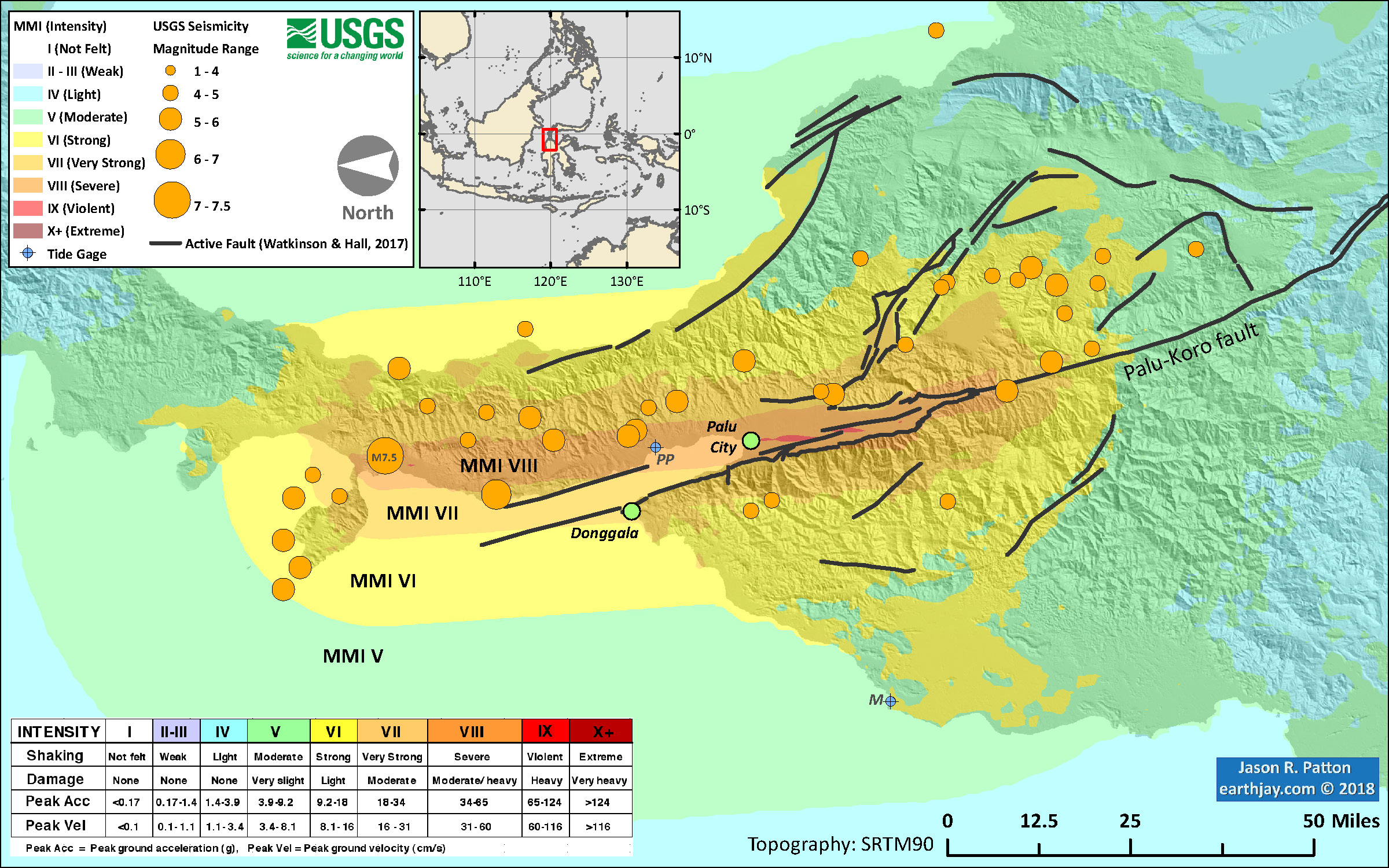
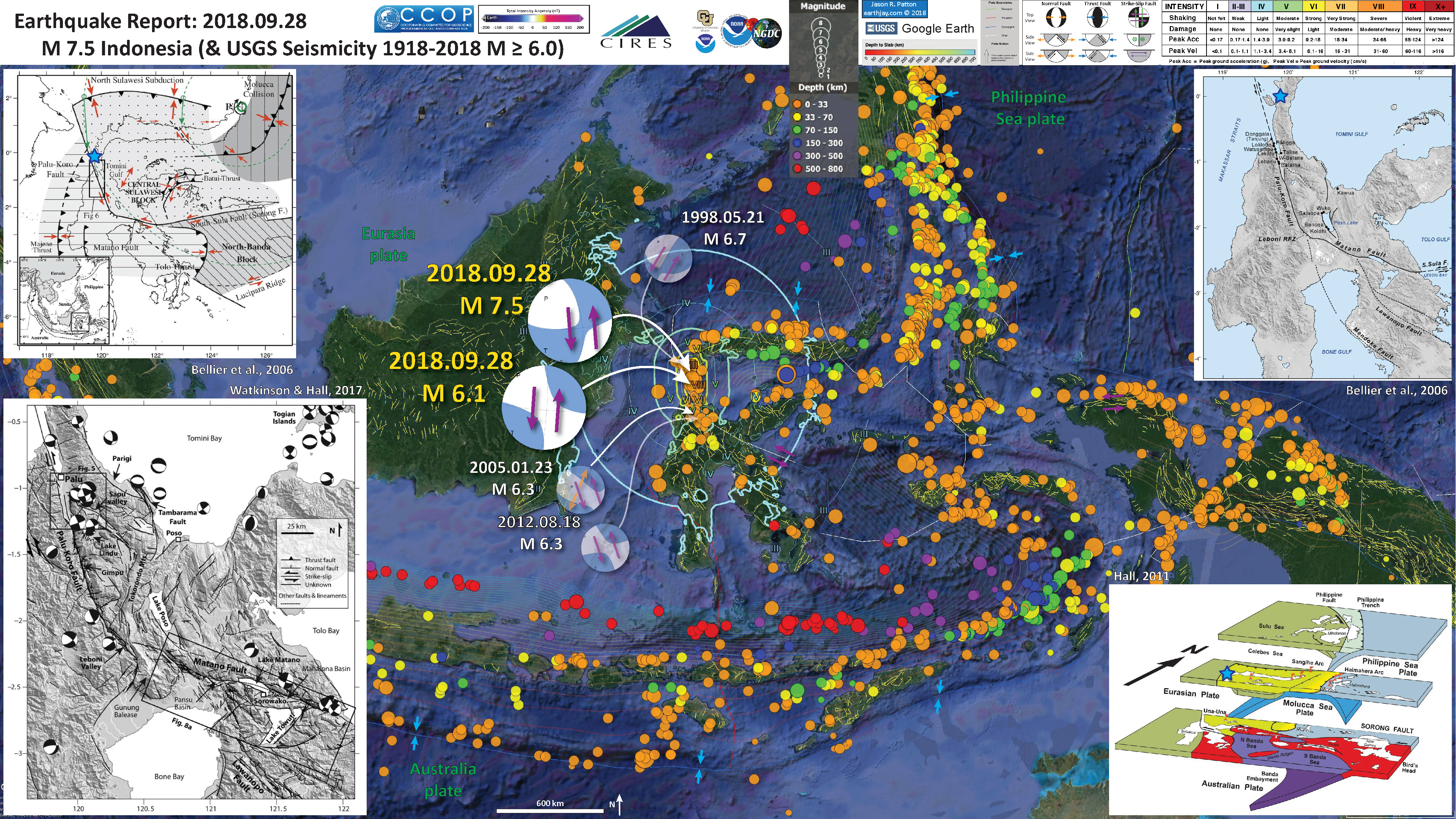
Here is the interpretive poster from my initial earthquake report. Go to the report page for more information about the seismotectonics of the region.

According to the National Disaster Management Authority (Badan Nasional Penanggulangan Bencana, BNPB), there were around 2.4 million people exposed to earthquake intensity MMI V or greater. The Modified Mercalli Intensity (MMI) scale is a measure of how strongly the ground shaking is from an earthquake. MMI V is described as, “Felt by nearly everyone; many awakened. Some dishes, windows broken. Unstable objects overturned. Pendulum clocks may stop.” However, the closer one is to the earthquake source, the greater the MMI intensity. There have been reported observations as large as MMI VIII.

Here is a map that shows the updated USGS model of ground shaking. The USGS prepared an updated earthquake fault slip model that was additionally informed by post-earthquake analysis of ground deformation. The original fault model extended from north of the epicenter to the northernmost extent of Palu City. Soon after the earthquake, Dr. Sotiris Valkaniotis prepared a map that showed large horizontal offsets across the ruptured fault along the entire length of the western margin on Palu Valley. This horizontal offset had an estimated ~8 meters of relative displacement. InSAR analyses confirmed that the coseismic ground deformation extended through Palu Valley and into the mountains to the south of the valley.

My 2018.10.01 BC Newshour Interview

Optical Analysis

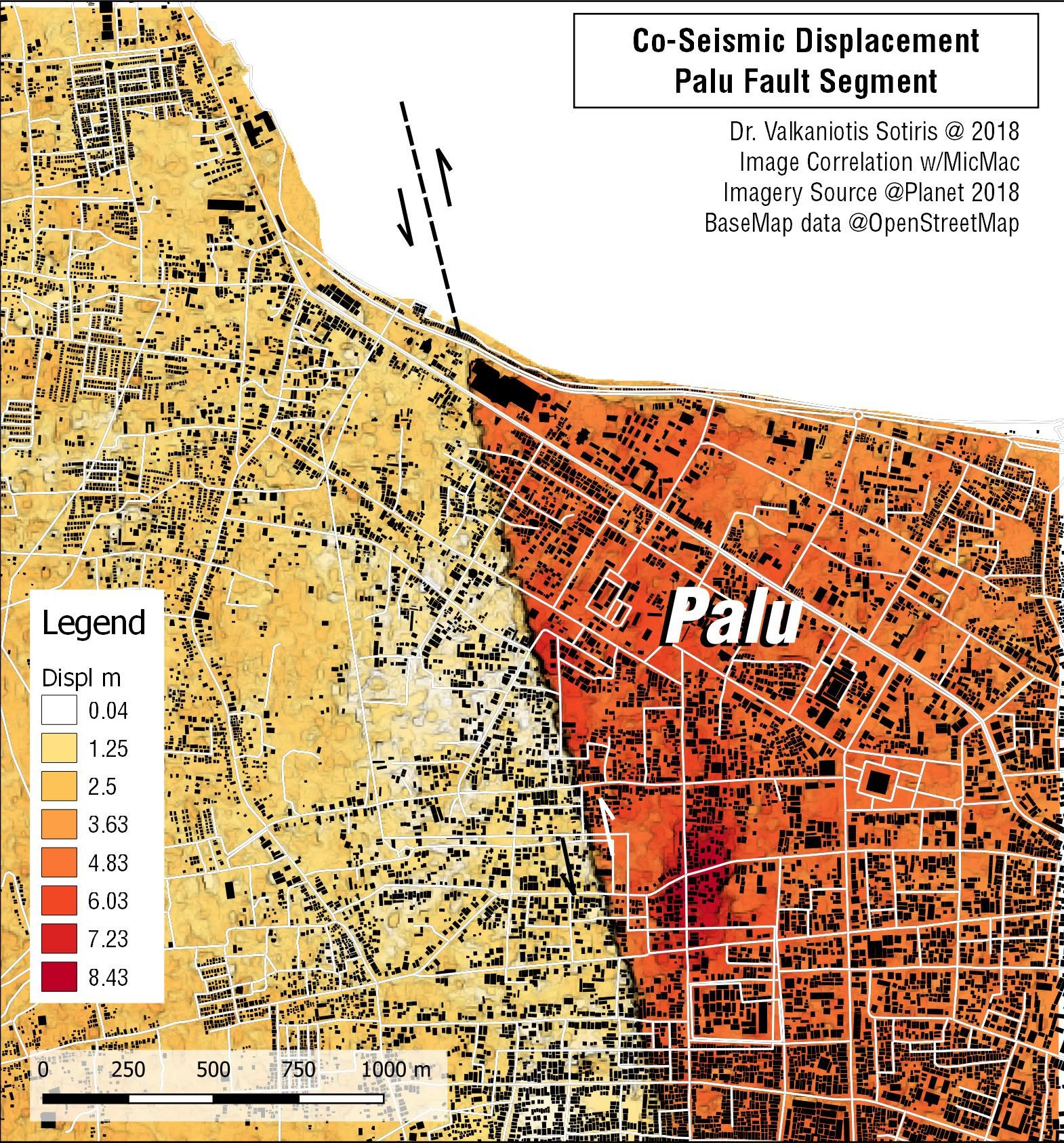
Perhaps some of the most phenomenal results from remote sensing analyses are coming from the work of Dr. Sotiris Valkaniotis. Dr. Valkaniotis has been using the open source softare mic-mac to compare pre- and post-earthquake satellite imagery. I will call this “pixel matching” analysis, or optical analysis.

Pixels are “picture elements” that comprise what a raster is created out of. Consider a television or computer monitor. The screen is displaying rows and columns of colored light. Each cell of this “raster” display is called a pixel.

Basically, the software compares the patterns in the compared imagery to detect changes. If a group of pixels in the image move relative to other pixels, then this motion is quantified. This type of analysis is particularly useful for strike-slip earthquakes as the ground moves side by side.

Dr. Valkniotis has used a variety of imagery types. Below are a couple products that they have shared on social media. Please contact Dr. Valkaniotis for more information!

This was one of the first images, showing a large displacement near the coastline in western Palu.

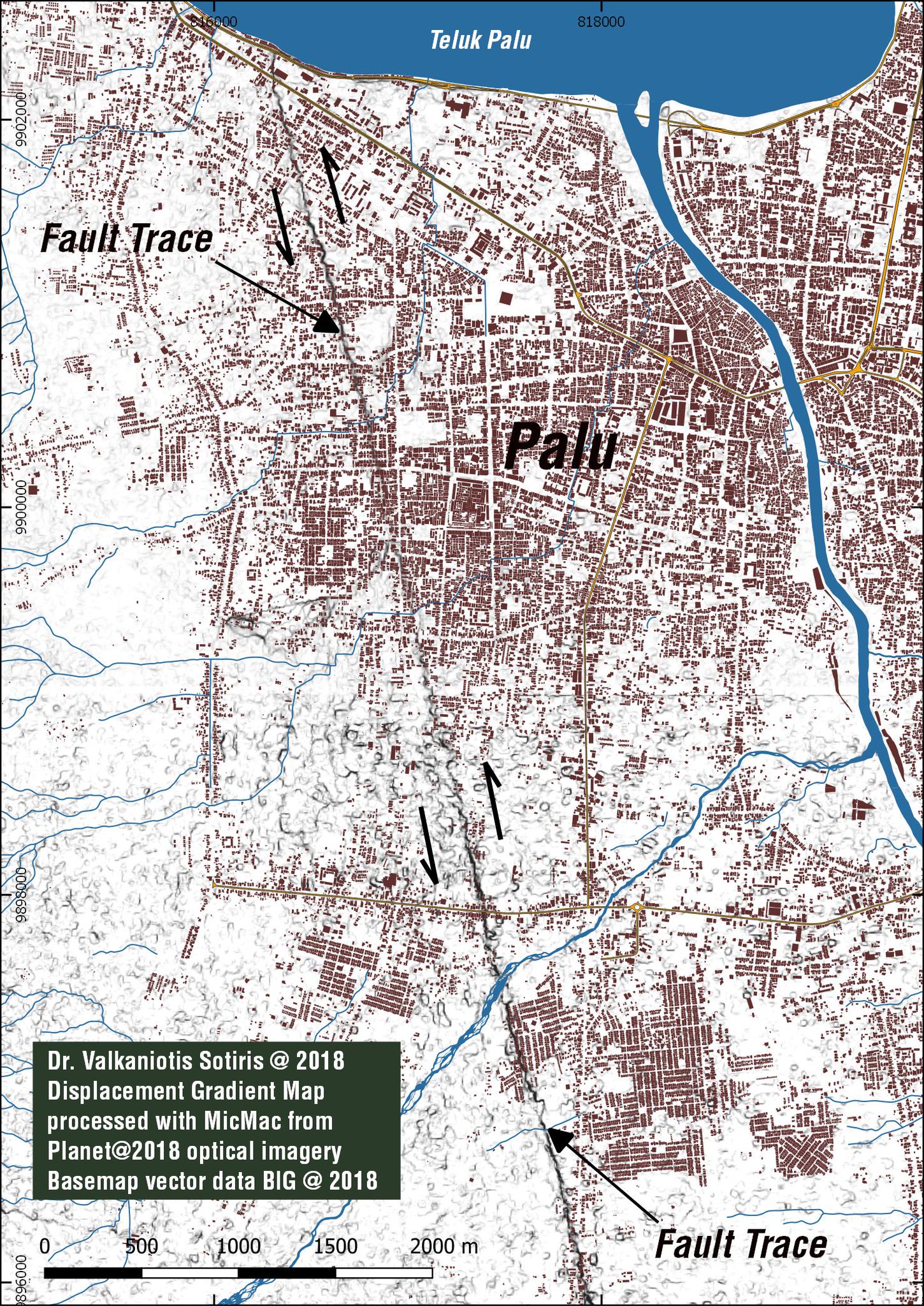
Here is another way of looking at this displacement. Valkaniotis plotted the gradient (the slope of the mic-mac displacement) to show the localized deformation from the earthquake.

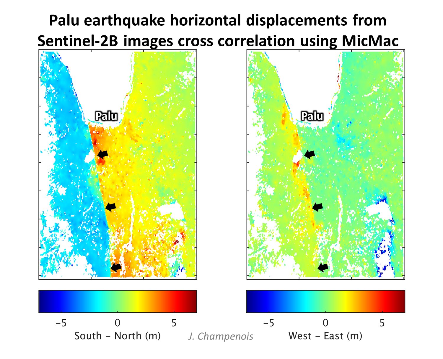
Others have used this analysis too. Here is an example from Johann Champenois who used Sentinel 2-B satellite imagery.

Here is an example that was prepared using Landsat satellite imagery conducted by Hawkeye Seismo. Here is their tweet. The left step in the Palu-Koro fault at the southern part of Palu Valley is clearly evident in this map.

Landsat-8 pixel tracking results (old school with Ampcor!) show a nice stepover in the Indonesia earthquake. This event gives a good perspective on why the valley in which Palu rests even exists in the first place

Here is a compilation from Valkaniotis, based upon Sentinel 2 imagery.

InSAR Analysis

Synthetic Aperture Radar (SAR) is a remote sensing method that uses Radar to make observations of Earth. These observations include the position of the ground surface, along with other information about the material properties of the Earth’s surface.
Interferometric SAR (InSAR) utilizes two separate SAR data sets to determine if the ground surface has changed over time, the time between when these 2 data sets were collected. More about InSAR can be found here and here. Explaining the details about how these data are analyzed is beyond the scope of this report. I rely heavily on the expertise of those who do this type of analysis, for example Dr. Eric Fielding.
Below are a series of different InSAR analytical results.

This is the result from Dr. Xiaohua Xu, prepared on 2018.10.15

Line-of-sight deformation from ALOS-2 for the Palu earthquake (data provided by JAXA, processed using GMTSAR). Unwrapping is challenging for this earthquake! Some near-fault region is too decorrelated to be trustworthy.

Below are 2 results from Dr. Fielding.

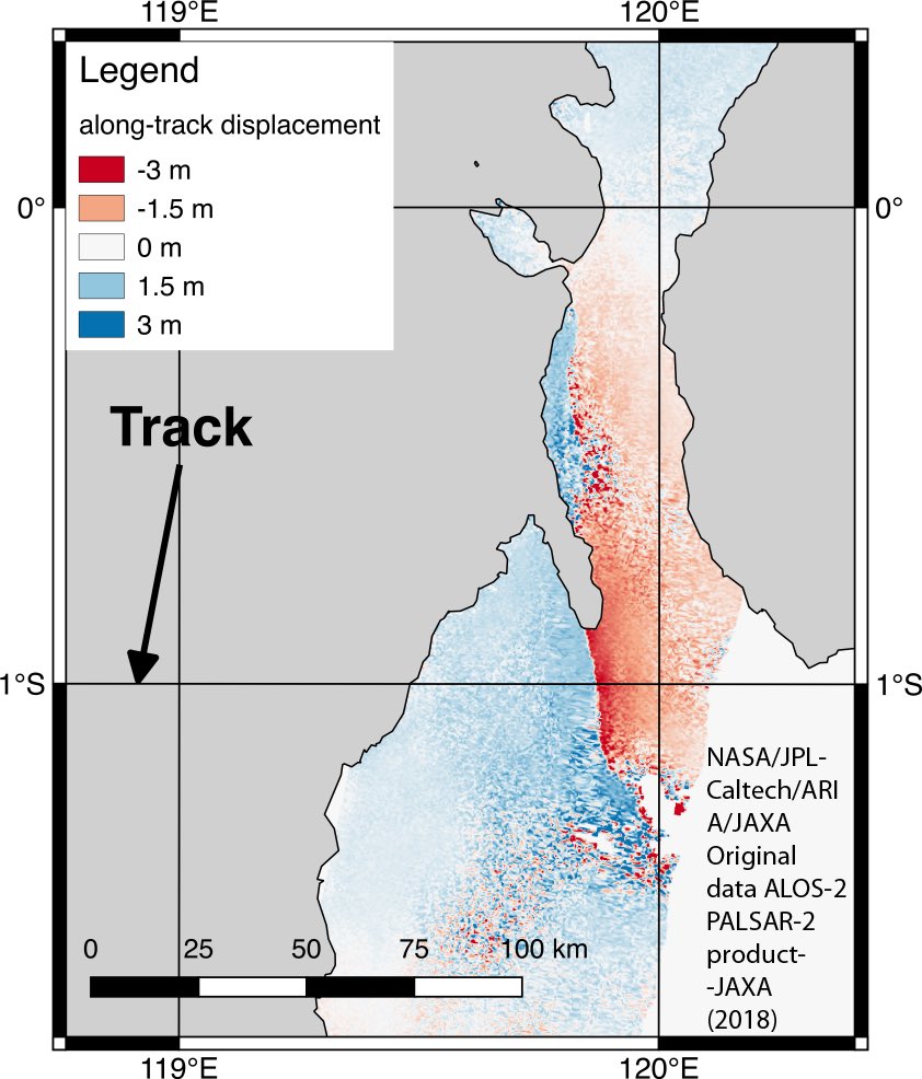
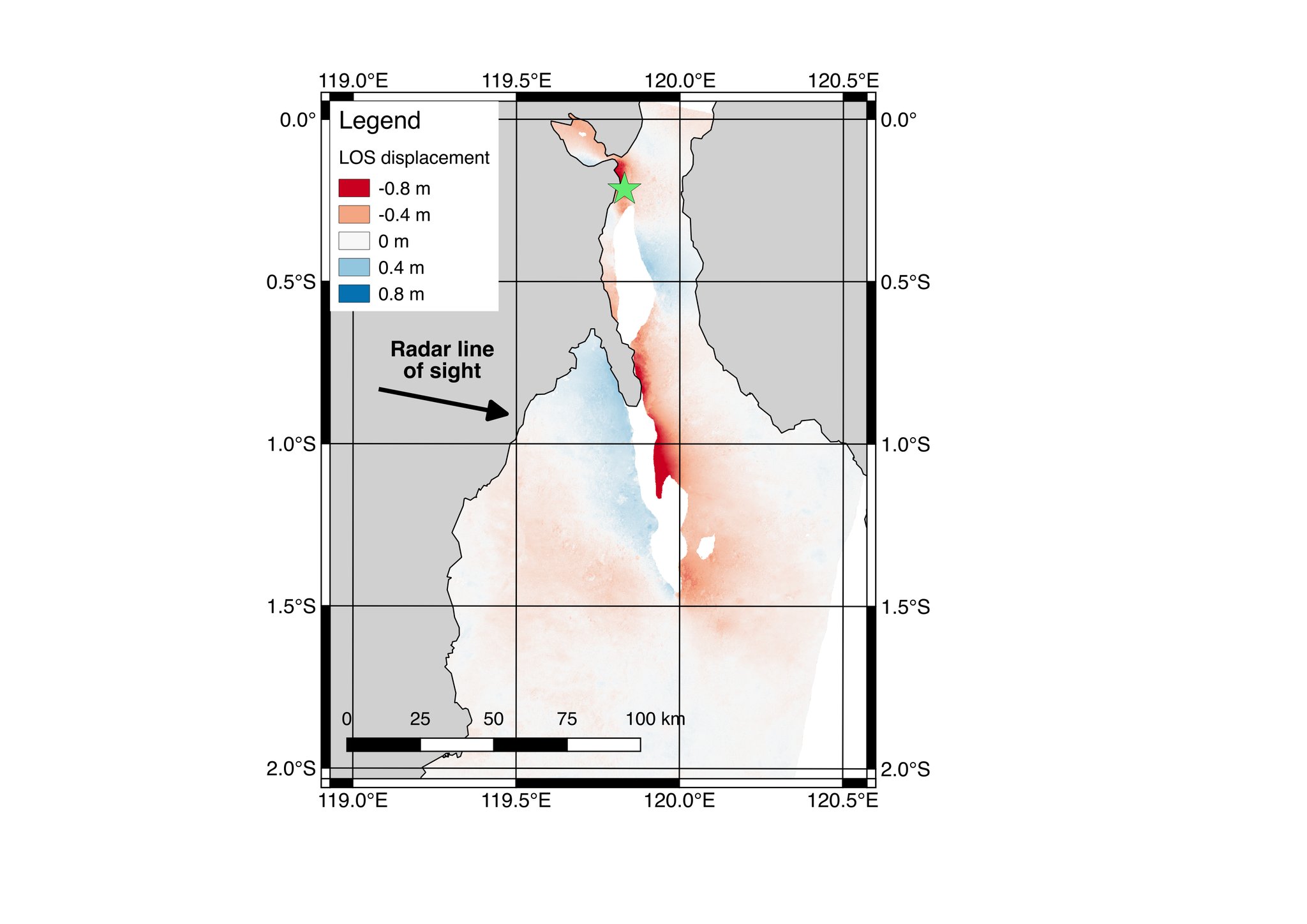
#InSAR map of range or line-of-sight deformation of #PaluEarthquake from NASA Caltech-JPL analysis of JAXA ALOS-2 PALSAR-2 data acquired last week. Red areas moved west or down in this unwrapped interferogram, unreliable phase masked out. Star USGS epicenter.

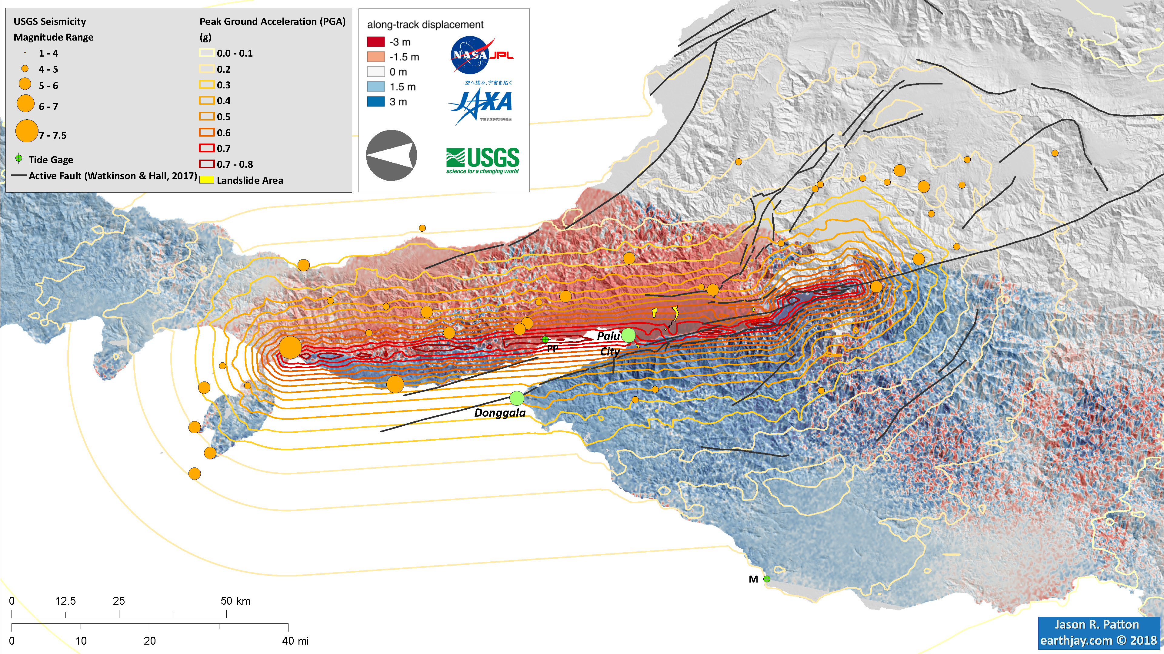
I prepared a map using the NASA-JPL InSAR data. They post all their data online here. I used the tiff image as it is georeferenced. However, some may prefer to use the kmz file in Google Earth.
I include the faults mapped by Wilkinson and Hall (2017), the PGA contours from the USGS model results. More on Peak Ground Acceleration (PGA) can be found here. I also include the spatial extent of the largest landslides that I mapped using post-earthquake satellite imagery provided by Digital Globe using their open source imagery program.

Tsunami

There have been observations of tsunami waves recorded by tide gages installed at Pantoloan Port and Mumuju, Sulawesi. Locations are shown on the map above. A tsunami with a 10 cm wave height was recorded at Mumuju tide gage and a wave with a height of about 1.7 meters was recorded at Pantoloan tide gage. Learn more about the tsunami here.
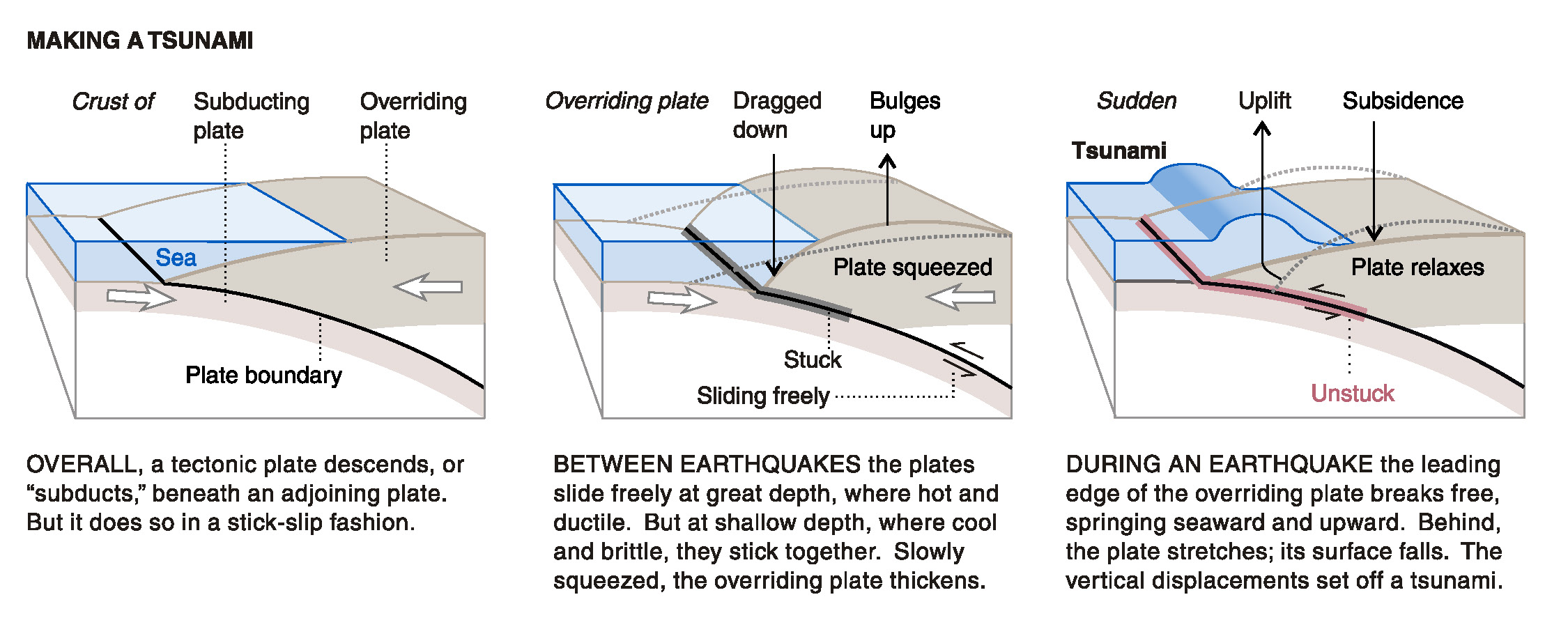
Tsunami can be caused by a variety of processes, including earthquakes, volcanic eruptions, landslides, and meteorological phenomena. Earthquakes, eruptions, and landslides cause tsunami when these processes displace water in some way. We may typically associate tsunami with subduction zone earthquakes because these earthquakes are the type that generate vertical land motion along the sea floor. However, we know that strike-slip earthquakes can also generate tsunami (e.g. the 1999 Izmit, Turkey earthquake). But strike-slip earthquakes typically generate tsunami that are smaller in size.

Here is a great illustration of how a subduction zone earthquake can generate a tsunami (Atwater et al., 2005).

When landslides generate tsunami, they are often localized relative to the location of the landslide. The tsunami size can be rather large near the landslide and the size diminishes rapidly with distance from the landslide. An example of a landslide generated tsunami is the 1998 Papua New Guinea tsunami (an earthquake triggered a landslide, causing a “larger than expected” tsunami to inundate the land there. The size of the tsunami was very large near the landslide.
Based on post-earthquake satellite imagery from Digital Globe, the overwhelming majority of tsunami damage is localized within Palu Bay. The severity of damage is worse in southern Palu Bay where tsunami inundation is on the order of 300 feet. While at the northern part of the bay, inundation is on the order of 50 feet. In the north, most of the buildings that were destroyed by the tsunami were built over the water, though not entirely. While in the south, building damage extends further inland where buildings have been destroyed that were not built over the water. North of the mouth of the bay, there is less evidence for tsunami inundation, but there is localized damage in places.
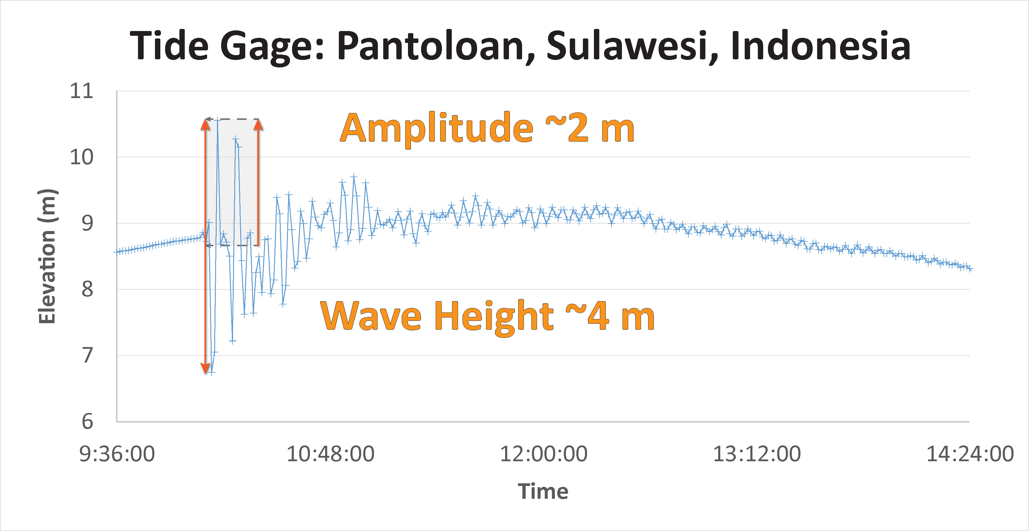
There was a tsunami recorded at the Pantoloan Port tide gage with an amplitude of about 1 meter. At this location is also a 50 long ship that was lifted up onto a dock at the port. More details about the observations made by the joint Indonesia/Japan post-tsunami survey team cab be found at Temblor here.

Here is my plot of the Pantoloan Port tide gage.

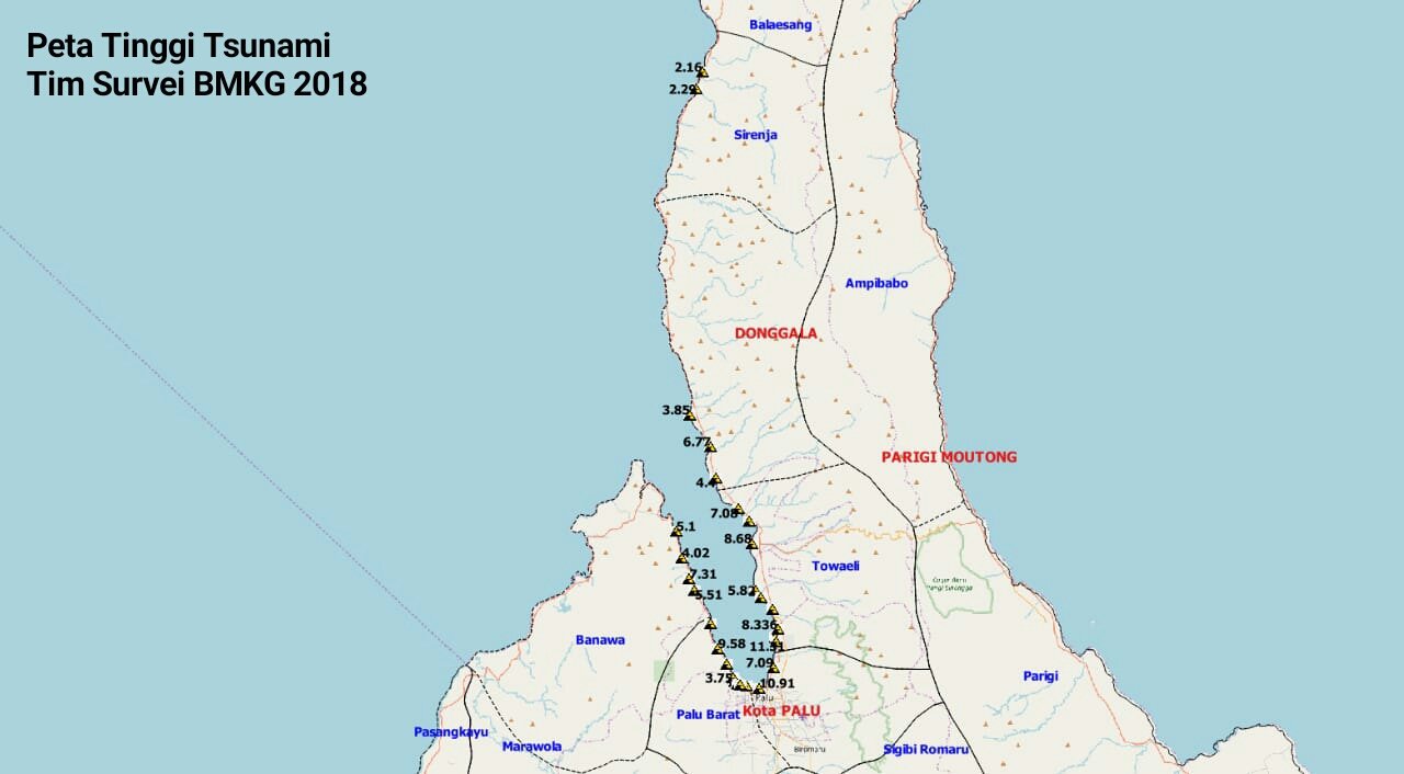
Here is a map that shows the preliminary results from the field survey. These elevation data are better explained in their report.

M 7.5 Landslide Model vs. Observation Comparison

Landslides during and following the M=7.5 earthquake in central Sulawesi, Indonesia possibly caused the majority of casualties from this catastrophic natural disaster. Volunteers (citizen scientists) have used satellite aerial imagery collected after the earthquake to document the spatial extent and magnitude of damage caused by the earthquake, landslides, and tsunami.

While remote sensing methods are useful to locate damage in the region, field observations will be key in the effort to analyze the landscape response to these natural disasters. The Indonesian government and international researchers are already surveying the region and collecting these important observational details.

There are many different ways in which a landslide can be triggered. The first order relations behind slope failure (landslides) is that the “resisting” forces that are preventing slope failure (e.g. the strength of the bedrock or soil) are overcome by the “driving” forces that are pushing this land downwards (e.g. gravity). The ratio of resisting forces to driving forces is called the Factor of Safety (FOS). We can write this ratio like this:

FOS = Resisting Force / Driving Force

When FOS > 1, the slope is stable and when FOS < 1, the slope fails and we get a landslide. The illustration below shows these relations. Note how the slope angle α can take part in this ratio (the steeper the slope, the greater impact of the mass of the slope can contribute to driving forces). The real world is more complicated than the simplified illustration below.

Landslide ground shaking can change the Factor of Safety in several ways that might increase the driving force or decrease the resisting force. Keefer (1984) studied a global data set of earthquake triggered landslides and found that larger earthquakes trigger larger and more numerous landslides across a larger area than do smaller earthquakes.

Earthquakes can cause landslides because the seismic waves can cause the driving force to increase (the earthquake motions can “push” the land downwards), leading to a landslide. In addition, ground shaking can change the strength of these earth materials (a form of resisting force) with a process called liquefaction.

Sediment or soil strength is based upon the ability for sediment particles to push against each other without moving. This is a combination of friction and the forces exerted between these particles. This is loosely what we call the “angle of internal friction.” Liquefaction is a process by which pore pressure increases cause water to push out against the sediment particles so that they are no longer touching.

An analogy that some may be familiar with relates to a visit to the beach. When one is walking on the wet sand near the shoreline, the sand may hold the weight of our body generally pretty well. However, if we stop and vibrate our feet back and forth, this causes pore pressure to increase and we sink into the sand as the sand liquefies. Or, at least our feet sink into the sand.

Below is a diagram showing how an increase in pore pressure can push against the sediment particles so that they are not touching any more. This allows the particles to move around and this is why our feet sink in the sand in the analogy above. This is also what changes the strength of earth materials such that a landslide can be triggered.

Below is a diagram based upon a publication designed to educate the public about landslides and the processes that trigger them (USGS, 2004). Additional background information about landslide types can be found in Highland et al. (2008). There was a variety of landslide types that can be observed surrounding the earthquake region. So, this illustration can help people when they observing the landscape response to the earthquake whether they are using aerial imagery, photos in newspaper or website articles, or videos on social media. Will you be able to locate a landslide scarp or the toe of a landslide? This figure shows a rotational landslide, one where the land rotates along a curvilinear failure surface.

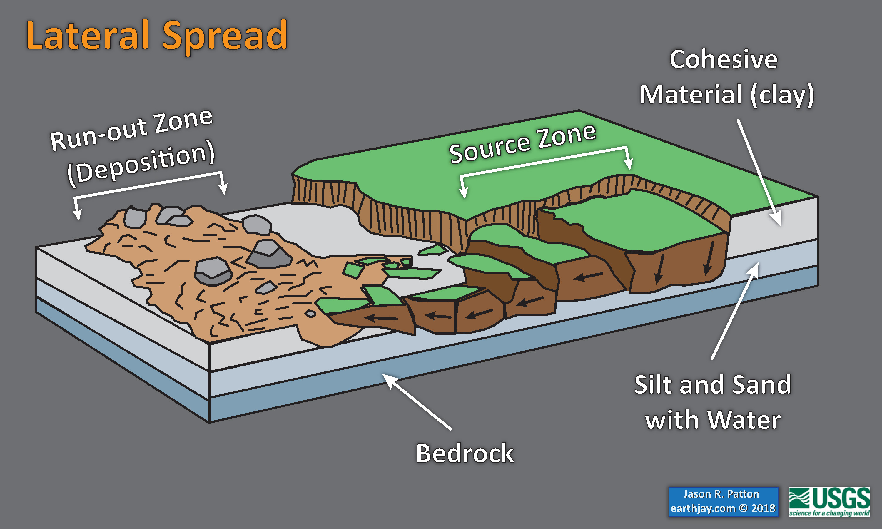
A lateral spread is a translational landslide that occurs over gentle slopes or flat terrain. The failure surface is more planar and less curvy than for rotational slides. The spread is usually caused when a confined layer of sediment is transformed from a solid into a liquid state. In the lateral spread figure below, it is the water that exists in the “silt and sand” deposits that has an increase in pore pressure to generate liquefaction, causing the failure. The overlying sediment is more cohesive, which is why we may have seen landslides move as coherent blocks across the landscape. However, these landslide blocks may disaggregate as they move, sometimes turning into a flow. This entire range of behavior can be seen in the post-earthquake aerial imagery of Palu Valley.

Here is an excellent educational video from IRIS and a variety of organizations. The video helps us learn about how earthquake intensity gets smaller with distance from an earthquake. The concept of liquefaction is reviewed and we learn how different types of bedrock and underlying earth materials can affect the severity of ground shaking in a given location. The intensity map above is based on a model that relates intensity with distance to the earthquake, but does not incorporate changes in material properties as the video below mentions is an important factor that can increase intensity in places.

If we look at the map at the top of this report, we might imagine that because the areas close to the fault shake more strongly, there may be more landslides in those areas. This is probably true at first order, but the variation in material properties and water content also control where landslides might occur.

There has been a large amount of videos posted online via social media and professional news organizations showing the impact of these landslides. Perhaps one of the best places to seek an expert informed view of landslide processes, of all types, is from Dr. David Petley and his blog, The Landslide Blog. Petley has presented a couple summaries of these observations of coseismic (during the earthquake) landslides as triggered by ground shaking from the M=7.5 Donggala earthquake.

The company Digital Globe provides high resolution satellite imagery for a fee, but they distribute imagery for free via their open data program following natural disasters. This imagery is available for noncommercial use including disaster impact analysis. Many of the preliminary analyses of impact presented on social media by subject matter experts has been based upon this imagery. Another source of fee based imagery is from Planet Lab that also provides imagery in support of peoples’ response to natural disasters via their disaster data program.

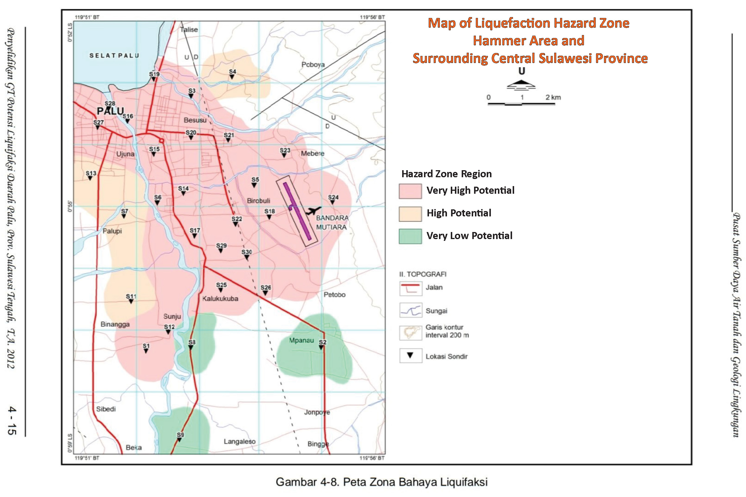
Most of the entire Palu Valley has previously been mapped as susceptible to liquefaction due to (1) the underlying materials are sediments and (2) a shallow ground water table (lots of water in the sediment, reaching close to the ground surface). The northern part of the valley is a river delta full of loose and water saturated sediments. Yet, only a small portion of the entire valley failed as these km scale lateral spreads.

Why is this? This is probably due to a combination of factors, but the biggest factor may be the heterogeneity of the underlying earth materials. These sediments probably have variation in material properties: strength (“angle of internal friction“), stickiness (“cohesion“), and porosity (spaces between sediment particles that can be filled with water).

Below is the liquefaction susceptibility map prepared in 2012. I just noticed that one of the 2 largest landslides actually happened outside of these liquefaction zones.

It is also possible that the earthquake intensity (ground shaking and seismic wave energy), that was directed in different directions, may have caused different amounts of “seismic loading” of these slopes.

Knowing how these material properties vary spatially is difficult to know as the materials in the subsurface are generally not in plain view (buried under ground). People can drill and sample the material properties (an engineering geologist) and then calculate the strength of these materials (engineer) on a site by site basis.

Until these landslides are analyzed and compared with regions that did not fail in slope failure, we will not be able to reconstruct what happened… why some areas failed and some did not.

There are landslide slope stability and liquefaction susceptibility models based on empirical data from past earthquakes. The USGS has recently incorporated these types of analyses into their earthquake event pages. More about these USGS models can be found on this page.

I prepared some maps that compare the USGS landslide and liquefaction probability maps. Below I present these results along with the MMI contours. I also include the faults mapped by Wilkinson and Hall (2017). Shown are the cities of Donggala and Palu. Also shown are the 2 tide gage locations (Pantoloan Port – PP and Mumuju – M). I also used post-earthquake satellite imagery to outline the largest landslides in Palu Valley, ones that appear to be lateral spreads.

Here is the landslide probability map (Jessee et al., 2018). Below the poster I include the text from the USGS website that describes how this model is prepared.

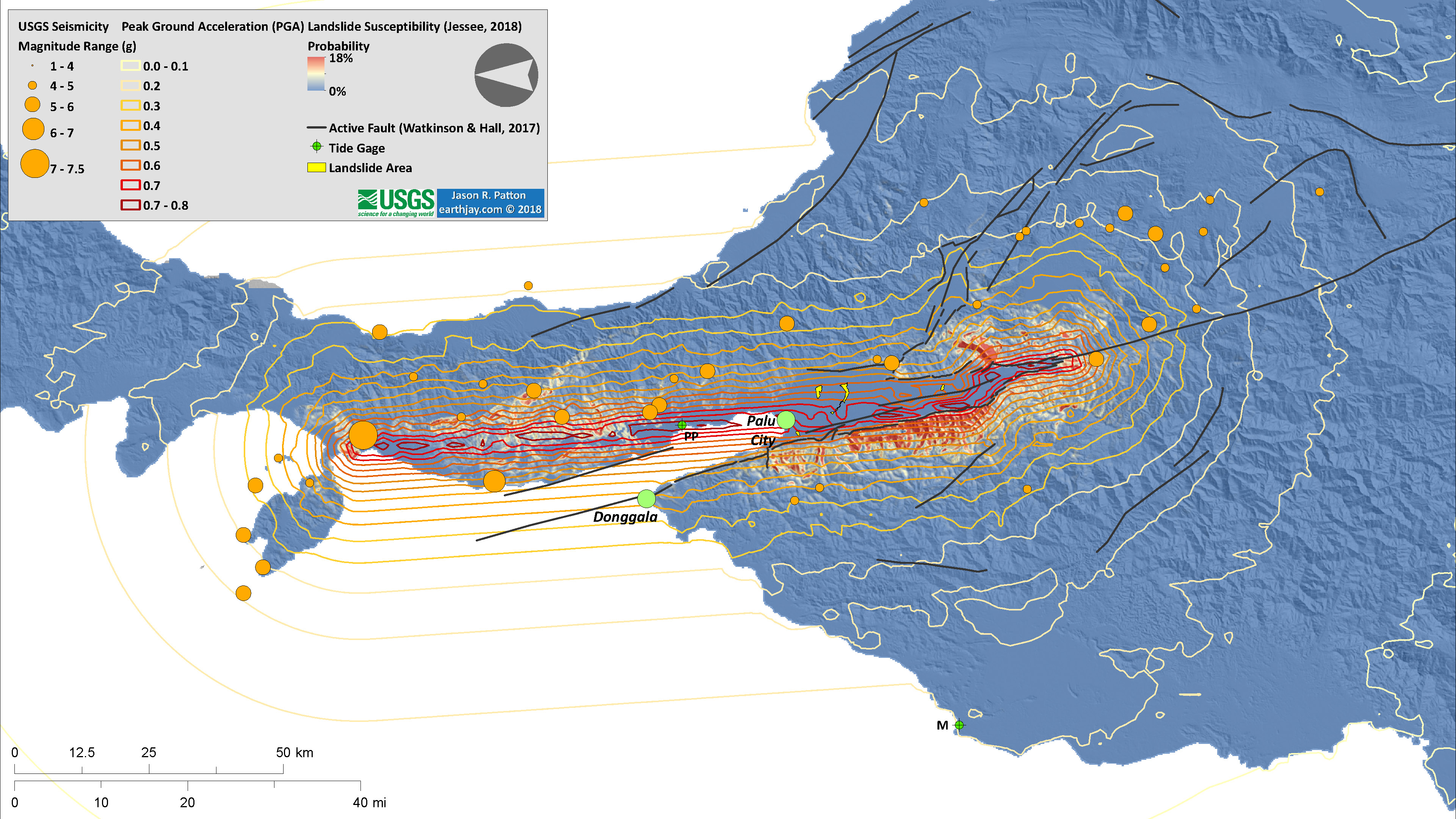
Nowicki Jessee and others (2018) is the preferred model for earthquake-triggered landslide hazard. Our primary landslide model is the empirical model of Nowicki Jessee and others (2018). The model was developed by relating 23 inventories of landslides triggered by past earthquakes with different combinations of predictor variables using logistic regression. The output resolution is ~250 m. The model inputs are described below. More details about the model can be found in the original publication. We modify the published model by excluding areas with slopes <5° and changing the coefficient for the lithology layer "unconsolidated sediments" from -3.22 to -1.36, the coefficient for "mixed sedimentary rocks" to better reflect that this unit is expected to be weak (more negative coefficient indicates stronger rock).To exclude areas of insignificantly small probabilities in the computation of aggregate statistics for this model, we use a probability threshold of 0.002.

Here is the liquefaction probability (susceptibility) map (Zhu et al., 2017). Note that the regions of low slopes in the valleys and coastal plains are the areas with a high chance of experiencing liquefaction. Areas of slopes >5° are excluded from this analysis.
Note that the large landslides (yellow polygons) are not in regions of high probability for liquefaction.

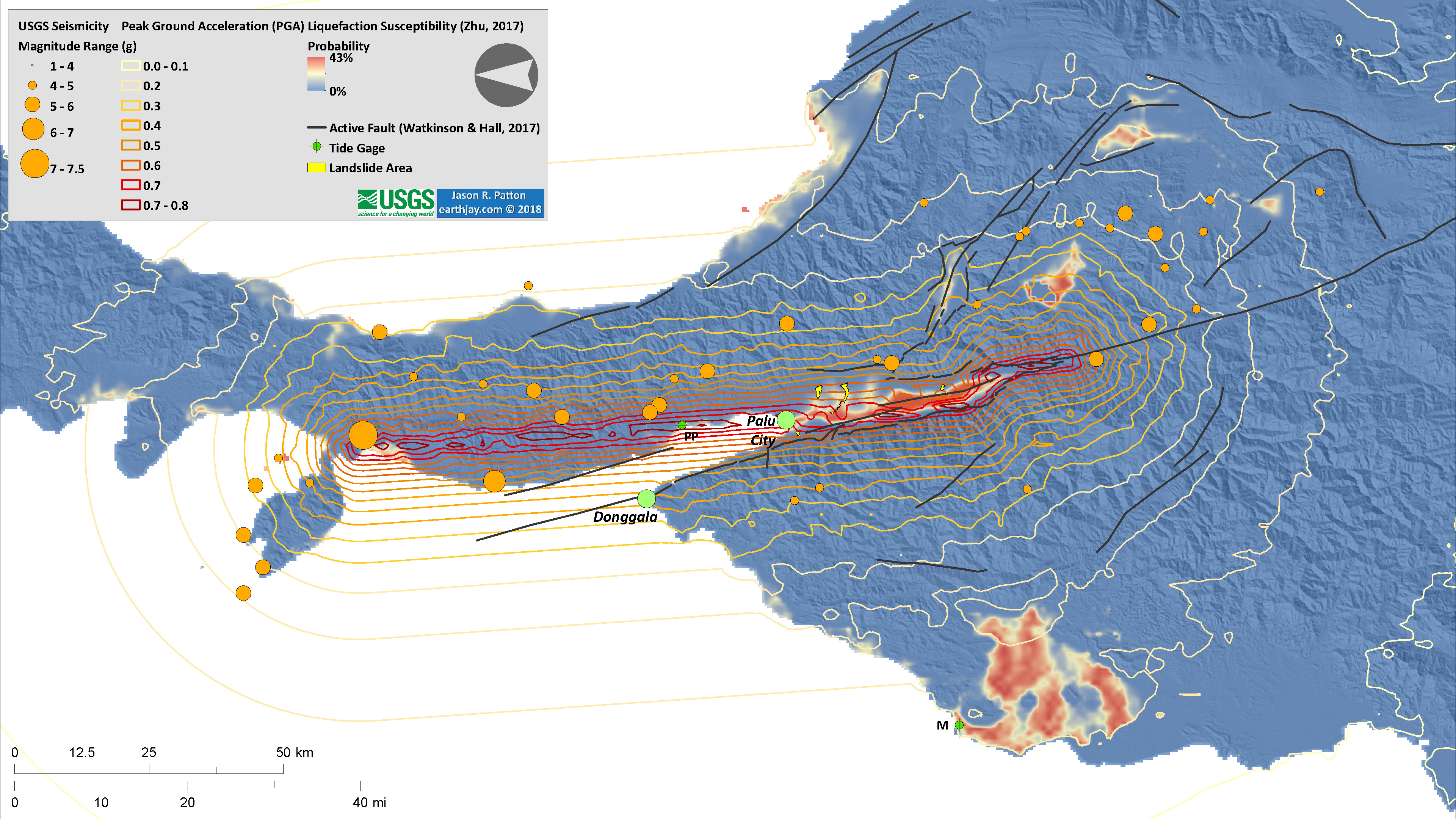
Zhu and others (2017) is the preferred model for liquefaction hazard. The model was developed by relating 27 inventories of liquefaction triggered by past earthquakes to globally-available geospatial proxies (summarized below) using logistic regression. We have implemented the global version of the model and have added additional modifications proposed by Baise and Rashidian (2017), including a peak ground acceleration (PGA) threshold of 0.1 g and linear interpolation of the input layers. We also exclude areas with slopes >5°. We linearly interpolate the original input layers of ~1 km resolution to 500 m resolution. The model inputs are described below. More details about the model can be found in the original publication.

References:

Atwater, B.F., Musumi-Rokkaku, S., Satake, K., Tsuju, Y., Eueda, K., and Yamaguchi, D.K., 2005. The Orphan Tsunami of 1700—Japanese Clues to a Parent Earthquake in North America, USGS Professional Paper 1707, USGS, Reston, VA, 144 pp.
Cipta, A., Robiana, R., Griffin, J.D., Horspool, N., Hidayati, S., and Cummins, P., 2016. A probabilistic seismic hazard assessment for Sulawesi, Indonesia in Cummins, P. R. &Meilano, I. (eds) Geohazards in Indonesia: Earth Science for Disaster Risk Reduction, Geological Society, London, Special Publications, v. 441, http://doi.org/10.1144/SP441.6
Gómez, J.M., Madariaga, R., Walpersdorf, A., and Chalard, E., 2000. The 1996 Earthquakes in Sulawesi, Indonesia in BSSA, v. 90, no. 3, p. 739-751
Highland, L.M., and Bobrowsky, P., 2008. The landslide handbook—A guide to understanding landslides, Reston, Virginia, U.S. Geological Survey Circular 1325, 129 p.
Jessee, M.A.N., Hamburger, M. W., Allstadt, K., Wald, D. J., Robeson, S. M., Tanyas, H., et al. (2018). A global empirical model for near-real-time assessment of seismically induced landslides. Journal of Geophysical Research: Earth Surface, 123, 1835–1859. https://doi.org/10.1029/2017JF004494
Keefer, D.K., 1984. Landslides Caused by Earthquakes in GSA Bulletin, v. 95, p. 406-421
Socquet, A., Simons, W., Vigny, C., McCaffrey, R., Subarya, C., Sarsito, D., Ambrosius, B., and Spakman, W., 2006. Microblock rotations and fault coupling in SE Asia triple junction (Sulawesi, Indonesia) from GPS and earthquake slip vector data, J. Geophys. Res., 111, B08409, doi:10.1029/2005JB003963.
USGS, 2004. Landslide Types and Processes, U.S. Geological Survey Fact Sheet 2004-3072
Watkinson, I.M. and Hall, R., 2017. Fault systems of the eastern Indonesian triple junction: evaluation of Quaternary activity and implications for seismic hazards in Cummins, P. R. & Meilano, I. (eds) Geohazards in Indonesia: Earth Science for Disaster Risk Reduction, Geological Society, London, Special Publications, v. 441, https://doi.org/10.1144/SP441.8
Zhu, J., Baise, L. G., Thompson, E. M., 2017, An Updated Geospatial Liquefaction Model for Global Application, Bulletin of the Seismological Society of America, 107, p 1365-1385, doi: 0.1785/0120160198