This region of Earth is one of the most seismically active in the past decade plus. This morning, as I was preparing for work, I got an email notifying me of an earthquake with a magnitude M = 7.5 located near New Ireland, Papua New Guinea.
https://earthquake.usgs.gov/earthquakes/eventpage/us70003kyy/executive
There are every type of plate boundary fault in this region. There are subduction zones, such as that forms the New Britain and San Cristobal trenches. There are transform faults, such as that responsible for the M 7.5 temblor. There are also spreading ridges, such as the one that forms the Manus Basin to the northwest of today’s quake.
I interpret this M 7.5 earthquake to be a left-lateral strike slip earthquake based on (1) the USGS mechanism (moment tensor), (2) our knowledge of the faulting in the region, and (3) historic analogue earthquake examples. There was an earthquake on a subparallel strike-slip fault on 8 March 2018 (here is the earthquake report for that event). Also in that report, I discuss an earthquake from November 2000 that had a magnitude M = 8.0.
After my work on the 28 September 2018 Donggala-Palu earthquake, landslides, and tsunami, I am open minded about the possibility of strike-slip earthquakes as having tsunamigenic potential. There are actually many examples of strike-slip earthquakes causing tsunami, including the 1999 Izmit, 2012 Wharton Basin, and the 2000 New Ireland earthquake too! (see Geist and Parsons, 2005 for more about the small 2000 tsunami.) There was initially a tsunami notification from tsunami.gov about the possibility of a tsunami. Here is a great website where I usually visit when I am looking for tsunami records on tide gage data. This is the closest gage to the quake, but it is not located optimally to record a small tsunami as might have been generated today (I checked).
The Weitin fault is a very active fault, with a slip rate of about 130 mm/yr (Tregoning et al, 1999, 2005). For a comparison, the San Andreas fault has a slip rate of about 25-35 mm/year. Here is a great treatise on the SAF.
There are also examples of earthquake triggering in this region. For example, the 2000.11.16 M 8.0 strike-slip earthquake triggered the 2000.11.16 M 7.8 thrust fault earthquake. It is not unreasonable to consider it possible that there may be triggered earthquakes from this M 7.5 earthquake. Of course, we won’t know until it happens because nobody has the capability to predict earthquakes (regardless of what the charlatans may claim).
The USGS has a variety of products associated with their earthquake pages. I use many of these products in these earthquake reports, so I especially appreciate them. One of the recently added products is a landslide and a liquefaction probability model output. Based on our knowledge of how earthquake release energy, and our knowledge of how earth materials respond to this energy release, people have developed models that allow us to estimate the possibility any given region may experience landslides or liquefaction. I spent some time discussing this in the 28 Sept. 2018 Donggala-Palu earthquake report here.
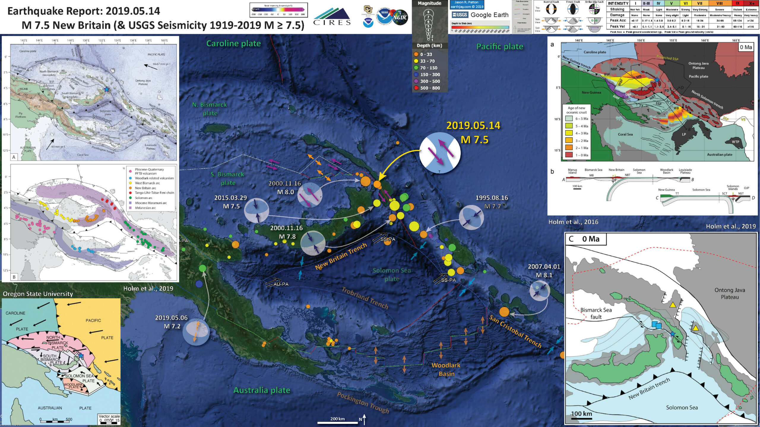
Below is my interpretive poster for this earthquake
I plot the seismicity from the past month, with color representing depth and diameter representing magnitude (see legend). I include earthquake epicenters from 1918-2018 with magnitudes M ≥ 3.0 in one version.
I plot the USGS fault plane solutions (moment tensors in blue and focal mechanisms in orange), possibly in addition to some relevant historic earthquakes.
- I placed a moment tensor / focal mechanism legend on the poster. There is more material from the USGS web sites about moment tensors and focal mechanisms (the beach ball symbols). Both moment tensors and focal mechanisms are solutions to seismologic data that reveal two possible interpretations for fault orientation and sense of motion. One must use other information, like the regional tectonics, to interpret which of the two possibilities is more likely.
- I also include the shaking intensity contours on the map. These use the Modified Mercalli Intensity Scale (MMI; see the legend on the map). This is based upon a computer model estimate of ground motions, different from the “Did You Feel It?” estimate of ground motions that is actually based on real observations. The MMI is a qualitative measure of shaking intensity. More on the MMI scale can be found here and here. This is based upon a computer model estimate of ground motions, different from the “Did You Feel It?” estimate of ground motions that is actually based on real observations.
- I include the slab 2.0 contours plotted (Hayes, 2018), which are contours that represent the depth to the subduction zone fault. These are mostly based upon seismicity. The depths of the earthquakes have considerable error and do not all occur along the subduction zone faults, so these slab contours are simply the best estimate for the location of the fault.
- In the map below, I include a transparent overlay of the magnetic anomaly data from EMAG2 (Meyer et al., 2017). As oceanic crust is formed, it inherits the magnetic field at the time. At different points through time, the magnetic polarity (north vs. south) flips, the North Pole becomes the South Pole. These changes in polarity can be seen when measuring the magnetic field above oceanic plates. This is one of the fundamental evidences for plate spreading at oceanic spreading ridges (like the Gorda rise).
- Regions with magnetic fields aligned like today’s magnetic polarity are colored red in the EMAG2 data, while reversed polarity regions are colored blue. Regions of intermediate magnetic field are colored light purple.
- We can see the roughly east-west trends of these red and blue stripes in the Woodlark Basin. These lines are parallel to the ocean spreading ridges from where they were formed. The stripes disappear at the subduction zone because the oceanic crust with these anomalies is diving deep beneath the upper plate, so the magnetic anomalies from the overlying plate mask the evidence for the lower plate.
Magnetic Anomalies
- In the lower left corner is a figure from Oregon State University (Geology). This shows a cartoon view of the tectonic plates in the region. Note the subduction zone where the Solomon Sea late dives beneath the South Bismarck and Pacific plates. Of particular interest today is the transform (strike-slip) plate boundary between the North and South Bismarck plates.
- In the upper left corner are two more detailed tectonic maps from Holm et al. (2019). The upper panel shows the plate boundary faults (active subduction zones are symbolized with dark triangles, fossil subd. zones are shown as open triangles). I plate a blue star int eh location of today’s earthquake (as for all inset figures). The lower panel shows the source of volcanic rocks as they have been derived from different subducted oceanic crust and overlying mantle. The geochemistry of these volcanic rocks helps us learn about the tectonic history of this complicated region.
- The figure in the lower right corner (Holm et al., 2019) shows the current configuration of the different plate boundary faults. Note the left lateral strike-slip relative motion on the (labeled here) Bismarck Sea fault. When this fault crosses New Ireland, it splays into a series of different faults. The most active fault is the Weitin fault.
- The figure in the upper right corner has lots of information, including cross sections showing the subduction zones (Holm et al., 2016). The oceanic crust created by spreading centers is highlighted for the Woodlark Basin, as well as the Manus Basin northwest of today’s M 7.5 earthquake. The cross section A-B shows these spreading centers.
I include some inset figures. Some of the same figures are located in different places on the larger scale map below.
- Here is the map with a month’s seismicity plotted. This map includes magnetic anomaly data.

- Here is the map with a century’s seismicity plotted for magnitudes M ≥ 7.5. Because of the complexity of this figure, the magnetic anomaly data are not included.

M 7.5 Landslide and Liquefaction Models
There are many different ways in which a landslide can be triggered. The first order relations behind slope failure (landslides) is that the “resisting” forces that are preventing slope failure (e.g. the strength of the bedrock or soil) are overcome by the “driving” forces that are pushing this land downwards (e.g. gravity). The ratio of resisting forces to driving forces is called the Factor of Safety (FOS). We can write this ratio like this:
FOS = Resisting Force / Driving Force
When FOS > 1, the slope is stable and when FOS < 1, the slope fails and we get a landslide. The illustration below shows these relations. Note how the slope angle α can take part in this ratio (the steeper the slope, the greater impact of the mass of the slope can contribute to driving forces). The real world is more complicated than the simplified illustration below.

Landslide ground shaking can change the Factor of Safety in several ways that might increase the driving force or decrease the resisting force. Keefer (1984) studied a global data set of earthquake triggered landslides and found that larger earthquakes trigger larger and more numerous landslides across a larger area than do smaller earthquakes. Earthquakes can cause landslides because the seismic waves can cause the driving force to increase (the earthquake motions can “push” the land downwards), leading to a landslide. In addition, ground shaking can change the strength of these earth materials (a form of resisting force) with a process called liquefaction.
Sediment or soil strength is based upon the ability for sediment particles to push against each other without moving. This is a combination of friction and the forces exerted between these particles. This is loosely what we call the “angle of internal friction.” Liquefaction is a process by which pore pressure increases cause water to push out against the sediment particles so that they are no longer touching.
An analogy that some may be familiar with relates to a visit to the beach. When one is walking on the wet sand near the shoreline, the sand may hold the weight of our body generally pretty well. However, if we stop and vibrate our feet back and forth, this causes pore pressure to increase and we sink into the sand as the sand liquefies. Or, at least our feet sink into the sand.
Below is a diagram showing how an increase in pore pressure can push against the sediment particles so that they are not touching any more. This allows the particles to move around and this is why our feet sink in the sand in the analogy above. This is also what changes the strength of earth materials such that a landslide can be triggered.

Below is a diagram based upon a publication designed to educate the public about landslides and the processes that trigger them (USGS, 2004). Additional background information about landslide types can be found in Highland et al. (2008). There was a variety of landslide types that can be observed surrounding the earthquake region. So, this illustration can help people when they observing the landscape response to the earthquake whether they are using aerial imagery, photos in newspaper or website articles, or videos on social media. Will you be able to locate a landslide scarp or the toe of a landslide? This figure shows a rotational landslide, one where the land rotates along a curvilinear failure surface.

Here is an excellent educational video from IRIS and a variety of organizations. The video helps us learn about how earthquake intensity gets smaller with distance from an earthquake. The concept of liquefaction is reviewed and we learn how different types of bedrock and underlying earth materials can affect the severity of ground shaking in a given location. The intensity map above is based on a model that relates intensity with distance to the earthquake, but does not incorporate changes in material properties as the video below mentions is an important factor that can increase intensity in places.
If we look at the map at the top of this report, we might imagine that because the areas close to the fault shake more strongly, there may be more landslides in those areas. This is probably true at first order, but the variation in material properties and water content also control where landslides might occur.
There are landslide slope stability and liquefaction susceptibility models based on empirical data from past earthquakes. The USGS has recently incorporated these types of analyses into their earthquake event pages. More about these USGS models can be found on this page.
I prepared some maps that compare the USGS landslide and liquefaction probability maps.
- Here is the landslide probability map (Jessee et al., 2018). Below the poster I include the text from the USGS website that describes how this model is prepared. The topography and bathymetry come from the National Science Foundation funded GeoMapApp.

Nowicki Jessee and others (2018) is the preferred model for earthquake-triggered landslide hazard. Our primary landslide model is the empirical model of Nowicki Jessee and others (2018). The model was developed by relating 23 inventories of landslides triggered by past earthquakes with different combinations of predictor variables using logistic regression. The output resolution is ~250 m. The model inputs are described below. More details about the model can be found in the original publication. We modify the published model by excluding areas with slopes <5° and changing the coefficient for the lithology layer "unconsolidated sediments" from -3.22 to -1.36, the coefficient for "mixed sedimentary rocks" to better reflect that this unit is expected to be weak (more negative coefficient indicates stronger rock).To exclude areas of insignificantly small probabilities in the computation of aggregate statistics for this model, we use a probability threshold of 0.002.
- Here is the liquefaction probability (susceptibility) map (Zhu et al., 2017). Note that the regions of low slopes in the valleys and coastal plains are the areas with a high chance of experiencing liquefaction.

Zhu and others (2017) is the preferred model for liquefaction hazard. The model was developed by relating 27 inventories of liquefaction triggered by past earthquakes to globally-available geospatial proxies (summarized below) using logistic regression. We have implemented the global version of the model and have added additional modifications proposed by Baise and Rashidian (2017), including a peak ground acceleration (PGA) threshold of 0.1 g and linear interpolation of the input layers. We also exclude areas with slopes >5°. We linearly interpolate the original input layers of ~1 km resolution to 500 m resolution. The model inputs are described below. More details about the model can be found in the original publication.
Other Report Pages
Some Relevant Discussion and Figures
- Here is the generalized tectonic map of the region from Holm et al., 2015. I include the figure caption below as a blockquote.
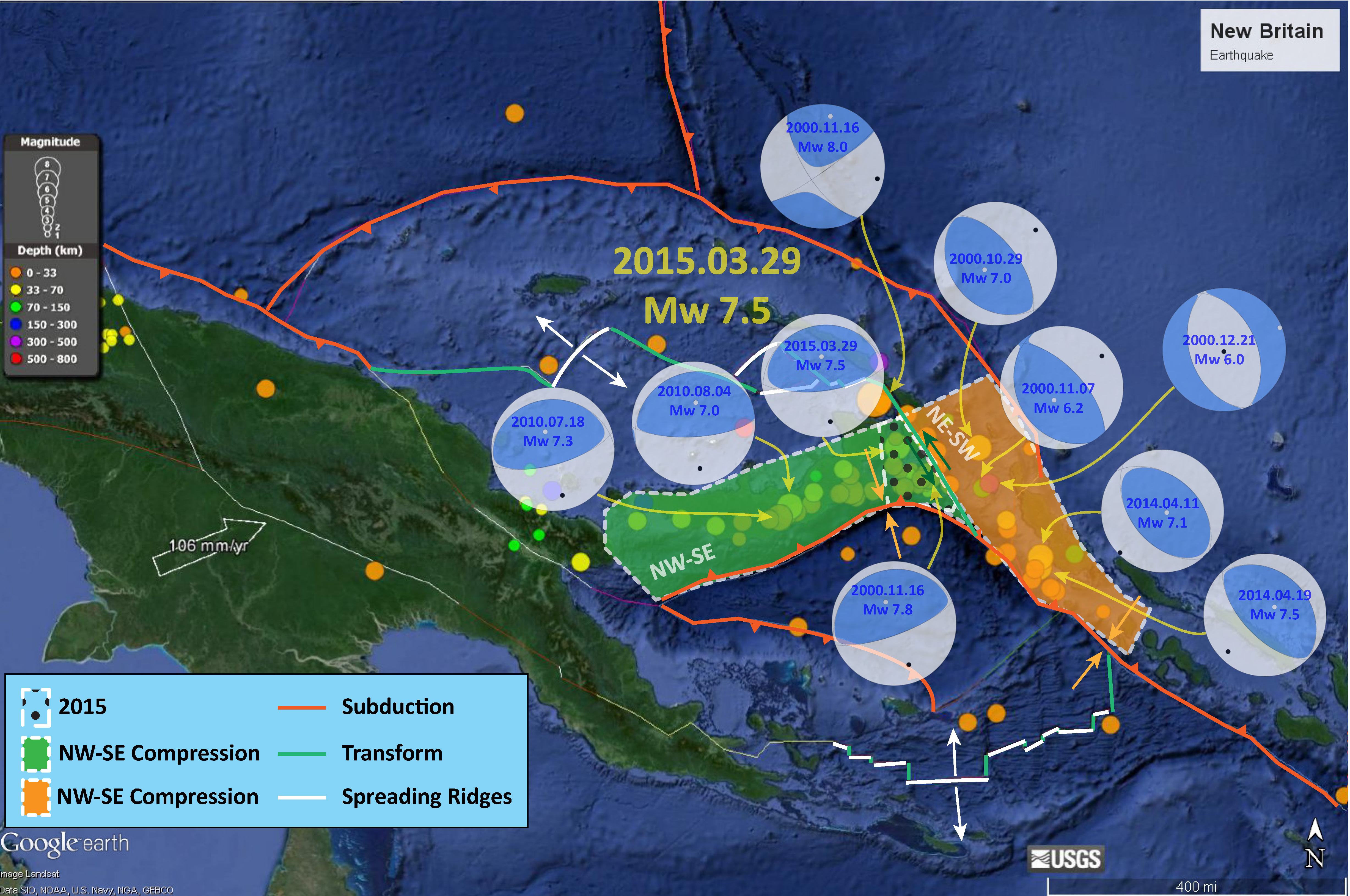
- In earlier earthquake reports, I discussed seismicity from 2000-2015 here. The seismicity on the west of this region appears aligned with north-south shortening along the New Britain trench, while seismicity on the east of this region appears aligned with more east-west shortening. Here is a map that I put together where I show these two tectonic domains with the seismicity from this time period (today’s earthquakes are not plotted on this map, but one may see where they might plot).
- Here is the slab interpretation for the New Britain region from Holm and Richards, 2013. I include the figure caption below as a blockquote.
- Here are the forward models for the slab in the New Britain region from Holm and Richards, 2013. I include the figure caption below as a blockquote.
- Here is a map showing some detailed mapping of the Weitin fault (Lindley, 2006).
- This figure shows details of the regional tectonics (Holm et al., 2016). I include the figure caption below as a blockquote.
- Here is a larger scale map showing lineaments (thin black lines) which represent structures formed at the spreading ridges (Lindley, 2006). These spreading ridges are perpendicular to the Weitin and sister transform faults (like the Sapom fault).
- The interpretive poster above shows the 2007 M 8.1 tsunamigenic subduction zone earthquake. I presented information about this earthquake in a report from 22 Jan. 2017 here. Below are some of the interpretive posters from that report that show excellent examples of subduction zone earthquakes along the San Cristobal trench.
- Here is my interpretive poster from the 12/17 M 7.9 Bougainville Earthquake, possibly (probably) related to today’s M 7.9 earthquake. This is my Earthquake Report for the 12/17 earthquake.
- For a comparison, here is an earthquake that happened along the New Britain subduction zone. Note how the orientation of the earthquake mechanism is aligned with the trench.
- Here is the map with a century’s seismicity plotted.
- Here are the maps from Holm et al. (2019) that show the sources of volcanic rocks in the region.
- This is a series of plate reconstructions from Holm et al. (2019), the final panel is in the interpretive poster above.
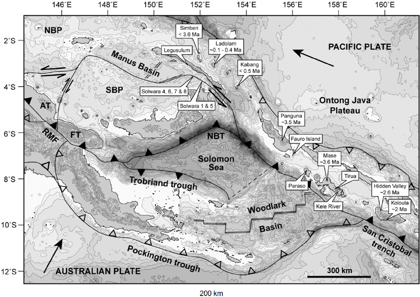
Tectonic setting and mineral deposits of eastern Papua New Guinea and Solomon Islands. The modern arc setting related to formation of the mineral deposits comprises, from west to east, the West Bismarck arc, the New Britain arc, the Tabar-Lihir-Tanga-Feni Chain and the Solomon arc, associated with north-dipping subduction/underthrusting at the Ramu-Markham fault zone, New Britain trench and San Cristobal trench respectively. Arrows denote plate motion direction of the Australian and Pacific plates. Filled triangles denote active subduction. Outlined triangles denote slow or extinct subduction. NBP: North Bismarck plate; SBP: South Bismarck plate; AT: Adelbert Terrane; FT: Finisterre Terrane; RMF: Ramu-Markham fault zone; NBT: New Britain trench.
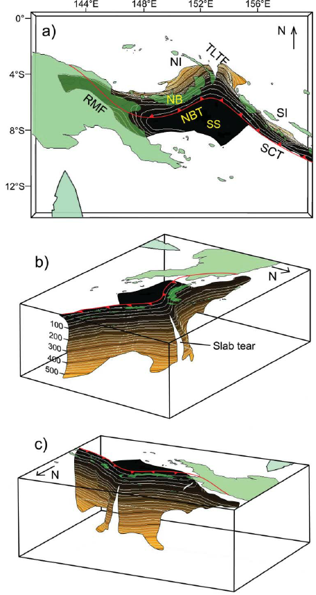
3-D model of the Solomon slab comprising the subducted Solomon Sea plate, and associated crust of the Woodlark Basin and Australian plate subducted at the New Britain and San Cristobal trenches. Depth is in kilometres; the top surface of the slab is contoured at 20 km intervals from the Earth’s surface (black) to termination of slabrelated seismicity at approximately 550 km depth (light brown). Red line indicates the locations of the Ramu-Markham Fault (RMF)–New Britain trench (NBT)–San Cristobal trench (SCT); other major structures are removed for clarity; NB, New Britain; NI, New Ireland; SI, Solomon Islands; SS, Solomon Sea; TLTF, Tabar–Lihir–Tanga–Feni arc. See text for details.
Forward tectonic reconstruction of progressive arc collision and accretion of New Britain to the Papua New Guinea margin. (a) Schematic forward reconstruction of New Britain relative to Papua New Guinea assuming continued northward motion of the Australian plate and clockwise rotation of the South Bismarck plate. (b) Cross-sections illustrate a conceptual interpretation of collision between New Britain and Papua New Guinea.

Weitin Fault, Southern New Ireland, showing trace of fault, topography and evidence used by Hohnen (1978) to tentatively suggest sinistral fault movement (after Hohnen, 1978).
a) Present day tectonic features of the Papua New Guinea and Solomon Islands region as shown in plate reconstructions. Sea floor magnetic anomalies are shown for the Caroline plate (Gaina and Müller, 2007), Solomon Sea plate (Gaina and Müller, 2007) and Coral Sea (Weissel and Watts, 1979). Outline of the reconstructed Solomon Sea slab (SSP) and Vanuatu slab (VS)models are as indicated. b) Cross-sections related to the present day tectonic setting. Section locations are as indicated. Bismarck Sea fault (BSF); Feni Deep (FD); Louisiade Plateau
(LP); Manus Basin (MB); New Britain trench (NBT); North Bismarck microplate (NBP); North Solomon trench (NST); Ontong Java Plateau (OJP); Ramu-Markham fault (RMF); San Cristobal trench (SCT); Solomon Sea plate (SSP); South Bismarck microplate (SBP); Trobriand trough (TT); projected Vanuatu slab (VS); West Bismarck fault (WBF); West Torres Plateau (WTP); Woodlark Basin (WB).

Map showing onshore structures of the Gazelle Peninsula and New Ireland and those interpreted from SeaMARC II sidescan backscatter data in the Eastern Bismarck Sea. BSSL, Bismarck Sea Seismic Lineation (BSSL). SeaMARC II backscatter data from which lineations have been picked are from Taylor et al. (1991 a-c). Modified after Madsen and Lindley (1994).
Here is a visualization of the seismicity as presented by Dr. Steve Hicks.

Tectonic setting of Papua New Guinea and Solomon Islands. A) Regional plate boundaries and tectonic elements. Light grey shading illustrates bathymetry <2000m below sea level indicative of continental or arc crust, and oceanic plateaus. The New Guinea Orogen comprises rocks of the New Guinea Mobile Belt and the Papuan Fold and Thrust Belt; Adelbert Terrane (AT); Aure-Moresby trough (AMT); Bougainville Island (B); Bismarck Sea fault (BSF); Bundi fault zone (BFZ); Choiseul Island (C); Feni Deep (FD); Finisterre Terrane (FT); Guadalcanal Island (G); Gazelle Peninsula (GP); Kia-Kaipito-Korigole fault zone (KKKF); Lagaip fault zone (LFZ); Malaita Island (M); Manus Island (MI); New Britain (NB); New Georgia Islands (NG); New Guinea Mobile Belt (NGMB); New Ireland (NI); Papuan Fold and Thrust Belt (PFTB); Ramu-Markham fault (RMF); Santa Isabel Island (SI); Sepik arc (SA); Weitin Fault (WF); West Bismarck fault (WBF); Willaumez-Manus Rise (WMR). Arrows indicate rate and direction of plate motion of the Australian and Pacific plates (MORVEL, DeMets et al., 2010); B) Pliocene-Quaternary volcanic centres and magmatic arcs related to this study. Figure modified from Holm et al. (2016). Subduction zone symbols with filled pattern denote active subduction; empty symbols denote extinct subduction zone or negligible convergence.
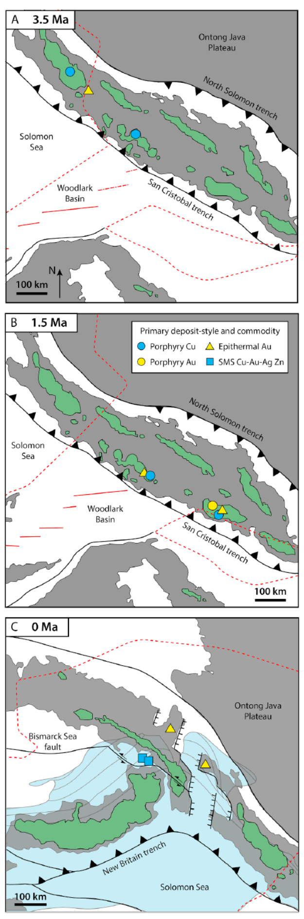
Selected tectonic reconstructions and mineral deposit formation for key areas and times within the eastern Papua New Guinea and Solomon Islands region. A) Formation of the Panguna and Fauro Island Deposits above the interpreted subducted margin of the Solomon Sea plate-Woodlark Basin, and Mase deposit above the subducting Woodlark spreading center; B) Formation of the New Georgia deposits above the subducting Woodlark spreading center, and Guadalcanal deposits above the subducting margin of the Woodlark Basin; C) Formation of the Solwara deposits related to transtension along the Bismarck Sea fault above the subducting Solomon Sea plate, and deposits of the Tabar- Lihir-Tanga-Feni island arc chain related to upper plate extension (normal faulting indicated by hatched linework between New Ireland and Bougainville), while the Ladolam deposit forms above a tear in the subducting slab. Interpreted Solomon Sea slab (light blue shaded area for present-day) is from Holm and Richards (2013); the reconstructed surface extent or indicative trend of slab structure is indicated by the dashed red lines. Green regions denote the present-day landmass using modern coastlines; grey regions are indicative of crustal extent using the 2000m bathymetric contour. The reconstruction is presented here relative to the global moving hotspot reference frame, please see the reconstruction files in the supplementary material for specific reference frames.
Geologic Fundamentals
- For more on the graphical representation of moment tensors and focal mechanisms, check this IRIS video out:
- Here is a fantastic infographic from Frisch et al. (2011). This figure shows some examples of earthquakes in different plate tectonic settings, and what their fault plane solutions are. There is a cross section showing these focal mechanisms for a thrust or reverse earthquake. The upper right corner includes my favorite figure of all time. This shows the first motion (up or down) for each of the four quadrants. This figure also shows how the amplitude of the seismic waves are greatest (generally) in the middle of the quadrant and decrease to zero at the nodal planes (the boundary of each quadrant).

- Here is another way to look at these beach balls.
The two beach balls show the stike-slip fault motions for the M6.4 (left) and M6.0 (right) earthquakes. Helena Buurman's primer on reading those symbols is here. pic.twitter.com/aWrrb8I9tj
— AK Earthquake Center (@AKearthquake) August 15, 2018
- There are three types of earthquakes, strike-slip, compressional (reverse or thrust, depending upon the dip of the fault), and extensional (normal). Here is are some animations of these three types of earthquake faults. The following three animations are from IRIS.
Strike Slip:
Compressional:
Extensional:
- This is an image from the USGS that shows how, when an oceanic plate moves over a hotspot, the volcanoes formed over the hotspot form a series of volcanoes that increase in age in the direction of plate motion. The presumption is that the hotspot is stable and stays in one location. Torsvik et al. (2017) use various methods to evaluate why this is a false presumption for the Hawaii Hotspot.
- Here is a map from Torsvik et al. (2017) that shows the age of volcanic rocks at different locations along the Hawaii-Emperor Seamount Chain.
- Here is a great tweet that discusses the different parts of a seismogram and how the internal structures of the Earth help control seismic waves as they propagate in the Earth.

A cutaway view along the Hawaiian island chain showing the inferred mantle plume that has fed the Hawaiian hot spot on the overriding Pacific Plate. The geologic ages of the oldest volcano on each island (Ma = millions of years ago) are progressively older to the northwest, consistent with the hot spot model for the origin of the Hawaiian Ridge-Emperor Seamount Chain. (Modified from image of Joel E. Robinson, USGS, in “This Dynamic Planet” map of Simkin and others, 2006.)

Hawaiian-Emperor Chain. White dots are the locations of radiometrically dated seamounts, atolls and islands, based on compilations of Doubrovine et al. and O’Connor et al. Features encircled with larger white circles are discussed in the text and Fig. 2. Marine gravity anomaly map is from Sandwell and Smith.
Today, on #SeismogramSaturday: what are all those strangely-named seismic phases described in seismograms from distant earthquakes? And what do they tell us about Earth’s interior? pic.twitter.com/VJ9pXJFdCy
— Jackie Caplan-Auerbach (@geophysichick) February 23, 2019
- 2019.05.14 M 7.5 New Ireland
- 2019.05.06 M 7.2 Papua New Guinea
- 2018.12.05 M 7.5 New Caledonia
- 2018.10.10 M 7.0 New Britain, PNG
- 2018.09.09 M 6.9 Kermadec
- 2018.08.29 M 7.1 Loyalty Islands
- 2018.08.18 M 8.2 Fiji
- 2018.03.26 M 6.9 New Britain
- 2018.03.26 M 6.6 New Britain
- 2018.03.08 M 6.8 New Ireland
- 2018.02.25 M 7.5 Papua New Guinea
- 2018.02.26 M 7.5 Papua New Guinea Update #1
- 2017.11.19 M 7.0 Loyalty Islands Update #1
- 2017.11.07 M 6.5 Papua New Guinea
- 2017.11.04 M 6.8 Tonga
- 2017.10.31 M 6.8 Loyalty Islands
- 2017.08.27 M 6.4 N. Bismarck plate
- 2017.05.09 M 6.8 Vanuatu
- 2017.03.19 M 6.0 Solomon Islands
- 2017.03.05 M 6.5 New Britain
- 2017.01.22 M 7.9 Bougainville
- 2017.01.03 M 6.9 Fiji
- 2016.12.17 M 7.9 Bougainville
- 2016.12.08 M 7.8 Solomons
- 2016.10.17 M 6.9 New Britain
- 2016.10.15 M 6.4 South Bismarck Sea
- 2016.09.14 M 6.0 Solomon Islands
- 2016.08.31 M 6.7 New Britain
- 2016.08.12 M 7.2 New Hebrides Update #2
- 2016.08.12 M 7.2 New Hebrides Update #1
- 2016.08.12 M 7.2 New Hebrides
- 2016.04.06 M 6.9 Vanuatu Update #1
- 2016.04.03 M 6.9 Vanuatu
- 2015.03.30 M 7.5 New Britain (Update #5)
- 2015.03.30 M 7.5 New Britain (Update #4)
- 2015.03.29 M 7.5 New Britain (Update #3)
- 2015.03.29 M 7.5 New Britain (Update #2)
- 2015.03.29 M 7.5 New Britain (Update #1)
- 2015.03.29 M 7.5 New Britain
- 2015.11.18 M 6.8 Solomon Islands
- 2015.05.24 M 6.8, 6.8, 6.9 Santa Cruz Islands
- 2015.05.05 M 7.5 New Britain
New Britain | Solomon | Bougainville | New Hebrides | Tonga | Kermadec Earthquake Reports
General Overview
Earthquake Reports
Social Media
- Baldwin, S.L., Monteleone, B.D., Webb, L.E., Fitzgerald, P.G., Grove, M., and Hill, E.J., 2004. Pliocene eclogite exhumation at plate tectonic rates in eastern Papua New Guinea in Nature, v. 431, p/ 263-267, doi:10.1038/nature02846.
- Baldwin, S.L., Fitzgerald, P.G., and Webb, L.E., 2012. Tectonics of the New Guinea Region, Annu. Rev. Earth Planet. Sci., v. 40, pp. 495-520.
- Cloos, M., Sapiie, B., Quarles van Ufford, A., Weiland, R.J., Warren, P.Q., and McMahon, T.P., 2005, Collisional delamination in New Guinea: The geotectonics of subducting slab breakoff: Geological Society of America Special Paper 400, 51 p., doi: 10.1130/2005.2400.
- Hamilton, W.B., 1979. Tectonics of the Indonesian Region, USGS Professional Paper 1078.
- Frisch, W., Meschede, M., Blakey, R., 2011. Plate Tectonics, Springer-Verlag, London, 213 pp.
- Geist, E. L., and T. Parsons (2005), Triggering of tsunamigenic aftershocks from large strike-slip earthquakes: Analysis of the November 2000 New Ireland earthquake sequence, Geochem. Geophys. Geosyst., 6, Q10005, https://doi.org/10.1029/2005GC000935.
- Hayes, G., 2018, Slab2 – A Comprehensive Subduction Zone Geometry Model: U.S. Geological Survey data release, https://doi.org/10.5066/F7PV6JNV.
- Highland, L.M., and Bobrowsky, P., 2008. The landslide handbook—A guide to understanding landslides, Reston, Virginia, U.S. Geological Survey Circular 1325, 129 p.
- Holm, R. and Richards, S.W., 2013. A re-evaluation of arc-continent collision and along-arc variation in the Bismarck Sea region, Papua New Guinea in Australian Journal of Earth Sciences, v. 60, p. 605-619.
- Holm, R.J., Richards, S.W., Rosenbaum, G., and Spandler, C., 2015. Disparate Tectonic Settings for Mineralisation in an Active Arc, Eastern Papua New Guinea and the Solomon Islands in proceedings from PACRIM 2015 Congress, Hong Kong ,18-21 March, 2015, pp. 7.
- Holm, R.J., Rosenbaum, G., Richards, S.W., 2016. Post 8 Ma reconstruction of Papua New Guinea and Solomon Islands: Microplate tectonics in a convergent plate boundary setting in Eartth Science Reviews, v. 156, p. 66-81.
- Holm, R.J., Tapster, S., Jelsma, H.A., Rosenbaum, G., and Mark, D.F., 2019. Tectonic evolution and copper-gold metallogenesis of the Papua New Guinea and Solomon Islands region in Ore Geology Reviews, v. 104, p. 208-226, https://doi.org/10.1016/j.oregeorev.2018.11.007
- Jessee, M.A.N., Hamburger, M. W., Allstadt, K., Wald, D. J., Robeson, S. M., Tanyas, H., et al. (2018). A global empirical model for near-real-time assessment of seismically induced landslides. Journal of Geophysical Research: Earth Surface, 123, 1835–1859. https://doi.org/10.1029/2017JF004494
- Johnson, R.W., 1976, Late Cainozoic volcanism and plate tectonics at the southern margin of the Bismarck Sea, Papua New Guinea, in Johnson, R.W., ed., 1976, Volcanism in Australia: Amsterdam, Elsevier, p. 101-116
- Keefer, D.K., 1984. Landslides Caused by Earthquakes in GSA Bulletin, v. 95, p. 406-421
- Kreemer, C., G. Blewitt, E.C. Klein, 2014. A geodetic plate motion and Global Strain Rate Model in Geochemistry, Geophysics, Geosystems, v. 15, p. 3849-3889, https://doi.org/10.1002/2014GC005407.
- Lindley, I.D., 2006. Extensional and vertical tectonics in the New Guinea islands: implications for island arc evolution in Annals of Geophysics, suppl to v. 49, no. 1, p. 403-426
- Meyer, B., Saltus, R., Chulliat, a., 2017. EMAG2: Earth Magnetic Anomaly Grid (2-arc-minute resolution) Version 3. National Centers for Environmental Information, NOAA. Model. https://doi.org/10.7289/V5H70CVX
- Müller, R.D., Sdrolias, M., Gaina, C. and Roest, W.R., 2008, Age spreading rates and spreading asymmetry of the world’s ocean crust in Geochemistry, Geophysics, Geosystems, 9, Q04006, https://doi.org/10.1029/2007GC001743
- Tregoning, P., Jackong, R.J., McQueen, H., Lambeck, K., Stevens, C., Little, R.P., Curley, R., and Rosa, R., 1999. Motion of the South Bismarck Plate, Papua New Guinea in GRL, v. 26, no. 23, p. 3517-3520
- Tregoning, P., McQueen, H., Lambeck, K., Jackson, R. Little, T., Saunders, S., and Rosa, R., 2000. Present-day crustal motion in Papua New Guinea, Earth Planets and Space, v. 52, pp. 727-730.
- Tregoning, P., Sambridge, M., McQueen, H., Toulin, S., and Nicholson, T., 2005. Motion of the South Bismarck Plate, Papua New Guinea in GJI, v. 160, p. 1103-111, https://doi.org/10.111/j.1365-246X.2005.02567.x
- USGS, 2004. Landslide Types and Processes, U.S. Geological Survey Fact Sheet 2004-3072
- Zhu, J., Baise, L. G., Thompson, E. M., 2017, An Updated Geospatial Liquefaction Model for Global Application, Bulletin of the Seismological Society of America, 107, p 1365-1385, doi: 0.1785/0120160198
References:
Return to the Earthquake Reports page.