Initial Narrative
Well, it has been a very busy week. I had gotten back from the American Geophysical Union Fall Meeting in Chicago late Saturday night. I had one day to hang out with my cats before I was to head down to Santa Cruz to meet with the city there to discuss installing a tide gage. Santa Cruz lacks a gage yet receives large tsunami inundations.
So, I drove down and got there about 10pm Monday evening. I was up for an hour or two and went to sleep.
At shortly after 2:30am I got a text message about a M 6.4 earthquake near Ferndale. I immediately got up and texted my colleague Cynthia Pridmore. We are tasked to prepare Earthquake Quick Reports that we (California Geological Survey, CGS) provide to the California Governor’s Office of Emergency Services (Cal OES). These reports provide technical information that helps them provide resources to local first responders during times following natural hazards impacts.
https://earthquake.usgs.gov/earthquakes/eventpage/nc73821036/executive
These reports are reviewed by the head of the Seismic Hazards Program (Tim Dawson) and by the State Geologist prior to being provided to the leadership in our organization and parent organizations. Reports for larger earthquakes and tsunami sometimes end up on the Governor’s desk.
We got our report submitted within about 45 minutes and we prepared for a long couple of days. We at CGS met at 8am to discuss our field response activities.
CGS and the U.S. Geological Survey (USGS) work closely together to document field evidence from earthquakes and tsunami. Kate Thomas (CGS) and Luke Blair (USGS) have a database ready to go within about 15 minutes after an earthquake. This database is used on mobile devices to collect observational information that include photos and other information. We use the ESRI Field Maps app for this purpose.
We decided to send CGS staff from the Eureka office out to collect information. I was to drive back to Humboldt and then join the field teams the following day.
Something that also happens following significant or damaging earthquakes is the activation of the California Earthquake Clearinghouse. Pridmore (CGS) is the chair of the EQCH and works with our partners (USGS, EERI, etc.) to decide when to activate the EQCH.
Data from these CGS/USGS field observations, along with data from other field teams, are posted onto the EQCH page for this event. Here is where those data are made available for this M 6.4 Ferndale Earthquake. The dataset of field observations are posted on that page are found by clicking on the “Resources” tab, also linked here.
When I returned to my home, the power was still out. We (CGS) had a scheduled meeting at 6pm and the EQCH meeting at 7pm. So, I went to the Eureka National Weather Service (NWS) Office on Woodley Island. They have electric power backup and satellite internet access. I work closely with the NWS and Cal OES and have been granted access to set up my workstation there during natural hazard emergencies like earthquake and tsunami. This was we can all better coordinate our actions without the burden of having power or internet outages at our residences. We are thankful for these relationships between CGS, the NWS (Ryan Aylward, Troy Nicolini) and Cal OES Eureka (Todd Becker).
So, I got up very early to work with my co-workers to continue the field investigations. There was little geological evidence from the earthquake. We identified some landslides and cracks in road fill. We did not locate any evidence for liquefaction, even though the USGS liquefaction susceptibility data suggested a high chance for that phenomena.
The Earthquake Report
This earthquake is in a tectonically complicated region of the western United States, the Mendocino triple junction. Here, three plate boundary fault systems meet (the definition of a triple junction): the San Andreas fault from the south, the Cascadia subduction zone from the north, and the Mendocino fault from the west. These plate boundary fault systems all overlap like fingers do when we fold our hands together.
The Cascadia subduction zone is a convergent (moving together) plate boundary where the Gorda and Juan de Fuca plates dive into the Earth beneath the North America plate. The fault formed here is called the megathrust subduction zone fault. Earthquakes on subduction zone faults generate the largest magnitude earthquakes of all fault types and also generate tsunami that can impact the local area and also travel across the ocean to impact places elsewhere. The most recent known Cascadia megathrust subduction zone fault earthquake was in January 1700.
The San Andreas and Mendocino fault systems are strike-slip (plates move side by side) fault systems. Many are familiar with the 1906 San Francisco Earthquake.
While the largest source of annual seismicity are intraplate Gorda plate earthquakes, the two largest contributors to seismic hazards in California are the Cascadia subduction zone (CSZ) and the San Andreas fault (SAF) systems. These sources overlap in the region of the Mendocino triple junction (MTJ) and may interact in ways we are only beginning to understand as evidenced by the 2016 M7.8 Kaikōura earthquake in New Zealand (Clark et al., 2017 Litchfield et al., 2018), which occurred along a similar subduction/transform boundary, and included co-seismic rupture of more than 20 faults.
The M 6.4 earthquake was a strike-slip earthquake within the downgoing Gorda plate (an intra plate earthquake). The earthquake started offshore and then the fault slipped to the east.
There is modest evidence that this earthquake generated focused seismic waves in the direction of fault slip (this is called directivity). In addition, the area of the lower Eel River Valley is a sedimentary basin. Sedimentary basins are known for amplifying ground shaking and trapping seismic waves, further increasing the ground shaking. The lower Eel River Valley is formed by tectonic folding caused by the northward migration of the Mendocino triple junction (read my contributions in the 2022 Pacific Cell Friends of the Pleistocene guidebook for more information about the structure of the Eel River and Van Duzen River valleys and surrounding regions.
So the seismic waves could have been trapped in the sedimentary basin formed within the Eel River Valley. However, there is an even older sedimentary basin here in which the Eel/Van Duzen river sediments are deposited within. These older sedimentary rocks have different seismic velocity properties that could also affect how seismic waves are transmitted here. There is a terrane bounding fault that separates these older rocks (Cretaceous Franciscan Formation) to the south from the younger rocks (Quaternary-Tertiary Wildcat Group) to the north.
Also, any of the large crustal fault systems (e.g., the Russ fault, the Little Salmon or Table Bluff faults, etc.) could guide seismic waves (a.k.a. act as wave guides), directing them in orientations relative to the fault systems.
My leading hypothesis is that the younger (latest Pleistocene to Holocene) river sediments that form the younger sedimentary basin and the crustal faults are both responsible for modifying the seismic wave transmission from this earthquake.
One thing people almost always ask is about whether or not there is a higher chance that there will be a Cascadia subduction zone earthquake. This is currently impossible to tell. However, we can make some estimates of how forces within the Earth might have changed after a given earthquake. There was a Gorda plate earthquake sequence in 2018 that allowed us to consider these changes in the crust to see if the megathrust was brought more close to rupture. Here is the report from that Gorda plate earthquake sequence.
I will update this report further in the future, as we collect additional information.
One last thing for now. Bob McPherson formed a research group that we call Team Gorda. Team Gorda, supported by Connie Stewart at Cal Poly Humboldt, is using recently constructed fiber cables as a seismic instrument (called distributed acoustic seismic, DAS) to learn more about the underlying tectonic structures in the region. This fiber cable acts as thousands of little seismometers. Jeff McGuire and his team just installed the interrogator in our office at the Arcata City Hall. Horst from the Berkeley Seismic Lab is also working with Bob to install seismometers along the fiber cable so that we can calibrate the DAS observations.
We ran our first DAS experiment earlier this year and plan on doing more experiments far into the future, including fiber cables that are installed from here into the Pacific Ocean (on their way to Asia).
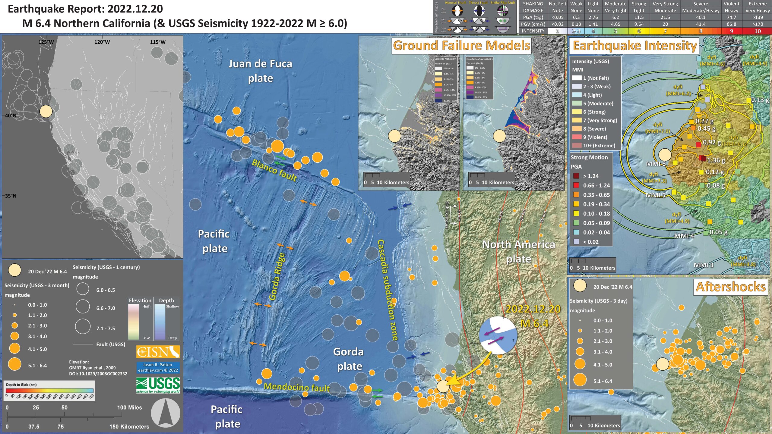
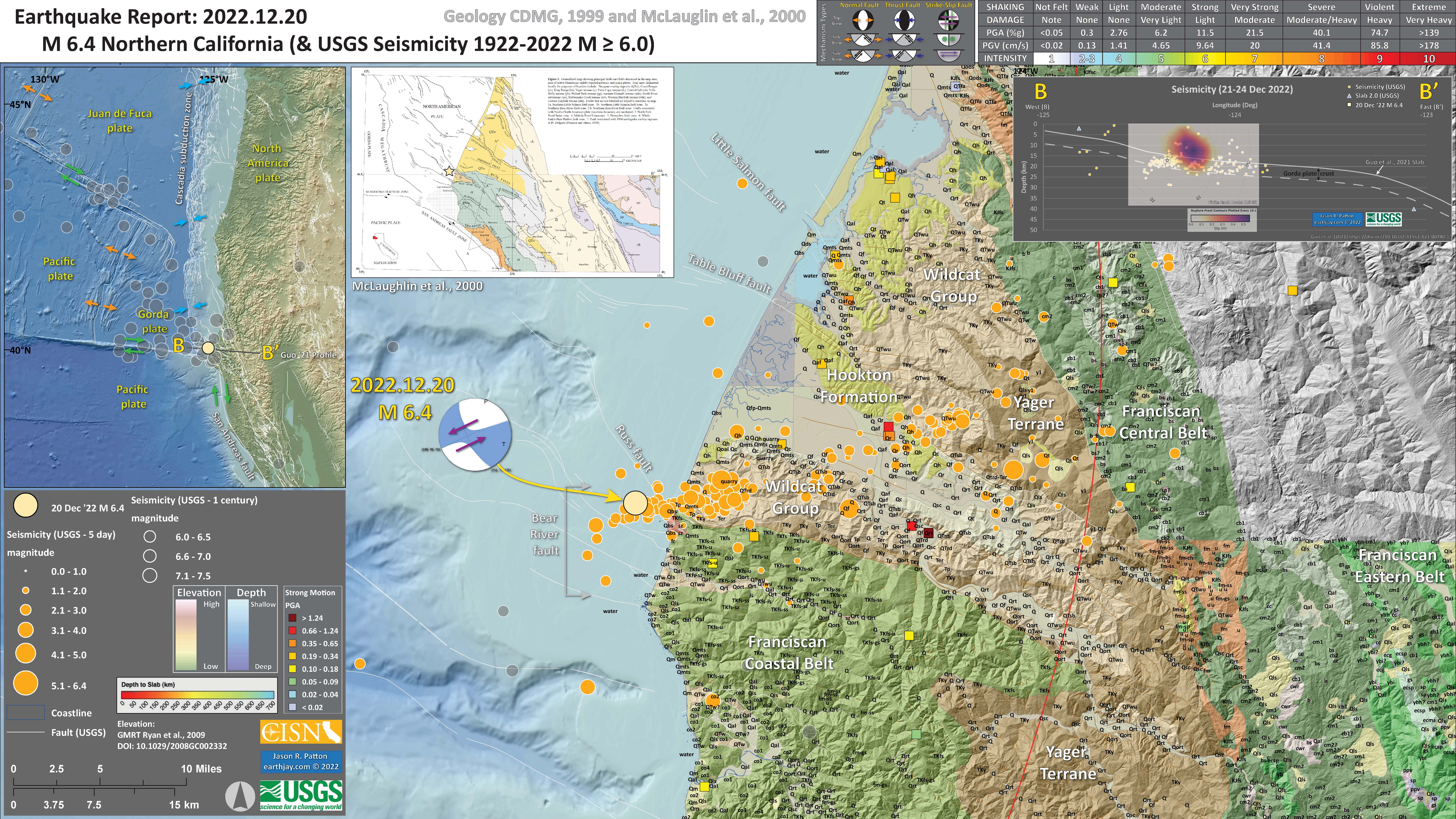
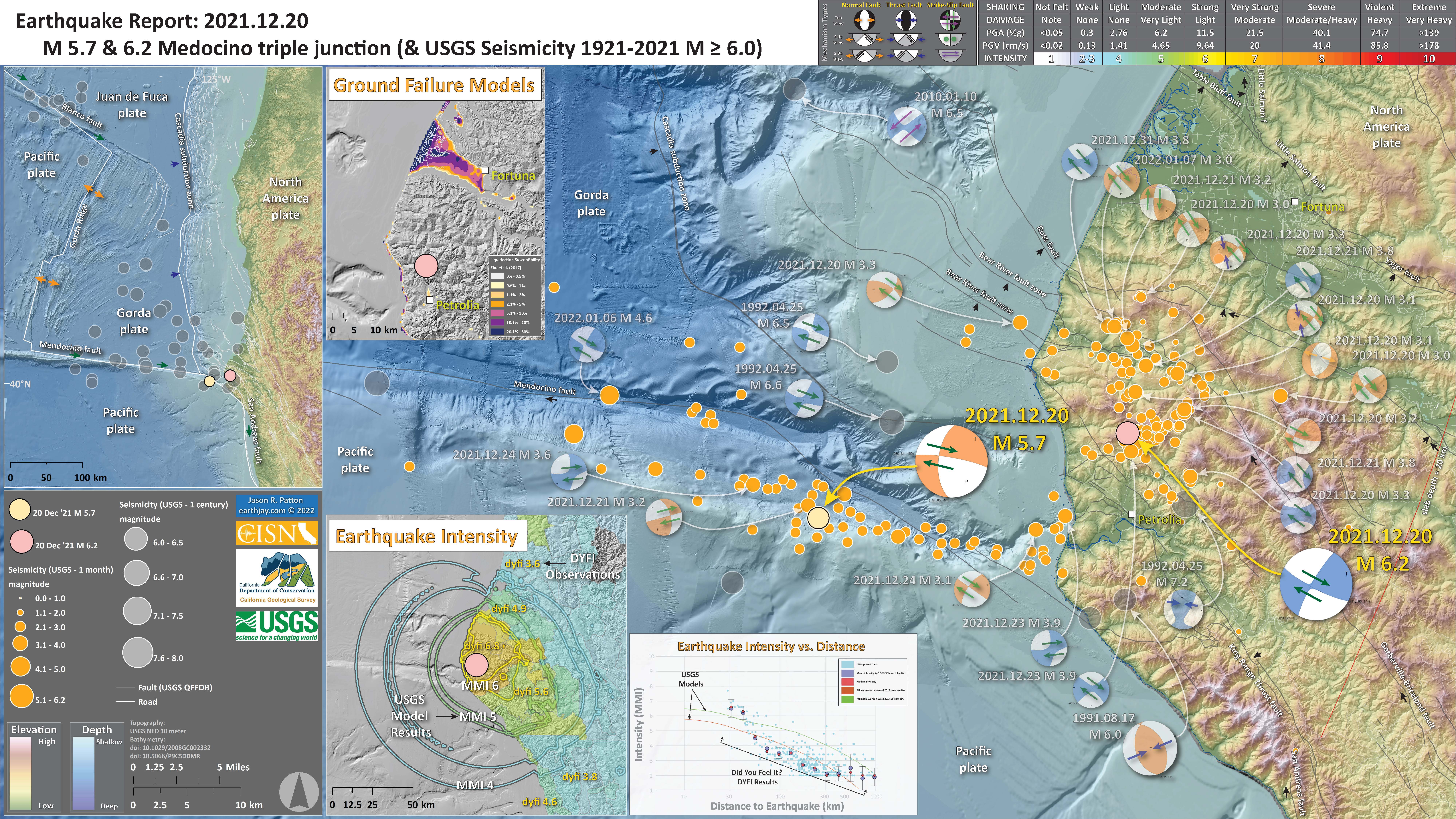
Below is my interpretive poster for this earthquake
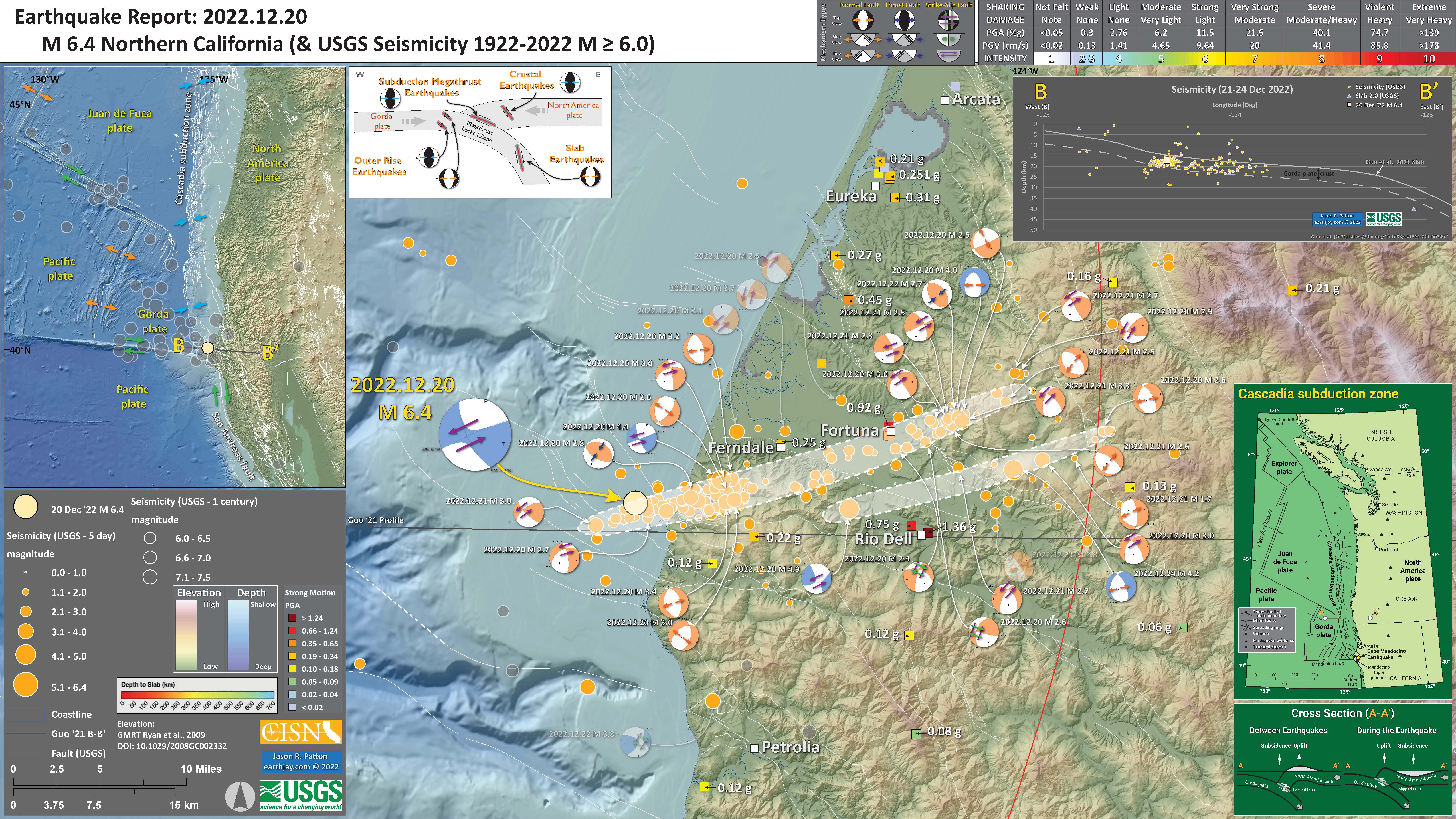
- I plot the seismicity from the past month, with diameter representing magnitude (see legend). I include earthquake epicenters from 1922-2022 with magnitudes M ≥ 3.0 in one version.
- I plot the USGS fault plane solutions (moment tensors in blue and focal mechanisms in orange), possibly in addition to some relevant historic earthquakes.
- A review of the basic base map variations and data that I use for the interpretive posters can be found on the Earthquake Reports page. I have improved these posters over time and some of this background information applies to the older posters.
- Some basic fundamentals of earthquake geology and plate tectonics can be found on the Earthquake Plate Tectonic Fundamentals page.
- In the upper left corner is a map showing the western US and a century of seismicity.
- In the upper right corner is a map that displays a variety of earthquake intensity information. I plot the USGS modeled intensity, the USGS Did You Feel It? observations of intensity, and the shaking magnitude using the Peak Ground Acceleration scale in units of g (gravitational acceleration). I describe this map later in the report.
- To the left of the intensity map are two maps that show the probability (the chance of) earthquake triggered landslides and the susceptibility (the chance of) earthquake induced liquefaction. I will discuss these ground failure models later in the report.
- In the lower right corner I include a plot of aftershocks from a three day period.
I include some inset figures. Some of the same figures are located in different places on the larger scale map below.
- Here is the map with 3 month’s seismicity plotted.

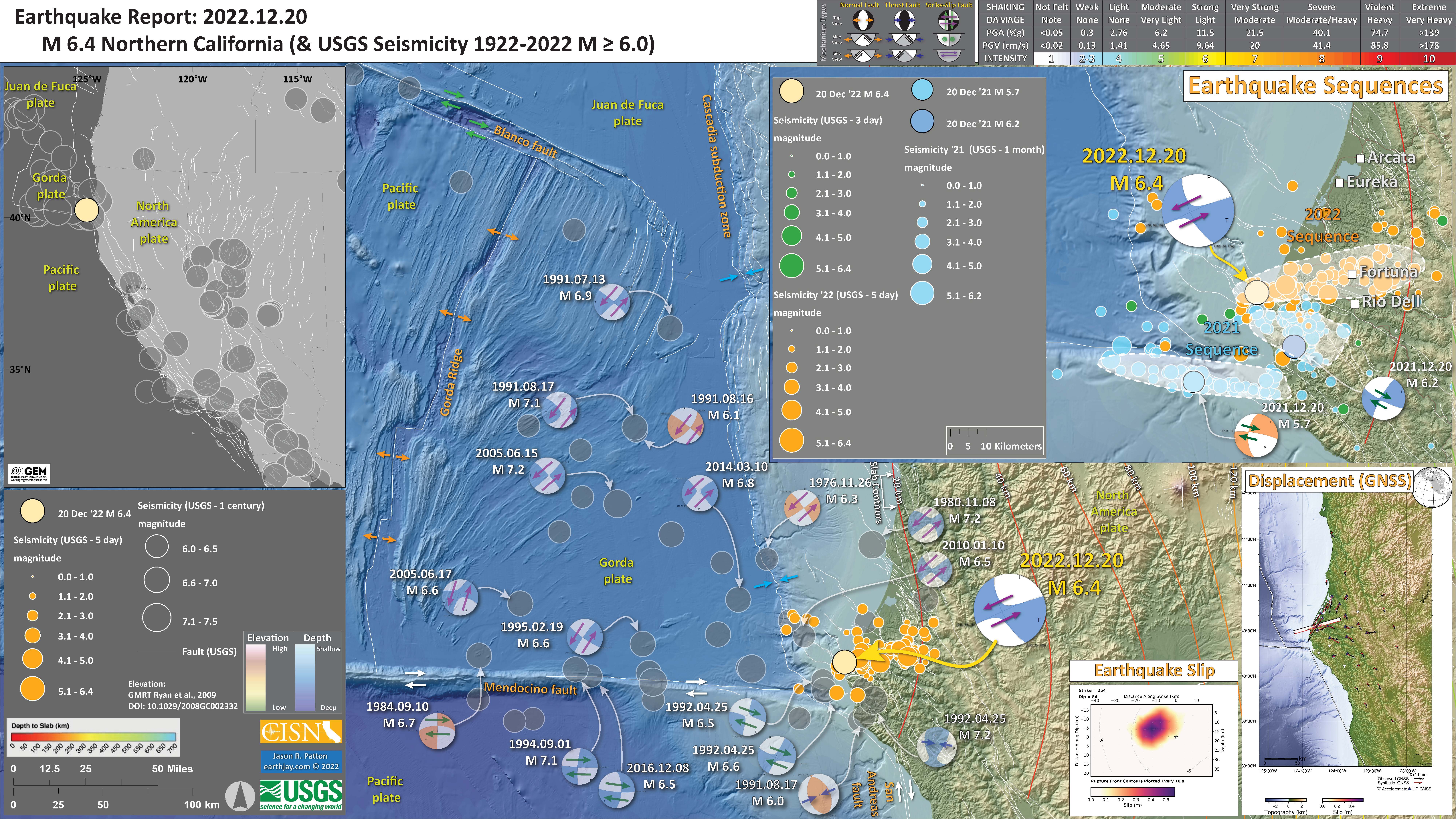
- Here is an updated interpretive poster with 3 day’s seismicity plotted. I describe how this poster is different
- In the lower right corner is a map from the USGS. This map shows where they interpret the location for the causative fault for this earthquake. There are also arrows (vectors) that show how Global Navigation Satellite System (GNSS, used to be called GPS) sites moved during the earthquake and how the moved using a computer simulation of the Earth that incorporate a fault that slipped like shown on the map. These arrows show the direction of motion and the amount of motion.
- To the left of this map is the USGS finite fault model for this earthquake. The colors represent the amount that the fault slipped during the earthquake. This is the fault model that they used to estimate how the GNSS sites moved in the map to the right.
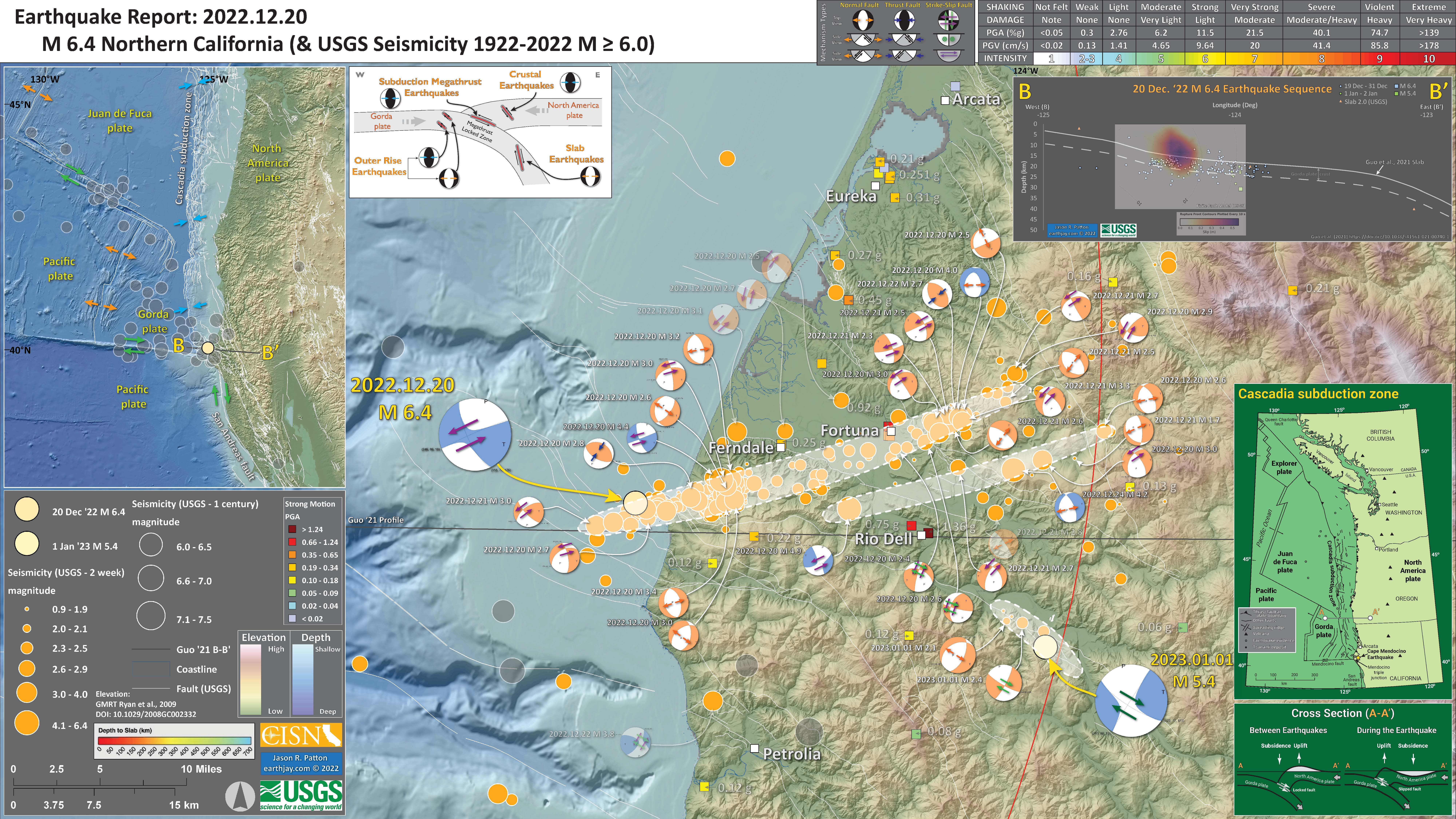
- In the upper right corner is a map that shows the seismicty from the past week (in orange) and seismicity associated with the earthquake sequence from exactly one year before (in blue).
- In the main part of the map I plot the earthquake mechanisms from the past century.
- I felt the M 4.1 earthquake this morning (24 Dec 2022). It was an extensional earthquake in the eastern part of the aftershock region.
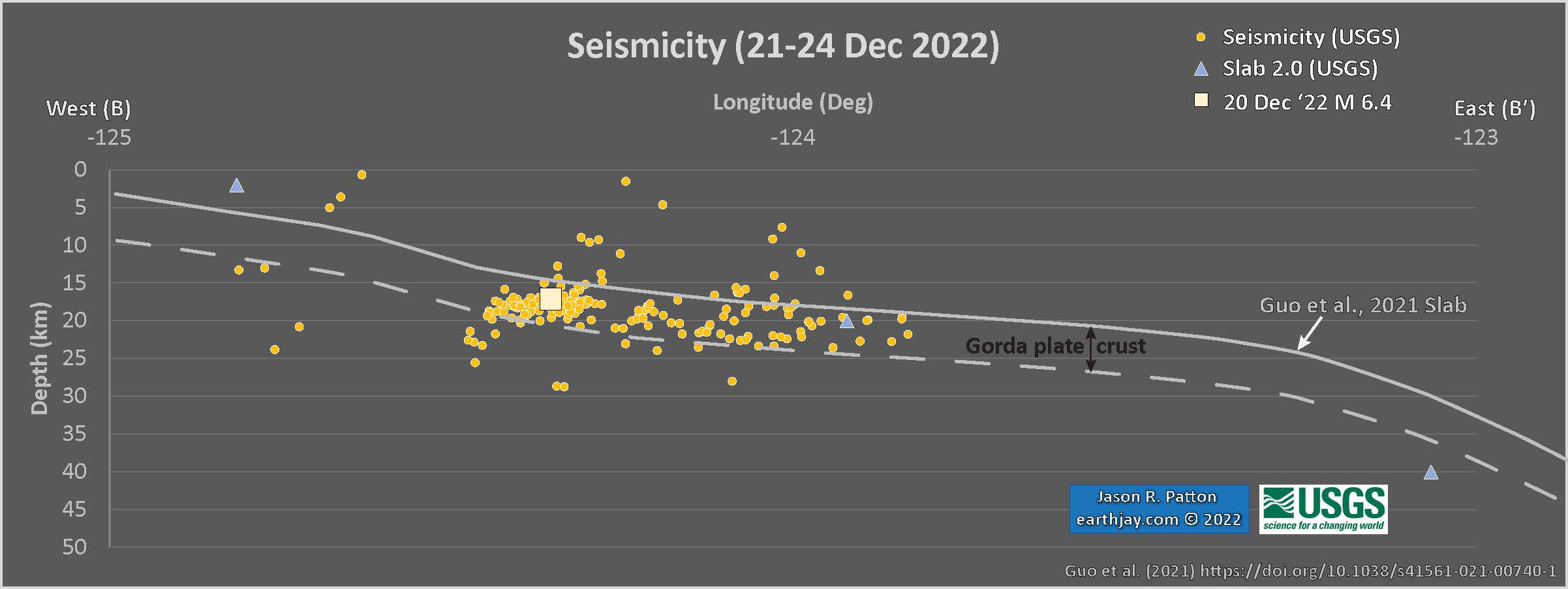
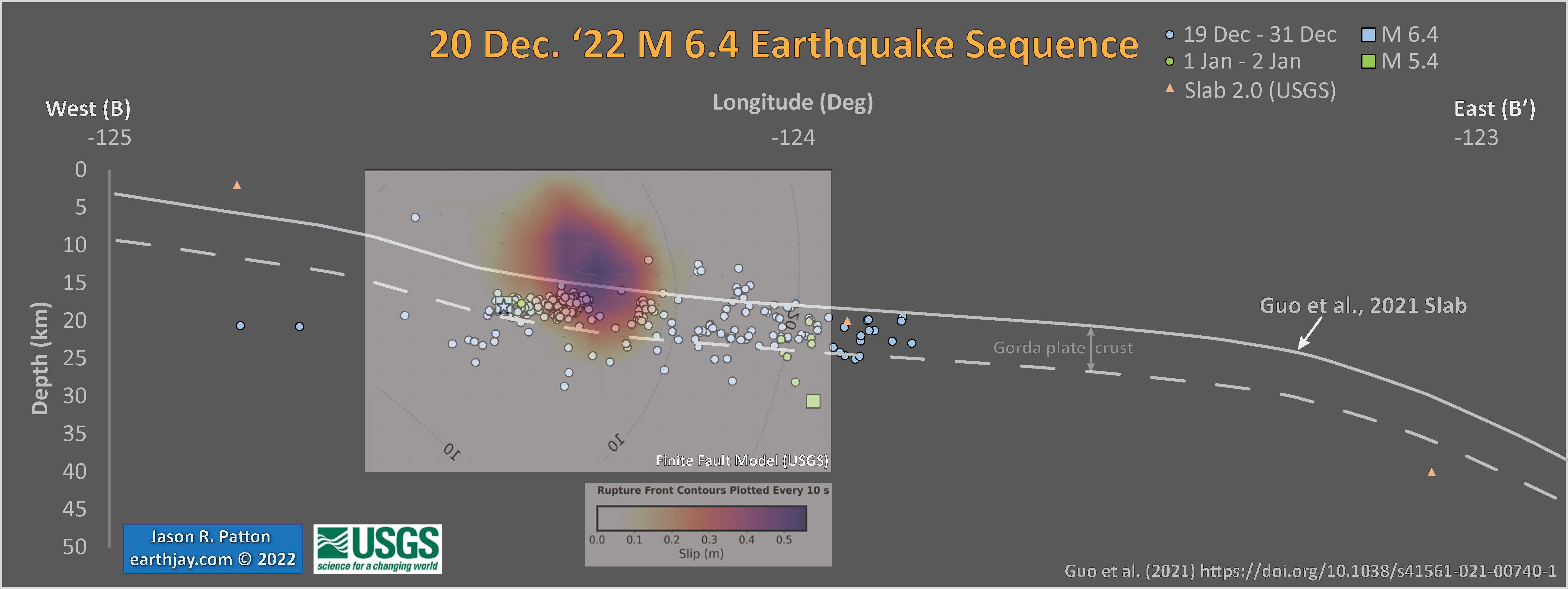
- Today I plotted the seismicity along an east-west profile.
- I traced the Gorda plate geometry from Guo et al. (2018). This is from their profile B-B’ which is just about at 41 degrees north.
- We can see that the mainshock (the M 6.4) and most of the aftershocks are within the Gorda plate.
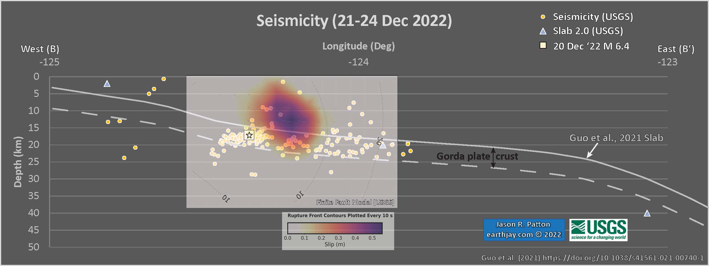
- Here is an updated plot that includes the USGS Finite Fault Model as a transparent overlay.
- Note how most of the slip is in the North America plate.
- Here is an updated plot that displays M 6.4 in blue and M 5.4 in green.
- And if someone wants to learn more about what a hypocenter is, here you go >>>
Seismicity Profile
What is an earthquake? What causes earthquakes and where do they happen? How are earthquakes recorded and measured? Learn more about 'The Science of Earthquakes' at: https://t.co/JAQv4cc2KC pic.twitter.com/pJ2IfQ76bs
— USGS Earthquakes (@USGS_Quakes) January 4, 2023
- Yesterday I got to feel one of the aftershocks, an M 4.2 to the southeast of the main sequence.
- Today I plotted all the aftershocks to date as of this morning. It appears that there were two main faults involved. One about 45 km long and another one about 25 km long.
- I include earthquake mechanisms for all events that I could download today. I placed some mechanisms that may not be related to these 2 faults at 50% transparency.
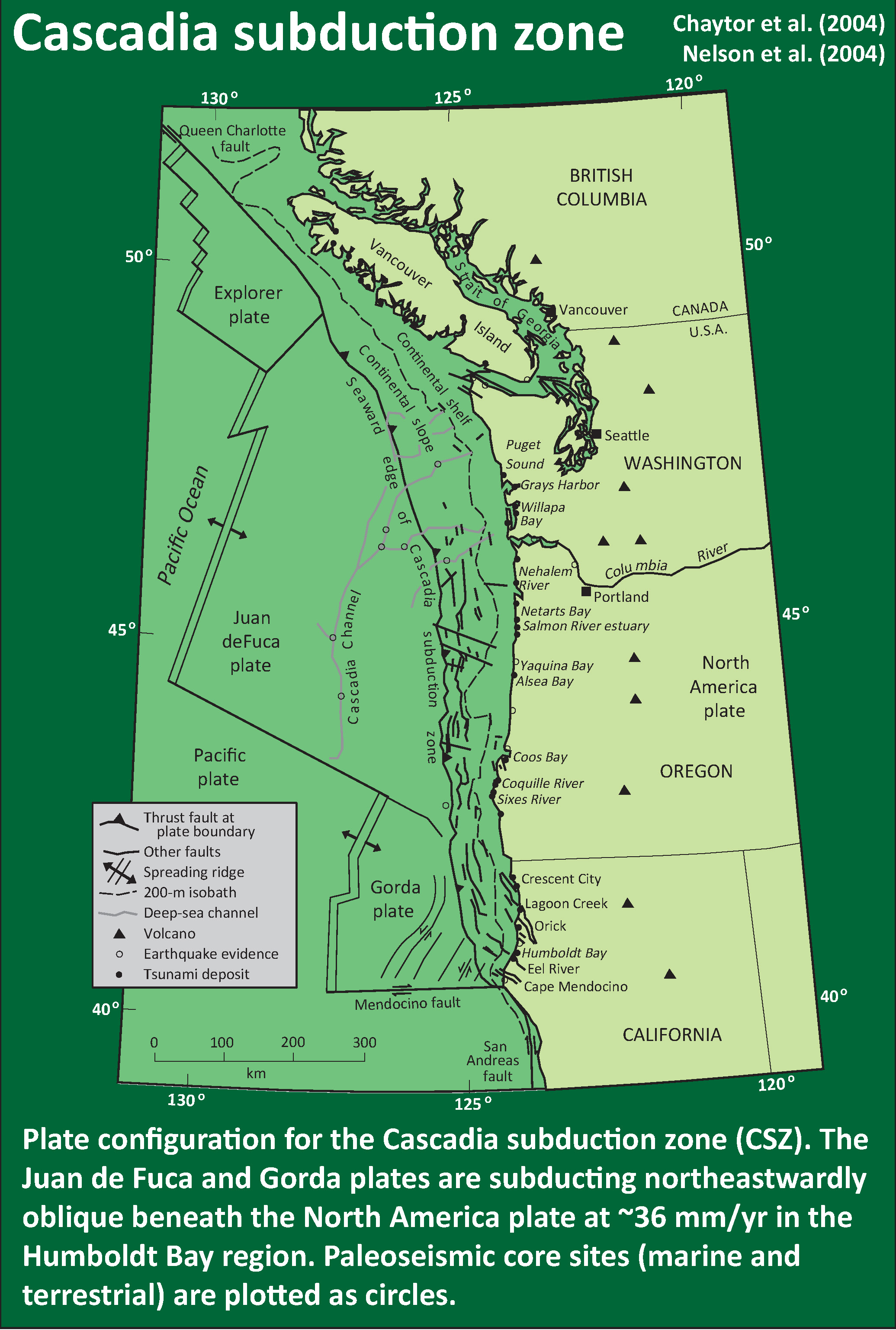
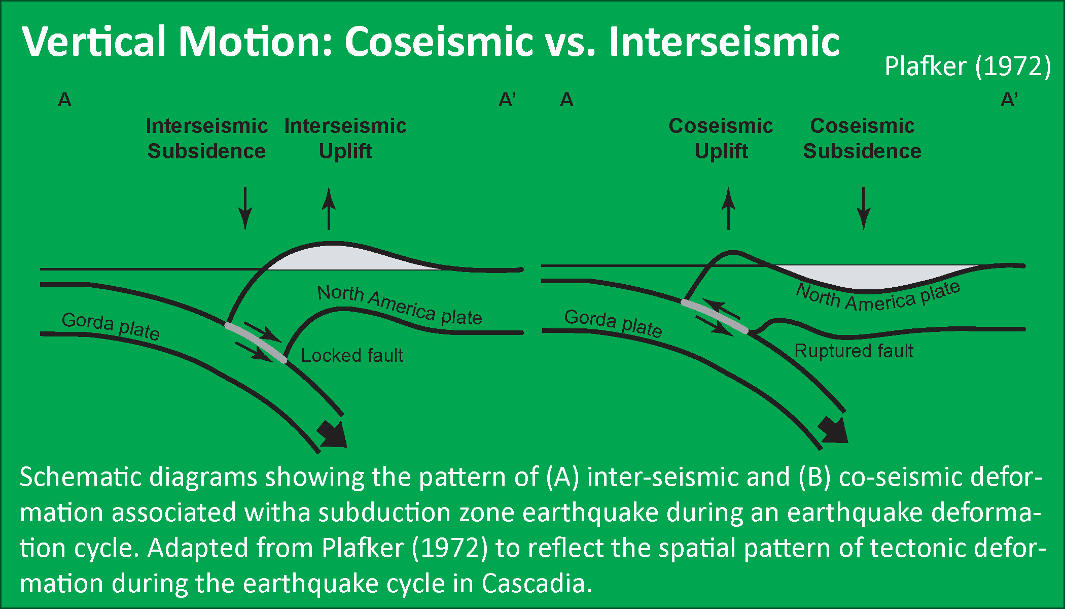
- This poster below includes a map (lower right corner) of the Cascadia subduction zone and the cross section showing how the crust deforms between (interseismic) and during (coseismic) earthquakes.
- I also include a schematic showing where earthquakes might happen (upper left center). Earthquakes along the megathrust subduction zone fault are called interplate earthquakes (like the interstate highways connect between states).
- Earthquakes within the Gorda or North America plates are called intraplate earthquakes. The M 6.4 was an intraplate earthquake within the Gorda plate. I don’t really have a good way to show intraplate strike-slip faults in this diagram (room for future work!).
- In the upper right corner is the seismicity profile that I also show above in the report. When comparing the seismicity with the Guo et al. (2021) slab model, it appears that most of the earthquakes are within the Gorda crust. There are some above, possibly in the North America crust.
- Here is another updated map, updated on 2 January 2023 to include the M 5.4 related earthquakes.
- Now it appears that there are three main faults involved, at least.
- Yesterday I was chatting with Bob McPherson as we were looking at the USGS finite fault slip model. Bob suggested that this model shows that the earthquake slipped in the Gorda and North America plates. If the slip model is correct, then Bob is correct. This is quite interesting if true.
- UPDATE comment (4 jan ’23): I have seen other slip models that do not place M 6.4 slip above the Gorda plate. We must remember that these slip models are non unique solutions and that there is quite a bit of wiggle room for their solutions. Basically, there are knobs to turn on these models (allowing one to change parameters, such as the material properties of the Earth (e.g., the “rheology” of the crust or mantle)) and changing these parameters can change the results while still keeping a good fit to the observational data. It is not uncommon that the slip models for both nodal planes (the two possible fault planes shown on earthquake mechanisms (focal mechanisms or moment tensors)) each fit the data equally well. I have seen the fault model that was fit to the incorrect (incorrect relative to aftershocks) fault plane being chosen as the preferred slip model. So, we must remember this when we are interpreting model results like these fault slip models.
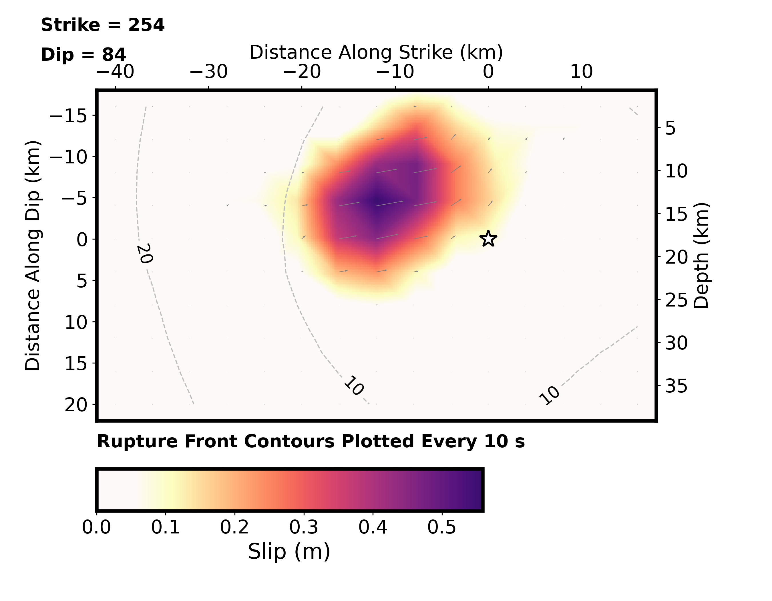
- First lets just look at the finite fault slip model. Below we see a plot with color representing how much the fault slipped. The white star is the M 6.4 hypocenter (the 3-D location of the M 6.4). East is to the left and west is to the left (pretend you are looking at the diagram from the north side of the fault).
- There are gray lines that represent times (10 seconds and 20 seconds after the M 6.4 mainshock) where the rupture propagation front was. So, the fault started slipping at the white star. Then, the fault moved and the outer limit of this motion radiated outwards and was at the first gray line in 10 seconds and at the second gray line at 20 seconds.
- There are small gray arrows that show the direction and magnitude of slip motion along the fault. If we combine this plot with our knowledge that this was a left-lateral strike-slip earthquake, and we are looking to the south at the fault, we can surmise that these vectors are on the north side of the fault. Also, that the fault slipped from east of the hypocenter towards the hypocenter, and updip (shallower).
- Yes, this would be quite interesting, if the fault broke both Gorda and North America crust. This would make our interpretation of the Mendocino triple junction even more complicated. There are not currently any faults mapped in the North America plate that align with this M 6.4 sequence.
- It is possible that there are faults there, or that they may be blind (not reach the ground surface). If these faults are young, they may not have sufficient offset to produce deformation at the Earth’s surface.
- We do have examples of this elsewhere, where there are crustal faults in the downgoing plate that are also in the same location but in the upper plate.
- For example, Goldfinger et al. (1997) mapped a series of faults that cut across strike to the Cascadia subduction zone fault. Two, the Daisy Bank and Wecoma faults, are shown in their figure below. Note how these faults are mapped in the Juan de Fuca plate and propagate upwards into the accretionary prism (let’s call this the upper plate).
- Another place where I have seen this is offshore of Sumatra. When we were coring there for my Ph.D. research, we identified a strike-slip fault in the India Australia plate that propagated upwards into the accretionary prism (the “upper plate”).
- One thing That this almost certainly requires is that the megathrust fault be seismogenically coupled in this area.
- Basically, we need a mechanism by which, when the lower plate fault slips, that the forces are exerted to the upper plate to move in the same direction and manner as that observed in the lower plate. Having a coupled megathrust fault is one way to do this
- And we have several examples of this in the southern CSZ. There are a number of strike-slip fault earthquakes within the Gorda plate (or along the Mendocino fault) offshore of the megathrust that generated differential motion for geodetic sites (like GNSS or GPS stations) during the earthquake.
- Further down in the report I present the map from Dengler et al. (1994) that shows how geodetic sites in North America plate move in response to the 1994 Cape Mendocino fault right-lateral strike-slip earthquake.
- The USGS pages for the GNSS network provide static offsets for the GNSS stations as observed for these Gorda plate earthquakes. Williams and McPherson (2006) present another example of this. Below we can see the coseismic displacements from the 2005 northeast striking left-lateral strike-slip fault earthquake.
- Regardless of whether or not there is a throughgoing fault, it is clear that the megathrust fault is locked here. (either from the presence of a throughoing fault or from the static offsets at these GNSS sites.
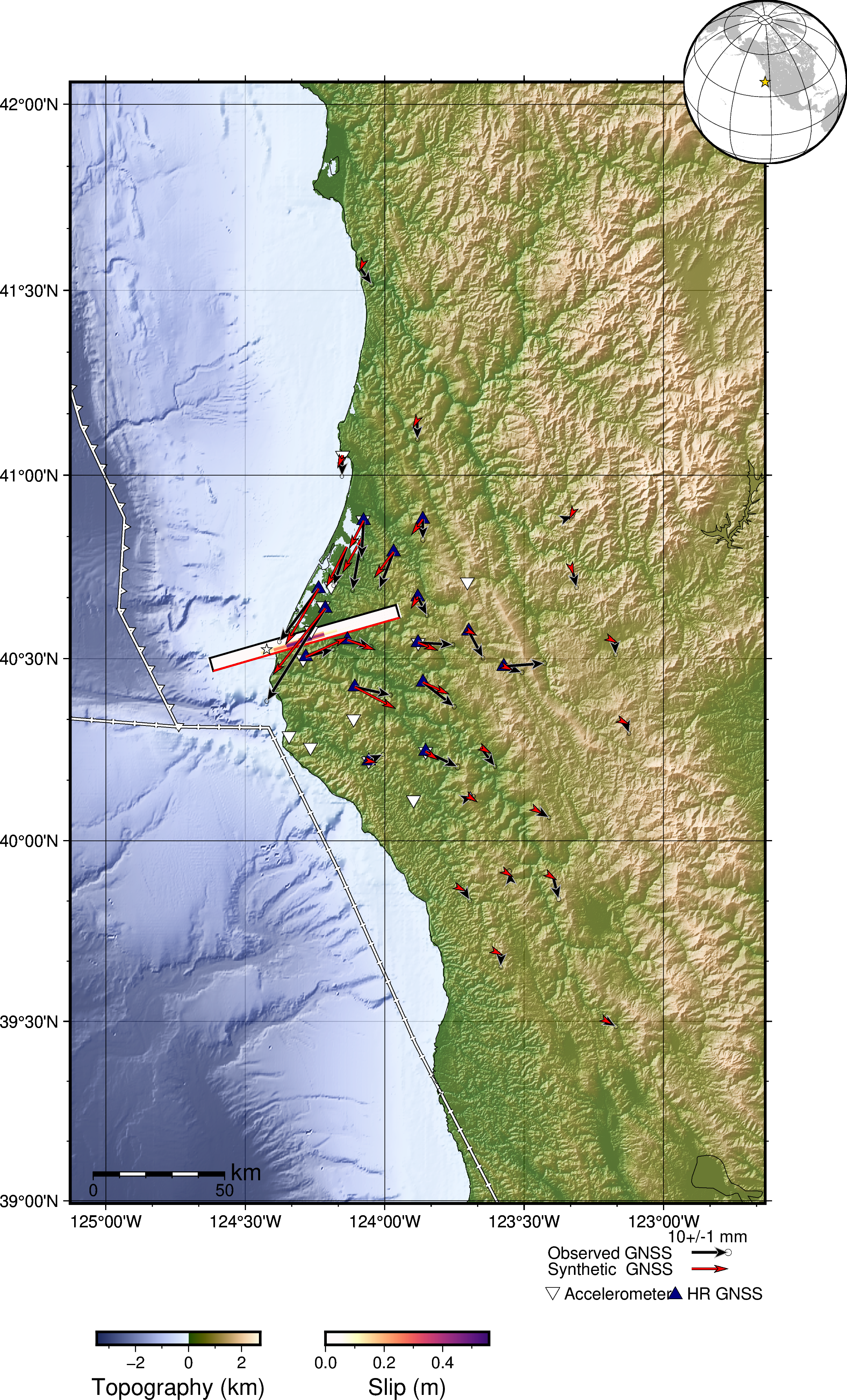
- Below is the USGS finite fault slip model and a comparison between the observed GNSS offsets and the offsets modeled by placing slip on the finite fault model in an elastic half space.
- Once we have better INSAR data (presuming these data will exist), this slip model may improve.
- Here is a map that shows the mapped geologic units. Some of the map is from McLaughlin et al. (2000) and some is from the California Division of Mines and Geology (CDMG, 1999) which is now the California Geological Survey.
- There are about 30 units in each dataset, so I chose to simply use their labels from the respective databases. The CDMG labels are basically the same as the geologic unit (e.g., Franciscan is something like TKJf) while McLaughlin mapped units relative to their geomorphic expression, so units have strange labels (e.g., Franciscan is something like co1 or cm1).
- Note that the seismicity trend from the M 6.4 does not align with the faults nor the geologic units in the North America plate. This makes the linkage between rupturing in the Gorda and the North America plates more tenuous (though still possible).
Aftershock Patterns
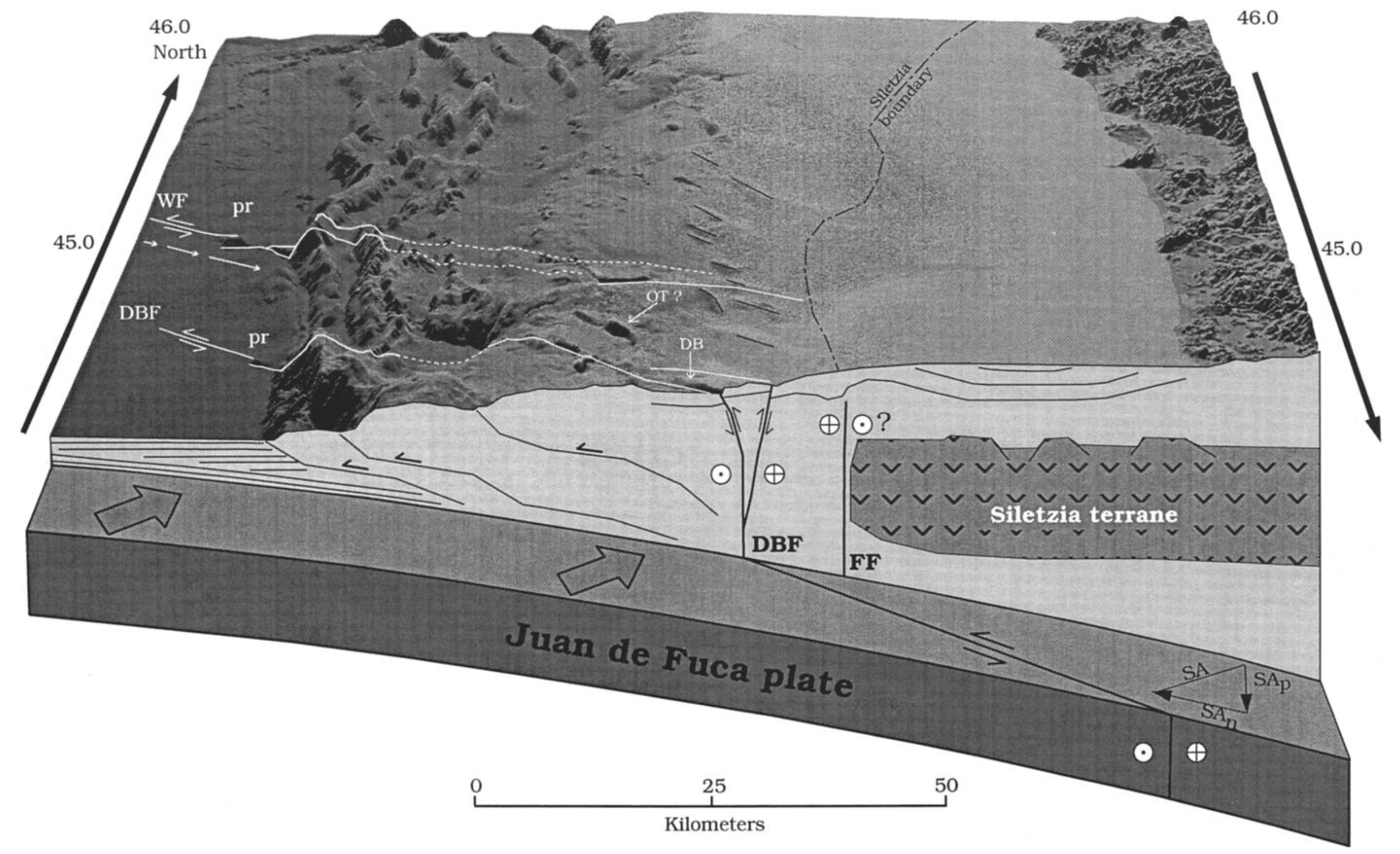
Block rotation model for the central Cascadia forearc. SeaBeam bathymetry shaded from the north. The Wecoma and Daisy Bank faults are show, with the Daisy Bank fault exposed in the foreground. Well-mapped fault traces are in solid; discontinuous traces are dashed. The arc-parallel component of oblique subduction creates a dextral share couple, which is accommodated by WNW trending left-lateral strike-slip faults. We propose that shearing of the slab due to oblique subduction is responsible for the fault involving oceanic crust. WF, Wecoma fault; DBF, Daisy bank fault; FF, Fulmar fault, “pr,” pressure ridge; “DB,” Daisy Bank; “OT?,” possible old left-lateral fault strand. Arrow heads and tails show strike-slip motion. White arrows at western end of Wecoma fault show eastward increasing slip calculated from isopach offsets.
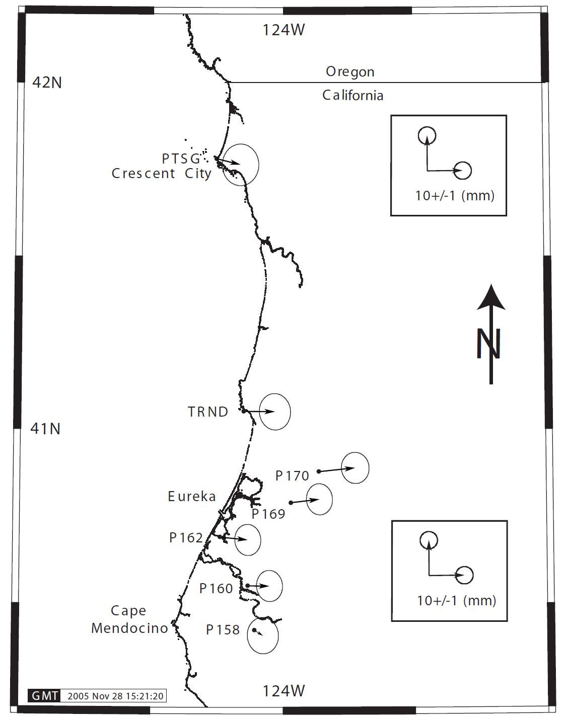
Coseismic displacements from the 15-Jun-2005 M7.2 Gorda plate earthquake located (off the map) 156 km (97 miles) W (280°) from Trinidad, CA and 157 km (98 miles) WSW (251°) from Crescent City, CA. Note the similarity to the deformation pattern of the 1994 event. Continuously operating GPS stations shown here are operated and maintained through the Plate Boundary Observatory component (pboweb.unavco. org) of the National Science Foundation’s EarthScope project
(www.earthscope.org).
Mapped Geology
- Here is the poster from last year’s earthquake sequence.
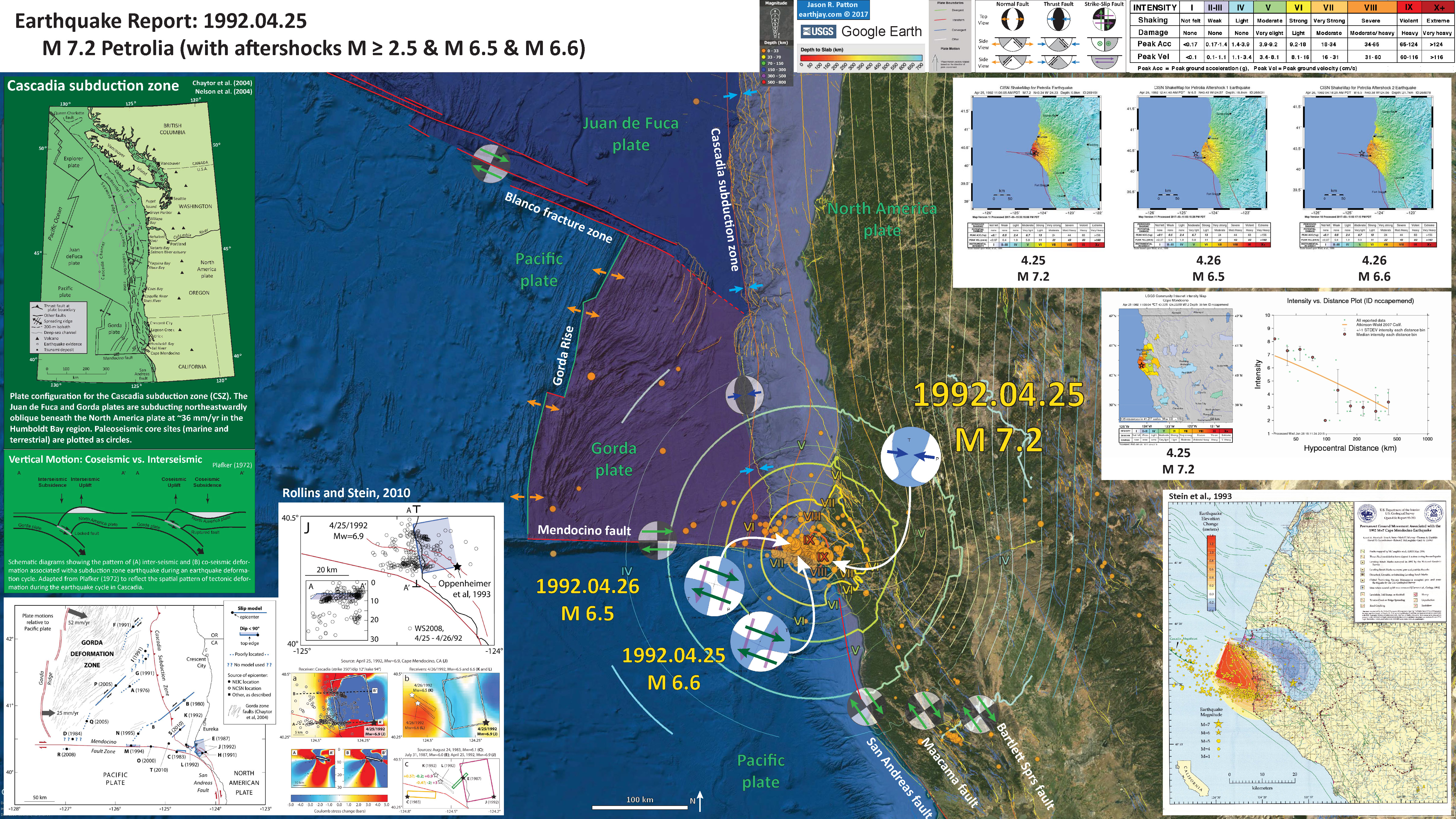
- Here are two relevant interpretive posters from the 1992 Cape Mendocino Earthquake.
- This one is an overview of the earthquake.
- This one helps us compare the mainshock and two main triggered earthquakes.
- Here is a poster that shows a comparison between the 1991 Honeydew and 1992 Cape Mendocino earthquakes..
Earlier Report Interpretive Posters


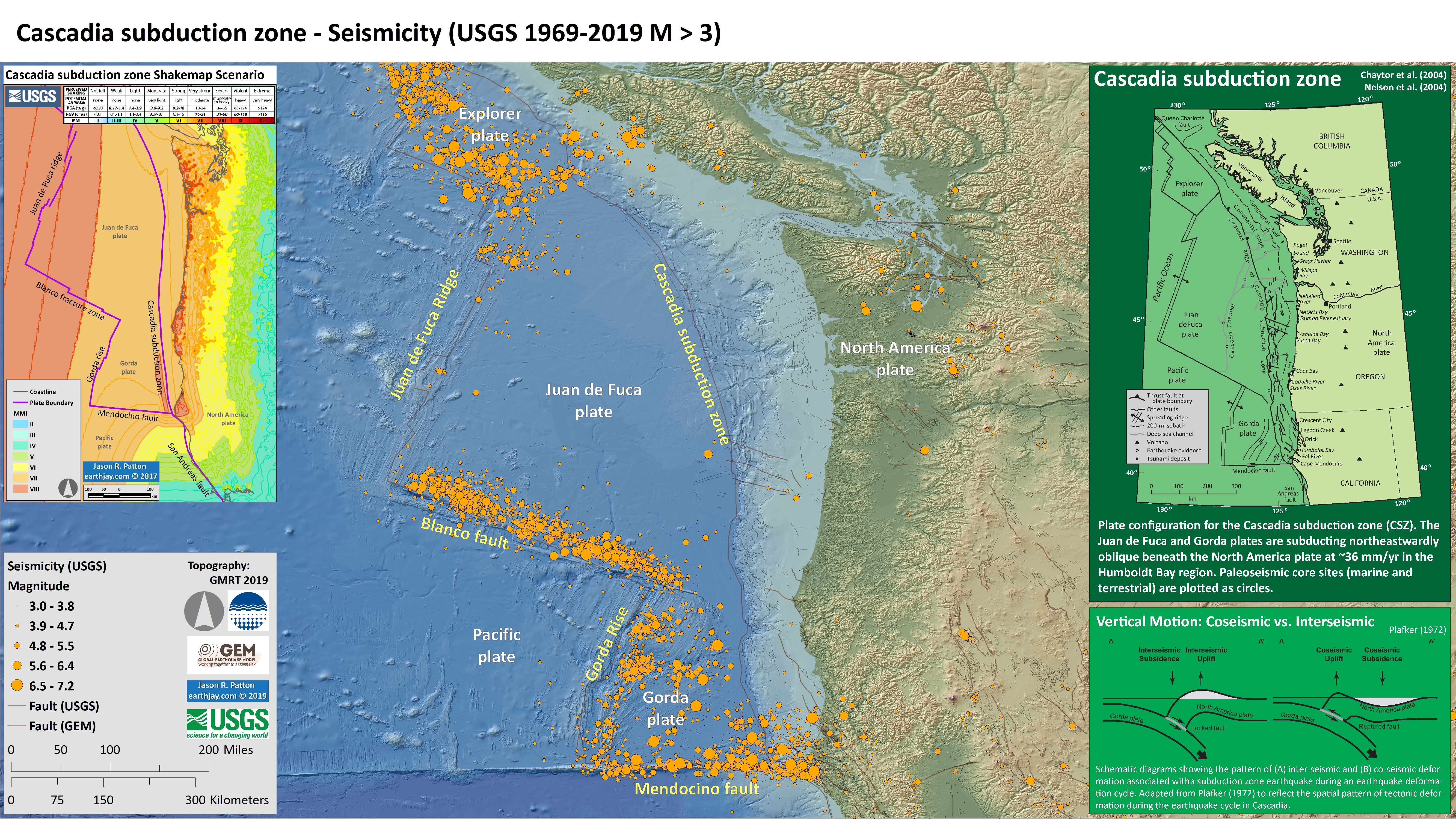
- Here is a map of the Cascadia subduction zone, modified from Nelson et al. (2006). The Juan de Fuca and Gorda plates subduct norteastwardly beneath the North America plate at rates ranging from 29- to 45-mm/yr. Sites where evidence of past earthquakes (paleoseismology) are denoted by white dots. Where there is also evidence for past CSZ tsunami, there are black dots. These paleoseismology sites are labeled (e.g. Humboldt Bay). Some submarine paleoseismology core sites are also shown as grey dots. The two main spreading ridges are not labeled, but the northern one is the Juan de Fuca ridge (where oceanic crust is formed for the Juan de Fuca plate) and the southern one is the Gorda rise (where the oceanic crust is formed for the Gorda plate).
- Here is a version of the CSZ cross section alone (Plafker, 1972). This shows two parts of the earthquake cycle: the interseismic part (between earthquakes) and the coseismic part (during earthquakes). Regions that experience uplift during the interseismic period tend to experience subsidence during the coseismic period.
- This poster includes seismicity from the past ~5 decades, for temblors M > 3.0. I also include the map and cross section as explained above. On the left is a map that shows the possible shaking intensity from a future CSZ earthquake.
- More about the materials on this poster can be found on this page.
- Hemphill-Haley, E., 1995. Diatom evidence for earthquake-induced subsidence and tsunami 300 yr ago in southern coastal Washington in GSA Bulletin, v. 107, p. 367-378.
- Nelson, A.R., Shennan, I., and Long, A.J., 1996. Identifying coseismic subsidence in tidal-wetland stratigraphic sequences at the Cascadia subduction zone of western North America in Journal of Geophysical Research, v. 101, p. 6115-6135.
- Atwater, B.F. and Hemphill-Haley, E., 1997. Recurrence Intervals for Great Earthquakes of the Past 3,500 Years at Northeastern Willapa Bay, Washington in U.S. Geological Survey Professional Paper 1576, Washington D.C., 119 pp.
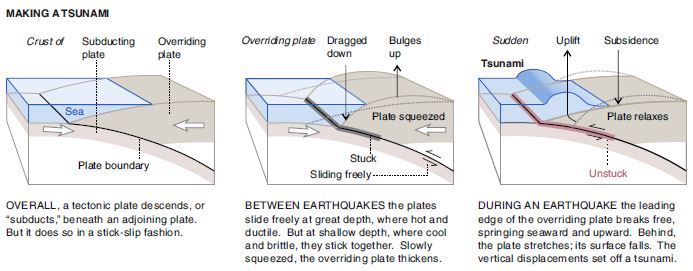
- This figure shows how a subduction zone deforms between (interseismic) and during (coseismic) earthquakes. We also can see how a subduction zone generates a tsunami. Atwater et al., 2005.
- Here is an animation produced by the folks at Cal Tech following the 2004 Sumatra-Andaman subduction zone earthquake. I have several posts about that earthquake here and here. One may learn more about this animation, as well as download this animation here.
- Here is a link to the embedded video below, showing the week-long seismicity in April 1992.
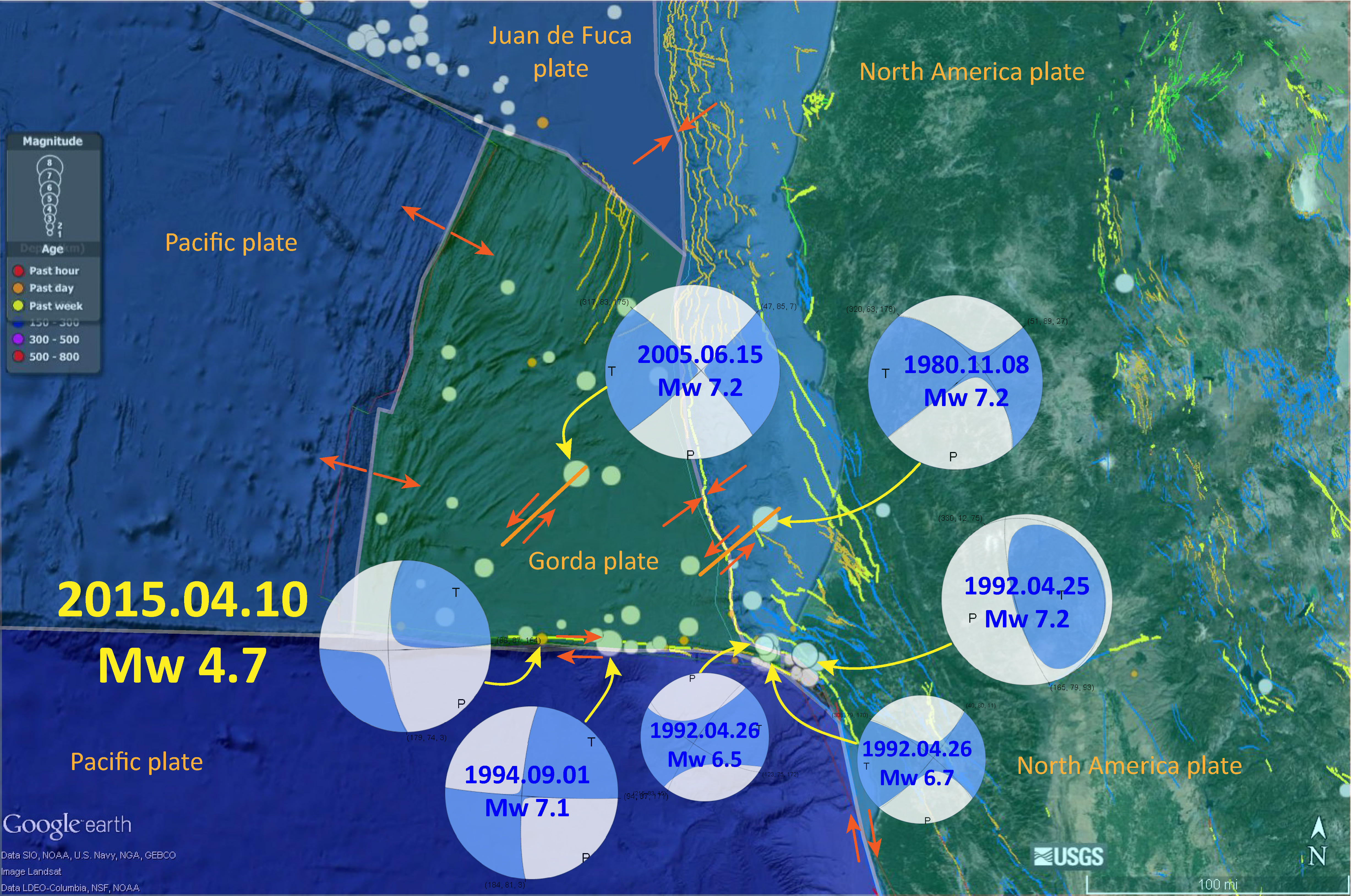
- This is the map used in the animation below. Earthquake epicenters are plotted (some with USGS moment tensors) for this region from 1917-2017 with M ≥ 6.5. I labeled the plates and shaded their general location in different colors.
- I include some inset maps.
- In the upper right corner is a map of the Cascadia subduction zone (Chaytor et al., 2004; Nelson et al., 2004).
- In the upper left corner is a map from Rollins and Stein (2010). They plot epicenters and fault lines involved in earthquakes between 1976 and 2010.
- Here is a map from Rollins and Stein, showing their interpretations of different historic earthquakes in the region. This was published in response to the Januray 2010 Gorda plate earthquake. The faults are from Chaytor et al. (2004).
- Here is a large scale map of the 1994 earthquake swarm. The mainshock epicenter is a black star and epicenters are denoted as white circles.
- Here is a plot of focal mechanisms from the Dengler et al. (1995) paper in California Geology.
Some Relevant Discussion and Figures
I have compiled some literature about the CSZ earthquake and tsunami. Here is a short list that might help us learn about what is contained within the core that I collected.
The Gorda and Juan de Fuca plates subduct beneath the North America plate to form the Cascadia subduction zone fault system. In 1992 there was a swarm of earthquakes with the magnitude Mw 7.2 Mainshock on 4/25. Initially this earthquake was interpreted to have been on the Cascadia subduction zone (CSZ). The moment tensor shows a compressional mechanism. However the two largest aftershocks on 4/26/1992 (Mw 6.5 and Mw 6.7), had strike-slip moment tensors. In my mind, these two aftershocks aligned on what may be the eastern extension of the Mendocino fault. However, looking at their locations, my mind was incorrect. These two earthquakes were not aftershocks, but were either left-lateral or right-lateral strike-slip Gorda plate earthquakes triggered by the M 7.1 thrust event.
These two quakes appear to be aligned with the two northwest trends in seismicity and the 18 March 2020 M 5.2. The orientation of the mechanisms are not as perfectly well aligned, but there are lots of reasons for this (perhaps the faults were formed in a slightly different orientation, but have rotated slightly).
There have been several series of intra-plate earthquakes in the Gorda plate. Two main shocks that I plot of this type of earthquake are the 1980 (Mw 7.2) and 2005 (Mw 7.2) earthquakes. I place orange lines approximately where the faults are that ruptured in 1980 and 2005. These are also plotted in the Rollins and Stein (2010) figure above. The Gorda plate is being deformed due to compression between the Pacific plate to the south and the Juan de Fuca plate to the north. Due to this north-south compression, the plate is deforming internally so that normal faults that formed at the spreading center (the Gorda Rise) are reactivated as left-lateral strike-slip faults. In 2014, there was another swarm of left-lateral earthquakes in the Gorda plate. I posted some material about the Gorda plate setting on this page.

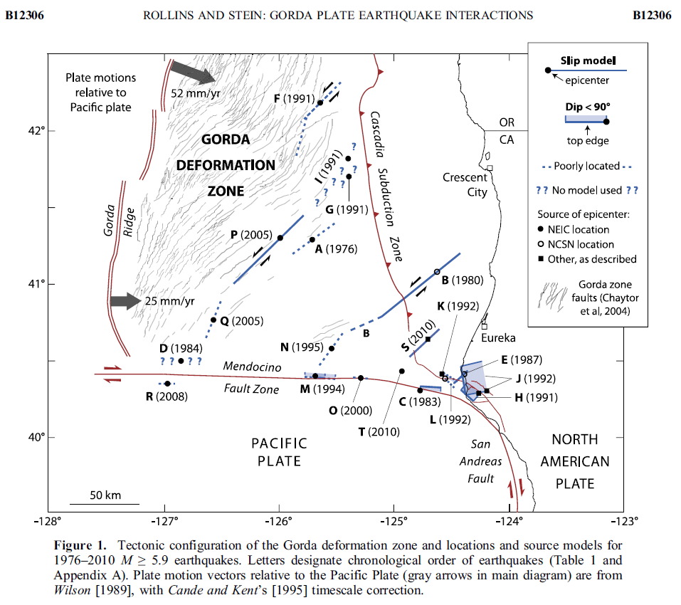
Tectonic configuration of the Gorda deformation zone and locations and source models for 1976–2010 M ≥ 5.9 earthquakes. Letters designate chronological order of earthquakes (Table 1 and Appendix A). Plate motion vectors relative to the Pacific Plate (gray arrows in main diagram) are from Wilson [1989], with Cande and Kent’s [1995] timescale correction.


- In this map below, I label a number of other significant earthquakes in this Mendocino triple junction region. Another historic right-lateral earthquake on the Mendocino fault system was in 1994. There was a series of earthquakes possibly along the easternmost section of the Mendocino fault system in late January 2015, here is my post about that earthquake series.
- Here is a map from Chaytor et al. (2004) that shows some details of the faulting in the region. The moment tensor (at the moment i write this) shows a north-south striking fault with a reverse or thrust faulting mechanism. While this region of faulting is dominated by strike slip faults (and most all prior earthquake moment tensors showed strike slip earthquakes), when strike slip faults bend, they can create compression (transpression) and extension (transtension). This transpressive or transtentional deformation may produce thrust/reverse earthquakes or normal fault earthquakes, respectively. The transverse ranges north of Los Angeles are an example of uplift/transpression due to the bend in the San Andreas fault in that region.
A: Mapped faults and fault-related ridges within Gorda plate based on basement structure and surface morphology, overlain on bathymetric contours (gray lines—250 m interval). Approximate boundaries of three structural segments are also shown. Black arrows indicated approximate location of possible northwest- trending large-scale folds. B, C: uninterpreted and interpreted enlargements of center of plate showing location of interpreted second-generation strike-slip faults and features that they appear to offset. OSC—overlapping spreading center.
- These are the models for tectonic deformation within the Gorda plate as presented by Jason Chaytor in 2004.
Models of brittle deformation for Gorda plate overlain on magnetic anomalies modified from Raff and Mason (1961). Models A–F were proposed prior to collection and analysis of full-plate multibeam data. Deformation model of Gulick et al. (2001) is included in model A. Model G represents modification of Stoddard’s (1987) flexural-slip model proposed in this paper.
Mendocino triple junction video
Shaking Intensity
- Here is a figure that shows a more detailed comparison between the modeled intensity and the reported intensity. Both data use the same color scale, the Modified Mercalli Intensity Scale (MMI). More about this can be found here. The colors and contours on the map are results from the USGS modeled intensity. The DYFI data are plotted as colored dots (color = MMI, diameter = number of reports).
- In the upper panel is the USGS Did You Feel It reports map, showing reports as colored dots using the MMI color scale. Underlain on this map are colored areas showing the USGS modeled estimate for shaking intensity (MMI scale).
- I also plot, in colored squares, the ground motions recorded on seismometers operated by the CGS Strong Motion Instrument Program (SMIP), run by Hamid Haddadi. Units are relative to gravitation acceleration where 1 = 1g. g is defined as the acceleration at the Earth’s surface (9.8 m/s^2). Here is the data page for this M 6.4 earthquake. The largest acceleration (1.36g) is from a seismometer attached to a bridge and seismologists think that this large acceleration is due to the bridge in some way. Here is the SMIP data page for the M 5.4 earthquake.
- Below the upper map plot is the USGS MMI Intensity scale, which lists the level of damage for each level of intensity, along with approximate measures of how strongly the ground shakes at these intensities, showing levels in acceleration (Peak Ground Acceleration, PGA) and velocity (Peak Ground Velocity, PGV).
- In the lower panel is a plot showing MMI intensity (vertical axis) relative to distance from the earthquake (horizontal axis). The models are represented by the green and orange lines. The DYFI data are plotted as light blue dots. The mean and median (different types of “average”) are plotted as orange and purple dots. Note how well (or poorly) the reports fit the brown line (the model that represents how MMI works based on quakes in California). The increased intensity on the left of the plot (which are closer to the earthquake) are the records that show intensities higher than expected from the modeling.
- Here is an animation from the USGS and Cal Tech that shows a simulation of seismic waves from this M 6.4 earthquake.
- There is a link to this video from the earthquake page.
Shaking Intensity and Potential for Ground Failure
- Below are a series of maps that show the shaking intensity and potential for landslides and liquefaction. These are all USGS data products.
- Below is the liquefaction susceptibility and landslide probability map (Jessee et al., 2017; Zhu et al., 2017). Please head over to that report for more information about the USGS Ground Failure products (landslides and liquefaction). Basically, earthquakes shake the ground and this ground shaking can cause landslides. We can see that there is a low probability for landslides. However, we have already seen photographic evidence for landslides and the lower limit for earthquake triggered landslides is magnitude M 5.5 (from Keefer 1984)
- I use the same color scheme that the USGS uses on their website. Note how the areas that are more likely to have experienced earthquake induced liquefaction are in the valleys. Learn more about how the USGS prepares these model results here.
There are many different ways in which a landslide can be triggered. The first order relations behind slope failure (landslides) is that the “resisting” forces that are preventing slope failure (e.g. the strength of the bedrock or soil) are overcome by the “driving” forces that are pushing this land downwards (e.g. gravity). The ratio of resisting forces to driving forces is called the Factor of Safety (FOS). We can write this ratio like this:
FOS = Resisting Force / Driving Force
When FOS > 1, the slope is stable and when FOS < 1, the slope fails and we get a landslide. The illustration below shows these relations. Note how the slope angle α can take part in this ratio (the steeper the slope, the greater impact of the mass of the slope can contribute to driving forces). The real world is more complicated than the simplified illustration below.

Landslide ground shaking can change the Factor of Safety in several ways that might increase the driving force or decrease the resisting force. Keefer (1984) studied a global data set of earthquake triggered landslides and found that larger earthquakes trigger larger and more numerous landslides across a larger area than do smaller earthquakes. Earthquakes can cause landslides because the seismic waves can cause the driving force to increase (the earthquake motions can “push” the land downwards), leading to a landslide. In addition, ground shaking can change the strength of these earth materials (a form of resisting force) with a process called liquefaction.
Sediment or soil strength is based upon the ability for sediment particles to push against each other without moving. This is a combination of friction and the forces exerted between these particles. This is loosely what we call the “angle of internal friction.” Liquefaction is a process by which pore pressure increases cause water to push out against the sediment particles so that they are no longer touching.
An analogy that some may be familiar with relates to a visit to the beach. When one is walking on the wet sand near the shoreline, the sand may hold the weight of our body generally pretty well. However, if we stop and vibrate our feet back and forth, this causes pore pressure to increase and we sink into the sand as the sand liquefies. Or, at least our feet sink into the sand.
Below is a diagram showing how an increase in pore pressure can push against the sediment particles so that they are not touching any more. This allows the particles to move around and this is why our feet sink in the sand in the analogy above. This is also what changes the strength of earth materials such that a landslide can be triggered.

Below is a diagram based upon a publication designed to educate the public about landslides and the processes that trigger them (USGS, 2004). Additional background information about landslide types can be found in Highland et al. (2008). There was a variety of landslide types that can be observed surrounding the earthquake region. So, this illustration can help people when they observing the landscape response to the earthquake whether they are using aerial imagery, photos in newspaper or website articles, or videos on social media. Will you be able to locate a landslide scarp or the toe of a landslide? This figure shows a rotational landslide, one where the land rotates along a curvilinear failure surface.

Seismic Hazard and Seismic Risk
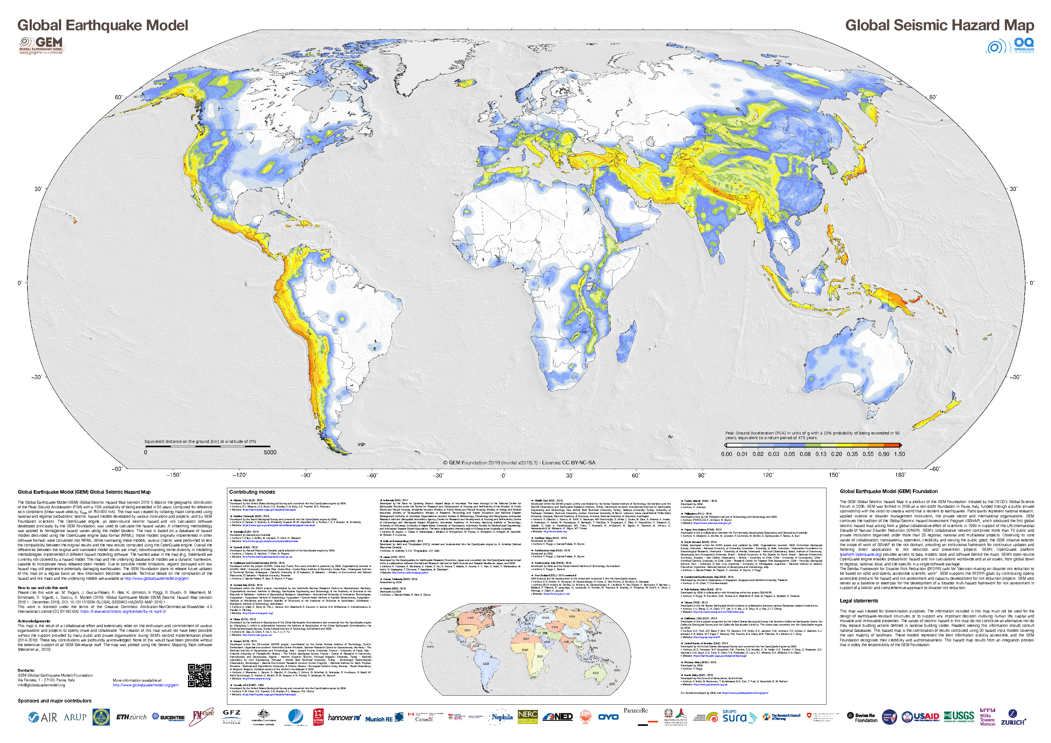
- These are two maps from the Global Earthquake Model (GEM) project, the GEM Seismic Hazard and the GEM Seismic Risk maps from Pagani et al. (2018) and Silva et al. (2018).
- The GEM Seismic Hazard Map:
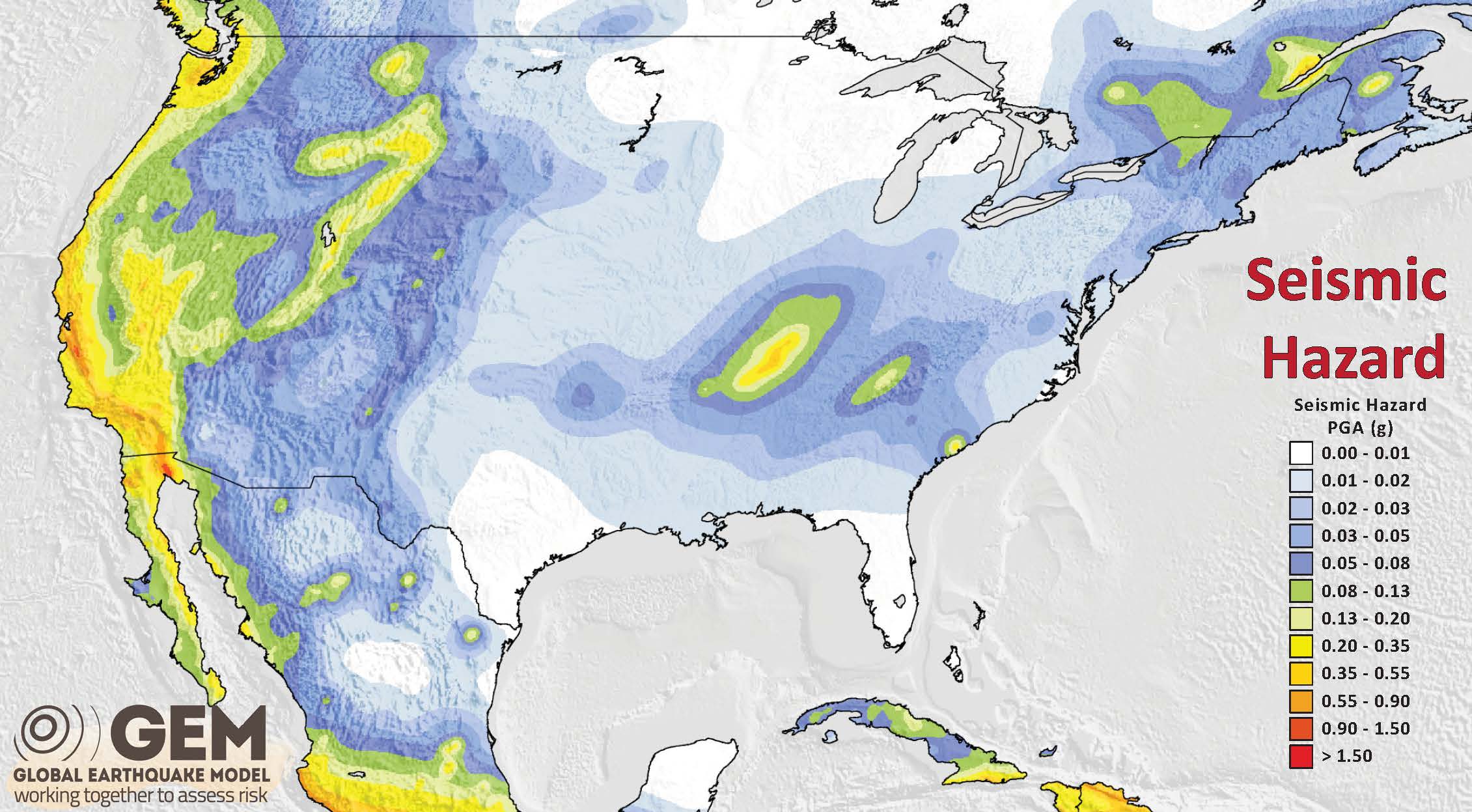
- The Global Earthquake Model (GEM) Global Seismic Hazard Map (version 2018.1) depicts the geographic distribution of the Peak Ground Acceleration (PGA) with a 10% probability of being exceeded in 50 years, computed for reference rock conditions (shear wave velocity, VS30, of 760-800 m/s). The map was created by collating maps computed using national and regional probabilistic seismic hazard models developed by various institutions and projects, and by GEM Foundation scientists. The OpenQuake engine, an open-source seismic hazard and risk calculation software developed principally by the GEM Foundation, was used to calculate the hazard values. A smoothing methodology was applied to homogenise hazard values along the model borders. The map is based on a database of hazard models described using the OpenQuake engine data format (NRML). Due to possible model limitations, regions portrayed with low hazard may still experience potentially damaging earthquakes.
- Here is a view of the GEM seismic hazard map for the USA.

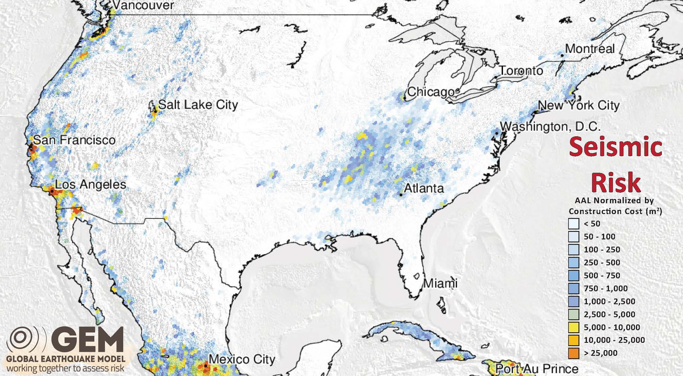
- The GEM Seismic Risk Map:
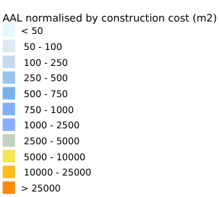
- The Global Seismic Risk Map (v2018.1) presents the geographic distribution of average annual loss (USD) normalised by the average construction costs of the respective country (USD/m2) due to ground shaking in the residential, commercial and industrial building stock, considering contents, structural and non-structural components. The normalised metric allows a direct comparison of the risk between countries with widely different construction costs. It does not consider the effects of tsunamis, liquefaction, landslides, and fires following earthquakes. The loss estimates are from direct physical damage to buildings due to shaking, and thus damage to infrastructure or indirect losses due to business interruption are not included. The average annual losses are presented on a hexagonal grid, with a spacing of 0.30 x 0.34 decimal degrees (approximately 1,000 km2 at the equator). The average annual losses were computed using the event-based calculator of the OpenQuake engine, an open-source software for seismic hazard and risk analysis developed by the GEM Foundation. The seismic hazard, exposure and vulnerability models employed in these calculations were provided by national institutions, or developed within the scope of regional programs or bilateral collaborations.
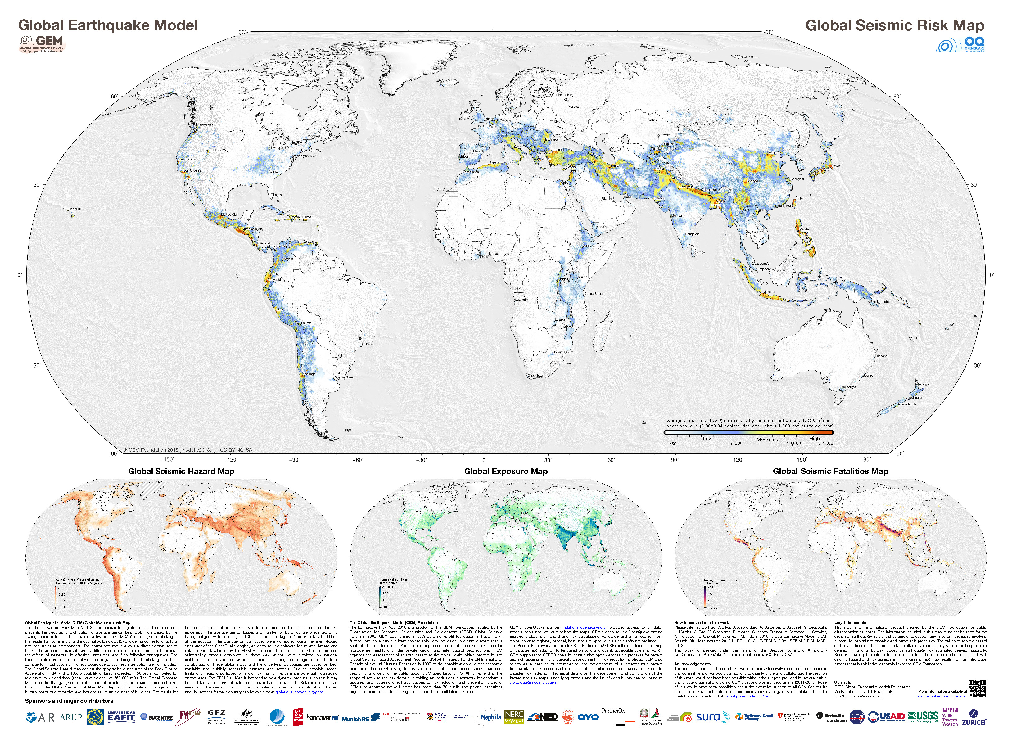
- Here is a view of the GEM seismic risk map for the USA. Note how the seismic risk is higher in places of larger population (like Los Angeles and San Francisco).
Stress Triggering
- When an earthquake fault slips, the crust surrounding the fault squishes and expands, deforming elastically (like in one’s underwear). These changes in shape of the crust cause earthquake fault stresses to change. These changes in stress can either increase or decrease the chance of another earthquake.
- I wrote more about this type of earthquake triggering for Temblor here. Head over there to learn more about “static coulomb stress triggering.”
- Rollins and Stein (2010) conducted this type of analysis for the 2010 M 6.5 Gorda Earthquake. They found that some of the faults in the region experienced an increase in fault stress (the red areas on the figure below). These changes in stress are very small, so require a fault to be at the “tipping point” for these changes in stress to cause an earthquake.
- There was a triggered earthquake in this sequence. There was a M 5.9 event about 25 days after the mainshock, this earthquake happened in a region that saw increased stress after the M 6.5. The M 5.9 appears to have been on the same fault as the M 6.5
- First, here is the fault model that Rollins and Stein used in their analysis of stress changes from the 2010 earthquake.
- Let’s take a look at some examples of analogic earthquakes to the 2010 temblor. First, here is a plot showing changes in stress following the 1980 Trinidad Earthquake (a very damaging earthquake in the region). This is the largest historic earthquake in the region at magnitude M 7.3 (other than the 1906 San Francisco Earthquake).
- Next let’s look at the stress changes following the 2005 M 7.2 earthquake.
- Here is the figure we have all been waiting for (actually, the next one is cool too). This figure shows the changes in stress associated with the 2010 M 6.5 earthquake. Remember, these are just models.
- This is the main take-away figure from Rollins and Stein (2010). For each map, there is a source fault (in black) and receiver faults (red or blue, depending on the change in stress).
- For example, in a, the source is a gorda plate left-lateral strike-slip fault. Parts of the Cascadia megathrust are represented on the right (triangles, labeled thrust). They also model changes in stress on the Mendocino fault (the red and blue lines at the bottom of “a”).
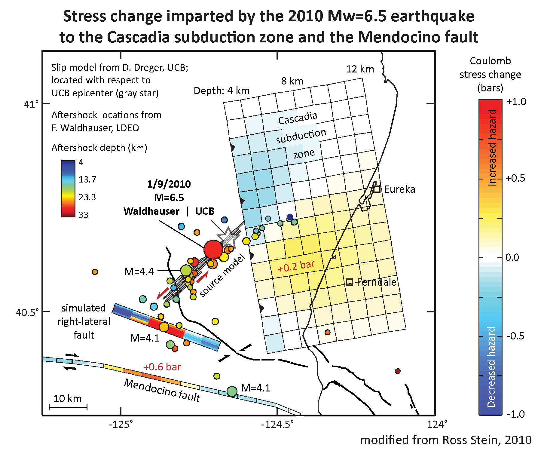
- And, you thought it couldn’t get any better. Here is yet another fantastic figure showing the stress change on the Cascadia megathrust fault and on the Mendocino fault following the 2010 M 6.5 earthquake.

Source models for earthquakes S and T, 10 January 2010, M = 6.5, and 4 February 2010, Mw = 5.9.

Coulomb stress changes imparted by the 1980 Mw = 7.3 earthquake (B) to a matrix of faults representing the Mendocino Fault Zone, the Cascadia subduction zone, and NE striking left‐lateral faults in the Gorda zone. The Mendocino Fault Zone is represented by right‐lateral faults whose strike rotates from 285° in the east to 270° in the west; Cascadia is represented by reverse faults striking 350° and dipping 9°; faults in the Gorda zone are represented by vertical left‐lateral faults striking 45°. The boundary between the left‐lateral “zone” and the reverse “zone” in the fault matrix is placed at the 6 km depth contour on Cascadia, approximated by extending the top edge of the Oppenheimer et al.
[1993] model for the 1992 Cape Mendocino earthquake (J). Calculation depth is 5 km. The numbered brackets are groups of aftershocks from Hill et al. [1990].

Coulomb stress changes imparted by the Shao and Ji (2005) variable slip model for the 15 June 2005 Mw = 7.2 earthquake (P) to the epicenter of the 17 June 2005 Mw = 6.6 earthquake (Q). Calculation depth is 10 km.

Coulomb stress changes imparted by the D. Dreger (unpublished report, 2010, [no longer] available at http://seismo.berkeley.edu/∼dreger/jan10210_ff_summary.pdf) model for the January 2010 M = 6.5 shock (S) to nearby faults. East of the dashed line, stress changes are resolved on the Cascadia subduction zone, represented by a northward extension of the Oppenheimer et al. [1993] rupture plane for the 1992 Mw = 6.9 Cape Mendocino earthquake. West of the dashed line, stress changes are resolved on the NW striking nodal plane for the February 2010 Mw = 5.9 earthquake (T) at a depth of 23.6 km.

- Here is a video that Ross Stein prepared as part of their analyses for this earthquake sequence. They include this in their Temblor report on this sequence here.
- 1700.09.26 M 9.0 Cascadia’s 315th Anniversary 2015.01.26
- 1700.09.26 M 9.0 Cascadia’s 316th Anniversary 2016.01.26 updated in 2017 and 2018
- 1992.04.25 M 7.1 Cape Mendocino 25 year remembrance
- 1992.04.25 M 7.1 Cape Mendocino 25 Year Remembrance Event Page
- Earthquake Information about the CSZ 2015.10.08
- 2022.12.20 M 6.4 Gorda plate
- 2021.12.20 M 5.7 & 6.2 Mendocino fault/Gorda plate
- 2020.05.18 M 5.5 Gorda Rise
- 2018.07.24 M 5.6 Gorda plate
- 2018.03.22 M 4.6/4.7 Gorda plate
- 2017.07.28 M 5.1 Gorda plate
- 2016.09.25 M 5.0 Gorda plate
- 2016.09.25 M 5.0 Gorda plate
- 2016.01.30 M 5.0 Gorda plate
- 2015.12.29 M 4.9 Gorda plate
- 2015.11.18 M 3.2 Gorda plate
- 2014.03.13 M 5.2 Gorda Rise
- 2014.03.09 M 6.8 Gorda plate p-1
- 2014.03.23 M 6.8 Gorda plate p-2
- 2010.01.10 M 6.5 Gorda plate
- 2019.08.29 M 6.3 Blanco transform fault
- 2018.08.22 M 6.2 Blanco transform fault
- 2018.07.29 M 5.3 Blanco transform fault
- 2015.06.01 M 5.8 Blanco transform fault p-1
- 2015.06.01 M 5.8 Blanco transform fault p-2 (animations)
- 2021.12.20 M 5.7 & 6.2 Mendocino fault
- 2020.03.09 M 5.8 Mendocino fault
- 2018.01.25 M 5.8 Mendocino fault
- 2017.09.22 M 5.7 Mendocino fault
- 2016.12.08 M 6.5 Mendocino fault, CA
- 2016.12.08 M 6.5 Mendocino fault, CA Update #1
- 2016.12.05 M 4.3 Petrolia CA
- 2016.10.27 M 4.1 Mendocino fault
- 2016.09.03 M 5.6 Mendocino
- 2016.01.02 M 4.5 Mendocino fault
- 2015.11.01 M 4.3 Mendocino fault
- 2015.01.28 M 5.7 Mendocino fault
- 2015.11.01 M 4.3 Mendocino fault
- 2015.01.28 M 5.7 Mendocino fault
- 2020.03.18 M 5.2 Petrolia
- 2019.06.23 M 5.6 Petrolia
- 2017.03.06 M 4.0 Cape Mendocino
- 2016.11.02 M 3.6 Oregon
- 2016.01.07 M 4.2 NAP(?)
- 2015.10.29 M 3.4 Bayside
- 2018.10.22 M 6.8 Explorer plate
- 2017.01.07 M 5.7 Explorer plate
- 2016.03.19 M 5.2 Explorer plate
- 2017.06.11 M 3.5 Gorda or NAP?
- 2016.07.21 M 4.7 Gorda or NAP? p-1
- 2016.07.21 M 4.7 Gorda or NAP? p-2
Cascadia subduction zone
General Overview
Earthquake Reports
Gorda plate
Blanco transform fault
Mendocino fault
Mendocino triple junction
North America plate
Explorer plate
Uncertain
Social Media
#EarthquakeReport for M 6.4 #Earthquake in Mendocino triple junction (Triangle of Doom) region
early to tell (if we learned from last year) left or right lateral strike-slip prob in Gorda plate
read more from last year's reporthttps://t.co/aS9ySr9YIPhttps://t.co/9HKHnpuwE9 pic.twitter.com/YZeimi6AC9
— Jason "Jay" R. Patton (@patton_cascadia) December 20, 2022
#EarthquakeReport for M 6.4 #Earthquake in Mendocino triple junction (Triangle of Doom) region
aftershocks suggest left-lateral strike-slip in Gorda plate
felt broadly, about 92%g in Ferndale
read more from last year's reporthttps://t.co/aS9ySrs7WXhttps://t.co/9HKHnpMFSh pic.twitter.com/wt4UduAuvt
— Jason "Jay" R. Patton (@patton_cascadia) December 20, 2022
#EarthquakeReport for M 6.4 #Earthquake offshore of #HumboldtCounty #California
intensity summary: @USGS_Quakes model vs Did You Feel It? observations
PGA in g units from https://t.co/KM7lTGSzX7
report forthcoming, 2021 review: https://t.co/aS9ySr9YIPhttps://t.co/9HKHnpuwE9 pic.twitter.com/K2JiOEKJTm
— Jason "Jay" R. Patton (@patton_cascadia) December 22, 2022
#EarthquakeReport for M 6.4 #Earthquake in #Humboldt County #California
interpretive poster showing aftershocks and comparison with '22 sequence
no foreshocks@USGS_Quakes slip/GNSS model compared with GNSS observations
report forthcoming, '22 report: https://t.co/aS9ySr9YIP pic.twitter.com/NfYkUuW13J
— Jason "Jay" R. Patton (@patton_cascadia) December 22, 2022
#EarthquakeReport for M6.4 #Earthquake offshore northern #California#FerndaleEarthquake
hypocenters from @USGS_Quakes
i plotted USGS Slab2 depths https://t.co/HdW0ZOzted
i traced Gorda slab from Guo 2021 B-B' https://t.co/t8gXg1jaYYread report herehttps://t.co/0rRNL3TfNk pic.twitter.com/Mni4dbD8Oo
— Jason "Jay" R. Patton (@patton_cascadia) December 24, 2022
#EarthquakeReport for M6.4 #Earthquake in #HumboldtCounty #California
Gorda intraplate left-lateral strike-slip earthquake
see: https://t.co/t8gXg1jaYYsome tensional mechanisms
possibly 2 main faults involved (?) outlined in white
read report herehttps://t.co/0rRNL3TfNk pic.twitter.com/FQripjzAa0
— Jason "Jay" R. Patton (@patton_cascadia) December 26, 2022
#EarthquakeReport for M 6.4 #Earthquake in northern @California
updated plot: hypocenters compared to Gorda crust and the @USGS_Quakes Finite Fault Model showing that most of the slip occurred in the NAP (not sure this is correct)
read more herehttps://t.co/0rRNL3TfNk pic.twitter.com/Nca4IimQ3z
— Jason "Jay" R. Patton (@patton_cascadia) December 26, 2022
#EarthquakeReport for M6.4 #Earthquake in northern #California
geology from CDMG '99 and McLaughlin et al. '00. units are labeled, so no legend (abt 30 units in each data set)
lack of upper plate structures oriented with 6.4 seismicity
read report here:https://t.co/0rRNL3TfNk pic.twitter.com/iyCQBCsxf4
— Jason "Jay" R. Patton (@patton_cascadia) December 26, 2022
a triple junction is defined as where three plate boundaries meet, not where three plates meet (though that is also true). the types of triple junctions (e.g., RRR, TTT, RFF) refer to the types of faults that meet there. https://t.co/zfP2DidN6Ihttps://t.co/CLUfzwNanj pic.twitter.com/t9O5RFstfY
— Jason "Jay" R. Patton (@patton_cascadia) December 30, 2022
#EarthquakeReport for M6.4 & 5.4 #Earthquakes in the #Triangleofdoom #Mendocinotriplejunction
M6.4 – left-lateral strike-slip (in crust?)
M5.4 – right-lateral s-s (in mantle?)updated aftershock map and hypocenter profile
read the report herehttps://t.co/0rRNL3TfNk pic.twitter.com/HNpiZRBP8a
— Jason "Jay" R. Patton (@patton_cascadia) January 3, 2023
The #earthquake stopped campus clocks at 2:34 AM. pic.twitter.com/PeQNwvL4I0
— Cal Poly Humboldt (@humboldtcalpoly) December 22, 2022
Good morning Redwood Coast CA. Did you feel the magnitude 6.4 quake about 7.5 miles southwest of Ferndale at 2:34 am? The #ShakeAlert system was activated. See: https://t.co/zwOapjTWaA pic.twitter.com/eMSUAT3inw
— USGS ShakeAlert (@USGS_ShakeAlert) December 20, 2022
A M6.4 earthquake has occurred south of Eureka, CA in northern CA (Humboldt Co.). Additional shaking from aftershocks is expected in the region. We are continuing to monitor this event, so check back for additional information. #Humboldt #earthquake pic.twitter.com/DpaIlz3RGV
— California Geological Survey (@CAGeoSurvey) December 20, 2022
A M6.4 earthquake & several aftershocks hit the coast near Ferndale, CA. Epicenter is close enough to land that strong shaking & some ground/structure damage is expected. #earthquake #Humboldt pic.twitter.com/YcO3mVEJCI
— Brian Olson (@mrbrianolson) December 20, 2022
#EarthquakeReport for M 6.4 #Earthquake in Mendocino triple junction (Triangle of Doom) region
felt broadly at least intensity MMI 8
read more from last year's reporthttps://t.co/aS9ySr9YIPhttps://t.co/9HKHnpuwE9 pic.twitter.com/8qAaSK6i9y
— Jason "Jay" R. Patton (@patton_cascadia) December 20, 2022
#EarthquakeReport for M 6.4 #Earthquake in Mendocino triple junction (Triangle of Doom) region
modest chance for eq triggred landslides
high likelihood for eq induced liquefactionread more from last year's reporthttps://t.co/aS9ySr9YIPhttps://t.co/RXs6q07wjX pic.twitter.com/zI9cPfnRUG
— Jason "Jay" R. Patton (@patton_cascadia) December 20, 2022
A few more clean signals pic.twitter.com/53tL2Rixkb
— Brendan Crowell (@bwcphd) December 20, 2022
That was a big one. Power is now out in #ferndaleca. House is a mess. #earthquake pic.twitter.com/YEmcv1Urhp
— Caroline Titus (@caroline95536) December 20, 2022
About 50,000 PG&E customers are without power in Humboldt after that earthquake, which was a preliminary magnitude 6.4.https://t.co/TLWiUpfEGp
— North Coast Journal (@ncj_of_humboldt) December 20, 2022
Road Closure: State Route 211 at Fernbridge, Humboldt County is CLOSED. The bridge is closed while we conduct safety inspections due to possible seismic damage. pic.twitter.com/601oOQRz2o
— Caltrans District 1 (@CaltransDist1) December 20, 2022
FERNBRIDGE EARTHQUAKE DAMAGE: Damage to Fernbridge following the 6.2 magnitude #earthquake in Humboldt County. Main road to Ferndale currently closed off by CalTrans as crews inspect for additional damage. pic.twitter.com/4BPOSvZrN9
— Austin Castro (@AustinCastroTV) December 20, 2022
Auto solution FMNEAR (Géoazur/OCA) with regional records for the M 6.3 – OFFSHORE NORTHERN CALIFORNIA – 2022-12-20 10:34:25 UTC (Loc EMSC used to trigger inversion).https://t.co/UHDsc1hVXA
Thanks to the seismic records provided in particular by IRIS, SCEDC pic.twitter.com/VOEflZWynp— Bertrand Delouis (@BertrandDelouis) December 20, 2022
Mw=6.4, NEAR COAST OF NORTHERN CALIF. (Depth: 9 km), 2022/12/20 10:34:25 UTC – Full details here: https://t.co/nC4QZqppm0 pic.twitter.com/QW0ggaT4dE
— Earthquakes (@geoscope_ipgp) December 20, 2022
strong #Earthquake offshore California, United States Of America
Felt by at least 9.0 m. people.
More than 130k people live in regions, where damage can be expected.
Severe damage is expected in an area affecting more than 50k people.https://t.co/9Ku6UPu3gQ pic.twitter.com/6UN4tIasme— CATnews (@CATnewsDE) December 20, 2022
The area where this quake occurred is quite active. These images from @EarthScope_sci IRIS Earthquake Browser show earthquakes in the area of M4+, M5+, M6+ and M7+. pic.twitter.com/y3xafBrCfd
— Wendy Bohon, PhD 🌏 (@DrWendyRocks) December 20, 2022
In fact, there have already been 20+ aftershocks of M2.5+! Again, this is normal and expected.
PSA: aftershocks are just smaller earthquakes that occur after a larger quake.
Here’s more info https://t.co/byWunrqSqZ
— Wendy Bohon, PhD 🌏 (@DrWendyRocks) December 20, 2022
— Robert Martin (@NordBob) December 20, 2022
Following the M6.4 mainshock, there have been well over 20 recorded aftershocks above M2.5. pic.twitter.com/Gej6rRNDlG
— EarthScope Consortium (@EarthScope_sci) December 20, 2022
Saw this on Facebook from someone in Eureka after tonight's quake. A reminder to "Secure Your Space" by tethering heavy furniture to the wall for this exact reason. #earthquake pic.twitter.com/1CiYbLOQcE
— Brian Olson (@mrbrianolson) December 20, 2022
Some people in Los Angeles and Tacoma really need to chill out and have less caffeine before bed 🧐🤔 https://t.co/5zIRhUR6eq pic.twitter.com/iURHlVVuOS
— Austin Elliott (@TTremblingEarth) December 20, 2022
Just took a cruise down Main Street #ferndaleca. Couldn’t see one broken window. Many store owners replaced broken ones after 6.2 on this same day in 2021. Also today’s #earthquake shook north/south. #earthquakeca pic.twitter.com/Ua1nMx0UuJ
— Caroline Titus (@caroline95536) December 20, 2022
Ferndale M6.4 strike-slip earthquake and aftershocks so far, all lining up along the left-lateral nodal plane of the focal mechanism. pic.twitter.com/lfWX5Qz4FF
— Harold Tobin (@Harold_Tobin) December 20, 2022
M6.4 #earthquake near Ferndale, CA: Seismicity for today (red), the past year (orange) and back to 1982 (green-blue-purple). Views from above/south/east. Today's events may be in upper part of down-going, Gorda plate. pic.twitter.com/WdvPq85LJP
— Anthony Lomax 😷🇪🇺🌍🇺🇦 (@ALomaxNet) December 20, 2022
Cal OES is coordinating with local and tribal governments to assess the impacts of the Earthquake and supporting with resources, mutual aid and damage assessment. State Agency response including Cal OES, Cal Fire, Cal Trans, Cal CGS, CHP in support of local efforts
— California Governor's Office of Emergency Services (@Cal_OES) December 20, 2022
Peak ground acceleration plot of seismic stations that recorded shaking from last night's M6.4 earthquake in Humboldt County. Notably, several values are *WELL* above the predicted envelope given distance from the epicenter. Is this real? Any explanations? Near-field effect? pic.twitter.com/QHdAMlglbM
— Brian Olson (@mrbrianolson) December 20, 2022
A brief explainer about the M6.4 earthquake near Ferndale in Northern California pic.twitter.com/3Ar03QFlC3
— Wendy Bohon, PhD 🌏 (@DrWendyRocks) December 20, 2022
Gov. Newsom & State officials provide updates on the M6.4 earthquake today near Ferndale in Humboldt County. #earthquake #Eureka @Cal_OES @GovPressOffice https://t.co/xHAkna9UYw
— California Geological Survey (@CAGeoSurvey) December 20, 2022
Cindy Pridmore representing CGS at today's press conference on the M6.4 Ferndale earthquake. She noted quakes of this size aren't uncommon here & people should be aware of continuing aftershocks, especially if they are in structures already damaged by the quake. @CAGeoSurvey pic.twitter.com/hRrJkLT7Tz
— Brian Olson (@mrbrianolson) December 20, 2022
Small teams of CGS geologists are currently out in the Ferndale, Rio Dell, & Eureka areas documenting structural & ground damage from this morning's M6.4 earthquake. Seeing where damage occurs helps us understand how shaking intensity & damage are related. #earthquake #humboldt
— California Geological Survey (@CAGeoSurvey) December 20, 2022
The @USGS_Quakes aftershock forecast for the M6.4 event in Northern California is out.
MOST LIKELY – “There will likely be smaller aftershocks within the next week with up to 24 M3+ aftershocks. M3+ aftershocks are large enough to be felt nearby.” https://t.co/7o2iJhozp0
— Wendy Bohon, PhD 🌏 (@DrWendyRocks) December 20, 2022
Important info for folks that live in Earthquake country 👇🏻 https://t.co/ZGWNf1zYpr
— Wendy Bohon, PhD 🌏 (@DrWendyRocks) December 20, 2022
Sadly, two reported deaths.
https://t.co/s2By2z6zDh— Jason "Jay" R. Patton (@patton_cascadia) December 20, 2022
This Magnitude 6.4 earthquake in California and subsequent power outage got me wanting to share this new video guide on small scale solar back up now.
This is the short version of the video based on this step-by-step guide – https://t.co/af5okVx2P7#photovoltaics #prepper pic.twitter.com/oxmYbiNQ9i
— Lonny Grafman (@LonnyGrafman) December 20, 2022
Seismicity map of today's Ferndale earthquakes with red outline (suggesting EW plane may be fault), and the events from exactly a year ago in purple. A bit confusing, since the M6.2 from a year ago appears to have been relocated significantly from its original offshore location. pic.twitter.com/K3HvECUt4l
— Jascha Polet (@CPPGeophysics) December 20, 2022
Still not seeing many images of damage, but based on anecdotes from folks in quake zone it does sound like there was damage to some structures & especially to infrastructure. I suspect that ongoing widespread regional power outages are reason we haven't heard more yet.#earthquake https://t.co/ACvlDpvqJR pic.twitter.com/ejHBRaMOHJ
— Daniel Swain (@Weather_West) December 20, 2022
Before (May 2018) & After (today) photos of the old Humboldt Creamery building in Loleta (across from the Cheese Factory). Old brick buildings perform so badly during earthquakes. I hope the cheese factory is safe.🧀🥛 #FerndaleEarthquake #earthquake pic.twitter.com/aMbbpsrsz6
— Brian Olson (@mrbrianolson) December 20, 2022
Some excellent 5-Hz GNSS velocities for the Ferndale EQ showing some strong site amplification at @EarthScope_sci site P168 (peak 35 cm/s). Closest seismic site KNEE is in good agreement. pic.twitter.com/OSskpMEMjX
— Brendan Crowell (@bwcphd) December 21, 2022
Wow! Extreme ground accelerations, well above 1 g, during the recent M6.4 earthquake near Ferndale, Caifornia, recorded in Rio Dell: https://t.co/HmJa5feZ3g
(preliminary data processing) https://t.co/7RGCxkHmZ5 pic.twitter.com/4FiIYo5EDC— Pablo Ampuero (@DocTerremoto) December 20, 2022
Governor @GavinNewsom proclaimed a state of emergency for Humboldt County to support the emergency response to today’s 6.4 magnitude earthquake near the City of Ferndale. https://t.co/EieUtBovqT
— Office of the Governor of California (@CAgovernor) December 21, 2022
'Significant' Damages in Rio Dell Area, Says Humboldt Office of Emergency Services; 11 Injuries, Two Dead from Medical Emergencies https://t.co/ruNr3ma5tN
— Lost Coast Outpost (@LCOutpost) December 20, 2022
Road damage from Northern California earthquake, in Rio Dell pic.twitter.com/P9eSSX4kRU
— EthanBaron (@ethanbaron) December 21, 2022
Over 3 million people in California & Oregon received #ShakeAlert-powered alerts during today’s M6.4 quake near Ferndale, CA. #ShakeAlert is success because of: @Cal_OES @OregonOEM @waEMD @waDNR @CAGeoSurvey @OregonGeology @OHAZ_UO @UW @PNSN1 @CaltechSeismo @BerkeleySeismo @USGS pic.twitter.com/wWL4N6aMxI
— USGS ShakeAlert (@USGS_ShakeAlert) December 20, 2022
Watching observations from this morning’s #earthquake come in: Some from our @CAGeoSurvey geologists and others gleaned from news reports and social media by our GIS professionals. Most of these are damage reports so far. Incredibly valuable spatial data! pic.twitter.com/JUPIV2AAtR
— Tim Dawson (@timblor) December 20, 2022
Real-time GNSS displacements recorded by GSeisRT for the Ferndale M6.4 event on Dec. 20th. @EarthScope_sci pic.twitter.com/HZz6F758l5
— Jianghui Geng (@GengJianghui) December 21, 2022
Our field teams were out documenting structural & ground damage yesterday to help us understand the shaking effects from yesterday's M6.4 Ferndale earthquake.
Most vulnerable to any strong shaking are "unreinforced masonry" buildings like the old Humboldt Creamery in Loleta. 1/7 pic.twitter.com/ZCInnRJv6k— California Geological Survey (@CAGeoSurvey) December 21, 2022
Learn more about the M6.4 earthquake near Ferndale, CA in this @USGS featured story : https://t.co/T5EYMvlKK5 @USGS_Quakes @CAGeoSurvey @Cal_OES @OregonOEM @OHAZ_UO @PNSN1 @waDNR @waShakeOut @ShakeOut @ECA @CalConservation @CaltechSeismo @BerkeleySeismo @ListosCA @FEMARegion9 pic.twitter.com/mgPPGQeM54
— USGS ShakeAlert (@USGS_ShakeAlert) December 21, 2022
Regarding the North Coast earthquake, my undergrad Geography advisor, Eugenie Rovai (Rio Dell local), did social geography research after the 1994 earthquake, and wrote about how history affected the capacity for each community to recover. https://t.co/eY4LXrGekl pic.twitter.com/HuWTkzyjVJ
— Zeke Lunder ~ The Lookout (@wildland_zko) December 22, 2022
The earthquake waves from the M6.4 Ferndale quake were recorded by seismic stations across North America. By the time the waves move away from the region where the earthquake occurred they are much too small to feel but not too small to measure. pic.twitter.com/s7UYGUjPey
— Wendy Bohon, PhD 🌏 (@DrWendyRocks) December 22, 2022
The supercomputer has finished chugging. Here is a preliminary simulation of how yesterday’s M6.4 earthquake might have focused shaking in specific areas. Event page here: https://t.co/UA9LAh0bJ2 pic.twitter.com/bdR9ZFYapn
— USGS Earthquakes (@USGS_Quakes) December 21, 2022
What’s the difference between geologic hazard and risk? What are the USGS National Seismic Hazard Maps, and how are they used? Find out in this introduction to the National Seismic Hazard Maps: https://t.co/biDoY1ewWx#SeismicHazards #Earthquakes pic.twitter.com/T48ytJ7gKJ
— USGS (@USGS) December 22, 2022
CA worked night and day and — less than 48 hours after a strong earthquake in Humboldt County — power has been restored to all communities.
Thank you @Cal_OES, @CaltransHQ, @CAL_FIRE, @CA_EMSA, and @CHP_HQ for helping recovery efforts.https://t.co/JIaFUWJO9A
— Office of the Governor of California (@CAgovernor) December 23, 2022
And the corresponding map view.
High-precision relocations of M≥2 1982 to 2021/12 done with NLL-SSST-coherence (https://t.co/EwE8DRzwvU), past year done with NLL-SSST.
Earthquake arrival data from https://t.co/7TWxvNHnee pic.twitter.com/KVN606rFfC
— Anthony Lomax 😷🇪🇺🌍🇺🇦 (@ALomaxNet) December 22, 2022
The 12/20/22 M6.4 earthquake has produced a nice aftershock sequence that illuminates the fault that likely ruptured. A nice zone northeast of the epicenter. @CAGeoSurvey found no surface rupture, so this is a seismologist’s earthquake with lots to learn. pic.twitter.com/XJB8MuJPno
— Tim Dawson (@timblor) December 24, 2022
ARIA has processed interferograms with 23 December Copernicus Sentinel-1 covering M6.4 Ferndale earthquake. Geocoded UNWrapped (GUNW) interf. files available from NASA ASF archive. @iamgracebato did InSAR time-series with MintPy to mitigate atmosphere in attached map. pic.twitter.com/6zqOpGFzD0
— Advanced Rapid Imaging & Analysis (ARIA) (@aria_hazards) December 24, 2022
HUMBOLDT OES: Around 70 Local Buildings Deemed Unsafe in the Wake of the Quakes, in Total; Here is the Big List of Resources for People Who Need Help https://t.co/yTizDPCnE5
— Lost Coast Outpost (@LCOutpost) January 3, 2023
- Frisch, W., Meschede, M., Blakey, R., 2011. Plate Tectonics, Springer-Verlag, London, 213 pp.
- Hayes, G., 2018, Slab2 – A Comprehensive Subduction Zone Geometry Model: U.S. Geological Survey data release, https://doi.org/10.5066/F7PV6JNV.
- Holt, W. E., C. Kreemer, A. J. Haines, L. Estey, C. Meertens, G. Blewitt, and D. Lavallee (2005), Project helps constrain continental dynamics and seismic hazards, Eos Trans. AGU, 86(41), 383–387, , https://doi.org/10.1029/2005EO410002. /li>
- Jessee, M.A.N., Hamburger, M. W., Allstadt, K., Wald, D. J., Robeson, S. M., Tanyas, H., et al. (2018). A global empirical model for near-real-time assessment of seismically induced landslides. Journal of Geophysical Research: Earth Surface, 123, 1835–1859. https://doi.org/10.1029/2017JF004494
- Kreemer, C., J. Haines, W. Holt, G. Blewitt, and D. Lavallee (2000), On the determination of a global strain rate model, Geophys. J. Int., 52(10), 765–770.
- Kreemer, C., W. E. Holt, and A. J. Haines (2003), An integrated global model of present-day plate motions and plate boundary deformation, Geophys. J. Int., 154(1), 8–34, , https://doi.org/10.1046/j.1365-246X.2003.01917.x.
- Kreemer, C., G. Blewitt, E.C. Klein, 2014. A geodetic plate motion and Global Strain Rate Model in Geochemistry, Geophysics, Geosystems, v. 15, p. 3849-3889, https://doi.org/10.1002/2014GC005407.
- Meyer, B., Saltus, R., Chulliat, a., 2017. EMAG2: Earth Magnetic Anomaly Grid (2-arc-minute resolution) Version 3. National Centers for Environmental Information, NOAA. Model. https://doi.org/10.7289/V5H70CVX
- Müller, R.D., Sdrolias, M., Gaina, C. and Roest, W.R., 2008, Age spreading rates and spreading asymmetry of the world’s ocean crust in Geochemistry, Geophysics, Geosystems, 9, Q04006, https://doi.org/10.1029/2007GC001743
- Pagani, M., J. Garcia-Pelaez, R. Gee, K. Johnson, V. Poggi, R. Styron, G. Weatherill, M. Simionato, D. Viganò, L. Danciu, D. Monelli (2018). Global Earthquake Model (GEM) Seismic Hazard Map (version 2018.1 – December 2018), DOI: 10.13117/GEM-GLOBAL-SEISMIC-HAZARD-MAP-2018.1
- Silva, V ., D Amo-Oduro, A Calderon, J Dabbeek, V Despotaki, L Martins, A Rao, M Simionato, D Viganò, C Yepes, A Acevedo, N Horspool, H Crowley, K Jaiswal, M Journeay, M Pittore, 2018. Global Earthquake Model (GEM) Seismic Risk Map (version 2018.1). https://doi.org/10.13117/GEM-GLOBAL-SEISMIC-RISK-MAP-2018.1
- Zhu, J., Baise, L. G., Thompson, E. M., 2017, An Updated Geospatial Liquefaction Model for Global Application, Bulletin of the Seismological Society of America, 107, p 1365-1385, https://doi.org/0.1785/0120160198
- Atwater, B.F., Musumi-Rokkaku, S., Satake, K., Tsuju, Y., Eueda, K., and Yamaguchi, D.K., 2005. The Orphan Tsunami of 1700—Japanese Clues to a Parent Earthquake in North America, USGS Professional Paper 1707, USGS, Reston, VA, 144 pp.
- Chaytor, J.D., Goldfinger, C., Dziak, R.P., and Fox, C.G., 2004. Active deformation of the Gorda plate: Constraining deformation models with new geophysical data: Geology v. 32, p. 353-356.
- Dengler, L.A., Moley, K.M., McPherson, R.C., Pasyanos, M., Dewey, J.W., and Murray, M., 1995. The September 1, 1994 Mendocino Fault Earthquake, California Geology, Marc/April 1995, p. 43-53.
- Geist, E.L. and Andrews D.J., 2000. Slip rates on San Francisco Bay area faults from anelastic deformation of the continental lithosphere, Journal of Geophysical Research, v. 105, no. B11, p. 25,543-25,552.
- Guo, H., McGuire, J., and Zhang, H., 2021. Correlation of porosity variations and rheological transitions on the southern Cascadia megathrust in Nature Geoscience, https://doi.org/10.1038/s41561-021-00740-1
- Irwin, W.P., 1990. Quaternary deformation, in Wallace, R.E. (ed.), 1990, The San Andreas Fault system, California: U.S. Geological Survey Professional Paper 1515, online at: http://pubs.usgs.gov/pp/1990/1515/
- Wilson, D.S., 2002. The Juan de Fuca plate and slab: Isochron structure and Cenozoic plate motions in Kirby, S., Wang, K., and Dunlop, S., The Cascadia Subduction Zone and Related Subduction Systems: Seismic Structure, Intraslab Earthquakes and Processes, and Earthquake Hazards, U.S. Geological Survey Open-File Report 02-328, Geological Survey of Canada Open File 4350, 182 pp., https://pubs.usgs.gov/of/2002/0328/
- McCrory, P.A.,. Blair, J.L., Waldhauser, F., kand Oppenheimer, D.H., 2012. Juan de Fuca slab geometry and its relation to Wadati-Benioff zone seismicity in JGR, v. 117, B09306, doi:10.1029/2012JB009407.
- McLaughlin, R.J., Ellen, S.D., Blake, M.C. Jr., Jayko, A.S., Irwin, W.P., Aalto, F.R., Carver, G.A., and Clarke, S.H. Jr., 2000. Geology of the Cape Mendocino, Eureka, Garberville, and Southwestern Part of the Hayfork 30 x 60 Minute Quadrangles and Adjacent Offshore Area, Northern California, USGS Miscellaneous Field Studies Map MF-2336, http://pubs.usgs.gov/mf/2000/2336/
- McLaughlin, R.J., Sarna-Wojcicki, A.M., Wagner, D.L., Fleck, R.J., Langenheim, V.E., Jachens, R.C., Clahan, K., and Allen, J.R., 2012. Evolution of the Rodgers Creek–Maacama right-lateral fault system and associated basins east of the northward-migrating Mendocino Triple Junction, northern California in Geosphere, v. 8, no. 2., p. 342-373.
- Nelson, A.R., Asquith, A.C., and Grant, W.C., 2004. Great Earthquakes and Tsunamis of the Past 2000 Years at the Salmon River Estuary, Central Oregon Coast, USA: Bulletin of the Seismological Society of America, Vol. 94, No. 4, pp. 1276–1292
- Rollins, J.C. and Stein, R.S., 2010. Coulomb stress interactions among M ≥ 5.9 earthquakes in the Gorda deformation zone and on the Mendocino Fault Zone, Cascadia subduction zone, and northern San Andreas Fault: Journal of Geophysical Research, v. 115, B12306, doi:10.1029/2009JB007117, 2010.
- Stoffer, P.W., 2006, Where’s the San Andreas Fault? A guidebook to tracing the fault on public lands in the San Francisco Bay region: U.S. Geological Survey General Interest Publication 16, 123 p., online at http://pubs.usgs.gov/gip/2006/16/
- Wallace, Robert E., ed., 1990, The San Andreas fault system, California: U.S. Geological Survey Professional Paper 1515, 283 p. [http://pubs.usgs.gov/pp/1988/1434/].
- Wells, D.L., and Coopersmith, K.J., 1994. New empirical relationships among magnitude, rupture length, rupture width, rupture area, and surface displacement in BSSA, v. 84, no. 4, p. 974-1002
- Wells, R.E., Blakely, R.J., Wech, A.G., McCrory, P.A., Michael, A., 2017. Cascadia subduction tremor muted by crustal faults in Geology, v. 45, no. 6, p. 515–518, https://doi.org/10.1130/G38835.1
- Williams, T.B. and McPherson, R.C., (2006). Gorda Plate Deformation Contributes to Shortening Between the Klamath Block and the On-land Portion of the Accretionary Prism to the S. Cascadia Subduction Zone. In Hemphill-Haley, M., McPherson, R., Patton, J. R., Stallman, J., Leroy, T.H., Sutherland, D., and Williams, T.B., eds. (2006) Pacific Cell Friends of the Pleistocene Field Trip Guidebook, The Triangle of Doom: Signatures of Quaternary Crustal Deformation in the Mendocino Deformation Zone (MDZ) Arcata, CA.
References:
Basic & General References
Specific References
Return to the Earthquake Reports page.
- Sorted by Magnitude
- Sorted by Year
- Sorted by Day of the Year
- Sorted By Region