A few days ago there was an earthquake at the beginning of my day. I noticed as I had received a message from the National Tsunami Warning Center.
I went online and found that there was a magnitude 7.2 earthquake near Sand Point, Alaska.
I looked at this website and noticed there was a magnitude 7.2 earthquake on the same day in 2023.
The main plate boundary system in this part of the world is the Alaska-Aleutian subduction zone, a convergent plate boundary (where plates move towards each other).
Here, the Pacific oceanic plate is subducting (going beneath) the North America plate. In March 1964 there was a magnitude 9.2 subduction zone earthquake that generated a transpacific tsunami (tsunami that travelled across the Pacific Ocean).
I rolled into tsunami response mode for work. Started communicating with Cal OES and my coworker Nick (and our bosses).
The earthquake was not very large for a transpacific tsunami. As the USGS moment tensor came in, it showed that this was a strike-slip earthquake.
strike-slip earthquakes can generate tsunami and they often do. However, they are smaller in size (generally) than subduction zone generated tsunami.
The magnitude was refined to M 7.3. Though, it was still unlikely to generate a tsunami large enough to impact California, USA (where I live and work).
https://earthquake.usgs.gov/earthquakes/eventpage/us7000qd1y/executive
On 19 October 2020 there was a magnitude 7.5 earthquake in the same part of the subduction zone that was also a strike-slip earthquake. This 7.5 earthquake generated a tsunami larger than a larger magnitude 7.8 thrust mechanism earthquake on 22 July 2020!
Many of the strike-slip earthquakes along this convergent plate boundary are within the Pacific plate. There are fracture zones that get reactivated as strike-slip faults as they approach and subduct within the subduction zone.
I initially thought this M 7.3 earthquake was in the downgoing Pacific plate. But I had not take a look at the depth relative to the subduction zone slab.
Once i did that, it was clear that this 7.3 earthquake is in the upper plate (the North America continental crust plate).
This 7.3 earthquake happened along a strike-slip fault dipping to the east and there was no really any vertical motion (so it was a pure strike-slip earthquake).
The mechanism shows that this is a high percent double couple, so was probably on a smooth/planar fault with little complexity. If we look at the source time function it shows one main slip patch with low variation in energy release with time.
Due to the obliquity of relative plate motion (the relative direction of plate motion is not perpendicular to the plate boundary, these plate are moving obliquely relative to each other), which increases to the west, slip of earthquakes is partitioned across different types of faults.
The relative motion perpendicular to the plate boundary is accommodated by the subduction zone during subduction zone earthquakes.
The relative motion parallel to the plate boundary is accommodated by strike-slip faults. Often this slip is localized along a “forearc sliver” fault (like the Great Sumatra fault). See this figure from Lange et al. (2008) showing a forearc sliver in Chile, another subduction zone with oblique subduction.

In Alaska, there are crustal blocks formed in the upper plate. These blocks rotate in a counter-clockwise fashion when viewed from outer space.
There are strike-slip faults that form along the boundaries of these blocks. These faults that are perpendicular to the subduction zone are right-lateral strike-slip faults (just like this 7.3 earthquake!).
This map from Krutikov et al. (2008) shows these blocks.

This 7.3 earthquake is far to the east of this Krutikov map and the obliquity of relative plate motion is less in the east. I am not really sure that this 7.3 earthquake is on a fault related to these rotating blocks.
This is a brief report that includes an interpretive poster and a plot of tide gage data that show a tsunami generated by this M 7.2 earthquake.
https://earthquake.usgs.gov/earthquakes/eventpage/us7000kg30/executive
I don’t always have the time to write a proper Earthquake Report. However, I prepare interpretive posters for these events.
Because of this, I present Earthquake Report Lite. (but it is more than just water, like the adult beverage that claims otherwise). I will try to describe the figures included in the poster, but sometimes I will simply post the poster here.
Below is my interpretive poster for this earthquake
- I plot the seismicity from the past week, with diameter representing magnitude (see legend). I include earthquake epicenters from 1923-2023 with magnitudes M ≥ 3.0 in one version.
- I plot the USGS fault plane solutions (moment tensors in blue and focal mechanisms in orange), possibly in addition to some relevant historic earthquakes.
- A review of the basic base map variations and data that I use for the interpretive posters can be found on the Earthquake Reports page. I have improved these posters over time and some of this background information applies to the older posters.
- Some basic fundamentals of earthquake geology and plate tectonics can be found on the Earthquake Plate Tectonic Fundamentals page.
- In the upper left corner is a map showing the plate tectonic boundaries (from the USGS). I include an overlay of the global magnetic anomaly data.
- To the right of the plate tectonic map is a low angle oblique map showing the subduction zone, how the Pacific plate subducts beneath the North America plate. This was prepared by IRIS in 2015.
- Below the plate tectonic map is the USGS fininate fault slip model. The colors represent how much the fault slipped. They suggest that the fault slipped up to about 1-meter and the slip length was about 100-km.
- In the upper right corner is a map that shows the M 7.3 earthquake intensity using the modified Mercalli intensity scale. Earthquake intensity is a measure of how strongly the Earth shakes during an earthquake, so gets smaller the further away one is from the earthquake epicenter. The map colors represent a model of what the intensity may be. The USGS has a system called “Did You Feel It?” (DYFI) where people enter their observations from the earthquake and the USGS calculates what the intensity was for that person. The dots with yellow labels show what people actually felt in those different locations.
- Below the intensity map is a plot that shows the same intensity (both modeled and reported) data as displayed on the map. Note how the intensity gets smaller with distance from the earthquake.
- In the lower right corner is a larger scale map showing the aftershocks. I include existing earthquake mechanisms available from the USGS at the time I prepare this poster. I also include the 2023 M 7.2 earthquake and aftershocks in purple.
- In the central bottom is the tide gage record from the Sand Point gage (location shown on the map).
- In the left center is a plate tectonic map from Galindo_Zaldivar et al. (2004).
I include some inset figures.
- Here is the map with a week’s seismicity plotted.
- I include recent seismicity in the same area as the 7.3 earthquake:
- 16 July ’23 M 7.2
- 29 July ’21 M 8.2
- 19 Oct ’21 M 7.5
- 22 July ’20 M 7.8
- This 7.3 and the 2020 M 7.5 (now 7.6) slipped on similarly oriented faults. See the following map from Alaska Earthquake Center
- Here is a map from the Alaska Earthquake Center showing these recent earthquakes and how they compare in space (they could improve their filename in terms of dates; not sure why anyone wants to organize their dates by month).

Other Pages on this Earthquake
- https://earthquakeinsights.substack.com/p/magnitude-73-earthquake-in-the-shumagin Earthquake Insights
- https://earthquake.alaska.edu/2025-magnitude-73-sand-point-earthquake Alaska Earthquake Center
- https://alankafka.substack.com/p/magnitude-73-earthquake-in-alaska?triedRedirect=true Alan Kafka
Tsunami Data
I plot tide gage data for gages in the north and northeast Pacific Ocean. These data are from NOAA Tides and Currents, though are also available via the eu tide gage website here.
-
Each plot includes three datasets:
- The tidal forecasts are shown as a dark blue line.
- The actual observed water surface elevation is plotted in medium blue.
- By removing (subtracting) the tide forecast from the observed data, we get the signal from wind waves, tsunami, and atmospheric phenomena. This residual is plotted in light blue.
The scale for the tsunami wave height is on the right side of the chart.
Note the all tsunami wave height plots are the same vertical scale, except for Sand Point.
I measured the largest wave heights for each site, displayed in yellow.
- Here are the tide gage data from Sand Point, Alaska.
- Here are the tide gage data from King Cove, Alaska.
- Here is a video from Mike West, the state seismologist for Alaska.
Tectonic Overview
Below is an educational video from the USGS that presents material about subduction zones and the 1964 earthquake and tsunami in particular.
Youtube Source IRIS
mp4 file for downloading.
-
Credits:
- Animation & graphics by Jenda Johnson, geologist
- Directed by Robert F. Butler, University of Portland
- U.S. Geological Survey consultants: Robert C. Witter, Alaska Science Center Peter J. Haeussler, Alaska Science Center
- Narrated by Roger Groom, Mount Tabor Middle School
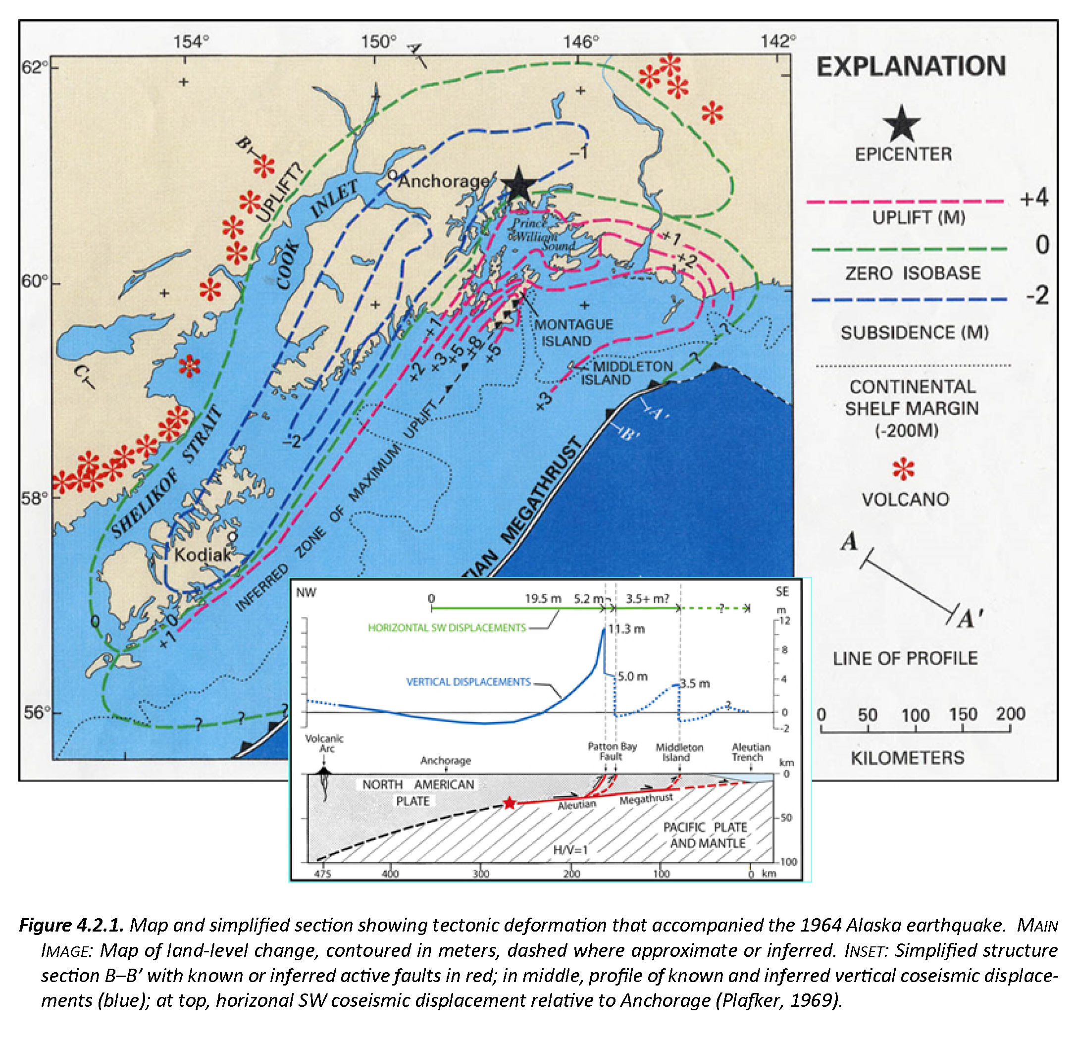
This is a map from Haeussler et al. (2014). The region in red shows the area that subsided and the area in blue shows the region that uplifted during the earthquake. These regions were originally measured in the field by George Plafker and published in several documents, including this USGS Professional Paper (Plafker, 1969).
Here is a cross section showing the differences of vertical deformation between the coseismic (during the earthquake) and interseismic (between earthquakes).
This figure, from Atwater et al. (2005) shows the earthquake deformation cycle and includes the aspect that the uplift deformation of the seafloor can cause a tsunami.
Here is a figure recently published in the 5th International Conference of IGCP 588 by the Division of Geological and Geophysical Surveys, Dept. of Natural Resources, State of Alaska (State of Alaska, 2015). This is derived from a figure published originally by Plafker (1969). There is a cross section included that shows how the slip was distributed along upper plate faults (e.g. the Patton Bay and Middleton Island faults).
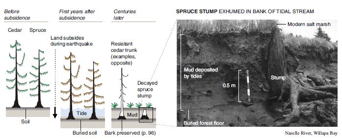
Here is a graphic showing the sediment-stratigraphic evidence of earthquakes in Cascadia, but the analogy works for Alaska also. Atwater et al., 2005. There are 3 panels on the left, showing times of (1) prior to earthquake, (2) several years following the earthquake, and (3) centuries after the earthquake. Before the earthquake, the ground is sufficiently above sea level that trees can grow without fear of being inundated with salt water. During the earthquake, the ground subsides (lowers) so that the area is now inundated during high tides. The salt water kills the trees and other plants. Tidal sediment (like mud) starts to be deposited above the pre-earthquake ground surface. This sediment has organisms within it that reflect the tidal environment. Eventually, the sediment builds up and the crust deforms interseismically until the ground surface is again above sea level. Now plants that can survive in this environment start growing again. There are stumps and tree snags that were rooted in the pre-earthquake soil that can be used to estimate the age of the earthquake using radiocarbon age determinations. The tree snags form “ghost forests.
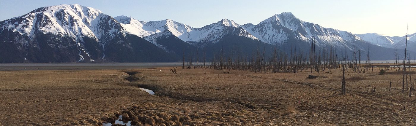
This is a photo that I took along the Seward HWY 1, that runs east of Anchorage along the Turnagain Arm. I attended the 2014 Seismological Society of America Meeting that was located in Anchorage to commemorate the anniversary of the Good Friday Earthquake. This is a ghost forest of trees that perished as a result of coseismic subsidence during the earthquake. Copyright Jason R. Patton (2014). This region subsided coseismically during the 1964 earthquake. Here are some photos from the paleoseismology field trip. (Please contact me for a higher resolution version of this image: quakejay at gmail.com)
This is another video about the 1964 Good Friday Earthquake and how we learned about what happened.
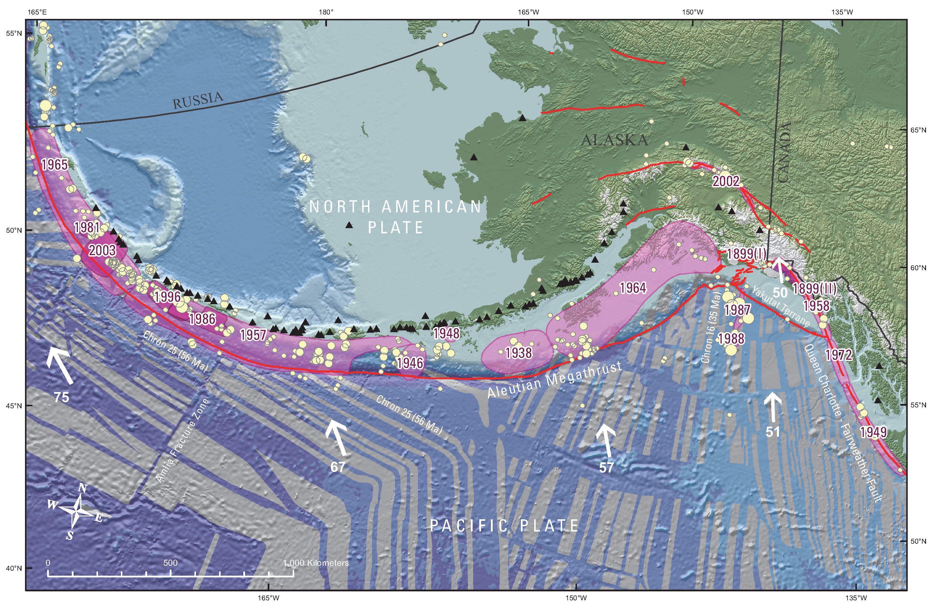
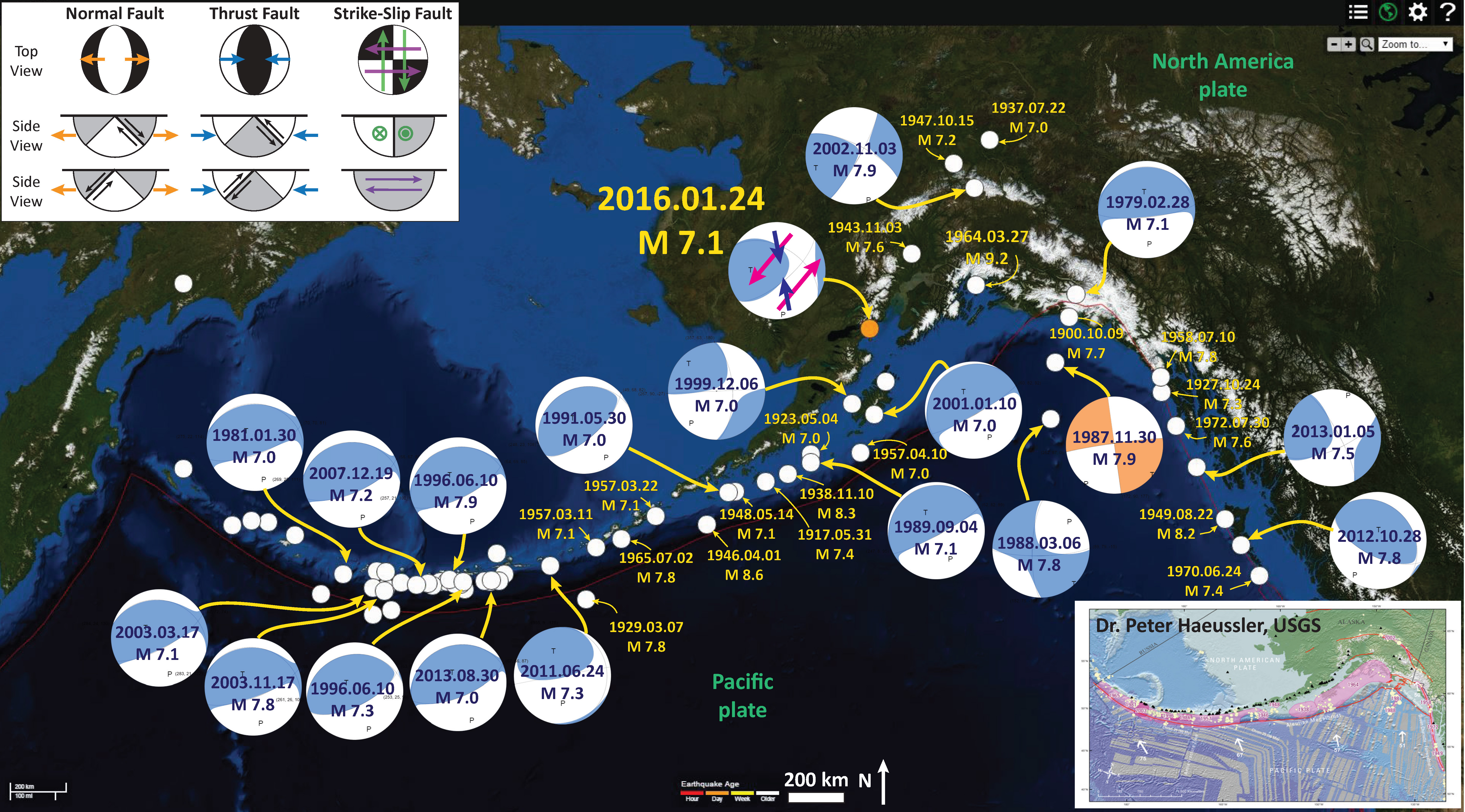
- Here is a map that shows historic earthquake slip regions as pink polygons (Peter Haeussler, USGS). Dr. Haeussler also plotted the magnetic anomalies (grey regions), the arc volcanoes (black diamonds), and the plate motion vectors (mm/yr, NAP vs PP).
- Here is the figure from Sykes et al. (1980) that shows the space time relations for historic earthquakes in relation to the map.

Above: Rupture zones of earthquakes of magnitude M > 7.4 from 1925-1971 as delineated by their aftershocks along plate boundary in Aleutians, southern Alaska and offshore British Columbia [after Sykes, 1971]. Contours in fathoms. Various symbols denote individual aftershock sequences as follows: crosses, 1949, 1957 and 1964; squares, 1938, 1958 and 1965; open triangles, 1946; solid triangles, 1948; solid circles, 1929, 1972. Larger symbols denote more precise locations. C = Chirikof Island. Below: Space-time diagram showing lengths of rupture zones, magnitudes [Richter, 1958; Kanamori, 1977 b; Kondorskay and Shebalin, 1977; Kanamori and Abe, 1979; Perez and Jacob, 1980] and locations of mainshocks for known events of M > 7.4 from 1784 to 1980. Dashes denote uncertainties in size of rupture zones. Magnitudes pertain to surface wave scale, M unless otherwise indicated. M is ultra-long period magnitude of Kanamori 1977 b; Mt is tsunami magnitude of Abe[ 1979]. Large shocks 1929 and 1965 that involve normal faulting in trench and were not located along plate interface are omitted. Absence of shocks before 1898 along several portions of plate boundary reflects lack of an historic record of earthquakes for those areas.
- Here is a great illustration that shows how forearc sliver faults form due to oblique convergence at a subduction zone (Lange et al., 2008). Strain is partitioned into fault normal faults (the subduction zone) and fault parallel faults (the forearc sliver faults, which are strike-slip). This figure is for southern Chile, but is applicable globally.

Proposed tectonic model for southern Chile. Partitioning of the oblique convergence vector between the Nazca plate and South American plate results in a dextral strike-slip fault zone in the magmatic arc and a northward moving forearc sliver. Modified after Lavenu and Cembrano (1999).
In 2016, there was an earthquake along the Alaska Peninsula, a M 7.1 on 2016.01.24. Here is my earthquake report for this earthquake. Here is a map for the earthquakes of magnitude greater than or equal to M 7.0 between 1900 and today. This is the USGS query that I used to make this map. One may locate the USGS web pages for all the earthquakes on this map by following that link.
Some Relevant Discussion and Figures
- Johnson and Satake (1994) studied tsunami waveforms from the 10 November 1938 Alaska M 8.2 earthquake. Their analysis was designed to estimate the source for the tsunami. Below are some figures from their paper, with figure captions beneath each figure.
- This first plot shows the tsunami records from tide gages. This is the plot I used to consider the potential impact to the coast from the 2021 M 8.2 tsunami.
- Here is a map that shows the fault model that they used, as well as the amount of slip that they used for each fault element.
- This is a figure comparing their model results (synthetic = dashed) compared to the tide gage records (solid lines).
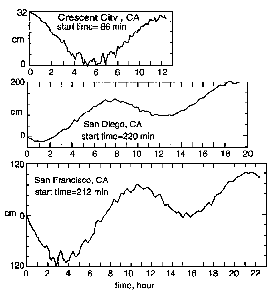
Digitized marigrams from 1938 Alaskan earthquake recorded in Crescent City, San Diego, and San Francisco. The tidal componenht asn ot beenr emoved.S tartt ime listedf or each record is the time in minutes from the origin time of the earthquaketo the startt ime of the digitizedr ecord.
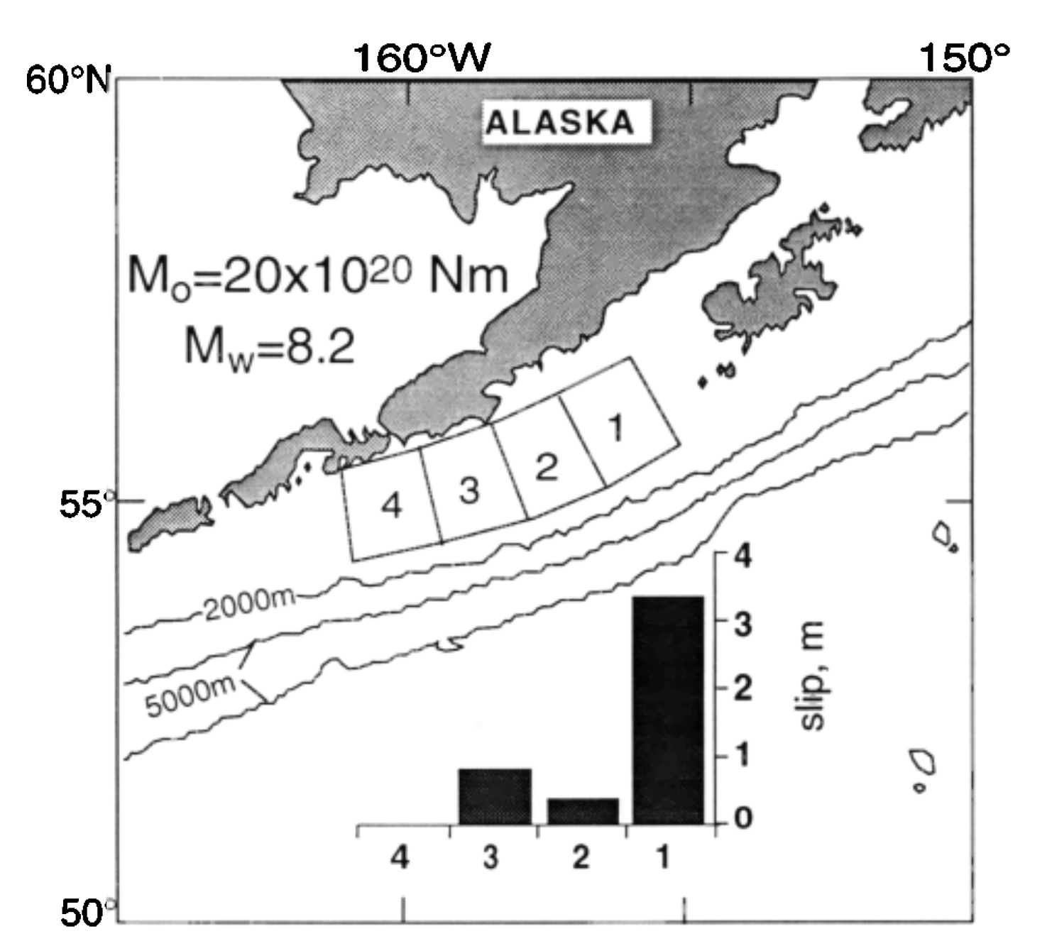
Location of subfaults used in inversion of tsunami waveforms. Graph shows slip distribution in meters.

Observed and synthetic waveforms from inversion for four subfaults. Start time of each record is different. The arrows indicate the parts of the waveforms used for the inversion.
- Freymueller et al. (2021) also studied the 1938 M 8.2 event, seeking to resolve the slip on the fault using tsunami modeling.
- Below are figures with their captions in blockquote.
- Here are some maps showing 2 of the slip distrubutions that they used for their modeling.
- Here are some maps showing vertical seafloor displacements for some of their tsunami scenarios.
- Here are plots that show some results of their modeling. The tide gage data are plotted in black and their simulated waves are plotted with red and blue lines.
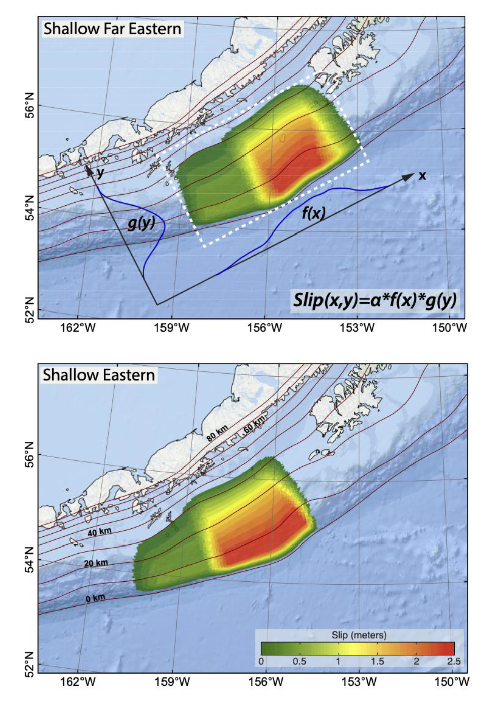
Example slip distributions for two of the slip models, shallow eastern and shallow far eastern. For each model the slip is the product of a function f(x) representing the along-strike variation and g(y) representing the downdip variation, and then scaled to a constant magnitude MW 8.25. The functions f(x) and g(y) are based on relations in Freund and Barnett [1976]. For the central and western models, the rupture area is the same as for the eastern model, but the area of higher slip is shifted to the west. For the mid-depth and deep models, the main area of high slip is shifted downdip.
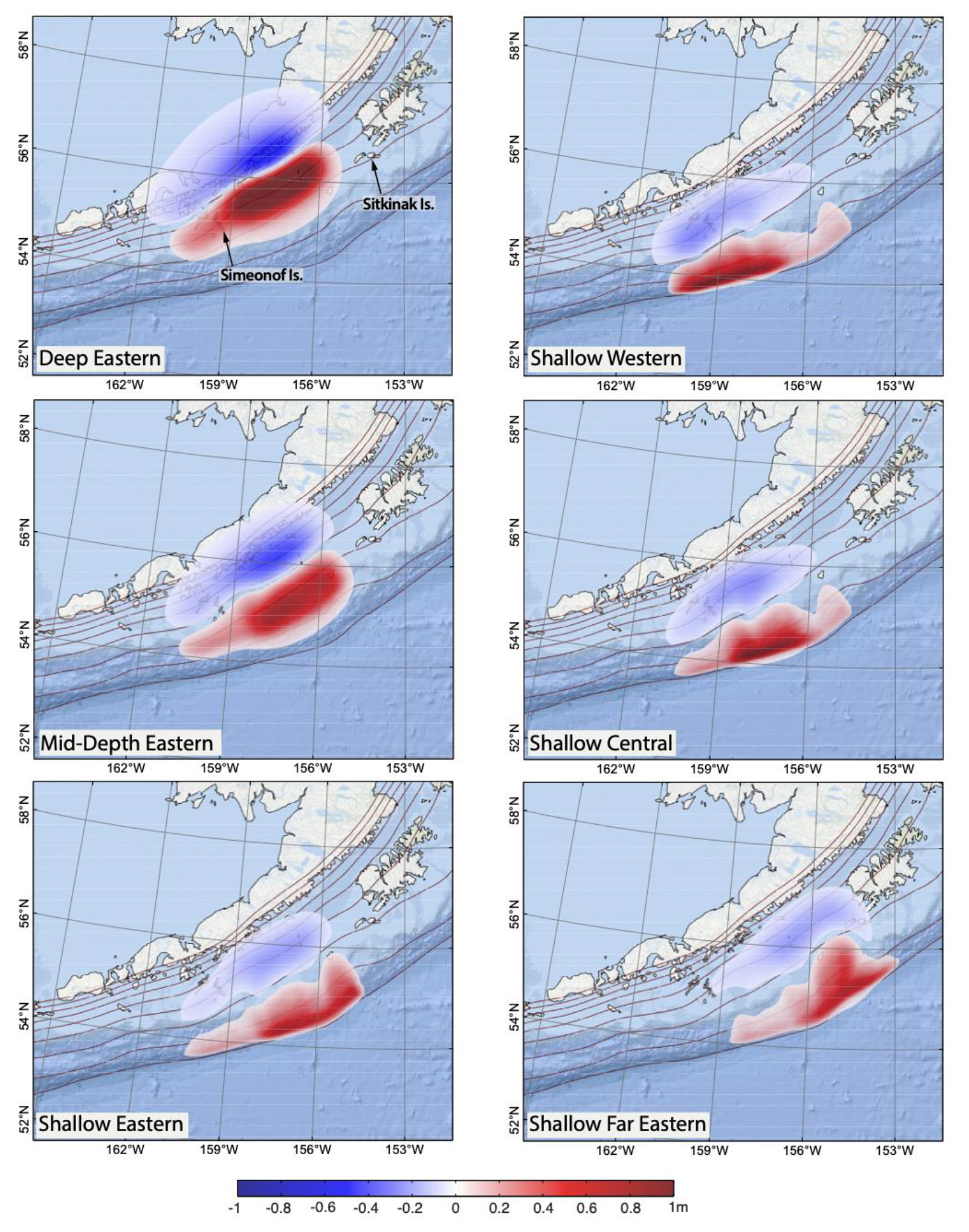
Vertical seafloor displacements caused by representative slip scenarios. On the left side, the slip is concentrated in the east and the deep, mid-depth and shallow slip distribution scenarios are shown. On the right, the Western, Central and Far Eastern slip distribution scenarios are shown assuming the shallow rupture. Displacements are in meters. Red contours show depth to the plate interface from 0 to 80 km with a 10 km increment.
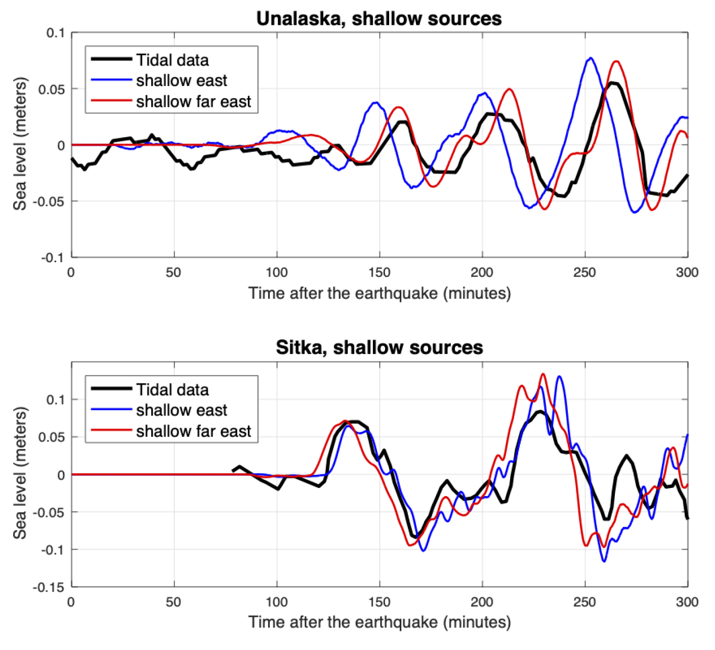
Tide gauge data and model predictions for the eastern and far eastern source models.
Here is an animation from one of the Freymueller et al. (2021) models for the 1938 M 8.2 tsunami.
- Nelson et al. (2015) presented their evidence for prehistoric tsunami on Chirikof Island, an island in the forearc in the eastern part of the 1938 earthquake slip patch.
- They found evidence for many tsunami over a timespan from before 5000 years ago.
- Below are some figures from their paper, with figure captions in blockquote.
- This figure shows the tectonic setting and the area of their field study.
- Here is a plot that shows the timing for the prehistoric tsunami inferred by these authors. The vertical axis is the time scale, with “today” at the top. Each colored pattern represents the age range for a tsunami deposit.
- These data are plotted left to right, west to east, so we can compare tsunami records at different locations along the margin. These comparisons are important so that we can test different hypotheses about how subduciton faults may slip over time. In the 2021 case, the slip area was close to the 1938 earthquake. But, did has this always occured here?
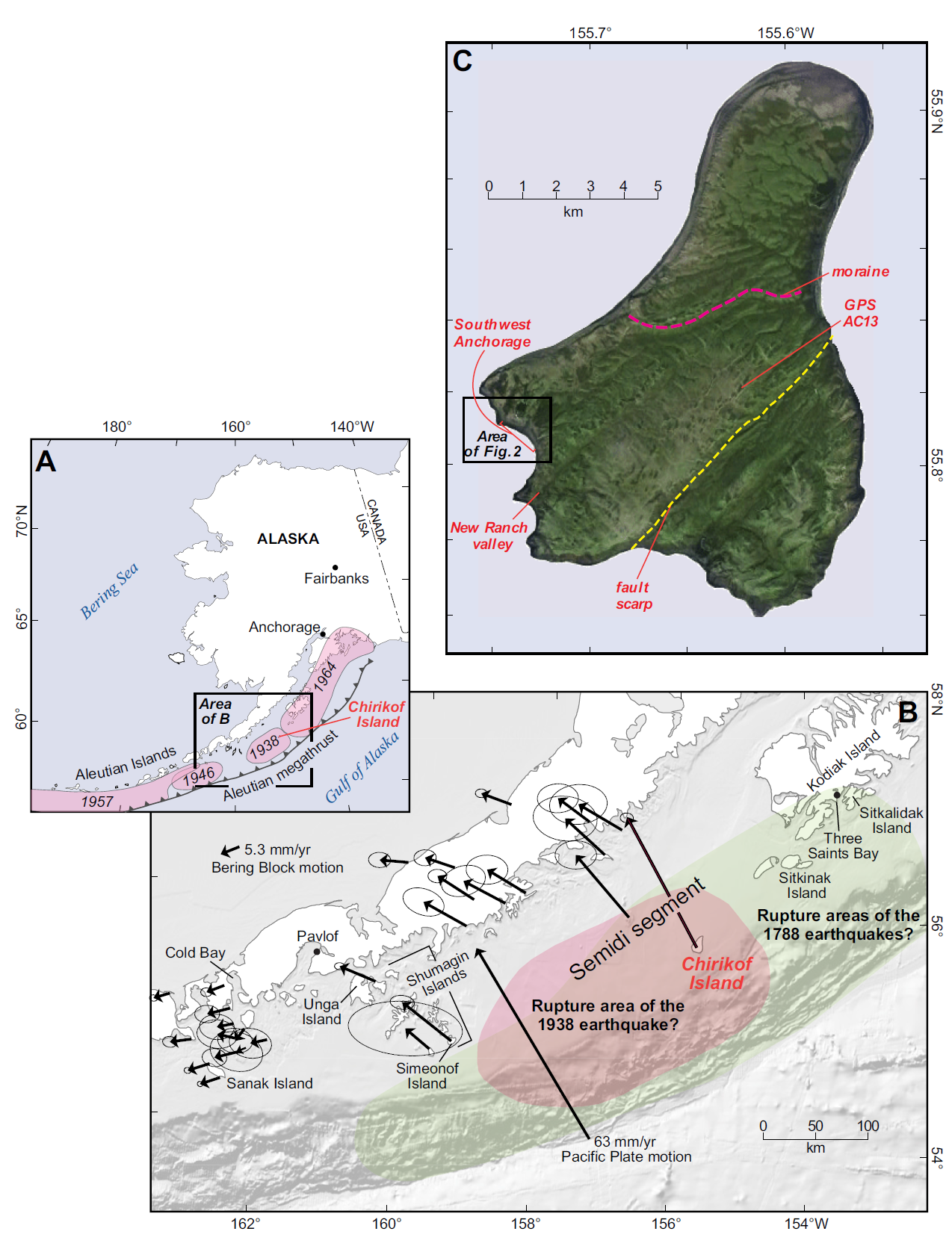
A) Location of Chirikof Island within the plate tectonic setting of the Alaska-Aleutian subduction zone. Rupture areas for great twentieth century earthquakes on the megathrust are in pink. (B) Velocity field of the Alaska Peninsula and the eastern Aleutian Islands observed by global positioning system (GPS) (Fournier and Freymueller, 2007). Colors show inferred rupture areas for earthquakes in 1788 (green) and 1938 (orange). Both A and B are modified from Witter et al. (2014). The section of the megathrust between Kodiak Island and the Shumagin Islands has been referred to as the Semidi segment (e.g., Shennan et al., 2014b). (C) Physiography of Chirikof Island (Google Earth image, 2012) showing the location of our study area at Southwest Anchorage, a prominent moraine, a fault scarp (facing southeast) that probably records the 1880 earthquake, the New Ranch valley reconnaissance core site, and UNAVCO GPS station AC13 (http:// pbo .unavco .org /station /overview /AC13). In the eighteenth and nineteenth centuries, Chirikof Island was known to native Alutiiq and Russians as Ukamuk Island.
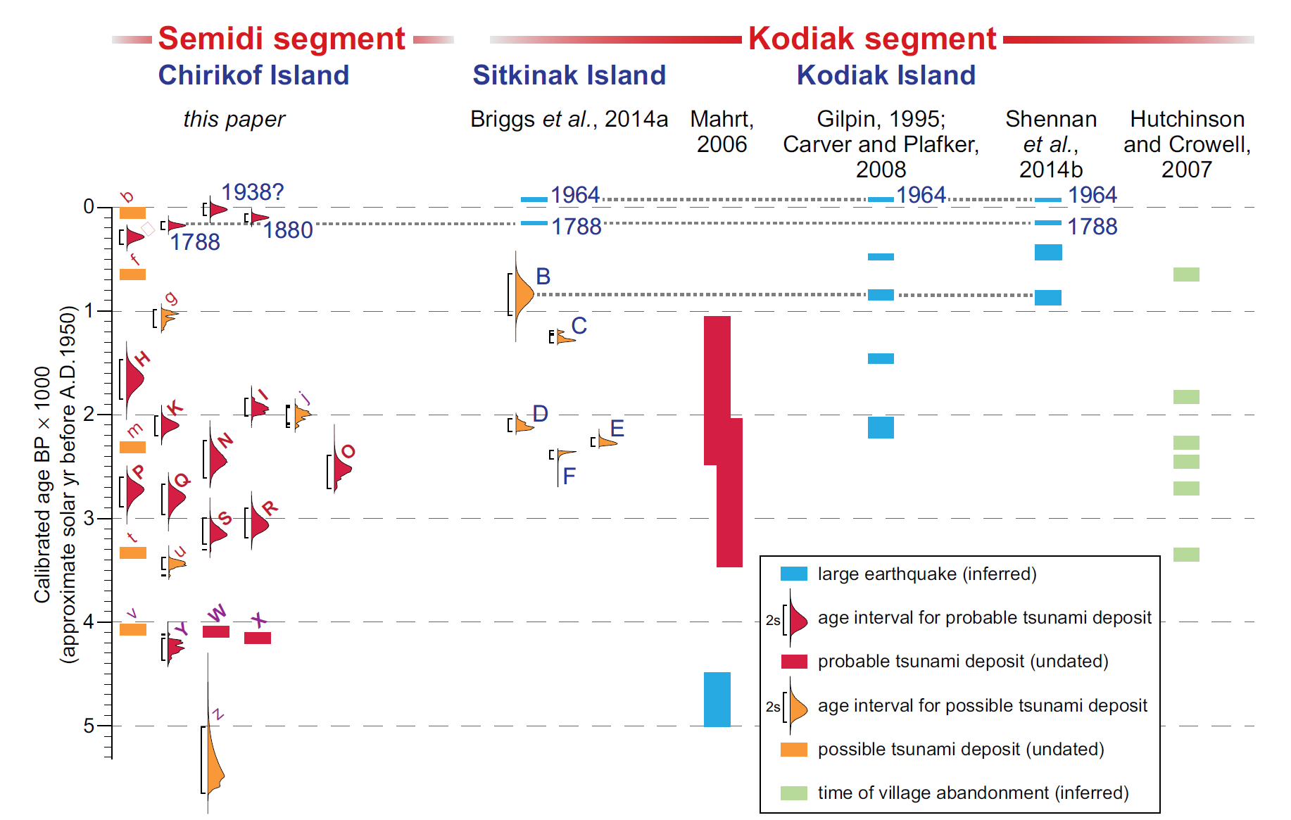
Age probability distributions for probable (red) and possible (orange) tsunami deposits at Southwest Anchorage (labels as in Fig. 11) compared with age distributions for possible tsunami deposits at Sitkinak Island (Briggs et al., 2014a) and with age estimates for great earthquakes and tsunamis on Kodiak Island (from studies referenced on this figure;
Fig. 1). Dotted horizontal lines show our correlation of evidence for some younger earthquakes and tsunamis. Times of great earthquakes inferred from episodes of village abandonment determined from archaeological stratigraphy in the eastern Alaska-Aleutian megathrust region are also shown (Hutchinson and Crowell, 2007).
Social Media
#EarthquakeReport for M7.3 #Earthquake offshore of #SandPoint #Alaska
Right-lateral (?) Strike-slip earthquake mechanism
within subducting Pacific plate
Maybe small local #Tsunami (?)Earthquake in similar location in 2023 https://t.co/4ZLXRvjvrXhttps://t.co/2iUwo8xtEp pic.twitter.com/WN1eWMWsFl
— Jason "Jay" R. Patton (@patton_cascadia) July 16, 2025
#EarthquakeReport for M 7.3 #Earthquake offshore of #Alaska
generated small #Tsunami ~10 cm amplitude at Sand Point
right-lateral strike-slip mechanism
intraplate earthquake in upper North America plate ~10km above slab 2 depthread report:https://t.co/jjtENAtEMq pic.twitter.com/bACSgi88dx
— Jason "Jay" R. Patton (@patton_cascadia) July 19, 2025
From the National Tsunami Warning Center:
🔴 A TSUNAMI WARNING is posted for portions of Alaska following a M7.2 earthquake 50 miles S of Sand Point, Alaska, at 12:38pm AKDT July 16.
A Tsunami Alert is for this event is posted at https://t.co/npoUHxWBas
— NWS Tsunami Alerts (@NWS_NTWC) July 16, 2025
CANCELLATION: M7.3 055mi S Sand Point, Alaska 1238AKDT Jul 16: Check with local officials for all clear
— NWS Tsunami Alerts (@NWS_NTWC) July 16, 2025
Here's a quick overview of today's magnitude 7.3 earthquake near Sand Point, including aftershocks and some context for this region that has seen four other earthquakes over magnitude seven in the past 5 years. https://t.co/p3Zaw5BEZy
— Alaska Earthquake Center (@AKearthquake) July 17, 2025
Here at the Alaska Earthquake Center we've been busy fielding inquiries into the magnitude 7.3 earthquake south of Sand Point, AK that occurred around 12:40 pm today. Here, AEC Director and State Seismologist Michael West describes what we know so far. Follow along as we update… pic.twitter.com/49ZlcFMeKt
— Alaska Earthquake Center (@AKearthquake) July 17, 2025
Yesterday's magnitude 7.3 earthquake, which we have dubbed "2025 Sand Point Earthquake," has attracted a bit of media attention. This story posted today has some good overview content and a new graphic we created to show the location and context of the event and its aftershocks… pic.twitter.com/AshVaIEnK9
— Alaska Earthquake Center (@AKearthquake) July 18, 2025
Mistake in labels of P, S, and Surface Waves: This one is fixed. pic.twitter.com/lo6I4jh9Y9
— Alan Kafka (@Weston_Quakes) July 17, 2025
Security cameras captured a powerful 7.3 magnitude earthquake rocking a home in Sand Point, Alaska, this week. The earthquake prompted a tsunami warning and evacuations in the area. pic.twitter.com/GRrGknib3O
— AccuWeather (@accuweather) July 18, 2025
- Summary of the 1964 Earthquake
- 2025.07.16 M 7.3 Alaska
- 2024.08.17 M 7.0 Kamchatka
- 2023.07.16 M 7.2 Alaska POSTER
- 2021.07.29 M 8.2 Alaska
- 2020.10.19 M 7.5 Alaska POSTER
- 2020.07.22 M 7.8 Alaska POSTER
- 2019.04.02 M 6.5 Aleutians
- 2019.03.26 M 5.2 Alaska
- 2018.12.20 M 7.4 Bering Kresla
- 2018.12.20 M 7.3 Bering Kresla UPDATE #1
- 2018.11.30 M 7.0 Alaska
- 2018.08.15 M 6.6 Aleutians
- 2018.08.12 M 6.4 North Alaska
- 2018.08.12 M 6.4 North Alaska UPDATE #1
- 2018.01.23 M 7.9 Gulf of Alaska
- 2018.01.23 M 7.9 Gulf of Alaska UPDATE #1
- 2018.01.23 M 7.9 Gulf of Alaska UPDATE #2
- 2017.07.17 M 7.7 Aleutians
- 2017.07.17 M 7.7 Aleutians UPDATE #1
- 2017.06.02 M 6.8 Aleutians
- 2017.05.08 M 6.2 Aleutians
- 2017.05.01 M 6.3 British Columbia
- 2017.03.29 M 6.6 Kamchatka
- 2017.03.02 M 5.5 Alaska
- 2016.09.05 M 6.3 Bering Kresla (west of Aleutians)
- 2016.04.13 M 5.7 & 6.4 Kamchatka
- 2016.04.02 M 6.2 Alaska Peninsula
- 2016.03.27 M 5.7 Aleutians
- 2016.03.12 M 6.3 Aleutians
- 2016.01.29 M 7.2 Kamchatka
- 2016.01.24 M 7.1 Alaska
- 2015.11.09 M 6.2 Aleutians
- 2015.11.02 M 5.9 Aleutians
- 2015.11.02 M 5.9 Aleutians (update)
- 2015.07.27 M 6.9 Aleutians
- 2015.05.29 M 6.7 Alaska Peninsula
- 2015.05.29 M 6.7 Alaska Peninsula (animations)
- 1964.03.27 M 9.2 Good Friday
Alaska | Kamchatka | Kurile
General Overview
Earthquake Reports
- Frisch, W., Meschede, M., Blakey, R., 2011. Plate Tectonics, Springer-Verlag, London, 213 pp.
- Hayes, G., 2018, Slab2 – A Comprehensive Subduction Zone Geometry Model: U.S. Geological Survey data release, https://doi.org/10.5066/F7PV6JNV.
- Holt, W. E., C. Kreemer, A. J. Haines, L. Estey, C. Meertens, G. Blewitt, and D. Lavallee (2005), Project helps constrain continental dynamics and seismic hazards, Eos Trans. AGU, 86(41), 383–387, , https://doi.org/10.1029/2005EO410002. /li>
- Jessee, M.A.N., Hamburger, M. W., Allstadt, K., Wald, D. J., Robeson, S. M., Tanyas, H., et al. (2018). A global empirical model for near-real-time assessment of seismically induced landslides. Journal of Geophysical Research: Earth Surface, 123, 1835–1859. https://doi.org/10.1029/2017JF004494
- Kreemer, C., J. Haines, W. Holt, G. Blewitt, and D. Lavallee (2000), On the determination of a global strain rate model, Geophys. J. Int., 52(10), 765–770.
- Kreemer, C., W. E. Holt, and A. J. Haines (2003), An integrated global model of present-day plate motions and plate boundary deformation, Geophys. J. Int., 154(1), 8–34, , https://doi.org/10.1046/j.1365-246X.2003.01917.x.
- Kreemer, C., G. Blewitt, E.C. Klein, 2014. A geodetic plate motion and Global Strain Rate Model in Geochemistry, Geophysics, Geosystems, v. 15, p. 3849-3889, https://doi.org/10.1002/2014GC005407.
- Meyer, B., Saltus, R., Chulliat, a., 2017. EMAG2: Earth Magnetic Anomaly Grid (2-arc-minute resolution) Version 3. National Centers for Environmental Information, NOAA. Model. https://doi.org/10.7289/V5H70CVX
- Müller, R.D., Sdrolias, M., Gaina, C. and Roest, W.R., 2008, Age spreading rates and spreading asymmetry of the world’s ocean crust in Geochemistry, Geophysics, Geosystems, 9, Q04006, https://doi.org/10.1029/2007GC001743
- Pagani,M. , J. Garcia-Pelaez, R. Gee, K. Johnson, V. Poggi, R. Styron, G. Weatherill, M. Simionato, D. Viganò, L. Danciu, D. Monelli (2018). Global Earthquake Model (GEM) Seismic Hazard Map (version 2018.1 – December 2018), DOI: 10.13117/GEM-GLOBAL-SEISMIC-HAZARD-MAP-2018.1
- Silva, V ., D Amo-Oduro, A Calderon, J Dabbeek, V Despotaki, L Martins, A Rao, M Simionato, D Viganò, C Yepes, A Acevedo, N Horspool, H Crowley, K Jaiswal, M Journeay, M Pittore, 2018. Global Earthquake Model (GEM) Seismic Risk Map (version 2018.1). https://doi.org/10.13117/GEM-GLOBAL-SEISMIC-RISK-MAP-2018.1
- Zhu, J., Baise, L. G., Thompson, E. M., 2017, An Updated Geospatial Liquefaction Model for Global Application, Bulletin of the Seismological Society of America, 107, p 1365-1385, https://doi.org/0.1785/0120160198
- Abe, K., 1972. Lithospheric Normal Faulting Beneath the Aleutian Trench in Phys. Earth Planet. Interiors, v. 5, p. 1990-198.
- Atwater, B.F., Yamaguchi, D.K., Bondevik, S., Barnhardt, W.A., Amidon, L.J., Benson, B.E., Skjerdal, G., Shulene, J.A., and Nanalyama ,F., 2001. Rapid resetting of an estuarine recorder of the 1964 Alaska earthquake in Geology, v. 113, no. 9, p. 1193-1204.
- Bassett and Watts, 2015 A. Gravity anomalies, crustal structure, and seismicity at subduction zones: 1. Seafloor roughness and subducting relief in Geochemistry, Geophysics, Geosystems, v. 16, doi:10.1002/2014GC005684.
- Bassett, D. and Watts, A.B., 2015 B. Gravity anomalies, crustal structure, and seismicity at subduction zones: 2. Interrelationships between fore-arc structure and seismogenic behavior in Geochemistry, Geophysics, Geosystems, v. 16, doi:10.1002/2014GC005685.
- Benz, H.M., Tarr, A.C., Hayes, G.P., Villaseñor, Antonio, Hayes, G.P., Furlong, K.P., Dart, R.L., and Rhea, Susan, 2011. Seismicity of the Earth 1900–2010 Aleutian arc and vicinity: U.S. Geological Survey Open-File Report 2010–1083-B, scale 1:5,000,000.
- Brown, J.R., Prejan, S.G., Beroza, G.C., Gomberg, J.S., and Hauessler,m P.J., 2013. Deep low-frequency earthquakes in tectonic tremor along the Alaska-Aleutian subduction zone in JGR Solid Earth, v. 118, p. 1079-1090, doi:10.1029/2012JB009459
- Freymueller, J.T., Suleimani, E.N., and Nocolski, D.J., 2021. Constraints on the Slip Distribution of the 1938 MW 8.3 Alaska Peninsula Earthquake From Tsunami Modeling in GRL, v. 48, no. 9, https://doi.org/10.1029/2021GL092812
- Frisch, W., Meschede, M., Blakey, R., 2011. Plate Tectonics, Springer-Verlag, London, 213 pp.
- Gaedicke, C., Baranov, B., Seliverstov, N., Alexeiev, D., Tsukanov, N., Freitag, R., 2000. Structure of an active arc-continent collision area: the Aleutian-Kamchatka junction. Tectonophysics 325, 63–85
- Haeussler, P., Leith, W., Wald, D., Filson, J., Wolfe, C., and Applegate, D., 2014. Geophysical Advances Triggered by the 1964 Great Alaska Earthquake in EOS, Transactions, American Geophysical Union, v. 95, no. 17, p. 141-142.
- Hayes, G. P., D. J. Wald, and R. L. Johnson, 2012. Slab1.0: A three-dimensional model of global subduction zone geometries, J. Geophys. Res., 117, B01302, doi:10.1029/2011JB008524.
- Ikuta, R., Mitsui, Y., Kurokawa, Y., and Ando, M., 2015. Evaluation of strain accumulation in global subduction zones from seismicity data in Earth, Planets and Space, v. 67, DOI 10.1186/s40623-015-0361-5
- Johnson, J.M. and Satake, K., 1994. Rupture extent of the 1938 Alaskan earthquake as inferred from tsunami waveforms in GRL, v. 21, no. 8, p. 733-736
- Koulakov, I.Y., Dobretsov, N.L., Bushenkova, N.A., and Yakovlev, A.V., 2011. Slab shape in subduction zones beneath the Kurile–Kamchatka and Aleutian arcs based on regional tomography results in Russian Geology and Geophysics, v. 52, p. 650-667.
- Konstantnovskaia, 2001. Arc-continent collision and subduction reversal in the Cenozoic evolution of the Northwest Pacific: an example from Kamchatka (NE Russia) in Tectonophysics, v. 333, p. 75-94.
- Krutikov, L., Stone, D.B., and Minyuk, P., 2008. New Paleomagnetic Data From the Central Aleutian Arc: Evidence and Implications for Block Rotations in Active Tectonics and Seismic Potential of Alaska, Geophysical Monograph Series 179 American Geophysical Union. 10.1029/179GM07
- Lange, D., Cembrano, J., Rietbrock, A., Haberland, C., Dahm, T., and Bataille, K., 2008. First seismic record for intra-arc strike-slip tectonics along the Liquiñe-Ofqui fault zone at the obliquely convergent plate margin of the southern Andes in Tectonophysics, v. 455, p. 14-24
- Lay, T., H. Kanamori, C. J. Ammon, A. R. Hutko, K. Furlong, and L. Rivera, 2009. The 2006 – 2007 Kuril Islands great earthquake sequence in J. Geophys. Res., 114, B11308, doi:10.1029/2008JB006280.
- Lay, T., Ye, L., Bai, Y., Cheung, K. F., Kanamori, H., Freymueller, J., … Kogan, M. G. (2017). Rupture along 400 km of the Bering fracture zone in the Komandorsky Islands earthquake (MW 7.8) of 17 July 2017. Geophysical Research Letters, 44, 12,161–12,169. https://doi.org/10.1002/2017GL076148
- Meyer, B., Saltus, R., Chulliat, a., 2017. EMAG2: Earth Magnetic Anomaly Grid (2-arc-minute resolution) Version 3. National Centers for Environmental Information, NOAA. Model. https://doi.org/10.7289/V5H70CVX
- Müller, R.D., Sdrolias, M., Gaina, C. and Roest, W.R., 2008, Age spreading rates and spreading asymmetry of the world’s ocean crust in Geochemistry, Geophysics, Geosystems, 9, Q04006, https://doi.org/10.1029/2007GC001743
- Nelson, A.R., Briggs, R.W., Dura, T., Engelhart, S.E., Gelfenbaum, G., Bradley, L.-A., Forman, S.L., Vane, C.H., and Kelley, K.A., 2015, Tsunami recurrence in the eastern Alaska-Aleutian arc: A Holocene stratigraphic record from Chirikof Island, Alaska: Geosphere, v. 11, no. 4, p. 1172–1203, doi:10.1130/GES01108.1.
- Plafker, G., 1969. Tectonics of the March 27, 1964 Alaska earthquake: U.S. Geological Survey Professional Paper 543–I, 74 p., 2 sheets, scales 1:2,000,000 and 1:500,000, http://pubs.usgs.gov/pp/0543i/.
- Plafker, G., 1972. Alaskan earthquake of 1964 and Chilean earthquake of 1960: Implications for arc tectonics in Journal of Geophysical Research, v. 77, p. 901-925.
- Portnyagin, M. and Manea, V.C., 2008. Mantle temperature control on composition of arc magmas along the Central Kamchatka Depression in Geology, v. 36, no. 7, p. 519-522.
- Rhea, S., Tarr, A.C., Hayes, G., Villaseñor, A., Furlong, K.P., and Benz, H.M., 2010. Seismicity of the Earth 1900-2007, Kuril-Kamchatka arc and vicinity: U.S. Geological Survey Open-File Report 2010-1083-C, 1 map sheet, scale 1:5,000,000.
- Saltus, R.W., and Barnett, A., 2000. Eastern Aleutian Volcanic Arc Digital Model – Version 1.0: U.S. Geological Survey Open-File Report 00
- Shevchenko, V.I., Lukk, A.A., and Prilepin, M.T., 2006. The Sumatra Earthquake of December 26, 2004, as an Event Unrelated to the Plate-Tectonic Process in the Lithosphere in Physics of the Solid Earth, v. 42, no. 12, p. 1018–1037.
- Stauder, W., 1968. Mechanism of the Rat Island Earthquake Sequence of February 4, 1965, with Relation to Island Arcs and Sea-Floor Spreading in JGR, v. 73, no. 12, p. 3847-3858
- Sykes, L.R., Kissinger, J.B>, House, L., Davies, J.N>, and Jacob, K.H., 1980. Rupture Zones and Repeat Times of Great Earthquakes Along the Alaska-Aleutian Arc, 1784-1980, in Maurice Ewing Series, Earthquake Prediction, An International Review, AGU
- Torsvik, T. H. et al., 2017. Pacific plate motion change caused the Hawaiian-Emperor Bend in Nat. Commun., v. 8, doi: 10.1038/ncomms15660
- Wilson, J. Tuzo, 1963. “A possible origin of the Hawaiian Islands” in Canadian Journal of Physics. v. 41, p. 863–870 doi:10.1139/p63-094.
References:
Basic & General References
Specific References
Return to the Earthquake Reports page.
- Sorted by Magnitude
- Sorted by Year
- Sorted by Day of the Year
- Sorted By Region