Well, the USGS updated their earthquake mechanism (moment tensor) to be more steeply dipping, showing a more vertical fault possibly. This makes more sense given the historic earthquakes in this region and our knowledge of the history of this complicated plate boundary. The USGS also updated their model of shaking intensity (MMI) and revised the magnitude to M =7.3 (though I keep M = 7.4 in these reports to avoid confusion).
I present a larger scale map with more historic earthquake mechanisms below.
These historic mechanisms reveal something about how the Pacific plate subducts beneath the Okhotsk plate (part of North America). Read more about the tectonics and my initial interpretation of this earthquake in the first earthquake report here.
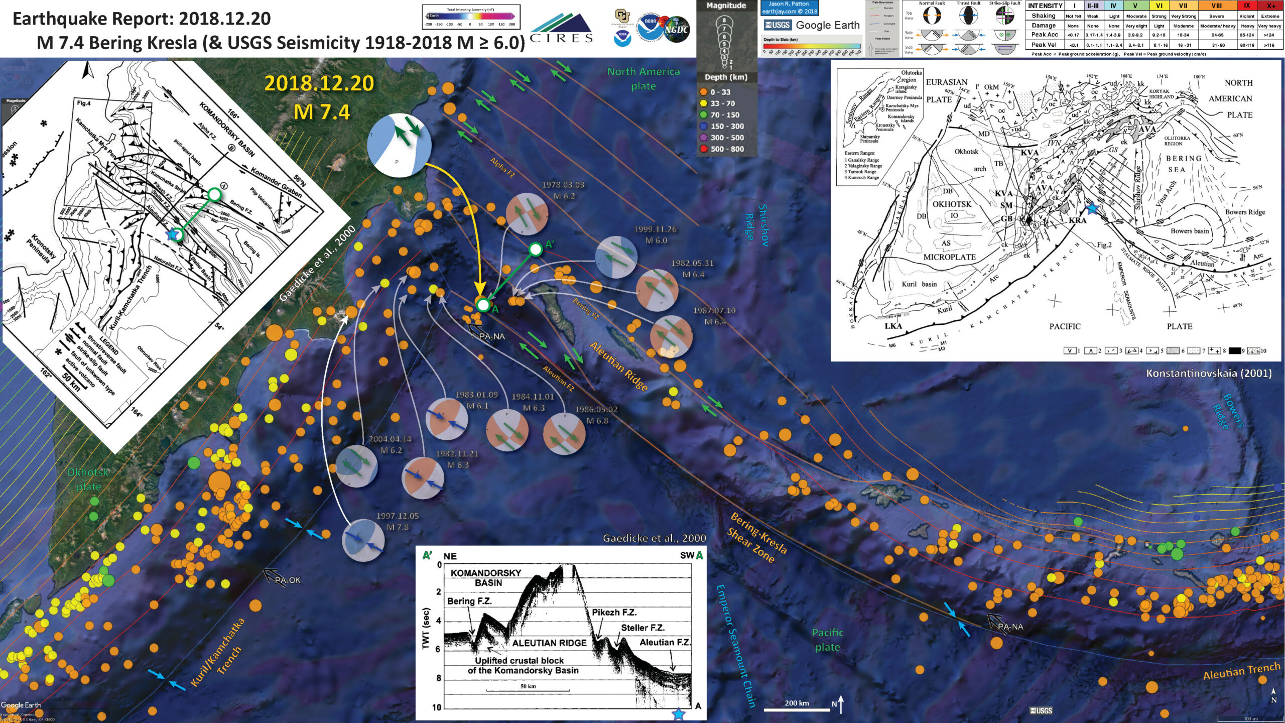
The M = 7.4 earthquake from yesterday clearly ruptured the Aleutian fracture zone (AFZ), which is part of the Bering Kresla Shear zone. There is a series of aftershocks that plot to the southwest of the mainshock, but these are mislocated. The M =7.4 was originally located to the southwest also (off of the fault), but has since been relocated. So, I suspect that these aftershocks could be relocated also, if someone were to work on them (e.g. double difference analysis). The 1978.03.03 M 6.2 earthquake is a great analogy for this M 7.4 as it is in the same location and has a nice right-lateral strike slip focal mechanism.
The relative motion between the Pacific plate and North America plate here is parallel to the plate boundary, giving rise to this shear zone. To the west, the Pacific plate subducts beneath the Okhotsk plate to form the Kuril/Kamchatka trench.
We can see strike slip earthquakes west of the trench (1984.11.01 and 1986.05.02). Further to the west, there are some earthquakes that show the convergence associated with this subduction margin (1983.01.09, 1982.11.21, 1997.12.05). The Aleutian fracture zone exists within the Pacific plate as it dives beneath the Okhotsk plate,as evidenced by the 2004.04.14 M = 6.2 earthquake.
Below is my interpretive poster for this earthquake
I plot the seismicity from the past month, with color representing depth and diameter representing magnitude (see legend). I include earthquake epicenters from 1918-2018 with magnitudes M ≥ 6.0 in one version.
I plot the USGS fault plane solutions (moment tensors in blue and focal mechanisms in orange), possibly in addition to some relevant historic earthquakes.
- I placed a moment tensor / focal mechanism legend on the poster. There is more material from the USGS web sites about moment tensors and focal mechanisms (the beach ball symbols). Both moment tensors and focal mechanisms are solutions to seismologic data that reveal two possible interpretations for fault orientation and sense of motion. One must use other information, like the regional tectonics, to interpret which of the two possibilities is more likely.
- I also include the shaking intensity contours on the map. These use the Modified Mercalli Intensity Scale (MMI; see the legend on the map). This is based upon a computer model estimate of ground motions, different from the “Did You Feel It?” estimate of ground motions that is actually based on real observations. The MMI is a qualitative measure of shaking intensity. More on the MMI scale can be found here and here. This is based upon a computer model estimate of ground motions, different from the “Did You Feel It?” estimate of ground motions that is actually based on real observations.
- I include the slab 2.0 contours plotted (Hayes, 2018), which are contours that represent the depth to the subduction zone fault. These are mostly based upon seismicity. The depths of the earthquakes have considerable error and do not all occur along the subduction zone faults, so these slab contours are simply the best estimate for the location of the fault.li>
- In the map below, I include a transparent overlay of the magnetic anomaly data from EMAG2 (Meyer et al., 2017). As oceanic crust is formed, it inherits the magnetic field at the time. At different points through time, the magnetic polarity (north vs. south) flips, the north pole becomes the south pole. These changes in polarity can be seen when measuring the magnetic field above oceanic plates. This is one of the fundamental evidences for plate spreading at oceanic spreading ridges (like the Gorda rise).
- Regions with magnetic fields aligned like today’s magnetic polarity are colored red in the EMAG2 data, while reversed polarity regions are colored blue. Regions of intermediate magnetic field are colored light purple.
Magnetic Anomalies
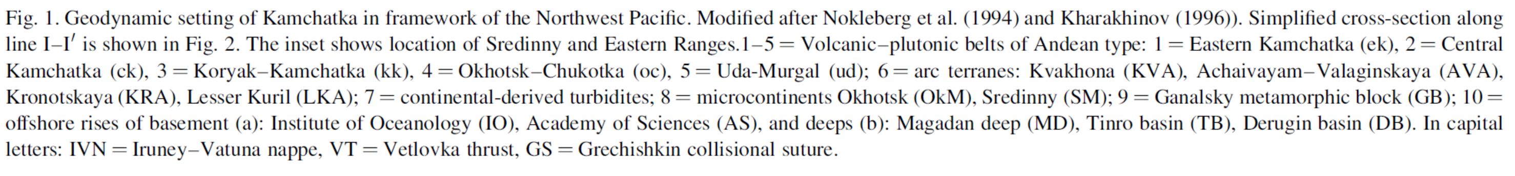
- In the upper right corner I include a map that shows more details about the faulting in the region (Konstantinovskaia (2001).
- In the upper left corner is a map from Gaedicke et a. (2000) that shows a detailed map of the faulting in the region. Note that there are strike-slip, normal, and thrust faults all overlapping in cool ways. When I wrote my intitial report, I hypothesized that the M = 7.4 earthquake was extensional and one of the reasons this may happen here is that there are normal faults (extensional) that form sedimentary basins in this area (e.g. the Steller Basin).
- In the lower center, I present a cross section (seismic reflection data) showing the bathymetry from A-A’ (location shown on upper left map and the main map as a green bar bell line) from Gaedicke et al. (2000). Note the different fracture zones. I place a blue star in the general location of the M = 7.4 earthquake.
I include some inset figures. Some of the same figures are located in different places on the larger scale map below.
- Here is the map with a month’s seismicity plotted.

- Here is the map with a century’s seismicity plotted, with earthquakes M ≥ 6.0.

Some Relevant Discussion and Figures
- Here is the large scale map from Gaedicke et al. (2000). Note that the map in the poster is rotated so that north is up, because in this map, north is not “up.” Note the location of the cross sections A-A’ and B-B’.
- Here are the two cross sections (seismic reflection) showing the topography created by these fracture zones (Gaedicke et al., 2000). The lower cross section shows a basin formed by the transtension (extension associated with a strike-slip fault) along the Bering fracture zone.


- Here is the more detailed tectonic map from Konstantinovskaia et al. (2001).

- This is the cross section associated with the above map, showing subduction at the Kuril/Kamchatka trench.


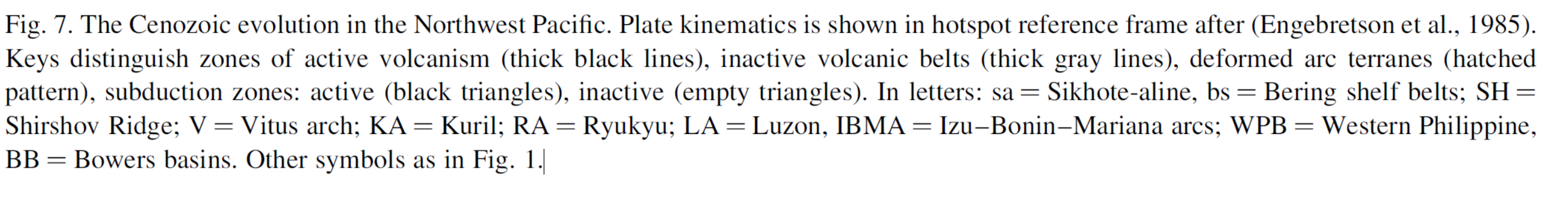
- Below are a series of maps that show the tectonic history in the northwest Pacific. This helps us learn how the plate boundary of the westernmost Aleutian trench is very different from the history of the subduction zone further to the east (responsible for the 1964 Good Friday earthquake for example). The time series begins at the beginning of the Tertiary at about 65 million years ago.


- Finally, here I present tide gage records from the IOC sea level monitoring website. The M = 7.4 earthquake occurred at 2018-12-20 17:01:55 (UTC) and these plots use the UTC time scale. We may observe that there were no tsunami recorded at these gages here and here.


- However, if we take a look at some DART buoy data, we do see some perturbations. Dr. Lori Dengler (emeritus professor at the Humboldt State University, Department of Geology) suggests that these data show surface waves being recorded by these sensors. Below are plots from this buoy. The upper panel are the raw data and the lower panel are the data relative to the prediction.


Geologic Fundamentals
- For more on the graphical representation of moment tensors and focal mechnisms, check this IRIS video out:
- Here is a fantastic infographic from Frisch et al. (2011). This figure shows some examples of earthquakes in different plate tectonic settings, and what their fault plane solutions are. There is a cross section showing these focal mechanisms for a thrust or reverse earthquake. The upper right corner includes my favorite figure of all time. This shows the first motion (up or down) for each of the four quadrants. This figure also shows how the amplitude of the seismic waves are greatest (generally) in the middle of the quadrant and decrease to zero at the nodal planes (the boundary of each quadrant).

- Here is another way to look at these beach balls.
The two beach balls show the stike-slip fault motions for the M6.4 (left) and M6.0 (right) earthquakes. Helena Buurman's primer on reading those symbols is here. pic.twitter.com/aWrrb8I9tj
— AK Earthquake Center (@AKearthquake) August 15, 2018
- There are three types of earthquakes, strike-slip, compressional (reverse or thrust, depending upon the dip of the fault), and extensional (normal). Here is are some animations of these three types of earthquake faults. The following three animations are from IRIS.
Strike Slip:
Compressional:
Extensional:
- This is an image from the USGS that shows how, when an oceanic plate moves over a hotspot, the volcanoes formed over the hotspot form a series of volcanoes that increase in age in the direction of plate motion. The presumption is that the hotspot is stable and stays in one location. Torsvik et al. (2017) use various methods to evaluate why this is a false presumption for the Hawaii Hotspot.
- Here is a map from Torsvik et al. (2017) that shows the age of volcanic rocks at different locations along the Hawaii-Emperor Seamount Chain.

A cutaway view along the Hawaiian island chain showing the inferred mantle plume that has fed the Hawaiian hot spot on the overriding Pacific Plate. The geologic ages of the oldest volcano on each island (Ma = millions of years ago) are progressively older to the northwest, consistent with the hot spot model for the origin of the Hawaiian Ridge-Emperor Seamount Chain. (Modified from image of Joel E. Robinson, USGS, in “This Dynamic Planet” map of Simkin and others, 2006.)

Hawaiian-Emperor Chain. White dots are the locations of radiometrically dated seamounts, atolls and islands, based on compilations of Doubrovine et al. and O’Connor et al. Features encircled with larger white circles are discussed in the text and Fig. 2. Marine gravity anomaly map is from Sandwell and Smith.
- Summary of the 1964 Earthquake
- 2018.12.20 M 7.4 Bering Kresla
- 2018.12.20 M 7.4 Bering Kresla UPDATE #1
- 2018.11.30 M 7.0 Alaska
- 2018.08.15 M 6.6 Aleutians
- 2018.08.12 M 6.4 North Alaska
- 2018.08.12 M 6.4 North Alaska UPDATE #1
- 2018.01.23 M 7.9 Gulf of Alaska
- 2018.01.23 M 7.9 Gulf of Alaska UPDATE #1
- 2018.01.23 M 7.9 Gulf of Alaska UPDATE #2
- 2017.07.17 M 7.7 Aleutians
- 2017.07.17 M 7.7 Aleutians UPDATE #1
- 2017.06.02 M 6.8 Aleutians
- 2017.05.08 M 6.2 Aleutians
- 2017.05.01 M 6.3 British Columbia
- 2017.03.29 M 6.6 Kamchatka
- 2017.03.02 M 5.5 Alaska
- 2016.09.05 M 6.3 Bering Kresla (west of Aleutians)
- 2016.04.13 M 5.7 & 6.4 Kamchatka
- 2016.04.02 M 6.2 Alaska Peninsula
- 2016.03.27 M 5.7 Aleutians
- 2016.03.12 M 6.3 Aleutians
- 2016.01.29 M 7.2 Kamchatka
- 2016.01.24 M 7.1 Alaska
- 2015.11.09 M 6.2 Aleutians
- 2015.11.02 M 5.9 Aleutians
- 2015.11.02 M 5.9 Aleutians (update)
- 2015.07.27 M 6.9 Aleutians
- 2015.05.29 M 6.7 Alaska Peninsula
- 2015.05.29 M 6.7 Alaska Peninsula (animations)
- 1964.03.27 M 9.2 Good Friday
Alaska | Kamchatka | Kurile
General Overview
Earthquake Reports
Social Media
- Bindeman, I.N., Vinogradov, V.I., Valley, J.W., Wooden, J.L., and Natal’in, B.A., 2002. Archean Protolith and Accretion of Crust in Kamchatka: SHRIMP Dating of Zircons from Sredinny and Ganal Massifs in The Journal of Geology, v. 110, p. 271-289.
- Gaedicke, C., Baranov, B., Seliverstov, N., Alexeiev, D., Tsdukanaov, N., and Freitag, R., 2000. Structure of an active arc-continent collision area: the Aleutian–Kamchatka junction in Tecrtonophysics, v. 325, p. 63-85.
- Hayes, G., 2018, Slab2 – A Comprehensive Subduction Zone Geometry Model: U.S. Geological Survey data release, https://doi.org/10.5066/F7PV6JNV.
- Konstantinovskaia, E.A., 2001. Arc-continent collision and subduction reversal in the Cenozoic evolution of the Northwest Pacific: and example from Kamchatka (NE Russia) in Tectonophysics, v. 333, p. 75-94.
- Koulakov, I.Y., Dobretsov, N.L., Bushenkova, N.A., and Yakovlev, A.V., 2011. Slab shape in subduction zones beneath the Kurile–Kamchatka and Aleutian arcs based on regional tomography results in Russian Geology and Geophysics, v. 52, p. 650-667.
- Krutikov, L., et al., 2008. Active Tectonics and Seismic Potential of Alaska, Geophysical Monograph Series 179, doi:10.1029/179GM07
- Lay, T., H. Kanamori, C. J. Ammon, A. R. Hutko, K. Furlong, and L. Rivera, 2009. The 2006 – 2007 Kuril Islands great earthquake sequence in J. Geophys. Res., 114, B11308, doi:10.1029/2008JB006280.
- Meyer, B., Saltus, R., Chulliat, a., 2017. EMAG2: Earth Magnetic Anomaly Grid (2-arc-minute resolution) Version 3. National Centers for Environmental Information, NOAA. Model. doi:10.7289/V5H70CVX
- Meyer, B., Saltus, R., Chulliat, a., 2017. EMAG2: Earth Magnetic Anomaly Grid (2-arc-minute resolution) Version 3. National Centers for Environmental Information, NOAA. Model. doi:10.7289/V5H70CVX
- Müller, R.D., Sdrolias, M., Gaina, C. and Roest, W.R., 2008, Age spreading rates and spreading asymmetry of the world’s ocean crust in Geochemistry, Geophysics, Geosystems, 9, Q04006, doi:10.1029/2007GC001743
- Portnyagin, M. and Manea, V.C., 2008. Mantle temperature control on composition of arc magmas along the Central Kamchatka Depression in Geology, v. 36, no. 7, p. 519-522.
- Rhea, Susan, Tarr, A.C., Hayes, Gavin, Villaseñor, Antonio, Furlong, K.P., and Benz, H.M., 2010, Seismicity of the earth 1900–2007, Kuril-Kamchatka arc and vicinity: U.S. Geological Survey Open-File Report 2010–1083-C, scale 1:5,000,000.
References:
Return to the Earthquake Reports page.