A couple days ago, in my inbox, there was an email from the Pacific Tsunami Warning Center about an earthquake along the Aleutian Islands, near Rat Island, Alaska. However, this earthquake was not along the megathrust subduction zone fault there and it was rather deep (~19 km). Also, this earthquake was strike-slip (not thrust or reverse), so probably did not produce much vertical ground motion. These two factors combined (deep and strike-slip) suggest to me that there would not be a tsunami generated from this earthquake. BUT we learn new things every month.
https://earthquake.usgs.gov/earthquakes/eventpage/us2000k9d7/executive
There was a subduction zone earthquake nearby on 15 August 2018. Learn more about the subduction zone in my earthquake report for this M 6.6 earthquake here.
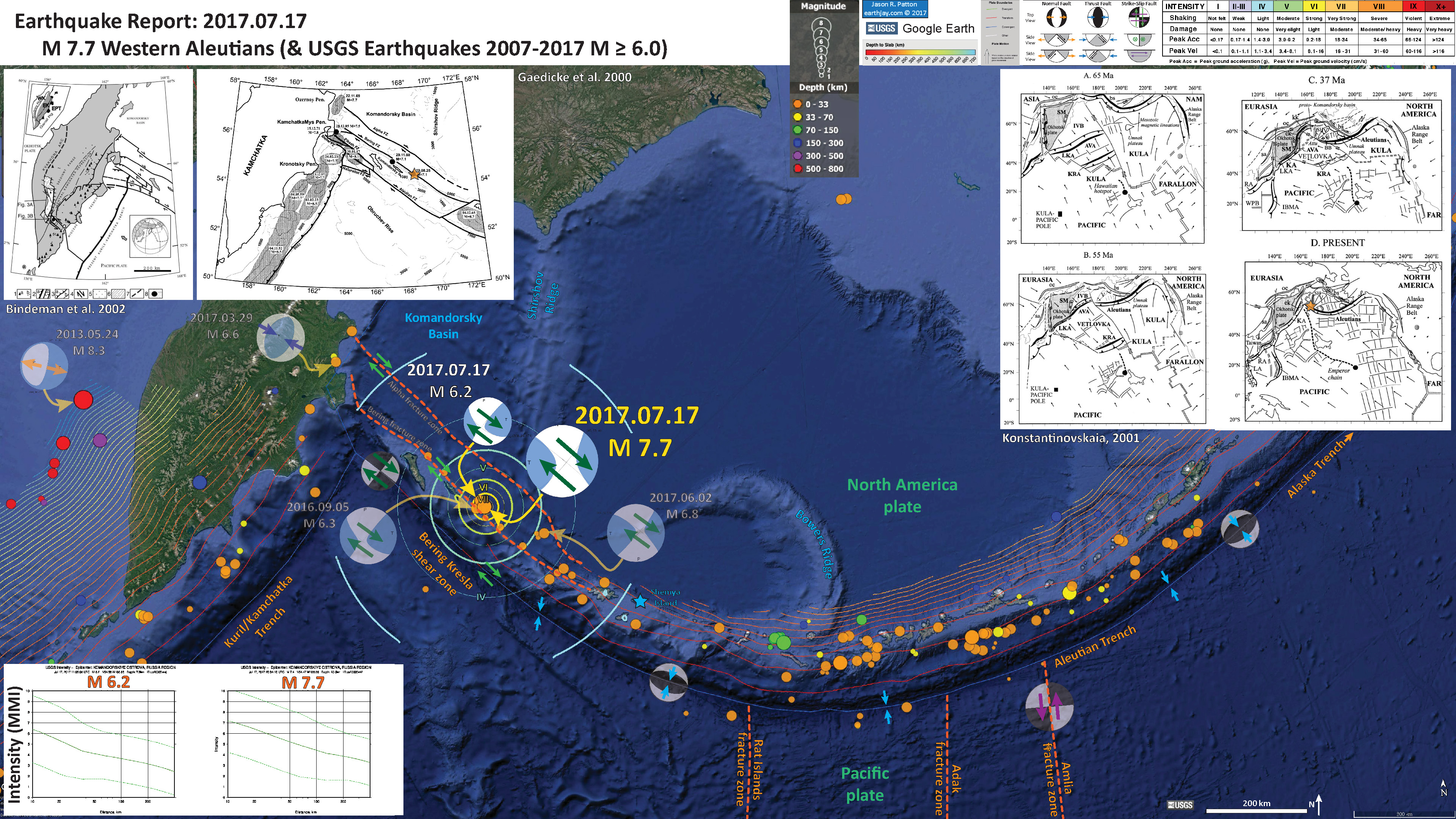
There was a similar earthquake in 2017 further to the west, which was also a strike-slip earthquake and it produced a small sized tsunami (Lay et al., 2017). However, the 17 July 2017 magnitude M 7.9 earthquake was much larger in magnitude. Here is my earthquake report and update for this 2017 earthquake. These reports include information about the intersection of the Aleutian and Kuril plate boundaries.
The majority of the Aleutian Islands are volcanic arc islands formed as a result of the subduction of the Pacific plate beneath the North America plate. To the west, there is another subduction zone along the Kuril and Kamchatka volcanic arcs. These subduction zones form deep sea trenches (the deepest parts of the ocean are in subduction zone trenches).
In the eastern part of the Aleutian/Alaska subduction zone (e.g. Alaska Peninsula or Prince William Sound), the plates converge in the direction of subduction (perpendicular to the fault orientation or “strike”). Further to the west, the plates converge obliquely compared to the fault orientation.
This oblique convergence results in the development of additional special faults that accommodate the plate convergence not perpendicular to the faults. These are typically strike-slip faults parallel to the subduction zone (they accommodate the proportion of relative motion parallel to the fault), called forearc sliver faults.
Along the central and western Aleutian plate boundary, this strike-slip relative motion also creates blocks in the upper North America plate that rotate relative to the forearc sliver fault. Imagine how ball bearings rotate when the two planes that they are contained within move relative to each other.
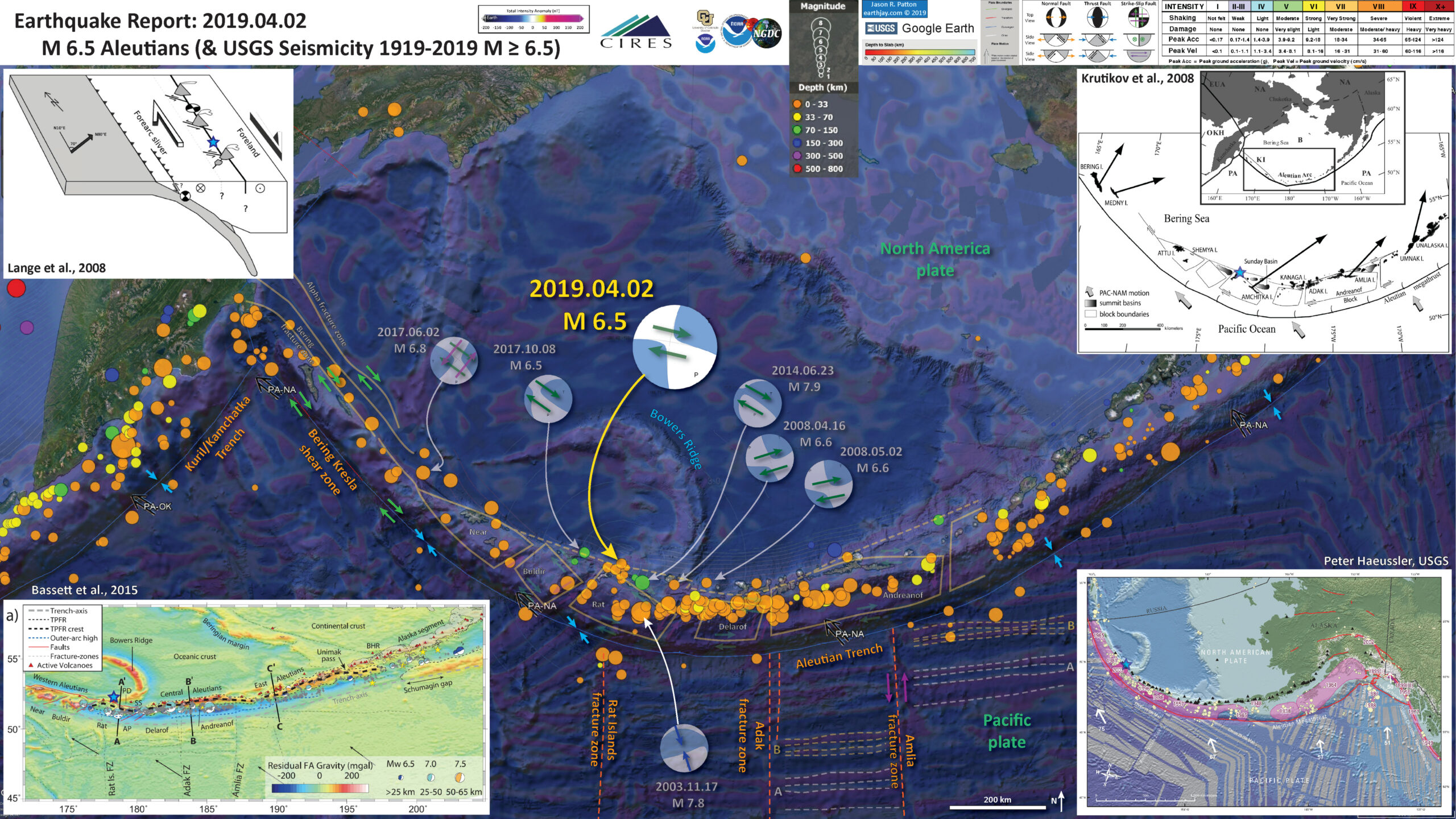
Below is my interpretive poster for this earthquake
I plot the seismicity from the past month, with color representing depth and diameter representing magnitude (see legend). I include earthquake epicenters from 1918-2018 with magnitudes M ≥ 6.5 in one version.
I plot the USGS fault plane solutions (moment tensors in blue and focal mechanisms in orange), possibly in addition to some relevant historic earthquakes.
- I placed a moment tensor / focal mechanism legend on the poster. There is more material from the USGS web sites about moment tensors and focal mechanisms (the beach ball symbols). Both moment tensors and focal mechanisms are solutions to seismologic data that reveal two possible interpretations for fault orientation and sense of motion. One must use other information, like the regional tectonics, to interpret which of the two possibilities is more likely.
- I also include the shaking intensity contours on the map. These use the Modified Mercalli Intensity Scale (MMI; see the legend on the map). This is based upon a computer model estimate of ground motions, different from the “Did You Feel It?” estimate of ground motions that is actually based on real observations. The MMI is a qualitative measure of shaking intensity. More on the MMI scale can be found here and here. This is based upon a computer model estimate of ground motions, different from the “Did You Feel It?” estimate of ground motions that is actually based on real observations.
- I include the slab 2.0 contours plotted (Hayes, 2018), which are contours that represent the depth to the subduction zone fault. These are mostly based upon seismicity. The depths of the earthquakes have considerable error and do not all occur along the subduction zone faults, so these slab contours are simply the best estimate for the location of the fault.
- In the map below, I include a transparent overlay of the magnetic anomaly data from EMAG2 (Meyer et al., 2017). As oceanic crust is formed, it inherits the magnetic field at the time. At different points through time, the magnetic polarity (north vs. south) flips, the North Pole becomes the South Pole. These changes in polarity can be seen when measuring the magnetic field above oceanic plates. This is one of the fundamental evidences for plate spreading at oceanic spreading ridges (like the Gorda rise).
- Regions with magnetic fields aligned like today’s magnetic polarity are colored red in the EMAG2 data, while reversed polarity regions are colored blue. Regions of intermediate magnetic field are colored light purple.
- We can see the roughly east-west trends of these red and blue stripes. These lines are parallel to the ocean spreading ridges from where they were formed. The stripes disappear at the subduction zone because the oceanic crust with these anomalies is diving deep beneath the North America plate \, so the magnetic anomalies from the overlying North America plate mask the evidence for the Pacific plate.
Magnetic Anomalies
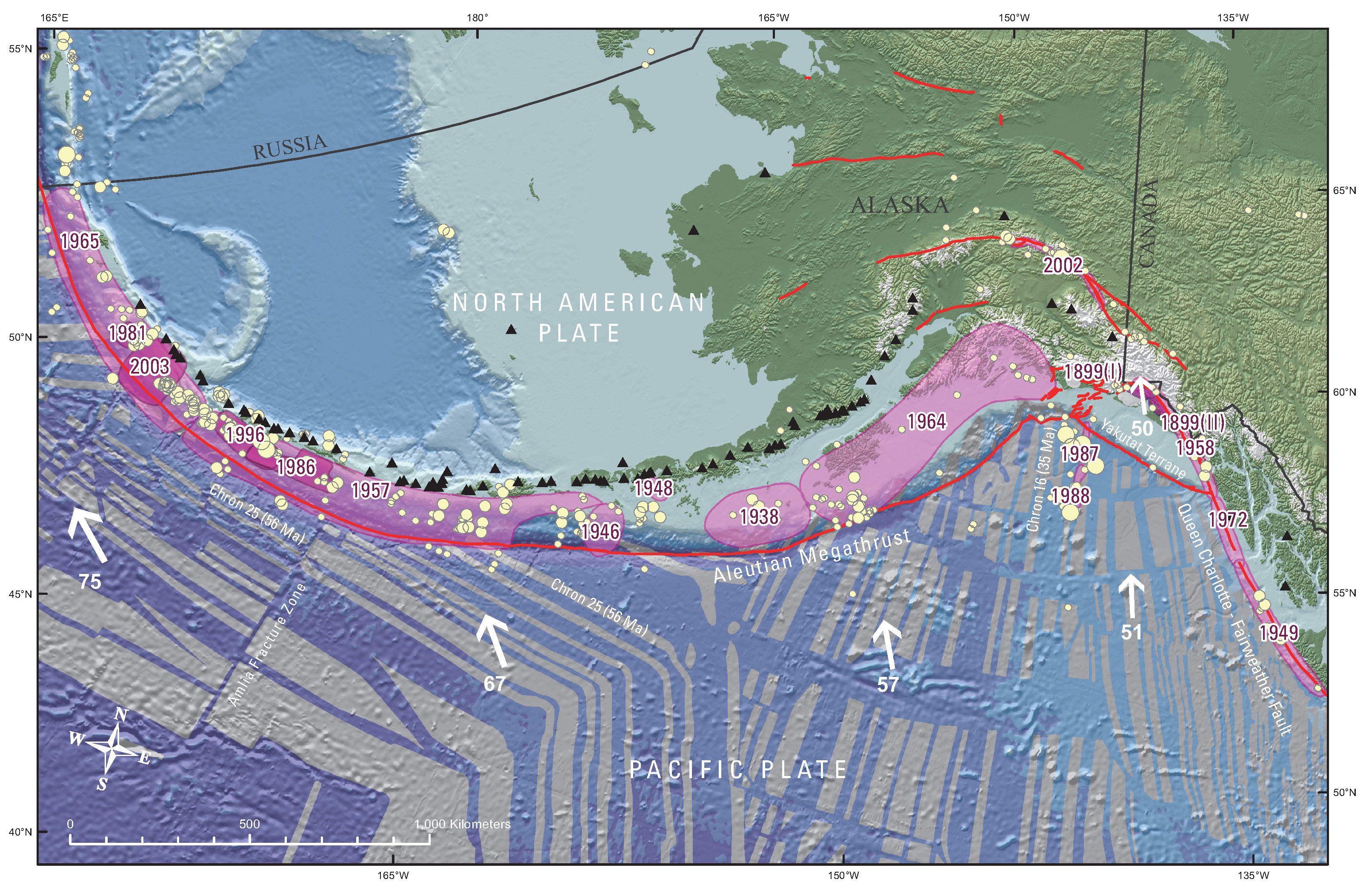
- In the lower right corner is a figure that shows the historic earthquake ruptures along the Aleutian Megathrust (Peter Haeussler, USGS). I placed a blue star in the general location of this M 6.5 quake (same for the other inset figures).
- In the upper left corner is a figure that shows how oblique relative motion between plates results in a variety of faults and fault bounded blocks (Lange et al., 2008). This example is from southern Chile (near the 1960 subduction zone earthquake).
- In the upper right corner is a plate tectonic map showing the plate boundaries (inset) and the crustal faults in the North America plate (Krutikov et al., 2008). The wide arrows show motion of Pacific plate relative to the North America plate (the direction the plate is subducting). These authors used the paleomagnetic data as evidence for rotation of fault bounded blocks.
- In the lower left corner is a figure from Bassett and Watts (2015 B) that shows the results of their analyses using gravity data.
I include some inset figures. Some of the same figures are located in different places on the larger scale map below.
- Here is the map with a month’s seismicity plotted. I outlined the blocks and labeled using Ryan and Scholl (1989) as a basemap (but very similar to Krutikov). I outlined some lineaments in the magnetic anomaly data for crust on both sides of the Amlia fracture zone and labeled these B and A (near label for Pacific plate). Note how they are offset relative to each other, demonstration of the left-lateral sense of motion here.

- Here is the map with a century’s seismicity plotted. Check out the example strike slip earthquakes, including the 2017.06.02 M 6.8 quake (that was interpreted by Lay et al., 2017 to be right lateral). Also shown is the 2003.11.17 M 7.8 subduction earthquake. Many of the other earthquakes plotted in this map are also subduction earthquakes.

- Here is the map with a century’s seismicity plotted, with megathrust earthquake patches from Peter Haeussler (USGS) outlined. I outlined the subduction zone slip patches shown in the Peter Haeussler (USGS) map. Consider how the structures in the different plates may interact with each other.

Other Report Pages
Some Relevant Discussion and Figures
- Here is a map that shows historic earthquake slip regions as pink polygons (Peter Haeussler, USGS). Dr. Haeussler also plotted the magnetic anomalies (grey regions), the arc volcanoes (black diamonds), and the plate motion vectors (mm/yr, NAP vs PP).
- Here is the figure from Sykes et al. (1980) that shows the space time relations for historic earthquakes in relation to the map.

Above: Rupture zones of earthquakes of magnitude M > 7.4 from 1925-1971 as delineated by their aftershocks along plate boundary in Aleutians, southern Alaska and offshore British Columbia [after Sykes, 1971]. Contours in fathoms. Various symbols denote individual aftershock sequences as follows: crosses, 1949, 1957 and 1964; squares, 1938, 1958 and 1965; open triangles, 1946; solid triangles, 1948; solid circles, 1929, 1972. Larger symbols denote more precise locations. C = Chirikof Island. Below: Space-time diagram showing lengths of rupture zones, magnitudes [Richter, 1958; Kanamori, 1977 b; Kondorskay and Shebalin, 1977; Kanamori and Abe, 1979; Perez and Jacob, 1980] and locations of mainshocks for known events of M > 7.4 from 1784 to 1980. Dashes denote uncertainties in size of rupture zones. Magnitudes pertain to surface wave scale, M unless otherwise indicated. M is ultra-long period magnitude of Kanamori 1977 b; Mt is tsunami magnitude of Abe[ 1979]. Large shocks 1929 and 1965 that involve normal faulting in trench and were not located along plate interface are omitted. Absence of shocks before 1898 along several portions of plate boundary reflects lack of an historic record of earthquakes for those areas.
- Here is a great illustration that shows how forearc sliver faults form due to oblique convergence at a subduction zone (Lange et al., 2008). Strain is partitioned into fault normal faults (the subduction zone) and fault parallel faults (the forearc sliver faults, which are strike-slip). This figure is for southern Chile, but is applicable globally.

Proposed tectonic model for southern Chile. Partitioning of the oblique convergence vector between the Nazca plate and South American plate results in a dextral strike-slip fault zone in the magmatic arc and a northward moving forearc sliver. Modified after Lavenu and Cembrano (1999).
- Here is a figure from Krutikov et al. (2008) that shows how blocks in the Aleutian Arc may accommodate the oblique subduction, along forearc sliver faults. Note that these blocks may also rotate to accommodate the oblique convergence. There are also margin parallel strike slip faults that bound these blocks. These faults are in the upper plate, but may impart localized strain to the lower plate, resulting in strike slip motion on the lower plate (my arm waving part of this). Note how the upper plate strike-slip faults have the same sense of motion as these deeper earthquakes.

Location map for the Aleutian Islands. The outline blocks and shaded summit basins are from Geist et al. [1988], showing a possible rotation mechanism. The heavy arrows show the mean rotations with respect to North America indicated by paleomagnetic data, the lighter arrows the motion of the Pacific plate with respect to North America. (inset) General location map modified from Chapman and Solomon [1976], Mackey et al. [1997], and Pedoja et al. [2006]. Solid lines show boundaries of plates and blocks: NA, North American Plate; B, Bering Block; PA, Pacific Plate; OKH, Okhotsk Plate; KI, Komandorsky Island Block; EUA, Eurasian Plate
- Here is a figure from Ryan and Scholl (1989) that shows their interpretation of the fault bounded blocks within the forearc shear couple.
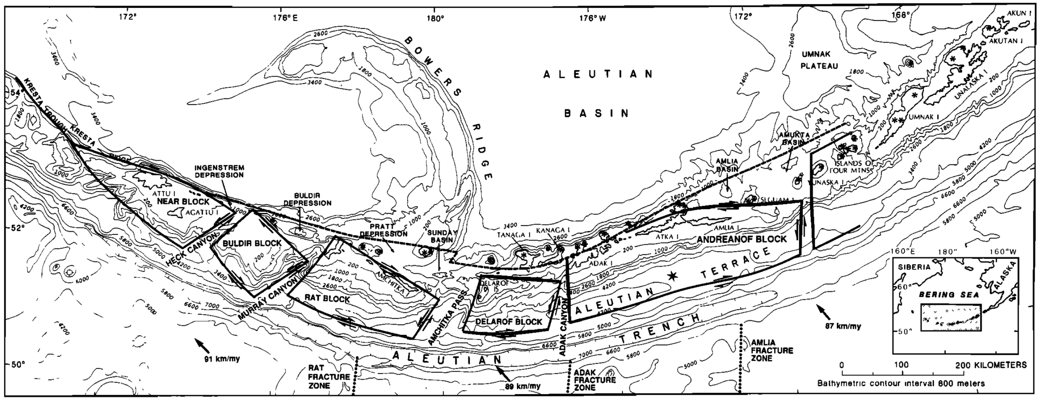
Map showing the boundaries of clockwise-rotating and westward translating blocks that comprise the Aleutian Ridge [from Geist et al. 1988]. Summit basins and transverse Pacific slope canyons are extensional structures that formed in the wake of these rotating and translating blocks. Arrows show relative plate motion between the Pacific and North American plates; convergence is increasingly oblique to the west. The central Aleutian sector lies within the Andreanof block located between Adak Canyon and Amukta Basin. A prominent summit basin has formed in the eastern part of the block (the composite Amlia and Amukta Basins). However, a summit basin is not present in the western part of the Andreanof block between Adak and Atka Islands. Asterisks show the location of active and dormant volcanoes; the star denotes the approximate location of the 1986 Andreanof earthquake.
- Here is one poster for the 17 November 2017 earthquake, from this earthquake report.
- This is a figure from Lay et al. (2017) that shows their estimate for fault slip for the 2017 temblor. This shows a northwest-southeast trending (striking) strike-slip fault. This is the slip model they used as input for their tsunami model.

(a) Bilateral slip model for the 2017 earthquake and USGS/NEIC catalog seismicity from 1900 to 16 July 2017 (blue circles, scaled proportional to magnitude, with events larger than M ~ 7 being labeled), along with all moment tensor solutions from the GCMT catalog from 1976 to 16 July 2017 (red-filled compressional quadrant focal mechanisms). (b) Foreshock seismicity on 17 July 2017 (blue circles) and aftershock seismicity in the first 2 weeks (magenta circles) along with the MW 6.3 foreshock GCMT focal mechanism (cyan focal mechanism). The large focal mechanism is the W-phase moment tensor from this study. The boxes indicate short-period radiators from the Eurasia-Greenland back projection, and stars indicate radiators from the North American back projection (Figure 3). The slip distribution is shown in detail in Figure S12. White vectors indicate the relative motion of the Pacific Plate to North America (almost identical to that relative to the Bering Plate). The large red star indicates the main shock epicenter.
- Here is a figure from Lay et al. (2017) that shows (a) their initial condition (the amount of seafloor vertical land motion that initiated the tsunami, (b) the maximum wave height map, and (c) the comparison between their model results (in red) and the observations (in black) for water surface elevations after the earthquake.

Predicted tsunami from the bilateral faulting model. (a) Final seafloor deformation with the red star indicating the epicenter and the dashed line delineating projection of the faulting model on the seafloor. (b) Predicted tsunami amplitude and DART stations (circles) considered in this study. (c) Comparison of filtered sea surface recordings (black) at DART stations with predictions (red) along with corresponding amplitude spectra (right). The recorded and predicted time series were filtered to remove signals shorter than 5 min period and the full 5 h time series were used in the computation of the amplitude spectra. The strike-slip faulting and position of the stations result in weak tsunami waves, but the timing and height of long-period arrivals provide bounds on the source.
- Here is the figure from Bassett and Watts (2015) for the Aleutians.

Aleutian subduction zone. Symbols as in Figure 3. (a) Residual free-air gravity anomaly and seismicity. The outer-arc high, trench-parallel fore-arc ridge and block-bounding faults are dashed in blue, black, and red, respectively. Annotations are AP = Amchitka Pass; BHR = Black-Hills Ridge; SS = Sunday Sumit Basin; PD = Pratt Depression. (b) Published asperities and slip-distributions/aftershock areas for large magnitude earthquakes. (c) Cross sections showing residual bathymetry (green), residual free-air gravity anomaly (black), and the geometry of the seismogenic zone [Hayes et al., 2012].
- Here is the schematic figure from Bassett and Watts (2015).

Schematic diagram summarizing the key spatial associations interpreted between the morphology of the fore-arc and variations in the seismogenic behavior of subduction megathrusts.
- Here are several figures from Konstantnovskaia et al. (2001) showing their tectonic reconstructions. I include their figure captions below in blockquote. The first figure is the one included in the poster above.
- Here are 4 panels that show the details of their reconstructions. Panels shown are for 65 Ma, 55 Ma, 37 Ma, and Present.

Geodynamic setting of Kamchatka in framework of the Northwest Pacific. Modified after Nokleberg et al. (1994) and Kharakhinov (1996)). Simplified cross-section line I-I’ is shown in Fig. 2. The inset shows location of Sredinny and Eastern Ranges. [More figure caption text in the publication].


The Cenozoic evolution in the Northwest Pacific. Plate kinematics is shown in hotspot reference frame after (Engebretson et al., 1985). Keys distinguish zones of active volcanism (thick black lines), inactive volcanic belts (thick gray lines), deformed arc terranes (hatched pattern), subduction zones: active (black triangles), inactive *(empty triangles). In letters: sa = Sikhote-aline, bs = Bering shelf belts; SH = Shirshov Ridge; V = Vitus arch; KA = Kuril; RA = Ryukyu’ LA = Luzon; IBMA = Izu-Bonin-Mariana arcs; WPB = Western Philippine, BB = Bowers basins.
- Here is a beautiful illustration for the Aleutian Trench from Alpha (1973) as posted on the David Rumsey Collection online.

Geologic Fundamentals
- For more on the graphical representation of moment tensors and focal mechanisms, check this IRIS video out:
- Here is a fantastic infographic from Frisch et al. (2011). This figure shows some examples of earthquakes in different plate tectonic settings, and what their fault plane solutions are. There is a cross section showing these focal mechanisms for a thrust or reverse earthquake. The upper right corner includes my favorite figure of all time. This shows the first motion (up or down) for each of the four quadrants. This figure also shows how the amplitude of the seismic waves are greatest (generally) in the middle of the quadrant and decrease to zero at the nodal planes (the boundary of each quadrant).

- Here is another way to look at these beach balls.
The two beach balls show the stike-slip fault motions for the M6.4 (left) and M6.0 (right) earthquakes. Helena Buurman's primer on reading those symbols is here. pic.twitter.com/aWrrb8I9tj
— AK Earthquake Center (@AKearthquake) August 15, 2018
- There are three types of earthquakes, strike-slip, compressional (reverse or thrust, depending upon the dip of the fault), and extensional (normal). Here is are some animations of these three types of earthquake faults. The following three animations are from IRIS.
Strike Slip:
Compressional:
Extensional:
- This is an image from the USGS that shows how, when an oceanic plate moves over a hotspot, the volcanoes formed over the hotspot form a series of volcanoes that increase in age in the direction of plate motion. The presumption is that the hotspot is stable and stays in one location. Torsvik et al. (2017) use various methods to evaluate why this is a false presumption for the Hawaii Hotspot.
- Here is a map from Torsvik et al. (2017) that shows the age of volcanic rocks at different locations along the Hawaii-Emperor Seamount Chain.
- Here is a great tweet that discusses the different parts of a seismogram and how the internal structures of the Earth help control seismic waves as they propagate in the Earth.

A cutaway view along the Hawaiian island chain showing the inferred mantle plume that has fed the Hawaiian hot spot on the overriding Pacific Plate. The geologic ages of the oldest volcano on each island (Ma = millions of years ago) are progressively older to the northwest, consistent with the hot spot model for the origin of the Hawaiian Ridge-Emperor Seamount Chain. (Modified from image of Joel E. Robinson, USGS, in “This Dynamic Planet” map of Simkin and others, 2006.)

Hawaiian-Emperor Chain. White dots are the locations of radiometrically dated seamounts, atolls and islands, based on compilations of Doubrovine et al. and O’Connor et al. Features encircled with larger white circles are discussed in the text and Fig. 2. Marine gravity anomaly map is from Sandwell and Smith.
Today, on #SeismogramSaturday: what are all those strangely-named seismic phases described in seismograms from distant earthquakes? And what do they tell us about Earth’s interior? pic.twitter.com/VJ9pXJFdCy
— Jackie Caplan-Auerbach (@geophysichick) February 23, 2019
- Summary of the 1964 Earthquake
- 2019.03.26 M 5.2 Alaska
- 2019.04.02 M 6.5 Aleutians
- 2018.12.20 M 7.4 Bering Kresla
- 2018.12.20 M 7.3 Bering Kresla UPDATE #1
- 2018.11.30 M 7.0 Alaska
- 2018.08.15 M 6.6 Aleutians
- 2018.08.12 M 6.4 North Alaska
- 2018.08.12 M 6.4 North Alaska UPDATE #1
- 2018.01.23 M 7.9 Gulf of Alaska
- 2018.01.23 M 7.9 Gulf of Alaska UPDATE #1
- 2018.01.23 M 7.9 Gulf of Alaska UPDATE #2
- 2017.07.17 M 7.7 Aleutians
- 2017.07.17 M 7.7 Aleutians UPDATE #1
- 2017.06.02 M 6.8 Aleutians
- 2017.05.08 M 6.2 Aleutians
- 2017.05.01 M 6.3 British Columbia
- 2017.03.29 M 6.6 Kamchatka
- 2017.03.02 M 5.5 Alaska
- 2016.09.05 M 6.3 Bering Kresla (west of Aleutians)
- 2016.04.13 M 5.7 & 6.4 Kamchatka
- 2016.04.02 M 6.2 Alaska Peninsula
- 2016.03.27 M 5.7 Aleutians
- 2016.03.12 M 6.3 Aleutians
- 2016.01.29 M 7.2 Kamchatka
- 2016.01.24 M 7.1 Alaska
- 2015.11.09 M 6.2 Aleutians
- 2015.11.02 M 5.9 Aleutians
- 2015.11.02 M 5.9 Aleutians (update)
- 2015.07.27 M 6.9 Aleutians
- 2015.05.29 M 6.7 Alaska Peninsula
- 2015.05.29 M 6.7 Alaska Peninsula (animations)
- 1964.03.27 M 9.2 Good Friday
Alaska | Kamchatka | Kurile
General Overview
Earthquake Reports
Social Media
- Abe, K., 1972. Lithospheric Normal Faulting Beneath the Aleutian Trench in Phys. Earth Planet. Interiors, v. 5, p. 1990-198.
- Bassett and Watts, 2015 A. Gravity anomalies, crustal structure, and seismicity at subduction zones: 1. Seafloor roughness and subducting relief in Geochemistry, Geophysics, Geosystems, v. 16, doi:10.1002/2014GC005684.
- Bassett, D. and Watts, A.B., 2015 B. Gravity anomalies, crustal structure, and seismicity at subduction zones: 2. Interrelationships between fore-arc structure and seismogenic behavior in Geochemistry, Geophysics, Geosystems, v. 16, doi:10.1002/2014GC005685.
- Brown, J.R., Prejan, S.G., Beroza, G.C., Gomberg, J.S., and Hauessler,m P.J., 2013. Deep low-frequency earthquakes in tectonic tremor along the Alaska-Aleutian subduction zone in JGR Solid Earth, v. 118, p. 1079-1090, doi:10.1029/2012JB009459
- Ikuta, R., Mitsui, Y., Kurokawa, Y., and Ando, M., 2015. Evaluation of strain accumulation in global subduction zones from seismicity data in Earth, Planets and Space, v. 67, DOI 10.1186/s40623-015-0361-5
- Frisch, W., Meschede, M., Blakey, R., 2011. Plate Tectonics, Springer-Verlag, London, 213 pp.
- Gaedicke, C., Baranov, B., Seliverstov, N., Alexeiev, D., Tsukanov, N., Freitag, R., 2000. Structure of an active arc-continent collision area: the Aleutian-Kamchatka junction. Tectonophysics 325, 63–85
- Hayes, G. P., D. J. Wald, and R. L. Johnson, 2012. Slab1.0: A three-dimensional model of global subduction zone geometries, J. Geophys. Res., 117, B01302, doi:10.1029/2011JB008524.
- Hayes, G., 2018, Slab2 – A Comprehensive Subduction Zone Geometry Model: U.S. Geological Survey data release, https://doi.org/10.5066/F7PV6JNV.
- Koulakov, I.Y., Dobretsov, N.L., Bushenkova, N.A., and Yakovlev, A.V., 2011. Slab shape in subduction zones beneath the Kurile–Kamchatka and Aleutian arcs based on regional tomography results in Russian Geology and Geophysics, v. 52, p. 650-667.
- Konstantnovskaia, 2001. Arc-continent collision and subduction reversal in the Cenozoic evolution of the Northwest Pacific: an example from Kamchatka (NE Russia) in Tectonophysics, v. 333, p. 75-94.
- Krutikov, L., Stone, D.B., and Minyuk, P., 2008. New Paleomagnetic Data From the Central Aleutian Arc: Evidence and Implications for Block Rotations in Active Tectonics and Seismic Potential of Alaska, Geophysical Monograph Series 179 American Geophysical Union. 10.1029/179GM07
- Lange, D., Cembrano, J., Rietbrock, A., Haberland, C., Dahm, T., and Bataille, K., 2008. First seismic record for intra-arc strike-slip tectonics along the Liquiñe-Ofqui fault zone at the obliquely convergent plate margin of the southern Andes in Tectonophysics, v. 455, p. 14-24
- Lay, T., H. Kanamori, C. J. Ammon, A. R. Hutko, K. Furlong, and L. Rivera, 2009. The 2006 – 2007 Kuril Islands great earthquake sequence in J. Geophys. Res., 114, B11308, doi:10.1029/2008JB006280.
- Lay, T., Ye, L., Bai, Y., Cheung, K. F., Kanamori, H., Freymueller, J., … Kogan, M. G. (2017). Rupture along 400 km of the Bering fracture zone in the Komandorsky Islands earthquake (MW 7.8) of 17 July 2017. Geophysical Research Letters, 44, 12,161–12,169. https://doi.org/10.1002/2017GL076148
- Meyer, B., Saltus, R., Chulliat, a., 2017. EMAG2: Earth Magnetic Anomaly Grid (2-arc-minute resolution) Version 3. National Centers for Environmental Information, NOAA. Model. https://doi.org/10.7289/V5H70CVX
- Müller, R.D., Sdrolias, M., Gaina, C. and Roest, W.R., 2008, Age spreading rates and spreading asymmetry of the world’s ocean crust in Geochemistry, Geophysics, Geosystems, 9, Q04006, https://doi.org/10.1029/2007GC001743
- Plafker, G., 1972. Alaskan earthquake of 1964 and Chilean earthquake of 1960: Implications for arc tectonics in Journal of Geophysical Research, v. 77, p. 901-925.
- Portnyagin, M. and Manea, V.C., 2008. Mantle temperature control on composition of arc magmas along the Central Kamchatka Depression in Geology, v. 36, no. 7, p. 519-522.
- Rhea, S., Tarr, A.C., Hayes, G., Villaseñor, A., Furlong, K.P., and Benz, H.M., 2010. Seismicity of the Earth 1900-2007, Kuril-Kamchatka arc and vicinity: U.S. Geological Survey Open-File Report 2010-1083-C, 1 map sheet, scale 1:5,000,000.
- Saltus, R.W., and Barnett, A., 2000. Eastern Aleutian Volcanic Arc Digital Model – Version 1.0: U.S. Geological Survey Open-File Report 00
- Stauyder, W., 1968. Mechanism of the Rat Island Earthquake Sequence of February 4, 1965, with Relation to Island Arcs and Sea-Floor Spreading in JGR, v. 73, no. 12, p. 3847-3858
- Sykes, L.R., Kissinger, J.B>, House, L., Davies, J.N>, and Jacob, K.H., 1980. Rupture Zones and Repeat Times of Great Earthquakes Along the Alaska-Aleutian Arc, 1784-1980, in Maurice Ewing Series, Earthquake Prediction, An International Review, AGU
- Torsvik, T. H. et al., 2017. Pacific plate motion change caused the Hawaiian-Emperor Bend in Nat. Commun., v. 8, doi: 10.1038/ncomms15660
- Wilson, J. Tuzo, 1963. “A possible origin of the Hawaiian Islands” in Canadian Journal of Physics. v. 41, p. 863–870 doi:10.1139/p63-094.
References:
Return to the Earthquake Reports page.