Gibbons and others (2015) have put together a suite of geologic data (e.g. ages of geologic units, fossils), plate motion data (geometry of plates and ocean ridge spreading rates), and plate tectonic data (initiation and cessation of subduction or collision, obduction of ophiolites) to create a global plate tectonic map that spans the past 200 million years (Ma). Here is the facebook post that I first saw to include this video.
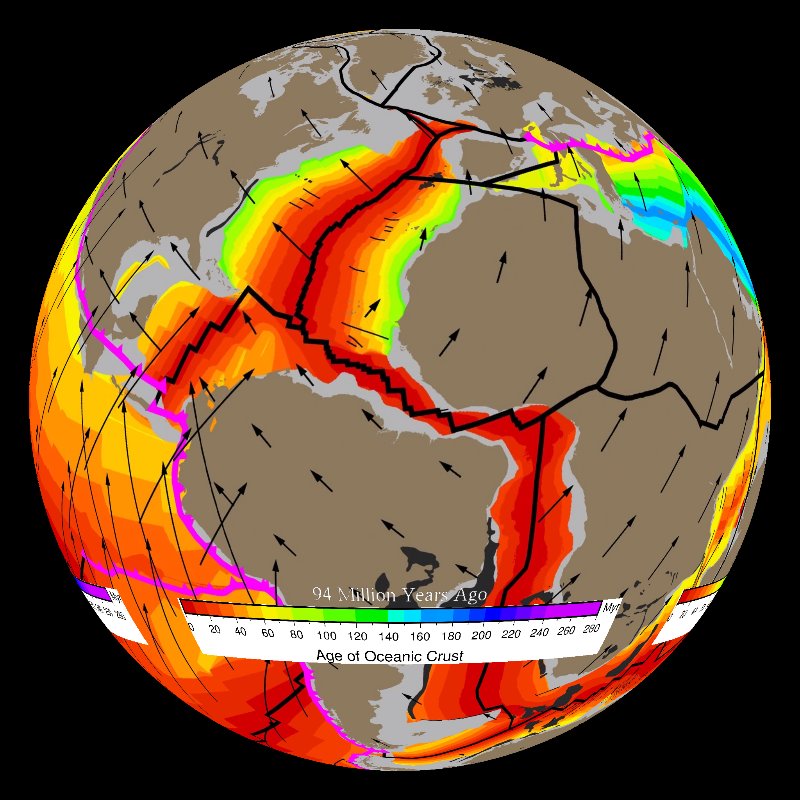
Here is a view of their tectonic map at a specific time.

Gibbons et al. (2015) created several animations using their plate tectonic model. I have embedded both of these videos below. Other versions of these files are placed on the NOAA Science on a Sphere Program website.
- This is a direct link to the embedded video below.
Here is the first animation.
- This is a direct link to the embedded video below.
Here is the second animation.
They also compare their model with P-wave tomographic analytical results. P-Wave tomography works similar to CT-scans. CT-scans are the the result of integrating X-Ray data, from many 3-D orientations, to model the 3-D spatial variations in density. “CT” is an acronym for “computed tomography.” Both are kinds of tomography. Here is a book about seismic tomography. Here is a paper from Goes et al. (2002) that discusses their model of the thermal structure of the uppermost mantle in North America as inferred from seismic tomography.
Here is an illustration from the wiki page that that attempts to help us visualize what tomography is.

P-Wave tomography uses Seismic P-Waves to model the 3-D spatial variation of Earth’s internal structure. P-Wave tomography is similar to Computed-Tomography of X-Rays because the P-wave sources are also in different spatial locations. For CT-scans, the variation in density is inferred with the model. For P-Wave tomography, the variation in seismic velocity. Typically, when seismic waves travel faster, they are travelling through old, cold, and more dense crust/lithosphere/mantle. Likewise, when seismic waves travel slower, they are travelling through relatively young, hot, and less dense crust/lithosphere/mantle.
Regions of Earth’s interior that have faster seismic velocities are often plotted in blue. Regions that have slower velocities are often plotted in red.
Here are their plots showing the velocity perturbation (faster or slower). I include the figure caption below the image.


Plate reconstructions superimposed on age-coded depth slices from P-wave seismic tomography (Li et al., 2008) using first-order assumptions of near-vertical slab sinking, with a) 3.0 and 1.2 cm/yr constant sinking rates in the upper and lower mantle, respectively, following Zahirovic et al. (2012), and b) 5.0 and 2.0 cm/yr upper and lower mantle sinking rates, respectively, following Replumaz et al. (2004). Both end-member sinking rates indicate bands of slab material (blue, S1–S2) offset southward from the Andean-style subduction zone along southern Lhasa, consistentwith the interpretations of Tethyan subducted slabs by Hafkenscheid et al. (2006). However, although the P-wave tomography provides higher resolution than S-wave tomography, the amplitude of the velocity perturbation is significantly lower in oceanic regions (e.g., S2) and the southern hemisphere due to continental sampling biases. Orthographic projection centered on 0°N, 90°E.
-
References:
- Gibbons, A., Zahirovic, S., Muller, R., Whittaker, J., and Yatheesh, V., 2015. A tectonic model reconciling evidence for the collisions between India, Eurasia and intra-oceanic arcs of the central-eastern Tethys in Gondwana Research, v. 28, p. 451-492.
- Goes, S. and van der Lee, S.. 2002. Thermal structure of the North American uppermost mantle inferred from seismic tomography in Journal of Geophysical Research, v. 107, no. B3, 2050, DOI. 10.1029/2000JB000049
- Hafkenscheid, E., Wortel, M., Spakman, W., 2006. Subduction history of the Tethyan region derived from seismic tomography and tectonic reconstructions in Journal of Geophysical Research – Solid Earth 111, B08401.
- Replumaz, A., Kárason, H., van der Hilst, R.D., Besse, J., Tapponnier, P., 2004. 4-D evolution of SE Asia’s mantle from geological reconstructions and seismic tomography in Earth and Planetary Science Letters 221, 103–115.
- Zahirovic, S., Müller, R.D., Seton, M., Flament, N., Gurnis, M., Whittaker, J., 2012. Insights on the kinematics of the India–Eurasia collision from global geodynamic models in Geochemistry, Geophysics, Geosystems 13.