Earthquake Report: 1700 Cascadia subduction zone 317 year commemoration

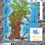
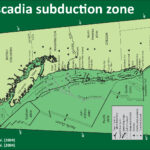
Today (possibly tonight at about 9 PM) is the birthday of the last known Cascadia subduction zone (CSZ) earthquake. There is some evidence that there have been more recent CSZ earthquakes (e.g. late 19th century in southern OR / northern CA), but they were not near full margin ruptures (where the entire fault, or most of it, slipped during the earthquake).
I have been posting material about the CSZ for the past couple of years here and below are some prior Anniversary posts, as well as Earthquake Reports sorted according to their region along the CSZ. Below I present some of the material included in those prior reports (to help bring it all together), but I have prepared a new map for today’s report as well.


On this evening, 317 years ago, the Cascadia subduction zone fault ruptured as a margin wide earthquake. I here commemorate this birthday with some figures that are in two USGS open source professional papers. The Atwater et al. (2005) paper discusses how we came to the conclusion that this last full margin earthquake happened on January 26, 1700 at about 9 PM (there may have been other large magnitude earthquakes in Cascadia in the 19th century). The Goldfinger et al. (2012) paper discusses how we have concluded that the records from terrestrial paleoseismology are correlable and how we think that the margin may have ruptured in the past (rupture patch sizes and timing). The reference list is extensive and this is but a tiny snapshot of what we have learned about Cascadia subduction zone earthquakes. Brian Atwater and his colleagues have updated the Orphan Tsunami and produced a second edition available here for download and here for hard copy purchase (I have a hard copy).

Here is a map of the Cascadia subduction zone, modified from Nelson et al. (2006). The Juan de Fuca and Gorda plates subduct northeastwardly beneath the North America plate at rates ranging from 29- to 45-mm/yr. Sites where evidence of past earthquakes (paleoseismology) are denoted by white dots. Where there is also evidence for past CSZ tsunami, there are black dots. These paleoseismology sites are labeled (e.g. Humboldt Bay). Some submarine paleoseismology core sites are also shown as grey dots. The two main spreading ridges are not labeled, but the northern one is the Juan de Fuca ridge (where oceanic crust is formed for the Juan de Fuca plate) and the southern one is the Gorda rise (where the oceanic crust is formed for the Gorda plate).


Today I prepared this new map showing the results of shakemap scenario model prepared by the USGS. I prepared this map using data that can be downloaded from the USGS website here. Shakemaps show what we think might happen during an earthquake, specifically showing how strongly the ground might shake. There are different measures of this, which include Peak Ground Acceleration (PGA), Peak Ground Velocity (PGV), and Modified Mercalli Intensity (MMI). More background information about the shakemap program at the USGS can be found here. One thing that all of these measures share is that they show that there is a diminishing of ground shaking with distance from the earthquake. This means that the further from the earthquake, the less strongly the shaking will be felt. This can be seen on the maps below. The USGS prepares shakemaps for all earthquakes with sufficiently large magnitudes (i.e. we don’t need shakemaps for earthquakes of magnitude M = 1.5). An archive of these USGS shakemaps can be found here. All the scenario USGS shakemaps can be found here.
I chose to use the MMI representation of ground shaking because it is most easily comparable for people to understand. This is because MMI scale is designed based upon relations between ground shaking intensity and observations that people are able to make (e.g. how strongly they felt the earthquake, how much objects in their residences or places of business responded, how much buildings were damaged, etc.).
The MMI ground motion model is based upon a computer model estimate of ground motions, different from the “Did You Feel It?” estimate of ground motions that is actually based on real observations. More on the MMI scale can be found here and here.


Here is the USGS version of this map. The outline of the fault that was used to generate the ground motions that these maps are based upon is outlined in black.


I prepared an end of the year summary for earthquakes along the CSZ. Below is my map from this Earthquake Report.

  • Here is the map where I show the epicenters as circles with colors designating the age. I also plot the USGS moment tensors for each earthquake, with arrows showing the sense of motion for each earthquake.
  • I placed a moment tensor / focal mechanism legend in the lower left corner of the map. There is more material from the USGS web sites about moment tensors and focal mechanisms (the beach ball symbols). Both moment tensors and focal mechanisms are solutions to seismologic data that reveal two possible interpretations for fault orientation and sense of motion. One must use other information, like the regional tectonics, to interpret which of the two possibilities is more likely.
  • In some cases, I am able to interpret the sense of motion for strike-slip earthquakes. In other cases, I do not know enough to be able to make this interpretation (so I plot both solutions).

    I include some inset figures in the poster.

  • In the upper left corner is a map of the Cascadia subduction zone (CSZ) and regional tectonic plate boundary faults. This is modified from several sources (Chaytor et al., 2004; Nelson et al., 2004)
  • Below the CSZ map is an illustration modified from Plafker (1972). This figure shows how a subduction zone deforms between (interseismic) and during (coseismic) earthquakes. Today’s earthquake did not occur along the CSZ, so did not produce crustal deformation like this. However, it is useful to know this when studying the CSZ.
  • To the lower right of the Cascadia map and cross section is a map showing the latest version of the Uniform California Earthquake Rupture Forecast (UCERF). Let it be known that this is not really a forecast, and this name was poorly chosen. People cannot forecast earthquakes. However, it is still useful. The faults are colored vs. their likelihood of rupturing. More can be found about UCERF here. Note that the San Andreas fault, and her two sister faults (Maacama and Bartlett Springs), are orange-red.
  • To the upper right of the Cascadia map and cross section is a map showing the shaking intensities based upon the USGS Shakemap model. Earthquake Scenarios describe the expected ground motions and effects of specific hypothetical large earthquakes. The color scale is the same as found on many of my #EarthquakeReport interpretive posters, the Modified Mercalli Intensity Scale (MMI). The latest version of this map is here.
  • In the upper right corner I include generalized fault map of northern California from Wallace (1990).
  • To the left of the Wallace (1990) map is a figure that shows the evolution of the San Andreas fault system since 30 million years ago (Ma). This is a figure from the USGS here.
  • In the lower right corner I include the Earthquake Shaking Potential map from the state of California. This is a probabilistic seismic hazard map, basically a map that shows the likelihood that there will be shaking of a given amount over a period of time. More can be found from the California Geological Survey here. I place a yellow star in the approximate location of today’s earthquake.


This figure shows how a subduction zone deforms between (interseismic) and during (coseismic) earthquakes. We also can see how a subduction zone generates a tsunami. Atwater et al., 2005.


Here is a version of the CSZ cross section alone (Plafker, 1972).


Here is an animation produced by the folks at Cal Tech following the 2004 Sumatra-Andaman subduction zone earthquake. I have several posts about that earthquake here and here. One may learn more about this animation, as well as download this animation here.

Here is a graphic showing the sediment-stratigraphic evidence of earthquakes in Cascadia. Atwater et al., 2005. There are 3 panels on the left, showing times of (1) prior to earthquake, (2) several years following the earthquake, and (3) centuries after the earthquake. Before the earthquake, the ground is sufficiently above sea level that trees can grow without fear of being inundated with salt water. During the earthquake, the ground subsides (lowers) so that the area is now inundated during high tides. The salt water kills the trees and other plants. Tidal sediment (like mud) starts to be deposited above the pre-earthquake ground surface. This sediment has organisms within it that reflect the tidal environment. Eventually, the sediment builds up and the crust deforms interseismically until the ground surface is again above sea level. Now plants that can survive in this environment start growing again. There are stumps and tree snags that were rooted in the pre-earthquake soil that can be used to estimate the age of the earthquake using radiocarbon age determinations. The tree snags form “ghost forests.


Here is a photo of the ghost forest, created from coseismic subsidence during the Jan. 26, 1700 Cascadia subduction zone earthquake. Atwater et al., 2005.


Here is a photo I took in Alaska, where there was a subduction zone earthquake in 1964. These tree snags were living trees prior to the earthquake and remain to remind us of the earthquake hazards along subduction zones.


This shows how a tsunami deposit may be preserved in the sediment stratigraphy following a subduction zone earthquake, like in Cascadia. Atwater et al., 2005. If there is a source of sediment to be transported by a tsunami, it will come along for the ride and possibly be deposited upon the pre-earthquake ground surface. Following the earthquake, tidal sediment is deposited above the tsunami transported sediment. Sometimes plants that were growing prior to the earthquake get entombed within the tsunami deposit.


The NOAA/NWS/Pacific Tsunami Warning Center has updated their animation of the simulation of the 1700 “Orphan Tsunami.”
Source: Nathan C. Becker, Ph.D. nathan.becker at noaa.gov

Below are some links and embedded videos.

  • Here is the yt link for the embedded video below.
  • Here is the mp4 link for the embedded video below. (2160p 145 mb mp4)
  • Here is the mp4 link for the embedded video below. (1080p 145 mb mp4)

  • Here is the text associated with this animation:

    Just before midnight on January 27, 1700 a tsunami struck the coasts of Japan without warning since no one in Japan felt the earthquake that must have caused it. Nearly 300 years later scientists and historians in Japan and the United States solved the mystery of what caused this “orphan tsunami” through careful analysis of historical records in Japan as well as oral histories of Native Americans, sediment deposits, and ghost forests of drowned trees in the Pacific Northwest of North America, a region also known as Cascadia. They learned that this geologically active region, the Cascadia Subduction Zone, not only hosts erupting volcanoes but also produces megathrust earthquakes capable of generating devastating, ocean-crossing tsunamis. By comparing the tree rings of dead trees with those still living they could tell when the last of these great earthquakes struck the region. The trees all died in the winter of 1699-1700 when the coasts of northern California, Oregon, and Washington suddenly dropped 1-2 m (3-6 ft.), flooding them with seawater. That much motion over such a large area requires a very large earthquake to explain it—perhaps as large as 9.2 magnitude, comparable to the Great Alaska Earthquake of 1964. Such an earthquake would have ruptured the earth along the entire length of the 1000 km (600 mi) -long fault of the Cascadia Subduction Zone and severe shaking could have lasted for 5 minutes or longer. Its tsunami would cross the Pacific Ocean and reach Japan in about 9 hours, so the earthquake must have occurred around 9 o’clock at night in Cascadia on January 26, 1700 (05:00 January 27 UTC).

    The Pacific Tsunami Warning Center (PTWC) can create an animation of a historical tsunami like this one using the same too that they use for determining tsunami hazard in real time for any tsunami today: the Real-Time Forecasting of Tsunamis (RIFT) forecast model. The RIFT model takes earthquake information as input and calculates how the waves move through the world’s oceans, predicting their speed, wavelength, and amplitude. This animation shows these values through the simulated motion of the waves and as they race around the globe one can also see the distance between successive wave crests (wavelength) as well as their height (half-amplitude) indicated by their color. More importantly, the model also shows what happens when these tsunami waves strike land, the very information that PTWC needs to issue tsunami hazard guidance for impacted coastlines. From the beginning the animation shows all coastlines covered by colored points. These are initially a blue color like the undisturbed ocean to indicate normal sea level, but as the tsunami waves reach them they will change color to represent the height of the waves coming ashore, and often these values are higher than they were in the deeper waters offshore. The color scheme is based on PTWC’s warning criteria, with blue-to-green representing no hazard (less than 30 cm or ~1 ft.), yellow-to-orange indicating low hazard with a stay-off-the-beach recommendation (30 to 100 cm or ~1 to 3 ft.), light red-to-bright red indicating significant hazard requiring evacuation (1 to 3 m or ~3 to 10 ft.), and dark red indicating a severe hazard possibly requiring a second-tier evacuation (greater than 3 m or ~10 ft.).

    Toward the end of this simulated 24-hours of activity the wave animation will transition to the “energy map” of a mathematical surface representing the maximum rise in sea-level on the open ocean caused by the tsunami, a pattern that indicates that the kinetic energy of the tsunami was not distributed evenly across the oceans but instead forms a highly directional “beam” such that the tsunami was far more severe in the middle of the “beam” of energy than on its sides. This pattern also generally correlates to the coastal impacts; note how those coastlines directly in the “beam” have a much higher impact than those to either side of it.

    Offshore, Goldfinger and others (from the 1960’s into the 21st Century, see references in Goldfinger et al., 2012) collected cores in the deep sea. These cores contain submarine landslide deposits (called turbidites). These turbidites are thought to have been deposited as a result of strong ground shaking from large magnitude earthquakes. Goldfinger et al. (2012) compile their research in the USGS professional paper. This map shows where the cores are located.


    Here is an example of how these “seismoturbidites” have been correlated. The correlations are the basis for the interpretation that these submarine landslides were triggered by Cascadia subduction zone earthquakes. This correlation figure demonstrates how well these turbidites have been correlated. Goldfinger et al., 2012.


    This map shows the various possible prehistoric earthquake rupture regions (patches) for the past 10,000 years. Goldfinger et al., 2012. These rupture scenarios have been adopted by the USGS hazards team that determines the seismic hazards for the USA.


    Here is an update of this plot given new correlations from recent work (Goldfinger et al., 2016).


    Here is a plot showing the earthquakes in a linear timescale.


    I combined the plot above into another figure that includes all the recurrence intervals and segment lengths in a single figure. This is modified from Goldfinger et al. (2012).

    http://earthquake.usgs.gov/earthquakes/shakemap/global/shake/casc9.0_expanded_peak_se/

Earthquake Report: 2016 Summary Cascadia

Here I summarize the seismicity for Cascadia in 2016. I limit this summary to earthquakes with magnitude greater than or equal to M 4.0. I reported on all but five of these earthquakes. I put this together a couple weeks ago, but wanted to wait to post until the new year (just in case that there was another earthquake to include).
I prepared a 2016 annual summary for Earth here.

    I include summaries of my earthquake reports in sorted into three categories. One may also search for earthquakes that may not have made it into these summary pages (use the search tool).

  • Magnitude
  • Region
  • Year

Earthquake Summary Poster (2016)

  • Here is the map where I show the epicenters as circles with colors designating the age. I also plot the USGS moment tensors for each earthquake, with arrows showing the sense of motion for each earthquake.
  • I placed a moment tensor / focal mechanism legend in the lower left corner of the map. There is more material from the USGS web sites about moment tensors and focal mechanisms (the beach ball symbols). Both moment tensors and focal mechanisms are solutions to seismologic data that reveal two possible interpretations for fault orientation and sense of motion. One must use other information, like the regional tectonics, to interpret which of the two possibilities is more likely.
  • In some cases, I am able to interpret the sense of motion for strike-slip earthquakes. In other cases, I do not know enough to be able to make this interpretation (so I plot both solutions).

    I include some inset figures in the poster.

  • In the upper left corner is a map of the Cascadia subduction zone (CSZ) and regional tectonic plate boundary faults. This is modified from several sources (Chaytor et al., 2004; Nelson et al., 2004)
  • Below the CSZ map is an illustration modified from Plafker (1972). This figure shows how a subduction zone deforms between (interseismic) and during (coseismic) earthquakes. Today’s earthquake did not occur along the CSZ, so did not produce crustal deformation like this. However, it is useful to know this when studying the CSZ.
  • To the lower right of the Cascadia map and cross section is a map showing the latest version of the Uniform California Earthquake Rupture Forecast (UCERF). Let it be known that this is not really a forecast, and this name was poorly chosen. People cannot forecast earthquakes. However, it is still useful. The faults are colored vs. their likelihood of rupturing. More can be found about UCERF here. Note that the San Andreas fault, and her two sister faults (Maacama and Bartlett Springs), are orange-red.
  • To the upper right of the Cascadia map and cross section is a map showing the shaking intensities based upon the USGS Shakemap model. Earthquake Scenarios describe the expected ground motions and effects of specific hypothetical large earthquakes. The color scale is the same as found on many of my #EarthquakeReport interpretive posters, the Modified Mercalli Intensity Scale (MMI). The latest version of this map is here.
  • In the upper right corner I include generalized fault map of northern California from Wallace (1990).
  • To the left of the Wallace (1990) map is a figure that shows the evolution of the San Andreas fault system since 30 million years ago (Ma). This is a figure from the USGS here.
  • In the lower right corner I include the Earthquake Shaking Potential map from the state of California. This is a probabilistic seismic hazard map, basically a map that shows the likelihood that there will be shaking of a given amount over a period of time. More can be found from the California Geological Survey here. I place a yellow star in the approximate location of today’s earthquake.


    Cascadia subduction zone: General Overview

  • Cascadia’s 315th Anniversary 2015.01.26
  • Cascadia’s 316th Anniversary 2016.01.26
  • Earthquake Information about the CSZ 2015.10.08

The big player this year was an M 6.5 along the Mendocino fault on 2016.12.08. Here I present an inventory of 8 earthquakes with M ≥ 5.0. There are a few additional earthquakes with smaller magnitudes that are of particular interest.

Please visit the #EarthquakeReport pages for more information about the figures that I include in the Earthquake Report interpretive posters below.


    References

  • Atwater, B.F., Musumi-Rokkaku, S., Satake, K., Tsuju, Y., Eueda, K., and Yamaguchi, D.K., 2005. The Orphan Tsunami of 1700—Japanese Clues to a Parent Earthquake in North America, USGS Professional Paper 1707, USGS, Reston, VA, 144 pp.
  • Chaytor, J.D., Goldfinger, C., Dziak, R.P., and Fox, C.G., 2004. Active deformation of the Gorda plate: Constraining deformation models with new geophysical data: Geology v. 32, p. 353-356.
  • Dengler, L.A., Moley, K.M., McPherson, R.C., Pasyanos, M., Dewey, J.W., and Murray, M., 1995. The September 1, 1994 Mendocino Fault Earthquake, California Geology, Marc/April 1995, p. 43-53.
  • Geist, E.L. and Andrews D.J., 2000. Slip rates on San Francisco Bay area faults from anelastic deformation of the continental lithosphere, Journal of Geophysical Research, v. 105, no. B11, p. 25,543-25,552.
  • Irwin, W.P., 1990. Quaternary deformation, in Wallace, R.E. (ed.), 1990, The San Andreas Fault system, California: U.S. Geological Survey Professional Paper 1515, online at: http://pubs.usgs.gov/pp/1990/1515/
  • McLaughlin, R.J., Sarna-Wojcicki, A.M., Wagner, D.L., Fleck, R.J., Langenheim, V.E., Jachens, R.C., Clahan, K., and Allen, J.R., 2012. Evolution of the Rodgers Creek–Maacama right-lateral fault system and associated basins east of the northward-migrating Mendocino Triple Junction, northern California in Geosphere, v. 8, no. 2., p. 342-373.
  • Nelson, A.R., Asquith, A.C., and Grant, W.C., 2004. Great Earthquakes and Tsunamis of the Past 2000 Years at the Salmon River Estuary, Central Oregon Coast, USA: Bulletin of the Seismological Society of America, Vol. 94, No. 4, pp. 1276–1292
  • Rollins, J.C. and Stein, R.S., 2010. Coulomb stress interactions among M ≥ 5.9 earthquakes in the Gorda deformation zone and on the Mendocino Fault Zone, Cascadia subduction zone, and northern San Andreas Fault: Journal of Geophysical Research, v. 115, B12306, doi:10.1029/2009JB007117, 2010.
  • Stoffer, P.W., 2006, Where’s the San Andreas Fault? A guidebook to tracing the fault on public lands in the San Francisco Bay region: U.S. Geological Survey General Interest Publication 16, 123 p., online at http://pubs.usgs.gov/gip/2006/16/
  • Wallace, Robert E., ed., 1990, The San Andreas fault system, California: U.S. Geological Survey Professional Paper 1515, 283 p. [http://pubs.usgs.gov/pp/1988/1434/].

Toast, tsunamis, and the really big one | Chris Goldfinger | TEDxMtHood

Following an article in the New Yorker on July 20, 2015, the Cascadia subduction zone got more attention nationwide than it had ever seen previously. Most in the pacific northwest knew about Cascadia, but this article brought knowledge of the hazards to a national audience. A follow up article on July 28, 2015, the author Kathryn Shultz, wrote about how people can prepare for a CSZ earthquake and tsunami. Shultz was awarded a Pulitzer Prize for Feature Writing and a National Magazine Award for “The Really Big One,” recognition for her writing and the impact of this article.
On May 18, 2016, Dr. Chris Goldfinger presented a TEDx talk for TEDxMtHood. His talk was about the Cascadia subduction zone. This is a great talk for lay persons (most people). Here is Dr. Goldfinger’s OSU website. Here is Dr. Goldfinger’s earthquake blog.

    I provide more background information on the CSZ in several places.

  • Cascadia’s 315th Anniversary 2015.01.26
  • Earthquake Information about the CSZ 2015.10.08
  • Cascadia Paleoearthquakes 2012/03/11
    Here is what Dr. Goldfinger wrote to introduce his talk online.

  • I wondered why a crowd of New Yorkers would be interested in earthquakes. Several hundred gathered last October to hear a panel discuss “The Really Big One,” a New Yorker article about the Pacific Northwest that went viral after revealing to many what we geologists have known for a long time.
  • We were the warm-up acts for the “real stars” of the New Yorker Festival: Billy Joel, Norman Lear and the like… So I asked the crowd to imagine that someone came on the evening news one day and reported the discovery of a new, very large fault, a subduction zone that ran from Virginia to Newfoundland, generating magnitude 9 earthquakes on a regular basis, and would soon destroy New York.
  • Well, that exact scenario is not going to happen, but it did happen in the Northwest. It wasn’t a sudden thing, the news of this has been dribbling out over 30 years, so when the New Yorker article came out, I expected nothing to happen really.
  • But, instead, the story went viral and revealed something startling and new to the country, and even to a lot of Northwesterners – all of whom I was pretty sure had heard this information before. After all, it had been the subject of numerous documentaries, and tons of print and television news stories. And really, to west coast-centric me, the New Yorker was just a magazine with not-very-funny cartoons that piled up in dentists’ offices.
  • But what the article revealed was not not-new information, but rather that the story was not well known at all.
  • My inbox filled up with hundreds of emails from people all around the region, wondering if they would be “toast” living west of I-5, wondering if a tsunami would come up the Columbia to destroy Portland, and even wondering if one would come over the coast range and “get” Medford. Really, I’m not making this up. Not that we’re not in a tough spot: we are. But what is the reality?
  • The geologic records of previous earthquakes now stretches back ~ 10,000 years making Cascadia as we call it, the best-known fault on Earth. We can’t know when the next earthquake will come.
  • I think we’re collectively still blinking and hoping we heard something wrong. But the evidence is now about as airtight as it gets, so what to do? We have an opportunity to prepare for this and save lives. Will we learn from others and from the past and do it right?
  • This is what I’m going to talk about at TEDxMtHood this June: the seriousness of The Big One, and how we can all be prepared when it hits.
  • Here is a low angle oblique cross section of the CSZ.

    Here is a short bio for Dr. Goldfinger.

  • Dr. Chris Goldfinger is a marine geologist and geophysicist whose focus is on great earthquakes and the structure of subduction zones around the world. He is experienced using deep submersibles, multi-beam and side scan sonar, seismic reflection, and other marine geophysical tools all over the world. Recently, Chris was in the national spotlight after being featured in Kathryn Schulz’s article in The New Yorker, “The Really Big One.” His extensive research on the Cascadia subduction zone yielded an earthquake record extending through the Holocene epoch helping to develop a model of segmentation and earthquake recurrence. Conclusion: our area is overdue for a major earthquake.
  • Originally hailing from Palo Alto, Chris married a Salem girl and is currently Professor of Marine Geology at Oregon State University. His dad worked for NASA; so growing up in a house filled with stuff from the early probes like Voyager, Ranger, Surveyor, etc. made interest in earth sciences a natural progression. He is also into windsurfing, ocean sailing, and aerobatic flying.

Earthquake mini-swarm near La Pine, OR!

Over the past day or so, there has been a swarm of seismicity in the La Pine area. La Pine is on the east side of the Cascade mountain range, a magmatic arc related to the Cascadia subduction zone. As the downgoing Juan de Fuca plate extends into the upper mantle, the sea water stored in the oceanic crust (which formed under water) combines with the increased heat to melt. This melt is less dense than the crust and surrounding mantle material, so it rises. This rising magma gives rise to the volcanoes in the Cascade range. There exist every type of volcano in the Cascades due to the wide range of magma composition along the arc.
Today’s largest magnitude earthquake has a magnitude M = 3.0. This is too small to get a moment tensor or focal mechanism calculated, so we do not know what type of earthquake this is. However, we can surmise that it is either compressional or extensional, probably not shear (strike-slip). The swarm may be related to back arc extension, or may be related to some magmatic processes. I favor the former since these earthquakes plot between a series of mapped Quaternary active faults. To the west is Hamner Butte and the the north is Davis Mountain. To the north, there does appear to be some north-northeast lineaments that suggest some fault related volcanism. To the south there also are mapped faults called the Chemult graben fault system (see Personius references below). These are normal faults, so the likely mechanism for earthquakes in this swarm is extensional. The last activity on these faults predate the Mazama ash since they are overlain by a pyroclastic flow from that eruption. The latest age estimate for the eruption of Mt. Mazama is based on Bayesian modeling of many radiocarbon age determinations by Egan et al. (2015) and set at 7682–7584 cal. yr BP (95.4% probability range). However, Pezzopane (1993) classify this fault system as late Pleistocene.
Here is the USGS web page for this M = 3.0 earthquake. In addition to the compilation from Personius (see below), work has been done on the faulting in this region by Pezzopane (1993) and Pezzopane and Weldon (1993). Weldon et al. (2003) map most of the faults in this region as late Quaternary (<780 ka) in age. This is a map that shows the locality for this mini swarm.

This is a map that shows the region, that extends across the Cascades.


This is a map of the Cascdia subduction zone and Cascade magmatic arc.


Here is a view of the subduction zone showing the landscape and the plate configuration within the Earth. The cross section is located near the southern Willamette Valley. This is schematic and does not completely match the real geography. Note how the downgoing plate melts and the rising magma leads to volcanism of the Cascade volcanoes (a volcanic arc).


Dr. John Vidale, from the Pacific Northwest Seismic Network posted this today showing the seismic record of these earthquakes.


Dr. Vidale also plotted the cumulative number of earthquakes in this region for the past 12 years.


This area is at the western boundary of the High Lava Plains, where they meet the Cascades. Newberry Crater, which is where the 2000 Pacific Northwest Cell Friends of the Pleistocene field trip met, is to the northeast of this swarm. Here is a map that shows the volcanism of the region from Meigs et al. (2009). Below is the caption from Meigs et al. (2009).

Volcanic and tectonic elements of the western United States: (A) Distribution of volcanic rocks younger than 17 Ma, by age and composition (Luedke and Smith, 1984), illustrates the tremendous volcanic activity east of the Cascade Range in the northern extent of the Basin and Range province. (B) Some tectonic elements (after Jordan et al., 2004) superimposed on the map of Luedke and Smith (1984). Solid brown line outlines the Basin and Range province. Volcanic fields younger than 5 Ma illustrate the continuing activity in the Cascade Range and along the High Lava Plains (HLP; brown field) and the eastern Snake River Plain (ESRP). Short curves along the HLP and ESRP are isochrons (ages in Ma) for the migrating silicic volcanism along each volcanic trace. Flood basalt activity was fed from dike systems in the northern Nevada rift (NNR), Steens Mountain (SM), the western Snake River Plain (WSRP) and the Chief Joseph (CJ) and Cornucopia (C) dike swarms of the Columbia River Basalt Group. These dikes occur near the western border of Precambrian North America as defined by the 87Sr/86Sr 0.706 line (large dot-dash line). Northwest-trending fault systems—Olympic-Wallowa lineament (OWL), Vale (V), Brothers (B), Eugene-Denio (ED) and McLoughlin (Mc)—are shown by the short-dashed lines. Additional features include Newberry Volcano (NB), Owyhee Plateau (OP), Juan de Fuca Plate, San Andreas fault zone (SAFZ), and Mendocino triple junction (MTJ).CA—California; ID—Idaho; OR—Oregon; NV—Nevada; UT— Utah; WA—Washington; WY—Wyoming.

Here is the Weldon et al. (2002) map of faults in this region.

    References:

  • Chaytor, J.D., Goldfinger, C., Dziak, R.P., and Fox, C.G., 2004. Active deformation of the Gorda plate: Constraining deformation models with new geophysical data in Geology, v. 32, p. 353-356
  • Egan, J., Staff, R., and Blackford, J., 2015. A high-precision age estimate of the Holocene Plinian eruption of Mount Mazama, Oregon, USA in The Holocene
  • Meigs, A., Scarberry, K., Grunder, A., Carlson, R., Ford, M.T., Fouch, M., Grove, T., Hart, W.K., Iademarco, M., Jordan, B., Milliard, J., Streck, M.J., Trench, D., and Weldon, R., 2009. Geological and geophysical perspectives on the magmatic and tectonic development, High Lava Plains and northwest Basin and Range, in O’Connor, J.E., Dorsey, R.J., and Madin, I.P., eds., Volcanoes to Vineyards: Geologic Field Trips through the Dynamic Landscape of the Pacific Northwest: Geological Society of America Field Guide 15, p. 435–470, doi: 10.1130/2009.fl d015(21).
  • Nelson, A.R., Kelsey, H.M., Witter, R.C., 2006. Great earthquakes of variable magnitude at the Cascadia subduction zone in Quaternary Research 65, 354-365.
  • Personius, S.F., compiler, 2002. Fault number 839a, Chemult graben fault system, western section, in Quaternary fault and fold database of the United States: U.S. Geological Survey website, http://earthquakes.usgs.gov/hazards/qfaults, accessed 10/22/2015 10:08 PM.
  • Personius, S.F., compiler, 2002. Fault number 839b, Chemult graben fault system, Walker Rim section, in Quaternary fault and fold database of the United States: U.S. Geological Survey website, http://earthquakes.usgs.gov/hazards/qfaults, accessed 10/22/2015 10:09 PM.
  • Pezzopane, S.K., 1993, Active faults and earthquake ground motions in Oregon: Eugene, Oregon, University of Oregon, unpublished Ph.D. dissertation, 208 p.
  • Pezzopane, S.K. and Weldon, R.J.III., 1993. Tectonic Role of Active Faulting in Central Oregon in Tectonics, v. 12, no. 5, p. 1140-1169.
  • Weldon, R.J., Fletcher, D.K., Weldon, E.M., Scharer, K.M., and McCrory, P.A., 2003. An update of Quaternary faults of central and eastern Oregon: U.S. Geological Survey Open-File Report 02-301 (CD-ROM), 26 sheets, scale 1:100,000

Cascadia subduction zone: Tectonic Earthquakes of the Pacific Northwest

IRIS and the US Geological Survey have recently produced an educational video about tectonic earthquakes in the region of the US Pacific Northwest. The project was funded by the National Science Foundation.

The Video

YT link for the embedded video below.
mp4 link for the embedded video below.
mp4 embedded video:


YT embedded video:

I recently collected a core with a thick sandy deposit that is hypothesized to be the sedimentary deposit that was the result of tsunami deposition following the 1700 A.D. Cascadia subduction zone earthquake. Here is my post about that core.
Here is a composite of the two cores that I collected. The top of the core is on the left. Some interpret this to be the 1700 AD tsunami deposit.

  • YT link for the embedded video below:

Earlier this year was the 315th anniversary of the 1700 AD Cascadia subduction zone earthquake and tsunami. I compiled some information about that earthquake and tsunami. I included some information about the plate tectonics of the region. Here is the post for that anniversary.
Here is a map of the Cascadia subduction zone, modified from Nelson et al. (2006). The Juan de Fuca and Gorda plates subduct norteastwardly beneath the North America plate at rates ranging from 29- to 45-mm/yr. Sites where evidence of past earthquakes (paleoseismology) are denoted by white dots. Where there is also evidence for past CSZ tsunami, there are black dots. These paleoseismology sites are labeled (e.g. Humboldt Bay). Some submarine paleoseismology core sites are also shown as grey dots. The two main spreading ridges are not labeled, but the northern one is the Juan de Fuca ridge (where oceanic crust is formed for the Juan de Fuca plate) and the southern one is the Gorda rise (where the oceanic crust is formed for the Gorda plate).


This map (McCrory et al., 2006) shows the secular (ongoing modern) rates of motion for the Juan de Fuca and Gorda plates relative to the North America plate (Wilson, 1998; McCrory, 2000). Red triangles denote active arc volcanoes.


Here is a view of the subduction zone showing the landscape and the plate configuration within the Earth. The cross section is located near the southern Willamette Valley. This is schematic and does not completely match the real geography. Note how the downgoing plate melts and the rising magma leads to volcanism of the Cascade volcanoes (a volcanic arc).


Here is a version of the CSZ cross section alone (Plafker, 1972).


This figure shows how a subduction zone deforms between (interseismic) and during (coseismic) earthquakes. We also can see how a subduction zone generates a tsunami. Atwater et al., 2005.


Here is an animation produced by the folks at Cal Tech following the 2004 Sumatra-Andaman subduction zone earthquake. I have several posts about that earthquake here and here. One may learn more about this animation, as well as download this animation here.

This figure shows the regions that participate in this interseismic and coseismic deformation at Cascadia. Atwater et al., 2005. Black dots on the map show sites where evidence for coseismic subsidence has been found in coastal marshes, lakes, and estuaries.


This shows how the CSZ is deforming vertically today (Wang et al., 2003). The panel on the right shows the vertical motion in mm/yr.


This figure, also from Wang et al. (2003), shows their estimate of how the coseismic vertical motion may happen. Contours are in meters.


Here is a graphic showing the sediment-stratigraphic evidence of earthquakes in Cascadia. Atwater et al., 2005. There are 3 panels on the left, showing times of (1) prior to earthquake, (2) several years following the earthquake, and (3) centuries after the earthquake. Before the earthquake, the ground is sufficiently above sea level that trees can grow without fear of being inundated with salt water. During the earthquake, the ground subsides (lowers) so that the area is now inundated during high tides. The salt water kills the trees and other plants. Tidal sediment (like mud) starts to be deposited above the pre-earthquake ground surface. This sediment has organisms within it that reflect the tidal environment. Eventually, the sediment builds up and the crust deforms interseismically until the ground surface is again above sea level. Now plants that can survive in this environment start growing again. There are stumps and tree snags that were rooted in the pre-earthquake soil that can be used to estimate the age of the earthquake using radiocarbon age determinations. The tree snags form “ghost forests.


Here is a photo of the ghost forest, created from coseismic subsidence during the Jan. 26, 1700 Cascadia subduction zone earthquake. Atwater et al., 2005.


Here is a photo I took in Alaska, where there was a subduction zone earthquake in 1964. These tree snags were living trees prior to the earthquake and remain to remind us of the earthquake hazards along subduction zones.


This shows how a tsunami deposit may be preserved in the sediment stratigraphy following a subduction zone earthquake, like in Cascadia. Atwater et al., 2005. If there is a source of sediment to be transported by a tsunami, it will come along for the ride and possibly be deposited upon the pre-earthquake ground surface. Following the earthquake, tidal sediment is deposited above the tsunami transported sediment. Sometimes plants that were growing prior to the earthquake get entombed within the tsunami deposit.


Here is a new animation of the tsunami that was triggered during the 1700 AD CSZ earthquake. This is just a model and has considerable uncertainty associated with it. From the US NWS Pacific Tsunami Warning Center (PTWC).

This is the timeline of prehistoric earthquakes as preserved in sediment stratigraphy in Grays Harbor and Willapa Bay, Washington. Atwater et al., 2005. This timeline is based upon numerous radiocarbon age determinations for materials that died close to the time of the prehistoric earthquakes inferred from the sediment stratigraphy at locations along the Grays Harbor, Willapa Bay, and Columbia River estuary paleoseismic sites.


Offshore, Goldfinger and others (from the 1960’s into the 21st Century, see references in Goldfinger et al., 2012) collected cores in the deep sea. These cores contain submarine landslide deposits (called turbidites). These turbidites are thought to have been deposited as a result of strong ground shaking from large magnitude earthquakes. Goldfinger et al. (2012) compile their research in the USGS professional paper. This map shows where the cores are located.


Here is an example of how these “seismoturbidites” have been correlated. The correlations are the basis for the interpretation that these submarine landslides were triggered by Cascadia subduction zone earthquakes. This correlation figure demonstrates how well these turbidites have been correlated. Goldfinger et al., 2012


This map shows the various possible prehistoric earthquake rupture regions (patches) for the past 10,000 years. Goldfinger et al., 2012. These rupture scenarios have been adopted by the USGS hazards team that determines the seismic hazards for the USA.


I have a paper that also discusses the paleoseismology and sedimentary settings in Cascadia (and Sumatra). Patton et al., 2013.
Here is my abstract:

Turbidite deposition along slope and trench settings is evaluated for the Cascadia and Sumatra–Andaman subduction zones. Source proximity, basin effects, turbidity current flow path, temporal and spatial earthquake rupture, hydrodynamics, and topography all likely play roles in the deposition of the turbidites as evidenced by the vertical structure of the final deposits. Channel systems tend to promote low-frequency components of the content of the current over longer distances, while more proximal slope basins and base-of-slope apron fan settings result in a turbidite structure that is likely influenced by local physiography and other factors. Cascadia’s margin is dominated by glacial cycle constructed pathways which promote turbidity current flows for large distances. Sumatra margin pathways do not inherit these antecedent sedimentary systems, so turbidity currents are more localized.

The Gorda plate is deforming due to north-south compression between the Pacific and Juan de Fuca plates. There have been many papers written about this. The most recent and comprehensive review is from Jason Chaytor (Chaytor et al., 2004). Here is a map of the Cascadia subduction zone, as modified from Nelson et al. (2006) and Chaytor et al. (2004). I have updated the figure to be good for projections in a dark room (green) and to have the correct sense of motion on the two transform plate boundaries at either end of the CSZ (Queen Charlotte and San Andreas faults).


Here is the Chaytor et al. (2004) map that shows their interpretation of the structural relations in the Gorda plate.


Here is a map from Rollins and Stein, showing their interpretations of different historic earthquakes in the region. This was published in response to the Januray 2010 Gorda plate earthquake. The faults are from Chaytor et al. (2004).


The Blanco fracture zone is also an active transform plate boundary. The BFZ is a strike slip fault system that connects two spreading ridges, the Gorda Rise and the Juan de Fuca Ridge. Here is a map that shows the tectonic setting and some earthquakes related to the BFZ from April 2015. There are some animations on this web page showing seismicity with time along the BFZ, over the past 15
years.

References:

Plate Tectonics: 200 Ma

Gibbons and others (2015) have put together a suite of geologic data (e.g. ages of geologic units, fossils), plate motion data (geometry of plates and ocean ridge spreading rates), and plate tectonic data (initiation and cessation of subduction or collision, obduction of ophiolites) to create a global plate tectonic map that spans the past 200 million years (Ma). Here is the facebook post that I first saw to include this video.
Here is a view of their tectonic map at a specific time.


Gibbons et al. (2015) created several animations using their plate tectonic model. I have embedded both of these videos below. Other versions of these files are placed on the NOAA Science on a Sphere Program website.

They also compare their model with P-wave tomographic analytical results. P-Wave tomography works similar to CT-scans. CT-scans are the the result of integrating X-Ray data, from many 3-D orientations, to model the 3-D spatial variations in density. “CT” is an acronym for “computed tomography.” Both are kinds of tomography. Here is a book about seismic tomography. Here is a paper from Goes et al. (2002) that discusses their model of the thermal structure of the uppermost mantle in North America as inferred from seismic tomography.
Here is an illustration from the wiki page that that attempts to help us visualize what tomography is.


P-Wave tomography uses Seismic P-Waves to model the 3-D spatial variation of Earth’s internal structure. P-Wave tomography is similar to Computed-Tomography of X-Rays because the P-wave sources are also in different spatial locations. For CT-scans, the variation in density is inferred with the model. For P-Wave tomography, the variation in seismic velocity. Typically, when seismic waves travel faster, they are travelling through old, cold, and more dense crust/lithosphere/mantle. Likewise, when seismic waves travel slower, they are travelling through relatively young, hot, and less dense crust/lithosphere/mantle.
Regions of Earth’s interior that have faster seismic velocities are often plotted in blue. Regions that have slower velocities are often plotted in red.
Here are their plots showing the velocity perturbation (faster or slower). I include the figure caption below the image.


Plate reconstructions superimposed on age-coded depth slices from P-wave seismic tomography (Li et al., 2008) using first-order assumptions of near-vertical slab sinking, with a) 3.0 and 1.2 cm/yr constant sinking rates in the upper and lower mantle, respectively, following Zahirovic et al. (2012), and b) 5.0 and 2.0 cm/yr upper and lower mantle sinking rates, respectively, following Replumaz et al. (2004). Both end-member sinking rates indicate bands of slab material (blue, S1–S2) offset southward from the Andean-style subduction zone along southern Lhasa, consistentwith the interpretations of Tethyan subducted slabs by Hafkenscheid et al. (2006). However, although the P-wave tomography provides higher resolution than S-wave tomography, the amplitude of the velocity perturbation is significantly lower in oceanic regions (e.g., S2) and the southern hemisphere due to continental sampling biases. Orthographic projection centered on 0°N, 90°E.

Springfield Earthquake!

It took me a couple days to catch up with things, so I missed posting about this earthquake until now.
We had a Mw = 4.2 earthquake northeast of Eugene on the morning of 2015.07.04. Here is the USGS web page for this earthquake. The hypocentral depth is 9.9 km, well above the Cascadia subduction zone fault (which is at approximately 52 km depth in this location, based upon McCrory et al., 2012).
Here is a map that shows the faulting in and around the Willamette River Valley. Eugene and Springfield are in the southern portion of the map and Salem is in the northernmost portion of the map. I rubbersheeted (georeferenced) this map from the Bob Yeats text, Living with Earthquakes in the Pacific Northwest (Yeats, 2004). The entire text from Yeat’s book is online and available as a pdf. There is a Quaternary fault (active in at least the last 2.5 million years) called the Upper Willamette River fault (UWRF) that strikes northwest and aligns sub-parallel to hwy 58 (the orange line in the southeast/lower-right part of the map). The epicenter is plotted as an orange dot. I placed the moment tensor for this earthquake, along with a legend showing how to interpret the moment tensor. There are blue arrows showing a northeast-southwest oriented maximum stress orientation (compression in the direction of the blue arrows). The UWRF points directly at the epicenter, so it may be that the UWRF extends further to the northwest.


This is the “Did You Feel It?” map that uses the Modified Mercalli Intensity Scale to display the relative ground shaking across the region. This earthquake was broadly felt. These data are based upon the results from observations made by people as reported to the USGS on this web page.


This plot shows how the ground motions attenuate with distance from the earthquake. The green line (and orange line, which is difficult to see) is based upon empirical models of ground shaking based upon seismologic records from thousands of earthquakes in California. The blue dots are observations from real people and the orange dots are the median observed intensities for different distance bins (with bars that show the uncertainty to +-1 standard deviation). The take away is that the further away from the epicenter, the lower the ground motions. Secondly, that the empirical relations fit the data pretty well, but not perfectly. Note the large variation in ground motions at any given Hypocentral Distance (in km).


Here is a figure from McCaffrey et al. (2007) that shows how the North America plate is possibly chopped up into blocks. Each “block” has a structural affinity to itself (positions within each block move together in a similar direction/orientation that are statistically different than the motions of positions on adjacent blocks). The upper map shows the motions of these positions as they move related to “stable” North America. Each arrow is a vector that show the direction and magnitude of the rate of movement (mm/yr) at that position. The middle panel shows the relative northward motion of these positions at latitudes of 40, 42.5, and 45 degrees north (transects are shown in color on the upper panel/map). The steps in the rates show the boundaries of the blocks as modeled by McCaffrey et al. (2007). The lowest panel shows a schematic of these blocks as they relate to each other. I am not yet sure how the UWRF fits into this block model, but it is a part of the tectonics in this region.

Blanco Fracture Zone: 2000 – 2015 Seismicity Animation

I put together an animation that includes the seismicity from 1/1/2000 until 6/1/2015 for the region near the Blanco fracture zone, with earthquake magnitudes greater than or equal to M = 5.0. The map here shows all these epicenters, with the moment tensors for earthquakes of M = 6 or more (plus the two largest earthquakes from today’s swarm). This is the search that I used for the earthquakes plotted in the map and animations below. Here is the page that I posted regarding the beginning of this swarm. Here is a post from some earthquakes last year along the BFZ.
Earthquake epicenters are plotted with the depth designated by color and the magnitude depicted by the size of the circle. These are all fairly shallow earthquakes at depths suitable for oceanic lithosphere.

    Here is the list of the earthquakes with moment tensors plotted in the above maps (with links to the USGS websites for those earthquakes):

  • 2000/06/02 M 6.0
  • 2003/01/16 M 6.3
  • 2008/01/10 M 6.3
  • 2012/04/12 M 6.0
  • 2015/06/01 M 5.8
  • 2015/06/01 M 5.9
    Here are some files that are outputs from that USGS search above.

  • csv file
  • kml file (not animated)
  • kml file (animated)

VIDEOS

    Here are links to the video files (it might be easier to download them and view them remotely as the files are large).

  • First Animation (20 mb mp4 file)
  • Second Animation (10 mb mp4 file)

Here is the first animation that first adds the epicenters through time (beginning with the oldest earthquakes), then removes them through time (beginning with the oldest earthquakes).


Here is the second animation that uses a one-year moving window. This way, one year after an earthquake is plotted, it is removed from the plot. This animation is good to see the spatiotemporal variation of seismicity along the BFZ.

Here is a map with all the fore- and after-shocks plotted to date.


Late addition:
Here is a seismogram from Gold Mountain Washington. Thanks for posting this Pacific Northwest Seismic Network fb page. Here is the page that it came from.

Blanco fracture zone strikes again

The Blanco fracture zone (BFZ) is a transform plate boundary that connects the Juan de Fuca ridge with the Gorda rise spreading centers. This active fault zone consists of numerous right-lateral (dextral) faults. There is some debate as to how far east the BFZ extends beyond the Gorda rise (some pose it extends far past the trench and ambient noise tomographic data supports this interpretation; Porritt et al., 2011). I remember a colleague of mine who once adamantly stated that there is no evidence for the extension of the BFZ eastwards past the megathrust fault tip. However, they were working on faulting in the North America plate along coastal Oregon, so their view was limited (compared to the plot I share below). However, this colleague made this statement a decade before the Porritt et al. (2011) data were to be published.
There were two Mw 4.2 earthquakes associated with this plate boundary fault system in the past week. I plot the moment tensors for these earthquakes (USGS pages: 4/7/15 and 4/11/15) in this map below. I also have placed the relative plate motions as arrows, labeled the plates, and placed a transparent focal mechanism plot above the BFZ showing the general sense of motion across this plate boundary. There have been several earthquakes along the Mendocino fault recently and I write about them 1/2015 here and 4/2015 here.


Here is a map of the CSZ that shows the orientation and configuration of these left-lateral strike-slip faults within the Gorda plate (modified from Chaytor et al., 2004 and Nelson et al., 2006).


Tomography is a technique that uses data collected from different locations to determine the structure of some interior phenomenon. Or, from Merriam Webster: a method of producing a three-dimensional image of the internal structures of a solid object (as the human body or the earth) by the observation and recording of the differences in the effects on the passage of waves of energy impinging on those structures. CT scans, or CAT scans (Computed Tomography of X-Rays), are an example that most people are familiar with. X-Rays are sent through a part of one’s body at different angles. The measurements of these X-Rays are compared with each other (cross-correlated) to produce the 3-D image of the interior of that body part.
Then the 3-D data can be sub-sampled into slices in order to evaluate the structure in more detail, at specific locations. Here is an example showing two “slices” from Wikipedia Commons:


Here is an example of a 3-D CT “volume” showing the tip of a finger, also from Wikipedia Commons. “Rotating image of Optical Coherence Tomography (OCT) tomogram of a fingertip, depicting stratum corneum (~500µm thick) with stratum disjunctum on top and stratum lucidum (connection to stratum spinosum) in the middle. At the bottom are superficial parts of the dermis. Sweatducts are clearly visible.”

I use CT data to look at sediment cores. Others use seismic waves to look at the interior structure of Earth. Porritt et al. (2011) use Ambient Noise Tomography (ANT) to look at the interior structure of the Cascadia subduction zone region. Porritt et al. (2011) use low amplitude seismic “noise” present at all seismic stations that is generated from a wide range of sources like waves and wind along shorelines to local man-made activities such as cars, trucks, and trains. These seismic data are known as “Ambient Noise”, noise in the background. By cross correlating long time series between stations, the common signal is retrieved while the incoherent energy cancels out. This leaves a signal that reveals information about seismic velocity between the two seismometers. By making measurements on these signals and using an array of stations for many ray paths, a three-dimensional image of the subsurface shear velocity can be determined.
Here is a vertical cross section, running North-South, of the Earth materials in the Cascadia subduction zone. They plot a histogram (a) of the percent of non volcanic tremor also plotted N-S (from Boyarko and Brudzinski, 2010). The topography is plotted also (b). Then they plot the “relative shear velocity structure along a profile where the slab is at 30 km depth (profile location shown in d). Vertical lines on profile at 43°N and 46.7°N indicate the tremor segmentation bounds of Brudzinski and Allen (2007) with the names and recurrence interval given. The horizontal line is the top of the ocean crust from Audet et al. (2010). Also labeled are the slab sections corresponding to the Gorda, Southern Juan de Fuca (S. JdF) and Northern Juan de Fuca (N. JdF).” Based upon the differences in position of the Gorda and S. JDF plates, we can see why I interpret these data to support the hypothesis that the Blanco fracture zone extends east past the Cascadia subduction zone fault tip. dVs% is the deviation of S-wave seismic velocity from some value. Blue colors represent Earth materials with high S-wave velocities and red colors represent Earth materials with low S-Wave velocities. Siletizia and the Klamath Mountains are regions of high seismic velocity in the upper North America plate. The propagation velocity of the waves depends on density and elasticity of Earth’s materials. Velocity tends to increase with depth, and ranges from approximately 2 to 8 km/s in the Earth’s crust up to 13 km/s in the deep mantle (Shearer, 1999).


Here is a primer for those that want to learn about moment tensors (MT) and focal mechanisms (FM). While MT and FM are determined differently, their graphical depiction is analogous. Here is the USGS web page that describes the figure below in detail. Here is the USGS web page that describes how a moment tensor is determined.

    References:

  • Audet, P., Bostock, M.G., Boyarko, D.C., Brudzinski, M.R., Allen, R.M., 2010. Slab morphology in the Cascadia fore arc and its relation to episodic tremor and slip. J. Geophys. Res. 115, B00A16. doi:10.1029/2008JB006053.
  • Boyarko, D.C., Brudzinski, M.R., 2010. Spatial and temporal patterns of nonvolcanic tremor along the southern Cascadia subduction zone. J. Geophys. Res. 115, B00A22. doi:10.1029/2008JB006064.
  • Brudzinski, M., Allen, R.M., 2007. Segmentation in episodic tremor and slip all along Cascadia. Geology 35 (10), 907–910. doi:10.1130/G23740A.1.
  • Chaytor, J.D., Goldfinger, C., Dziak, R.P., and Fox, C.G., 2004. Active deformation of the Gorda plate: Constraining deformation models with new geophysical data: Geology v. 32, p. 353-356.
  • Nelson, A.R., Kelsey, H.M., and Witter, R.C., 2006. Great earthquakes of variable magnitude at the Cascadia subduction zone: Quaternary Research, doi:10.1016/j.yqres.2006.02.009, p. 354-365.
  • Porritt, R.W., Allen, R.M., Boyarko, D.C., Brudzinski, M.R., 2011. Investigation of Cascadia segmentation with ambient noise tomography. Earth and Planetary Science Letters 309, 67-76.
  • Shearer, P.M. 1999. Introduction to seismology. Cambridge Univ. Press, 1999, isbn 0 521 669 53 7