
- Summary of Reports for the Ridgecrest Earthquake Sequence
Well Well Well
Here is a commercial from Sony for Sony Discman following the 1995-96 Ridgecrest Earthquake (from which we have usurped this name for this July 2019 sequence).
The story continues to unfold.
- Here is a graphic from the USGS that summarizes our observations as of 16 July.

Field Work Narrative
Last week I was lucky enough to spend a week in the field with my coworkers (California Geological Survey) and colleagues (U.S. Geological Survey) making observations of surface rupture from the Ridgecrest Earthquake Sequence (RES). It was initially termed the Searles Valley Earthquake Sequence, but we have since changed the name. Just check out #RidgecrestEarthquake on social media. Our work will be presented in several publications in the coming future. Stay tuned.
Many of us were granted rare access to the Naval Air Weapons Station China Lake. This emergency earthquake response effort was an unprecedented collaborative effort between the Navy, the CGS, and the USGS. We worked together as a team and accomplished our mission goals with due diligence. The CGS/USGS team is out in the field again this week, working off base. We plan to continue doing additional field work for weeks to come. (Though I need to get back to my tsunami stuff as we have deadlines to prepare new tsunami hazard products in the next few weeks to months.)
These collaborative efforts were based on a mutual respect between team agencies and team members. The field team members all appreciated the very special access we were granted. The commanding officer, Captain Paul Dale, is very supportive of scientific research and his support of our mission was evidence of this.
We were granted permission to take photos of the geologic evidence of the earthquake and ground shaking. We reviewed our images with the Public Affairs Officer to ensure that we did not take photos of any facilities or equipment that was on the base. This was important and we were very careful about this. We even double checked the images after we got back from the field.
I will add some photos to this page tomorrow.
Remote Sensing Narrative
There has also been a large number of Earth scientists using remote sensing data to evaluate the RES. These data are primarily from satellite images of different types (spectral imagery (another word for what we used to call air photos), RADAR, Global Positioning Systems (GPS), seismometer observations, etc.).
For most of these methods, pre-earthquake data are compared with post-earthquake data for a comparison. The methods used for these comparisons is advancing at a lightning pace. Every year, these models get better and better.
These remote sensing methods allow us to infer how the ground moved and slipped during and after the earthquake. We can get estimates of the slip on the fault from this type of analysis.
Combining different sources of remote sensing data also allows us to make estimates of the faults, where they moved, and how much they moved (in the subsurface).
I will present some of these observations below.
USGS Data Products
I prepared some interpretive posters for the M 7.1 earthquake shortly after it happened. The USGS earthquake pages are a source of great information as evidenced by how hard they are hit by web visitors following events as significant as the M 7.1. The website was unusable for periods of time. This demonstrates that the USGS is doing something right.
Last weekend, I spent Saturday preparing the same types of interpretive posters that I presented here, but as comparisons between the M 6.4 and M 7.1 temblors.
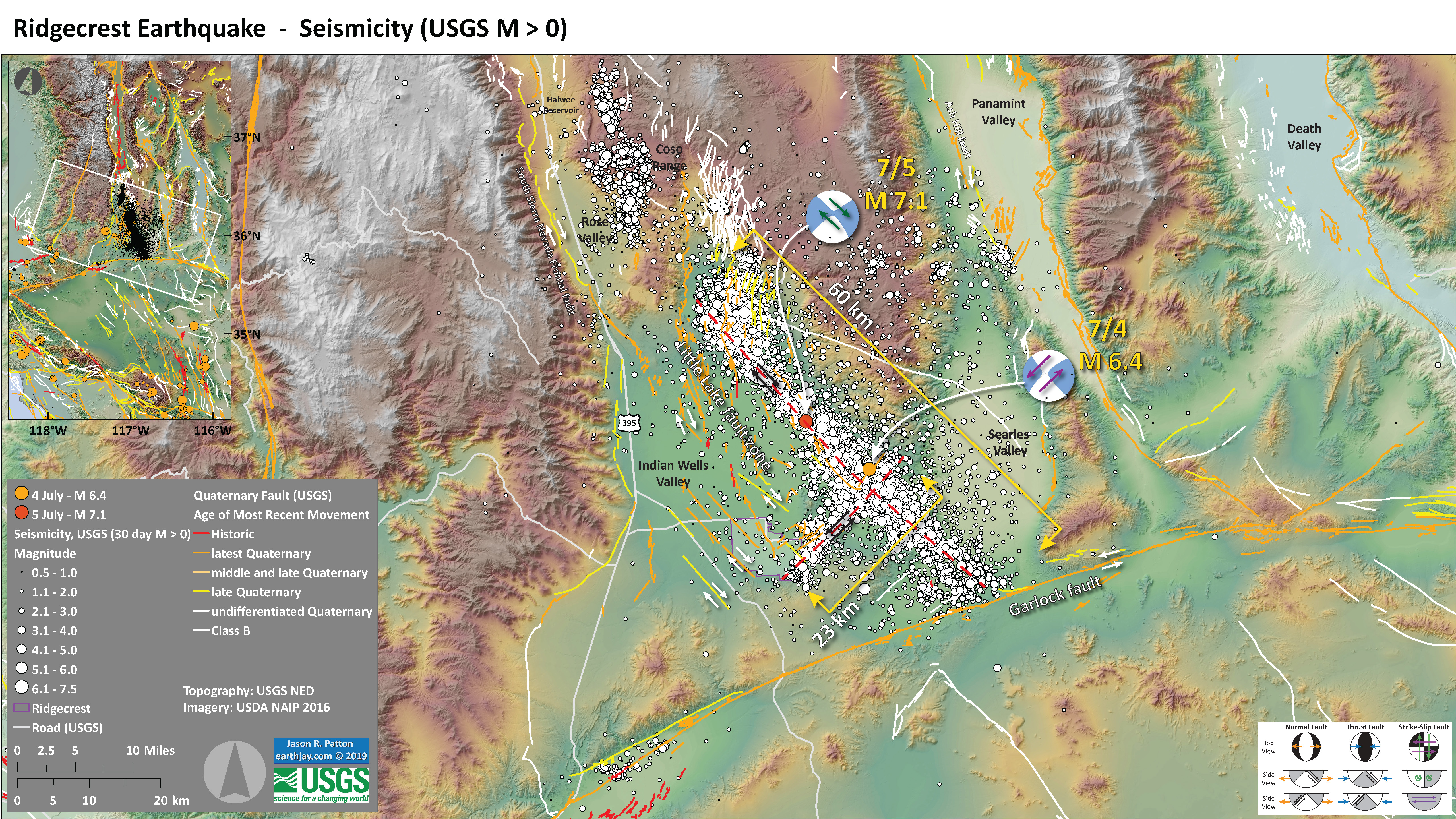
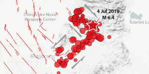
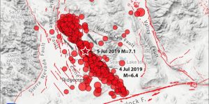
- Here is an updated seismicity map. There are two main types of earthquakes on this map. I present this map both with aerial imagery and with a topographic (“hillshade”) basemap. I outline the general area of Ridgecrest in purple.
- First, there are an abundance of aftershocks aligned with the two main faults that ruptured during this sequence (the northwest trending M 7.1 fault and the northeast trending M 6.4 fault). Part of the northwest striking fault ruptured during the M 6.4 event.
- Second, there are several areas that show earthquakes that were triggered by this sequence. There are some triggered earthquakes along the Coso Range (where the Coso Geothermal Field is located), some events along the Garlock fault, and some temblors along the Ash Hill fault (in Panamint Valley, to the north of Searles Valley).
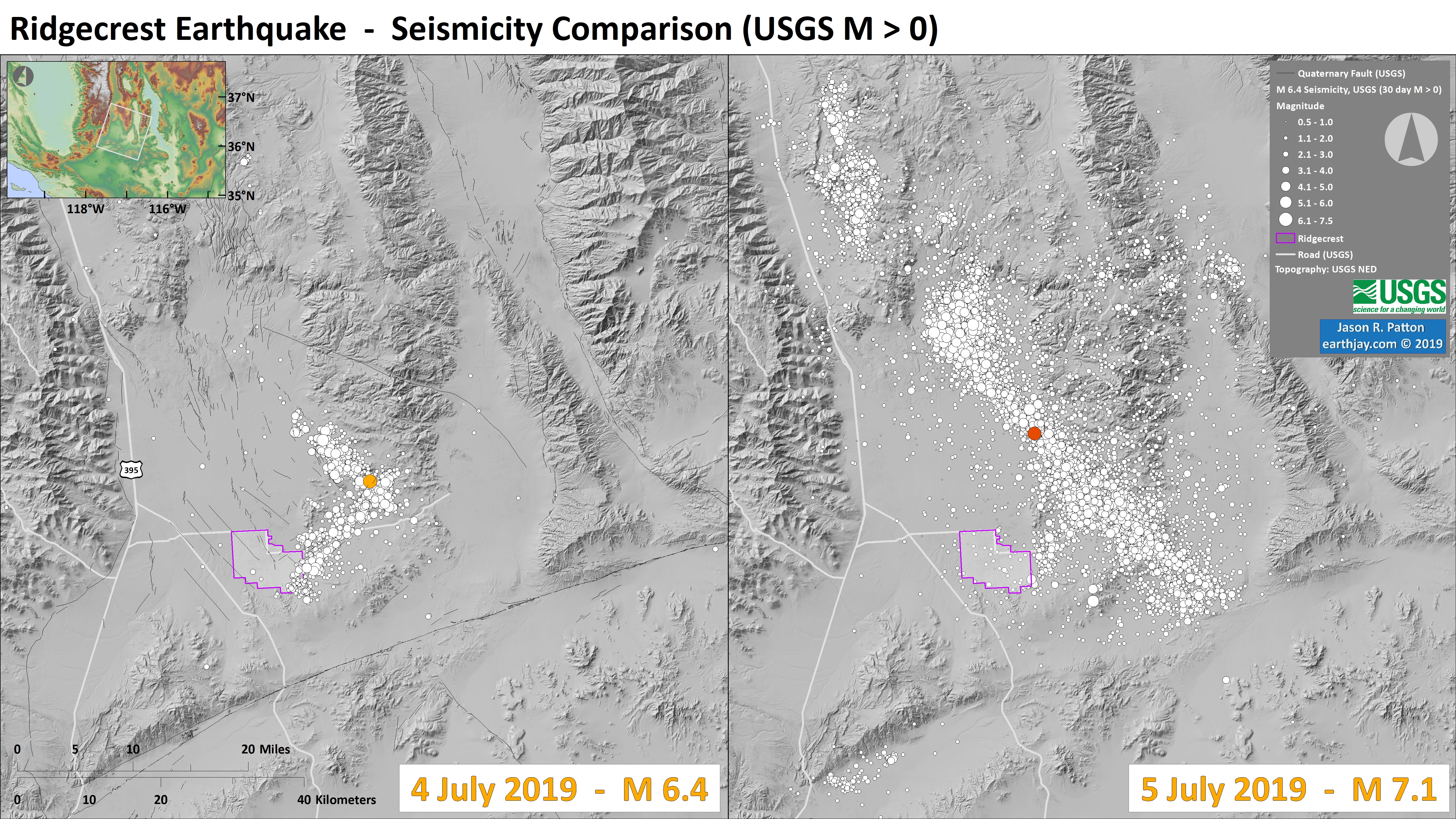
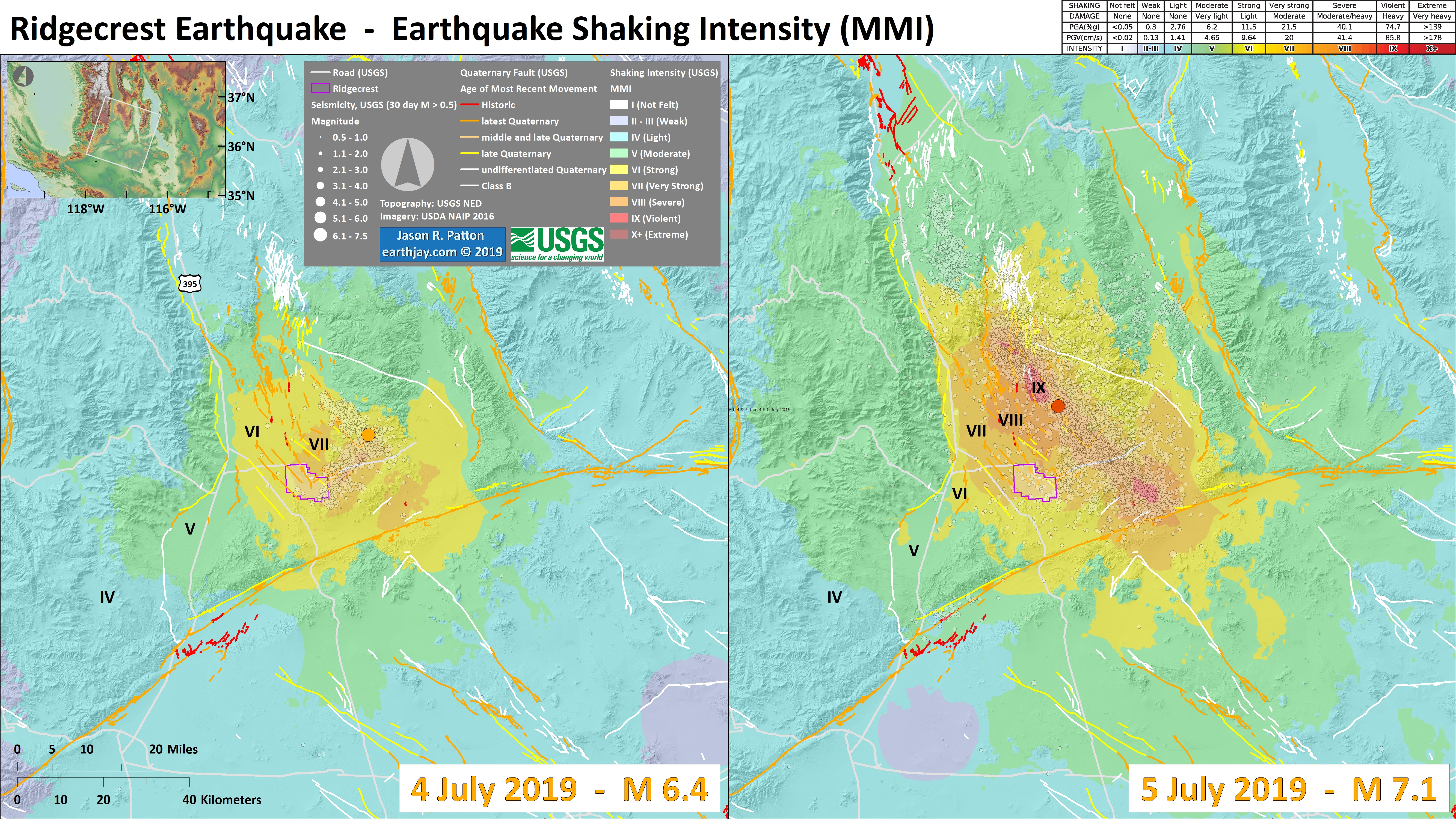
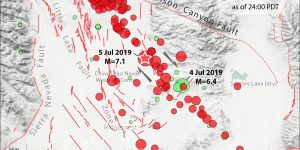
- This is a seismicity comparison for the two earthquakes. on the left are earthquakes (USGS) from prior to the M 7.1 earthquake and on the right are quakes after and including the M 7.1 temblor. I plot the USGS Quaternary fault and fold database on the left as black lines.
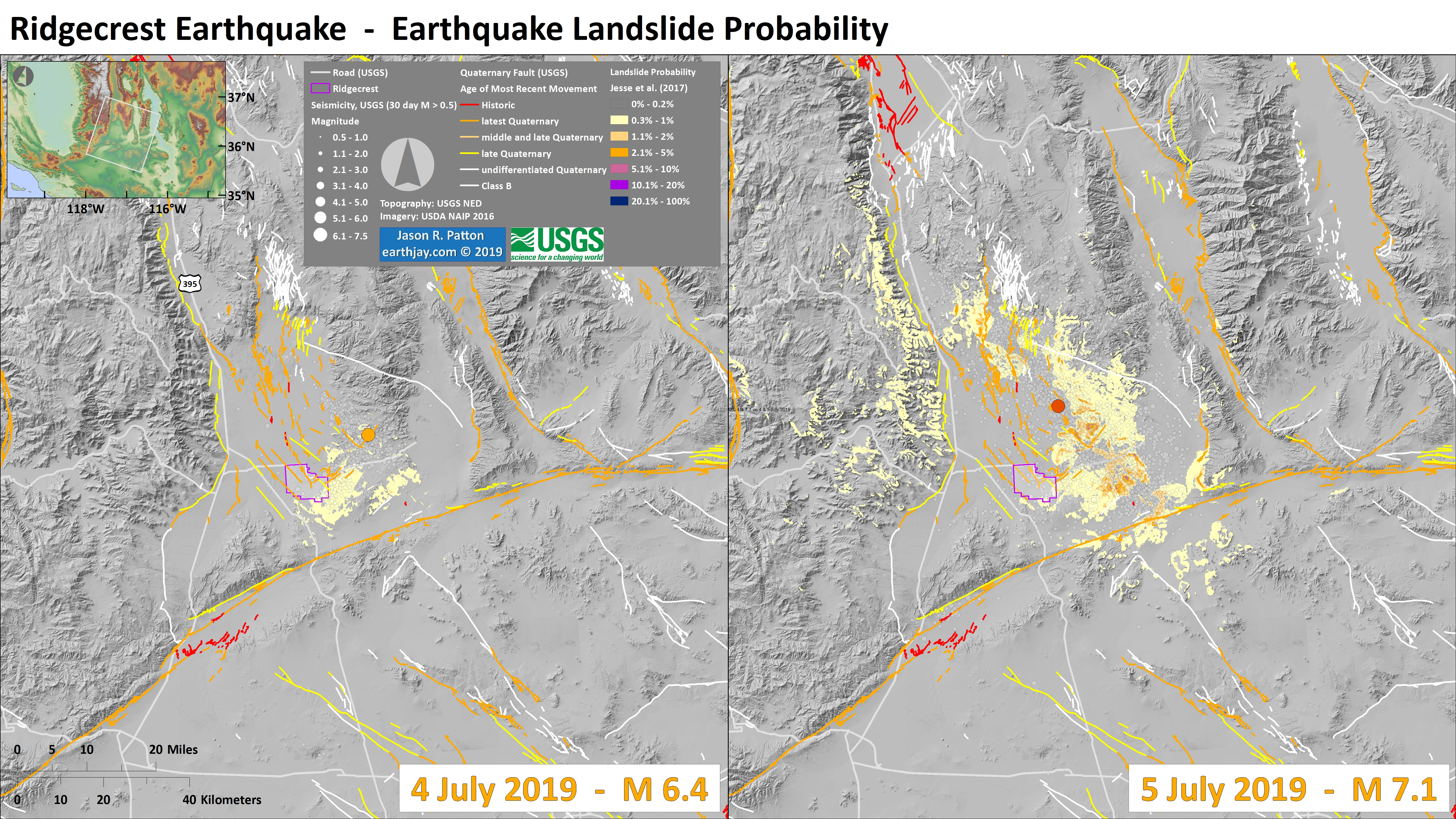
- Here is a map with landslide probability on it. Please head over to that report for more information about the USGS Ground Failure products (landslides and liquefaction). Basically, earthquakes shake the ground and this ground shaking can cause landslides. We can see that there is a low probability for landslides. However, we have already seen photographic evidence for landslides and the lower limit for earthquake triggered landslides is magnitude M 5.5 (from Keefer 1984-ish).
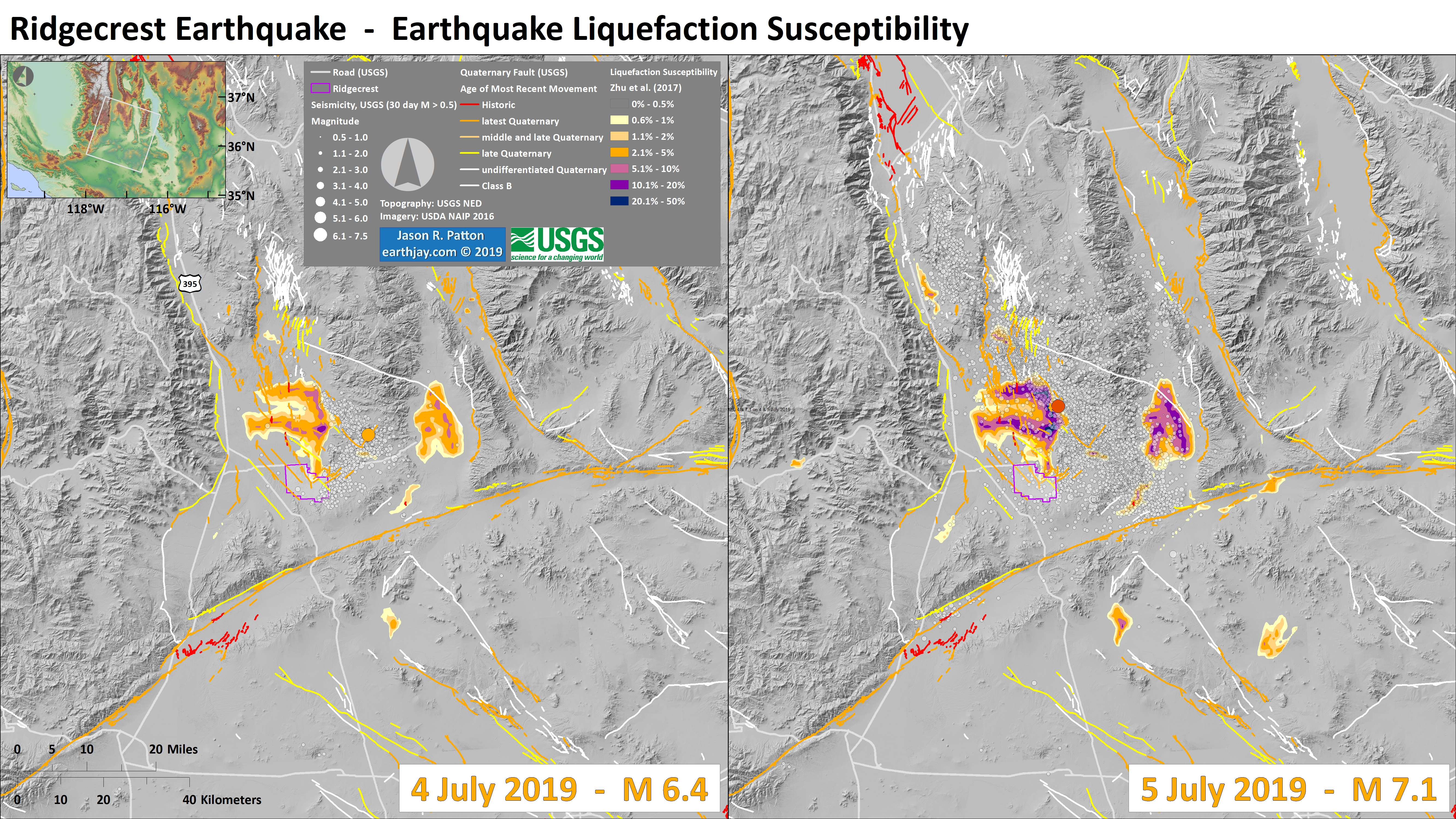
- Here is a map showing liquefaction susceptibility. I explain more about this type of map in my original report for the M 6.4 earthquake. Scroll down a bit to find the landslide and liquefaction maps for that event.
- Finally, here is a map that shows the shaking intensity for the M 6.4 and M 7.1 earthquakes. As I mention in my original report, this is based on a model that relates earthquake shaking intensity with earthquake magnitude and distance from the earthquake. Note that there was violent shaking from the M 7.1 event (MMI IX).

NASA JPL ARIA Data Products
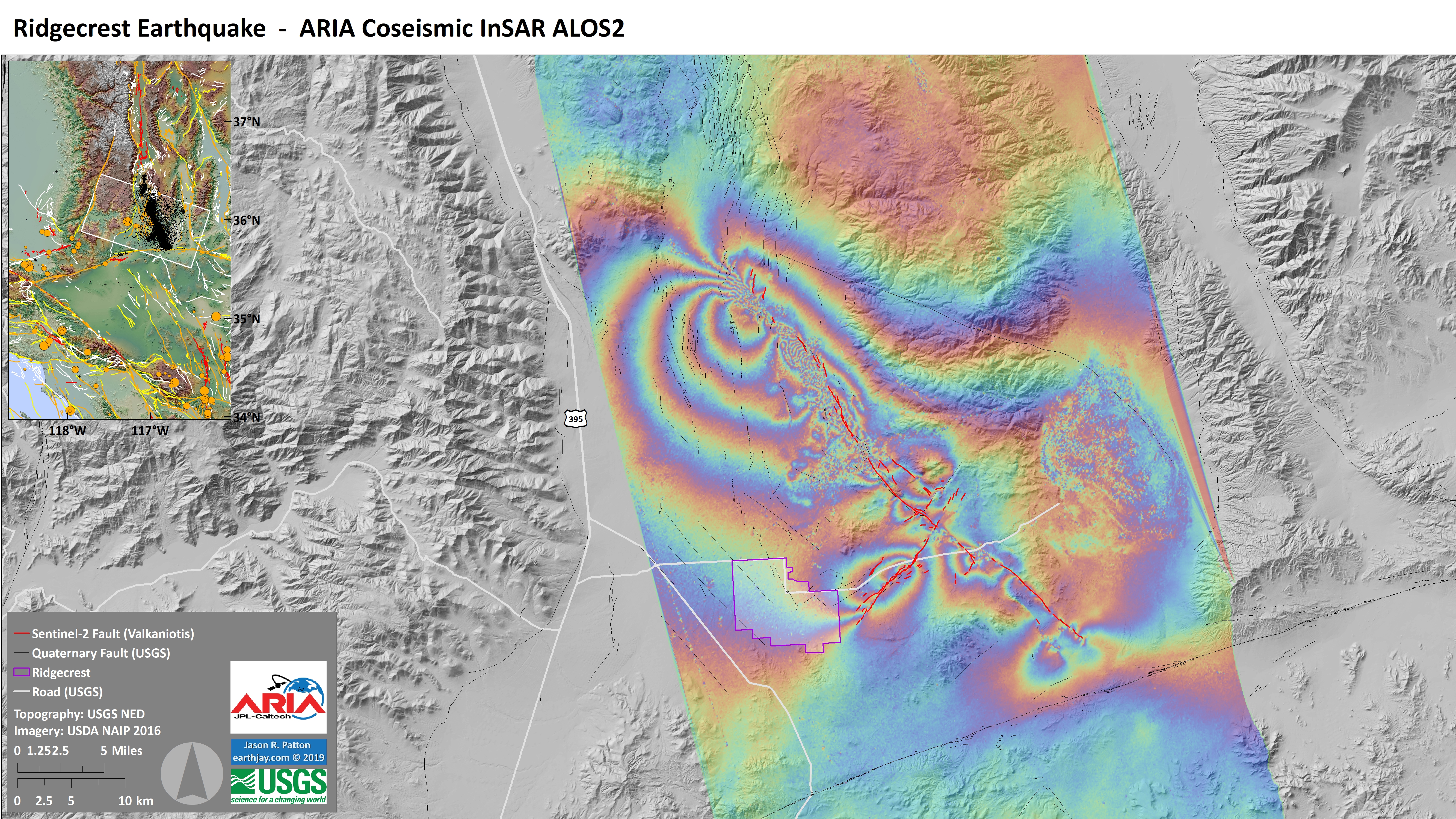
- NASA Jet Propulsion Laboratory (JPL) prepares Advanced Rapid Imaging and Analysis (ARIA) data products for major events worldwide. Their data are presented online here. I used the data from this event in a GIS computer program, but the data are prepared in Google Earth files too (so everyone can use them if they have a modern computer with an internet connection). This is a valuable government service.
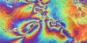
- This first map shows the results of modeling Synthetic Aperture Radar Interferometry data. Basically, Radar satellite imagery data from before and from after the earthquake are compared to model the amount of ground deformation that occurred between the satellite acquisitions. Each color band represents a certain amount of motion. This is referred to as the wrapped image.
- Here are a series of sources of background information about InSAR analysis.
- Wikimedia
- Centre for the Observation and Modeling of Earthquakes, Volcanoes, and Tectonics
- Geoscience Australia
- USGS
- Webinar for InSAR Analysis: NASA
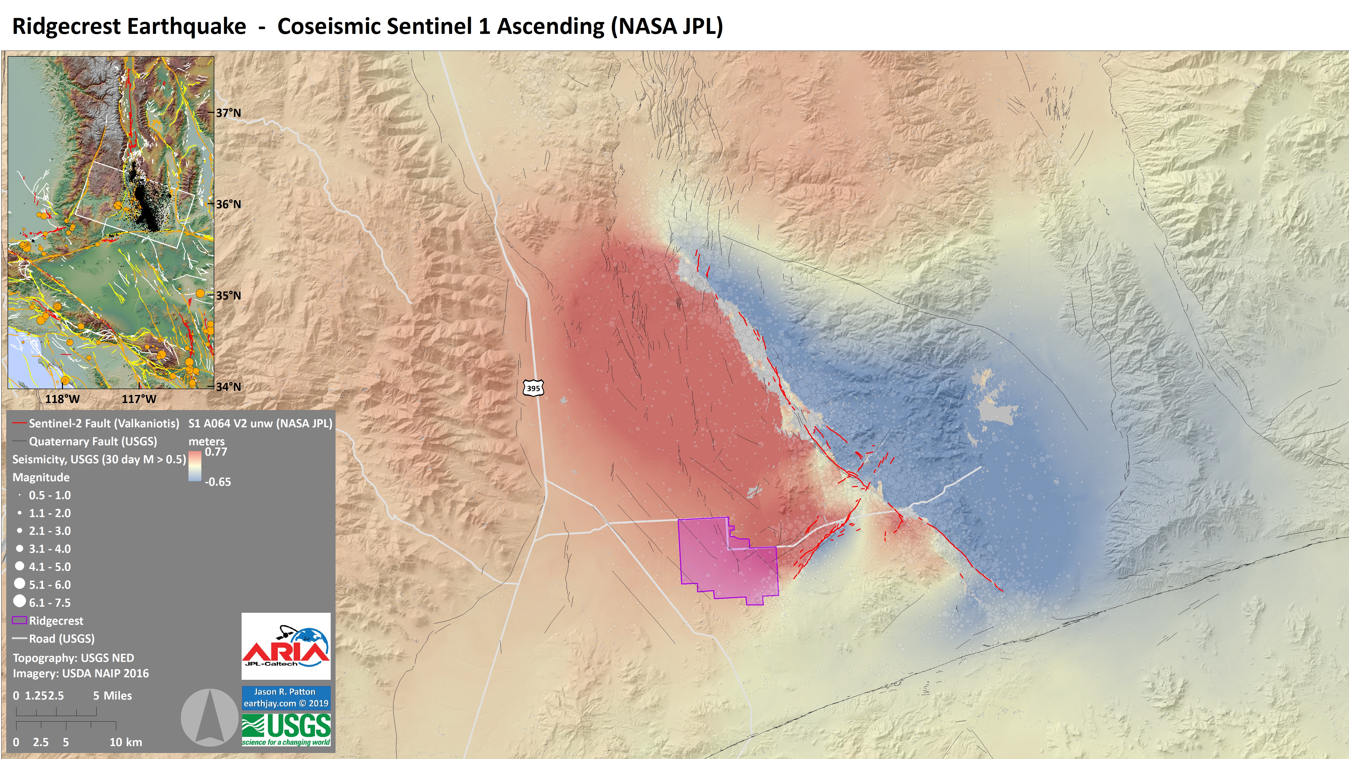
- This map is made using the same basic data, though it has been processed in a way to show the overall ground motion with just two colors, instead of color bands. This is called the unwrapped image.
- Below is the first in a series of videos that explains more about SAR and InSAR analyses.
Dr. Sotiris Valkaniotis
- Dr. Valkaniotis is a Greek geologist who has a great set of remote sensing skills who studies earthquake geology and paleoseismology. I include lots of social media posts below where people share their analyses. However, I select two images from Dr. Valkaniotis for this earthquake. Contact him for more information about his processing. As embedded below in the social media section, here is the tweet that is the source of these two maps.
- These images are similar to the NASA JPL ARIA unwrapped maps above. I include his description below in blockquote.
- Here is a map that Dr. Valkaniotis prepared showing fault lines he has interpreted from his model results.

Gradient render from unwrapped LOS displacement map (higher quality 20m from SNAP). Surface ruptures (major & minor) are easily visible as dark linear features (high displacement gradient). Processing in @esa_gep. Descending pair from #Sentinel1, #Ridgecrestearthquake

And the ascending pair from #Sentinel1, #Ridgecrestearthquake. Gradient render from unwrapped LOS displacement map (higher quality 20m from SNAP). Processing in @esa_gep.

Complex and detailed pattern of co-seismic ruptures for the #RidgecrestEarthquake sequence. Red lines are primary & secondary surface ruptures, together with small triggered ruptures away from main faults. Previously mapped Quaternary Faults with yellow, for comparison.
PBS News Hour: 2019.07.08
Death Valley at Devil’s Hole
The clip shows water violently sloshing around, rising and falling 10 to 15 feet, according to a park estimate. The video captures two angles, one looking into the cave and the other underwater inside it.
Devils Hole is a part of the desert uplands and spring-fed oases that make up the Ash Meadows complex, a national wildlife refuge.
Temblor Articles
Ross Stein (Ph.D.), Volkan Sevilgan (M.Sc.), Tiegan Hobbs (Ph.D.), Chris Rollins (Ph.D.), Geoffrey Ely, (Ph.D.), and Shinji Toda (Ph.D.) are coauthors to a suite of 5 articles presented on Temblor.net. Temblor is a National Science Foundation funded organization that promotes earthquake insurance and seismic retrofits for people in earthquake country. I wrote several articles for Temblor prior to starting work at the California Geological Survey. (My efforts at earthjay.com are purely volunteer and do not reflect endorsement nor review from or by CGS.)
These reports are excellent sources of interpretive information at the detail for non experts (sometimes my reports are at a detail more aimed towards undergraduate geology students, though I attempt to make them available to a broad audience as well). I include a few figures from their reports that I find most interesting, but please check out their articles for more information!
- Dr. Stein begins by presenting an hypothesis that these earthquakes are in a region of increased tectonic stress following the 1872 Owens Valley Earthquake, estimated to have a magnitude of M 7.6 (though it happened prior to modern seismometer instrumentation, so magnitude estimates have considerable uncertainty).
- When earthquake faults slip, the surrounding crust is squished and squashed. This deformation changes the tectonic stresses in the crust. In some places this change causes an increase in the amount of stress on earthquake faults and in some places it decreases the tectonic stress. In places where the stress increases, the fault is brought closer to having an earthquake, and vice versa for places where the stress is diminished.
- These stress changes are very small, so for a fault to be triggered by these changes in “static coulomb stress,” the fault had to be almost ready to slip before these changes happened. More can be found in Stein (2003) and Toda et al. (2005) linked below in the references.
- In the map below, warm colors represent areas with an increase in (static coulomb stress) and cool colors represent a decrease in stress. I include their figure caption in blockquote below the figure (as for all their figures).
![]()
he site of the July 4th shock was likely brought closer to failure in the 1872 M~7.6 shock. Notice that the (red) stress trigger zones of the this 148-year-old quake are all seismically active today, whereas the (blue) stress shadows are generally devoid of shocks.
- The Owens Valley fault triggering is speculative of course, since that earthquake was so long ago. However, there are other cases where aftershocks or triggered earthquakes are happening a long time after the main event. For example, there are ongoing aftershocks following an 1872 earthquake near Lake Chelan (Bakun et al., 2002; Brocher et al., 2018).
- Stein and his colleagues calculated “static coulomb” stress changes imparted by the Ridgecrest Earthquake Sequence onto a series of other faults in the area. Read more about their analyses here.

Here we calculate stress transferred to the principal mapped faults, using the USGS slip model for the 7.1 and a model based on University of Nevada Reno GPS displacements for the 6.4 (not shown here for simplicity, but included). Most of the stress change is from the 7.1: it was several times larger than the 6.4 and torqued the surrounding crust far more. This fault inventory might be woefully incomplete, of course: the 7.1 itself struck on an unmapped fault. Nevertheless, the most striking result is the >2-bar stress increase on a 30-km (20-mile) section of the Garlock Fault. An end-to-end rupture on the Garlock, if (still) possible, would be in the magnitude 7.6-7.8 range.
- In my interpretive posters above, I mention the areas where there have been triggered earthquakes (e.g. the Coso Geothermal Field, the Garlock fault, the Ash Hill fault). Turns out, Stein and his colleagues were thinking the same thing.
- They prepared a figure in their report here where they show changes in “static coulomb” stress. They label the same areas I mention (except the Ash Hill fault in Panamint Valley). Take a look at the areas of increased stress compared to these three regions (even the Ash Hill fault is in an area of increased stress).

Faults in the red lobes are calculated to be brought closer to failure; those in the blue ‘stress shadows’ are inhibited from failure. The calculation estimates what the dominant fault orientations are around the earthquakes by interpolating between major mapped faults (shown in red lines). So, we would expect strong stressing in the Coso Volcanic Field to the north (where the aftershocks lie), and along the Garlock Fault to the south (but not where most of them lie).
- Hobbs and Rollins speculate that the San Andreas fault may also have changes in (static coulomb) stress imparted by the Garlock fault if that were to slip. Read more in their article here.
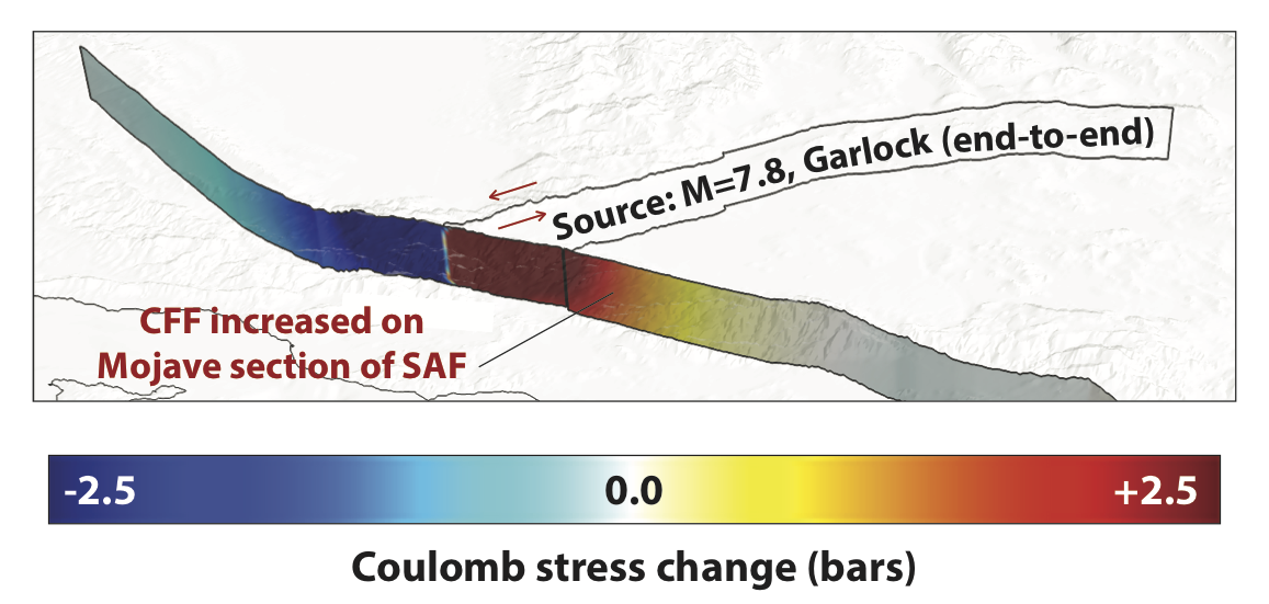
If the western and central Garlock were to rupture, it would load the section of the San Andreas just north of Los Angeles. The jog in the San Andreas under the S in “Source” is at Palmdale. Figure from McAuliffe et al. [2013].
Below are all the Temblor articles to read
 |
2019.07.04 Southern California M 6.4 earthquake stressed by two large historic ruptures |
 |
2019.07.05 Earthquake early warning system challenged by the largest SoCal shock in 20 years |
 |
2019.07.06 Magnitude 7.1 earthquake rips northwest from the M6.4 just 34 hours later |
 |
2019.07.06 M 7.1 SoCal earthquake triggers aftershocks up to 100 mi away: What’s next? |
 |
2019.07.09 The Ridgecrest earthquakes: Torn ground, nested foreshocks, Garlock shocks, and Temblor’s forecast |
- Here are the references for these Temblor articles.
- Stein, R. S., and Sevilgen, V., (2019), Southern California M 6.4 earthquake stressed by two large historic ruptures, Temblor, http://doi.org/10.32858/temblor.034
- Hobbs, T.E. and Rollins, C., (2019), Earthquake early warning system challenged by the largest SoCal shock in 20 years, Temblor, http://doi.org/10.32858/temblor.035
- Ross S. Stein, Tiegan Hobbs, Chris Rollins, Geoffrey Ely, Volkan Sevilgen, and Shinji Toda, (2019), Magnitude 7.1 earthquake rips northwest from the M6.4 just 34 hours later, Temblor, http://doi.org/10.32858/temblor.037
- Ross S. Stein, Chris Rollins, Volkan Sevilgen, and Tiegan Hobbs, (2019), M 7.1 SoCal earthquake triggers aftershocks up to 100 mi away: What’s next?, Temblor, http://doi.org/10.32858/temblor.038
- Chris Rollins, Ross S. Stein, Guoqing Lin, and Deborah Kilb (2019), The Ridgecrest earthquakes: Torn ground, nested foreshocks, Garlock shocks, and Temblor’s forecast, Temblor, http://doi.org/10.32858/temblor.039
Field Photos
- Below are some field photos I took. I cannot tell anyone where they were taken (at least not yet) as we don’t have clearance. I may post more later, but wanted to post some to show people the type of observations we were making.
- This is Dr. Chris DuRoss (USGS) as we walked across the scarp at our first site working together.
- Here is a great one of Dr. Jessie T. Jobe (USGS, soon to be USBR) taking notes at that same scarp (DuRoss’ boots for scale).
- This is a portion of a road where the fault crossed. There were several dm of lateral offset on either side of the road, but the road itself had an imperceptible amount of lateral offset (i.e. 1 ± 1 cm offset). There was some amount of compression here.
- Here we were projecting the ground surface across the fault to estimate the amount of vertical displacement. Dr. Ryan Gold (USGS) is measuring while a Navy Base geologist is holding the profile stick along the ground surface.
- Here is a photo very similar to Mr. Brian Olson’s tweeted photo, but I took this one instead. Dr. Belle Philibosian (USGS) is on the left and Kelly (NAWCL geologist) is on the right. This shows right-lateral strike-slip displacement of 420 cm. We thought nobody would believe us, so we made another measurement nearby to confirm.
- I located some beautiful slickenlines (grooves in the fault surface created when the fault slips) and this is Dr. Beth Haddon (USGS) collecting strike, dip and rake data for these lines. We collected many photos of this site so that we can create a 3-D model (using structure from motion).
- Here is Dr. Belle Philibosian looking spectacular as usual, providing scale to help us understand the amount of vertical separation across the fault in this location.
- We located some evidence for liquefaction too. Here is a sand volcano, where lots of the sediment got washed away by the fluid that possibly shot up through this hole.
- This was a great opportunity to show the compass orientation of these conjugate fault offsets in the road. The road material properties probably controlled the location of the faults here (there were pre-existing planes of weakness as evidenced by the tar patches, but some of the pavement faulting was new).


- 1906.04.18 M 7.9 San Francisco
- 2017.12.14 M 4.3 Laytonville
- 2016.11.06 M 4.1 Laytonville, CA
- 2016.11.03 M 3.8 Laytonville, CA
- 2016.08.10 M 5.1 Lake Pillsbury, CA
- 2015.08.30 M 3.6 Mendocino County, CA
- 2015.07.27 M 3.5 Point Arena, CA
- 2018.07.30 M 3.7 San Pablo Bay
- 2018.01.04 M 4.4 Berkeley
- 2019.07.04 M 6.4 Ridgecrest
- 2019.07.05 M 6.4 / 7.1 Ridgecrest Update #1
- 2019.07.18 M 6.4 / 7.1 Ridgecrest Update #2
- 2019.07.20 M 6.4 / 7.1 Ridgecrest Update #3
- 2016.02.23 M 4.9 Bakersfield
- 2015.12.30 M 4.4 San Bernardino, CA
- 2015.05.03 M 3.8 Los Angeles, CA
- 2015.04.13 M 3.3 Los Angeles, CA
- 2014.04.01 M 5.1 La Habra p-3
- 2014.03.29 M 5.1 La Habra p-2
- 2014.03.28 M 5.1 La Habra p-1
- 2016.08.04 M 4.5 Honey Lake, CA
San Andreas fault
General Overview
Earthquake Reports
Northern CA
Central CA
Southern CA
Eastern CA
- 2019.06.05 M 4.3 San Clemente Island
- 2018.04.05 M 5.3 Channel Islands
- 2018.04.05 M 5.3 Channel Islands Update #1
- 1994.11.17 M 6.7 Northridge, CA
- 1971.02.09 M 6.7 Sylmar, CA
Southern CA
Earthquake Reports
Social Media
Here's some context for the M7.1 #earthquake today in California and its foreshock/aftershock sequence. It is well off the San Andreas Fault and north of the Garlock fault in the Eastern California Shear Zone. Read more from @Temblor about this area here: https://t.co/thInzw8ghF pic.twitter.com/NpLvDpyn1y
— Dr. Kasey Aderhold (@kaseyaderhold) July 6, 2019
SLIPNEAR model along the aftershocks of the M6.4 mainshock. Slip inversion carried out with 2 different fault planes, one SE dipping (strike 45) from FMNEAR, and the other NW dipping from GCMT (strike 228). Slip distribution is quite similar in both cases (main slip zone stable) pic.twitter.com/gegZ9BSqR9
— Bertrand Delouis (@BertrandDelouis) July 7, 2019
Cumulative stress change caused by 4 July 2019 M=6.4 and the 7 July 2019 M=7.1 earthquakes on nearby strike slip faults, the red color represents increase seismic hazard Dr Kariche@IPGS2019 #RidgecrestEarthquake @DrLucyJones pic.twitter.com/jpGfqKhdzD
— Jugurtha Kariche (@JkaricheKariche) July 7, 2019
Pixel tracking of @Planetlabs satellite images reveals the northern termination of the Mw 7.1 July 5th #earthquake. Result shows only ~16 km of rupture, with a minor transtensional splay in lower right. Slip profile, exhibits classic ‘dogtail’ taper. pic.twitter.com/S5CfsKd5AP
— Chris Milliner (@Geo_GIF) July 7, 2019
A complete image of the Mw 7.1 Ridgecrest #earthquake showing amount of surface displacement measured by @planetlabs satellite imagery. Rupture is ~40 km in length with up to ~5m of fault slip. Fault trace has remarkably similar rupture geometry to 1999 Mw 7.1 Hector Mine event. pic.twitter.com/ORBA5D0gKz
— Chris Milliner (@Geo_GIF) July 8, 2019
Came across this sandy vegetation mound out on the China Lake bed, which was cut in half by the fault rupture. Measured offset is approximately 8 feet. #earthquake #Ridgecrest pic.twitter.com/ok95QmfZQ8
— Brian Olson (@mrbrianolson) July 8, 2019
Estimated preliminary extent of the main rupture of Mw7.1 #earthquake #Ridgecrest CA, combining surface rupture traces from @CATnewsDE and @Geo_GIF (traced on @planetlabs imagery). Main rupture (red) extends at >45km. Black dots: reviewed epicenters USGS. Quaternary Faults: USGS. pic.twitter.com/Yq68sg86ub
— Sotiris Valkaniotis (@SotisValkan) July 8, 2019
Great day mapping. Even made a 2 second cameo on PBS News hour. ;)
@patton_cascadia@FaultyAndSalty#RidgecrestEarthquake https://t.co/kkDR4WP2ib— Nick Graehl (@nickgraehl) July 9, 2019
As promised, here are pictures of formerly high-speed dirt and environs! Enjoy these annotated photos from our recon mapping with J. Dolan and S. Attia yesterday of the Searles Valley EQ seq. near Ridgecrest, CA. Please contact me for more photos and information-ahatem@usc.edu pic.twitter.com/jZSIEaJuZY
— Alex Hatem (@pride_of_lowell) July 9, 2019
A few more! pic.twitter.com/OckTe5LSx7
— Alex Hatem (@pride_of_lowell) July 9, 2019
OK, this really is the last one. The M6.4 earthquake strikes almost perpendicular to the track direction, and shows a deformation pattern that is more symmetric. We are mostly seeing the E-W movement of the fault in this case.
[Thanks to @JAXA_en for a great radar satellite!] pic.twitter.com/joFeJ5tURk
— Gareth Funning (@gfun) July 9, 2019
#RidgecrestQuake from Space
This colorful map shows surface changes from the two earthquakes that rattled California last week. More here: https://t.co/qnj4B8zJm8 pic.twitter.com/w44MXwd3xL
— NASA JPL (@NASAJPL) July 9, 2019
Some photos from today…#RidgecrestEarthquake pic.twitter.com/x5HrsdpJc6
— Nick Graehl (@nickgraehl) July 9, 2019
Surface rupture & displacement from the Mw 7.1 #Ridgecrest #earthquake CA as seen from #Sentinel2 images from @CopernicusEU. Animation using June 28 and July 8 images. Optical correlation map to follow later. pic.twitter.com/4cW0ovSIcM
— Sotiris Valkaniotis (@SotisValkan) July 9, 2019
Quake ripped right through the flattest parts of the basin with maybe a little compression ridge in the southern stepover pic.twitter.com/NnSmKa3kSv
— Bill Barnhart (@HawkeyeSeismo) July 9, 2019
It was a boots on the ground kind of day for CGS and USGS. Today we focused on measuring fault rupture offsets on the China Lake NAWS base #faultmapping #earthquake #Ridgecrest @CalConservation pic.twitter.com/L2PTZZF3ed
— Ellie Spangler (@EllieSpangler) July 9, 2019
Data available; high-resolution figures and raster files for subpixel co-seismic offsets for the Mw6.4 and Mw7.1 #Ridgecrest, California #earthquakes, using #Sentinel2 images. #MicMac and CosiCorr files. Files uploaded in Zenodo repository: https://t.co/l10csPV4n7 pic.twitter.com/1MQIeeEzFj
— Sotiris Valkaniotis (@SotisValkan) July 9, 2019
More from our #RidgecrestEarthquake coverage: DOC Drone footage south of Ransberg Road captures surface rupture. Photo: Roadway surface displacement – right-lateral offset approx. 6.5 ft and 3' vertical. Offset bottom of pic 5' ~ Footage: Nathaniel Roth. Photo: @mrbrianolson pic.twitter.com/6kDX8Tcc1e
— DeptofConservation (@CalConservation) July 10, 2019
Surface fault ruptures from the July 4th Mw6.4 #Ridgecrest #earthquake visible using #Sentinel2 optical (normalized difference – Band4) and #Sentinel1 interferogram (made with SNAP at @esa_gep). Multiple traces, marked with orange arrows pic.twitter.com/70ePXUsiQD
— Sotiris Valkaniotis (@SotisValkan) July 10, 2019
The Ridgecrest earthquakes: Torn ground, nested foreshocks, Garlock shocks, and Temblor’s forecast | https://t.co/1twVj9F84q https://t.co/x6aHPj0Az0 via #NSFfunded @temblor #California #Earthquake
— temblor (@temblor) July 10, 2019
Azimuth phase gradient map, Range phase gradient map, Zoom in of range phase gradient map. It is filled with cracks!!!! #RidgecrestEarthquake pic.twitter.com/pJ5ydG5xR0
— Xiaohua Xu (@XiaohuaXu1) July 10, 2019
#Ridgecrest #Trona #earthquakes
M≥2.0 2019-07-04>2019-07-10-09h https://t.co/sRUqn89xEO relocations w/ station corrections, over ALOS-2/JAXA/@NASAJPL-ARIA interferogram https://t.co/NpRQTwvQn8
Events colored by origin time before & after M7 mainshock (left), & by depth (right) pic.twitter.com/GnOO4kYR0K— Anthony Lomax 🌍🇪🇺 (@ALomaxNet) July 10, 2019
Track 64 interferogram from Sentinel-1 data acquired by @esa. Remind me of the Hector Mine interferogram. #RidgecrestEarthquake #ridgecrestearthquakes pic.twitter.com/oqDQa5qC6e
— Xiaohua Xu (@XiaohuaXu1) July 10, 2019
Following #Ridgecrest earthquake, @NASAJPL ARIA ALOS-2 interferogram, appears to show very small triggered slip on the Garlock fault. Bottom shows USGS Quaternary fault trace. pic.twitter.com/kppDaIkpsD
— Chris Milliner (@Geo_GIF) July 9, 2019
I saw some spectacular faulting while putting in extra seismometers around Ridgecrest. pic.twitter.com/aOXz9aaNnY
— Elizabeth Cochran (@escochran) July 10, 2019
Ken Hudnut (USGS), along w/partners Bob Fenton (FEMA Region IX Admin.) and Mark Ghilarducci (Director of CalOES) briefed @VP about the M7.1 earthquake that struck CA on July 5, 2019. Emphasis was placed upon coordination between CGS, USGS and @USNavy. https://t.co/suTpYkbe5z pic.twitter.com/lrSXC04T8W
— USGS (@USGS) July 11, 2019
A preliminary semi-realistic finite element model of M6.9 Ridgecrest EQ, with fault curvature following pixel-tracked trace, CVM-H tomography, topography. Vertical fault is set for this stage. Green's function library on its way. @SotisValkan @chandraphyctc @shirzaei @ratlab3 pic.twitter.com/WSd9520fiT
— Jay Tung (@jaytung_earth) July 11, 2019
Thanks to incoming InSAR images covering the complete rupture (below ALOS-2 interferogram from the @NASAJPL ARIA project), the information value provided by previous rapid slip inversions using strong motion data (SLIPNEAR) can be evaluated: pic.twitter.com/KDTC45kKuP
— Bertrand Delouis (@BertrandDelouis) July 10, 2019
Map of permanent ground displacement due to M6.4 and M7.1 earthquakes near Ridgecrest California from NASA Caltech-JPL ARIA processing of JAXA ALOS-2 (unwrapped interferogram, path 65). This InSAR sensitive to west and up motion of ground. @zross_ relocated main and aftershocks pic.twitter.com/CuGtOv78nB
— Eric Fielding (@EricFielding) July 10, 2019
Our Automatic Sentinel1 processing of co-seismic interferogram for the California Earthquakes with Mw. 7.1 and Mw 6.4 (Interferogram and LOS Displacement map) using #Sentinel1 @ESA_EO @CopernicusEU Track 64 (20190704-20190710) #IREA #CNR @FraxInSAR @claudiodeluca @VDN75 pic.twitter.com/ruGHFoQ0pv
— Fernando Monterroso (@maferp_13) July 10, 2019
Left lateral faulting #SoCalEarthquake #drone #Ridgecrest #California pic.twitter.com/7QHGGXGm7G
— Forrest Lanning (@rabidmarmot) July 11, 2019
#Sentinel2 mapped co-seismic #fault traces from the #Ridgecrest CA #earthquakes. While Sentinel-2 (Band 4 normalized difference) offers extravagant detail at certain parts, is missing traces in other areas. Interesting when in comparison with other sensors/methods & field. pic.twitter.com/VCb8ghN8WM
— Sotiris Valkaniotis (@SotisValkan) July 11, 2019
My first look at #RidgecrestEarthquake rupture on Tues and first tweet ever!! pic.twitter.com/QFOpokctQR
— Stephen Angster (@faultjumper) July 11, 2019
Found our BIGGEST offset yet for the fault that caused the M7.1 earthquake. This channel is offset about 13 feet! #ridgecrestearthquake #earthquake #ridgecrest pic.twitter.com/EQCh3Z9DBj
— Brian Olson (@mrbrianolson) July 12, 2019
An amazing week working with colleagues from @CalConservation California Geological Survey and the @usgs mapping ruptures from the earthquakes in Ridgecrest. Thanks to the residents who have been welcoming and the @USNavy for incredible logistical support. #ridgecrestearthquakes pic.twitter.com/Yqs8yAZtLY
— Tim Dawson (@timblor) July 12, 2019
This animation shows preliminary results from precise relocation of the Ridgecrest foreshock sequence, up to the the time of occurrence of the M 7.1 mainshock. Full details at: https://t.co/Gm3GuSPt0s pic.twitter.com/RfIijTiHfu
— USGS (@USGS) July 12, 2019
A very preliminary fault slip model for #RidgecrestEarthquake, using data from GPS, @esa Sentinel-1, @ALOS2_JAXA, optical imagery from @planetlabs by @Geo_GIF. Model, surface displacement and Coulomb stress available at https://t.co/SSyQaHdJYh. pic.twitter.com/TZ8PQop7cZ
— Xiaohua Xu (@XiaohuaXu1) July 12, 2019
CGS and USGS teams mapped fault offsets that were an order of magnitude less than yesterday’s, but in someways much cleaner to measure. Here is a shrub dune left-laterally offset 30 cm by the July 4 M 6.4 pic.twitter.com/F7UH6f82An
— Tim Dawson (@timblor) July 13, 2019
Updated rupture map of #Ridgecrest earthquake. Faults mapped from @Planetlabs offsets, and Sentinel-1 wrapped and phase gradient. Juncture of Mw 6.4 and 7.1 is highly complex.
Green = primary fault rupture
Red = secondary faults
Blue dots = aftershocks (SCSN) pic.twitter.com/N3TSO02GYA— Chris Milliner (@Geo_GIF) July 12, 2019
This one woke me up:
Today's M4.9 aftershock was recorded by a temporary seismometer at ~2 km epicentral distance. It recorded a peak acceleration of 14%g. Intensities in Ridgecrest imply accelerations in the same range, or maybe even higher locally. This illustrates an important point. pic.twitter.com/ruefagOhdT
— Susan Hough (@SeismoSue) July 13, 2019
Headed home after a week working on response to #RidgecrestEarthquake. Impressive effort by all involved from #USGS #CGS #UNR #EERI and many more. A few of my favorite photos: ~4 m offset dirt road, 108F temps, central part of M7.1 rupture with @timblor and @chrisduross for scale pic.twitter.com/B8fIfaNxti
— Ryan Gold (@runr447) July 13, 2019
'NASA's ARIA Team Maps California Quake Damage' news article from the #NASA_App @NASAJPL https://t.co/Kyk34SmN6q
— Eric Fielding (@EricFielding) July 13, 2019
Growing evidence for Garlock fault having very small triggered slip. Both ALOS-2 wrapped phase and Sentinel 1 aziumuthal gradient map show small slip for ~35 km alongfault. @XiaohuaXu1 pic.twitter.com/bKSbGmWO9U
— Chris Milliner (@Geo_GIF) July 10, 2019
This @UNVACO map shows how GPS stations moved from just before to just after the #RidgecrestEarthquake. The arrows show the direction & size of motion. This represents how much the ground moved at each site. The scale arrow in the lower left represents 100 mm, or 10 cm (~4 in). pic.twitter.com/tQzvNGugms
— IRIS Earthquake Sci (@IRIS_EPO) July 8, 2019
The possible fault sources of the #ridgecrestearthquake by analytical solution combining #sentinel1 #sentinel2 @UNAVCO gps and @USGS faultlines data.
The path has just begun.@SimoneAtzori73 @maferp_13 @FraxInSAR @EugenioSansosti pic.twitter.com/F34nIjfZKL— Vincenzo De Novellis (@VDN75) July 13, 2019
Ground deformation after #Ridgecrest earthquake using #Sentinel1 ascending dataset. #RidgecrestEarthquake #RIKEN #RIKEN_AIP #Earthquake #Deformation pic.twitter.com/EFQadAoaZ7
— Sadra Karimzadeh (@Sadra_Krmz) July 13, 2019
Why historical seismology? Some years ago @Kate6HTN and I wrote a paper on the 1872 Owens Valley earthquake, presenting evidence that the rupture continued south of Lone Pine, to Haiwee. pic.twitter.com/VNND3HfniX
— Susan Hough (@SeismoSue) July 14, 2019
"Scientists from the USGS and other organizations continue field work and analyses". Here is a release of the surface rupture map:https://t.co/cC53bdzEQZ pic.twitter.com/tS3p5t9c6z
— Stéphane Baize (@stef92320) July 13, 2019
More results using @ALOS2_JAXA data available on https://t.co/SSyQaHdJYh . What really needed is the other look direction. Waiting for 16th Sentinel-1. Also check out the north west corner. That's central valley going down. pic.twitter.com/419xh9uJQi
— Xiaohua Xu (@XiaohuaXu1) July 14, 2019
Here it is. With @YorgosBz and @ESM_db we've been looking at the (possibly) impulsive features of ground motions from the #californiaearthquake, as identified by Baker's 2007 algorithm. Polygon is source projection, E is epicenter. (Note: just preliminary, no conclusions yet.) pic.twitter.com/4vucfl8nuV
— iunio iervolino (@iuniervo) July 14, 2019
Last 12 days on a seismogram ~15km S of #Ridgecrest showing:#Ridgecrest #Trona #earthquake
M6.4 2019-07-04 (green)
M7 2019-07-06 (black)
…and many, many aftershocks#Australia
M6.6 2019-07-14 (blue, lower left, 06h)#Indonesia
M7.3 2019-07-14 (blue, lower right) pic.twitter.com/vxnqPB8zd6— Anthony Lomax 🌍🇪🇺 (@ALomaxNet) July 15, 2019
Many are asking *why* Ridgecrest didn't suffer more damage from the M7.1 earthquake. I noticed the peak ground accelerations measured IN Ridgecrest were actually LESS for the M7.1 despite it releasing 11x more energy. pic.twitter.com/UyUGVYyNh0
— Brian Olson (@mrbrianolson) July 15, 2019
Wanted to say I was honored to join the team collecting location & offset data from recent Ridgecrest earthquakes. From huddling under tables w/ @kwhudnut & @earthquakemom during the M7.1 to sweating profusely on the dry lake bed, I valued all of it. #TeamCGS #TeamUSGS pic.twitter.com/Yxzf8yrQ15
— Brian Olson (@mrbrianolson) July 14, 2019
Another preliminary fault slip model for #RidgecrestEarthquake, using data from @esa #Sentinel1 and @UNAVCO GPS. @USGS faultlines (black) & @IRIS_EPO earthquakes distribution (red) are also shown; the darkest blue corresponds to ~5.5 m slip value.@SimoneAtzori73 @EricFielding pic.twitter.com/gSTzlTDD4X
— Vincenzo De Novellis (@VDN75) July 15, 2019
Well, at AGU it is going to be called:
"S041 – The 2019 M6.4 Searles Valley and M7.1 Ridgecrest Earthquakes"
Some improvement…https://t.co/adGovA3GyP— Anthony Lomax 🌍🇪🇺 (@ALomaxNet) July 16, 2019
Another phase gradient image from the M7.1 Hector Mine Earthquake. Not as many conjugate fractures as the M7.1 in Ridgecrest. pic.twitter.com/pwTr8vEIlI
— David Sandwell (@sandwell_david) July 14, 2019
And it's official, or very close to it: the earthquake sequence formerly known as Searles Valley will henceforth be known, in official circles as well as the media, as the 2019 Ridgecrest sequence. pic.twitter.com/cWICiSZ8Ry
— Susan Hough (@SeismoSue) July 16, 2019
Earthquake now officially renamed! pic.twitter.com/vNwjzQob3z
— Susan Hough (@SeismoSue) July 16, 2019
Post-seismic slip (~2-6cm) along the fault rupture of both Mw6.4 & Mw 7.1 #Ridgecrest #earthquakes, as hinted by #Sentinel1 #InSAR for the time interval June 10 – June 16. pic.twitter.com/71oFb0Z4A4
— Sotiris Valkaniotis (@SotisValkan) July 16, 2019
Descending interferogram #InSAR from #Sentinel1 data, #Ridgecrest #earthquake sequence. Rupture trace from previous InSAR & optical data. July 4 – July 16. Processed with DIAPASON at @esa_gep pic.twitter.com/VThrEHNqj9
— Sotiris Valkaniotis (@SotisValkan) July 16, 2019
Unwrapped (LOS displacement) descending interferogram #InSAR from #Sentinel1 data, #Ridgecrest #earthquake sequence. Rupture trace from previous InSAR & optical data. July 4 – July 16. Processed with DIAPASON at @esa_gep pic.twitter.com/Qs8DOuUjix
— Sotiris Valkaniotis (@SotisValkan) July 16, 2019
A new phase gradient map from @Sentinel1a descending track 71 for #ridgecrestquake. Data quality is just better. And a screen shot that shows sharp creep on the Garlock. Soon these will be available on https://t.co/sUnZG76gzM. pic.twitter.com/ovIzBTgS9p
— Xiaohua Xu (@XiaohuaXu1) July 17, 2019
Garlock Fault @AmauryVallage pic.twitter.com/6MlmdcWouK
— Sotiris Valkaniotis (@SotisValkan) July 16, 2019
Just released: 2019 Ridgecrest Earthquake Sequence: July 4, 2019–July 16, 2019. Download or view a text version at https://t.co/C864c132ol pic.twitter.com/jHRm0e0fLp
— USGS (@USGS) July 17, 2019
And the ascending pair from #Sentinel1, #Ridgecrestearthquake. Gradient render from unwrapped LOS displacement map (higher quality 20m from SNAP). Processing in @esa_gep. pic.twitter.com/IzaHeceXUU
— Sotiris Valkaniotis (@SotisValkan) July 17, 2019
Some more animations from #Sentinel2 imagery, sgowing possible liquefaction/lateral-spreading or surface distrurbance in #Searles Lake from the Mw 7.1 #RidgecrestEarthquake 2/2 pic.twitter.com/1MXynzpvQR
— Sotiris Valkaniotis (@SotisValkan) July 17, 2019
Building on our previous InSAR result across the #californiaearthquake #Ridgecrest we've been able to determine the East-West and Vertical components of movement using two opposing @CopernicusEU Sentinel-1 lines-of-sight. Over 90 cm of westward movement is detected! pic.twitter.com/LcIMMk9HkI
— NPA SatelliteMapping (@CGGNPA) July 17, 2019
Instrumental ground motion observations of the #ridgecrestearthquake sequence. Portable real-time stations get us good close in strong-motion measurements of the Mw 4.9 and other aftershocks. @usgs_seismic @usgs @GeoGinger pic.twitter.com/o1Eka8K1lD
— Daniel McNamara (@DanielEMcNamara) July 17, 2019
Came across an elongate cobble that was FLIPPED over by the earthquake shaking. This is fairly flat ground, no slope for gravity assistance. Suggests some pretty strong shaking in this area south of Hwy 178. #RidgecrestEarthquake #ridgecrest #earthquake pic.twitter.com/l1rDnFogYQ
— Brian Olson (@mrbrianolson) July 18, 2019
Complex and detailed pattern of co-seismic ruptures for the #RidgecrestEarthquake sequence. Red lines are primary & secondary surface ruptures, together with small triggered ruptures away from main faults. Previously mapped Quaternary Faults with yellow, for comparison. pic.twitter.com/wZi8H9i78O
— Sotiris Valkaniotis (@SotisValkan) July 18, 2019
Shaken, not stirred! We observed this strong ground motion indicator of a toppled tufa pile along the SW strand of the Mw 7.1 Ridgecrest rupture. These tufa piles are least 14,000 years old and have been thru many regional EQs, but one decided to fall now! James Dolan for scale. pic.twitter.com/KcyE4OAnKs
— Alex Hatem (@pride_of_lowell) July 18, 2019
These before & after #Landsat panchromatic band images show a surface rupture near the epicenter of the #Ridgecrest 7.1 #earthquake.
Visit https://t.co/umhIv4gJkU for more information about the earthquake pic.twitter.com/vxCY9663om— USGS Landsat Program (@USGSLandsat) July 18, 2019
Preliminary fault slip distribution for 7.1 #Ridgecrest earthquake measured from pixel tracking of Sentinel-2 optical images. Rupture shows compact slip asperity near epicenter, with max. being ~4 m, consistent with field observations. pic.twitter.com/yGQ1usV2DQ
— Chris Milliner (@Geo_GIF) July 18, 2019
Preliminary rupture models for M6.4 and M7.1 by joint inversions of strong-motion, GPS, and teleseismic. Seems possible that it could have slipped twice. #RidgecrestEarthquake pic.twitter.com/jUYE8hUwsE
— Chengli Liu (@chengli_liu) July 15, 2019
Quite possibly the best animations on this sequence.
How Two Big Earthquakes Triggered 16,000 More in Southern California – The New York Times. Love the animations! @nytimes https://t.co/qL4A5cPUb7
— Susan Hough (@SeismoSue) July 19, 2019
The Geotechnical Extreme Events Reconnaissance (GEER) Association report for the Ridgecrest Earthquake Sequence is now online. #RidgecrestEarthquake @USGSBigQuakes @CalConservation #CAgeologicalSurvey and @UCLAengineering collaboration w/@USNavy https://t.co/OQwenwYM2x pic.twitter.com/zBlkAaksMR
— Jason "Jay" R. Patton (@patton_cascadia) July 20, 2019
- Amos, C.B., Bwonlee, S.J., Hood, D.H., Fisher, G.B., Bürgmann, R., Renne, P.R., and Jayko, A.S., 2013. Chronology of tectonic, geomorphic, and volcanic interactions and the tempo of fault slip near Little Lake, California in GSA Bulletin, v. 125, no. 7-8, https://doi.org/10.1130/B30803.1
- Bakun, W.H., Ralph A. Haugerud, Margaret G. Hopper, Ruth S. Ludwin, 2002. The December 1872 Washington State Earthquake in BSSA, v. 92, no. 8., https://doi.org/10.1785/0120010274
- Brocher, T., Margaret G. Hopper, S.T. Ted Algermissen, David M. Perkins, Stanley R. Brockman, and Edouard P. Arnold, 2048. Aftershocks, Earthquake Effects, and the Location of the Large 14 December 1872 Earthquake near Entiat, Central Washington in BSSA, v. 108, no. 1., https://doi.org/10.1785/0120170224
- Frankel, K.L., Glazner, A.F., Kirby, E., Monastero, F.C., Strane, M.D., Oskin, M.E., Unruh, J.R., Walker, J.D., Anandakrishnan, S., Bartley, J.M., Coleman, D.S., Dolan, J.F., Finkel, R.C., Greene, D., Kylander-Clark, A., Morrero, S., Owen, L.A., and Phillips, F., 2008, Active tectonics of the eastern California shear zone, in Duebendorfer, E.M., and Smith, E.I., eds., Field Guide to Plutons, Volcanoes, Faults, Reefs, Dinosaurs, and Possible Glaciation in Selected Areas of Arizona, California, and Nevada: Geological Society of America Field Guide 11, p. 43–81, doi: 10.1130/2008.fl d011(03).
- Frisch, W., Meschede, M., Blakey, R., 2011. Plate Tectonics, Springer-Verlag, London, 213 pp.
- Hayes, G., 2018, Slab2 – A Comprehensive Subduction Zone Geometry Model: U.S. Geological Survey data release, https://doi.org/10.5066/F7PV6JNV.
- Holt, W. E., C. Kreemer, A. J. Haines, L. Estey, C. Meertens, G. Blewitt, and D. Lavallee (2005), Project helps constrain continental dynamics and seismic hazards, Eos Trans. AGU, 86(41), 383–387, , https://doi.org/10.1029/2005EO410002. /li>
- Kreemer, C., J. Haines, W. Holt, G. Blewitt, and D. Lavallee (2000), On the determination of a global strain rate model, Geophys. J. Int., 52(10), 765–770.
- Kreemer, C., W. E. Holt, and A. J. Haines (2003), An integrated global model of present-day plate motions and plate boundary deformation, Geophys. J. Int., 154(1), 8–34, , https://doi.org/10.1046/j.1365-246X.2003.01917.x.
- Kreemer, C., G. Blewitt, E.C. Klein, 2014. A geodetic plate motion and Global Strain Rate Model in Geochemistry, Geophysics, Geosystems, v. 15, p. 3849-3889, https://doi.org/10.1002/2014GC005407.
- McAuliffe, L. J., Dolan, J. F., Kirby, E., Rollins, C., Haravitch, B., Alm, S., & Rittenour, T. M., 2013. Paleoseismology of the southern Panamint Valley fault: Implications for regional earthquake occurrence and seismic hazard in southern California. Journal of Geophysical Research: Solid Earth, 118, 5126-5146, https://doi.org/10.1029/jgrb.50359.
- Meyer, B., Saltus, R., Chulliat, a., 2017. EMAG2: Earth Magnetic Anomaly Grid (2-arc-minute resolution) Version 3. National Centers for Environmental Information, NOAA. Model. https://doi.org/10.7289/V5H70CVX
- Müller, R.D., Sdrolias, M., Gaina, C. and Roest, W.R., 2008, Age spreading rates and spreading asymmetry of the world’s ocean crust in Geochemistry, Geophysics, Geosystems, 9, Q04006, https://doi.org/10.1029/2007GC001743
- Stein, R.S., Earthquake Conversations, Scientific American, vol. 288, 72-79, January issue, 2003. Republished in: Our Ever Changing Earth, Scientific American, Special Edition, v. 15 (2), 82-89, 2005.
- Toda, S., Stein, R. S., Richards-Dinger, K. & Bozkurt, S. Forecasting the evolution of seismicity in southern California: Animations built on earthquake stress transfer. J. Geophys. Res. 110, B05S16 (2005) https://doi.org/10.1029/2004JB003415
References:
Return to the Earthquake Reports page.