Earthquake Report: San Pablo Bay, CA

Well well.
There was a small earthquake in the San Francisco Bay area today, with an epicenter in San Pablo Bay northwest of Richmond and San Pablo, CA. This earthquake is cool, at least in part, because of its location.
There are several fault systems that bisect the SF Bay area, which are all part of the San Andreas fault system, the right-lateral strike-slip plate boundary between the North America and Pacific plates. A large proportion of the relative motion along this plate boundary is localized on the San Andreas fault proper. The faults in the SF Bay area are thought to accommodate 85% of the plate boundary relative motion. The rest of this boundary relative motion can be observed along the east side of the Sierra Nevada, with smaller proportions extending through central Nevada and as far east as the Wasatch fault system in Utah.
The San Andreas and sister faults initiated this right-lateral relative motion at the plate boundary approximately 29 million years ago, in a location near where Los Angeles currently is. Over time, various subparallel strike-slip faults have formed. The main strands in the SF Bay area are the San Gregorio, San Andreas, Hayward – Rogers Creek, Maacama, Calaveras – Paicines, and Hunting Creek – Berryessa – Green Valley – Concord – Greenville fault systems. Geologists have been debating about how the Hayward and Rogers Creek faults interact.
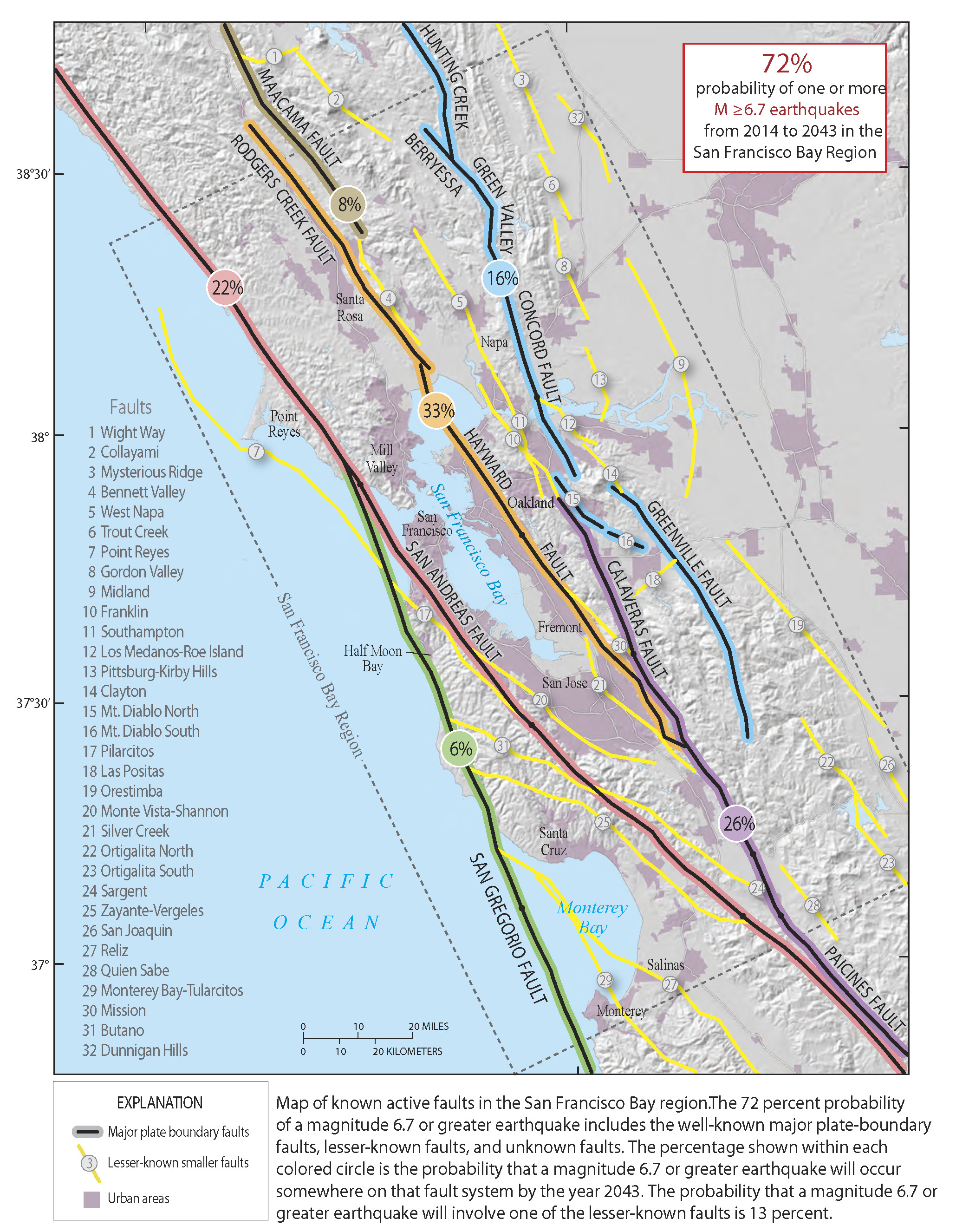
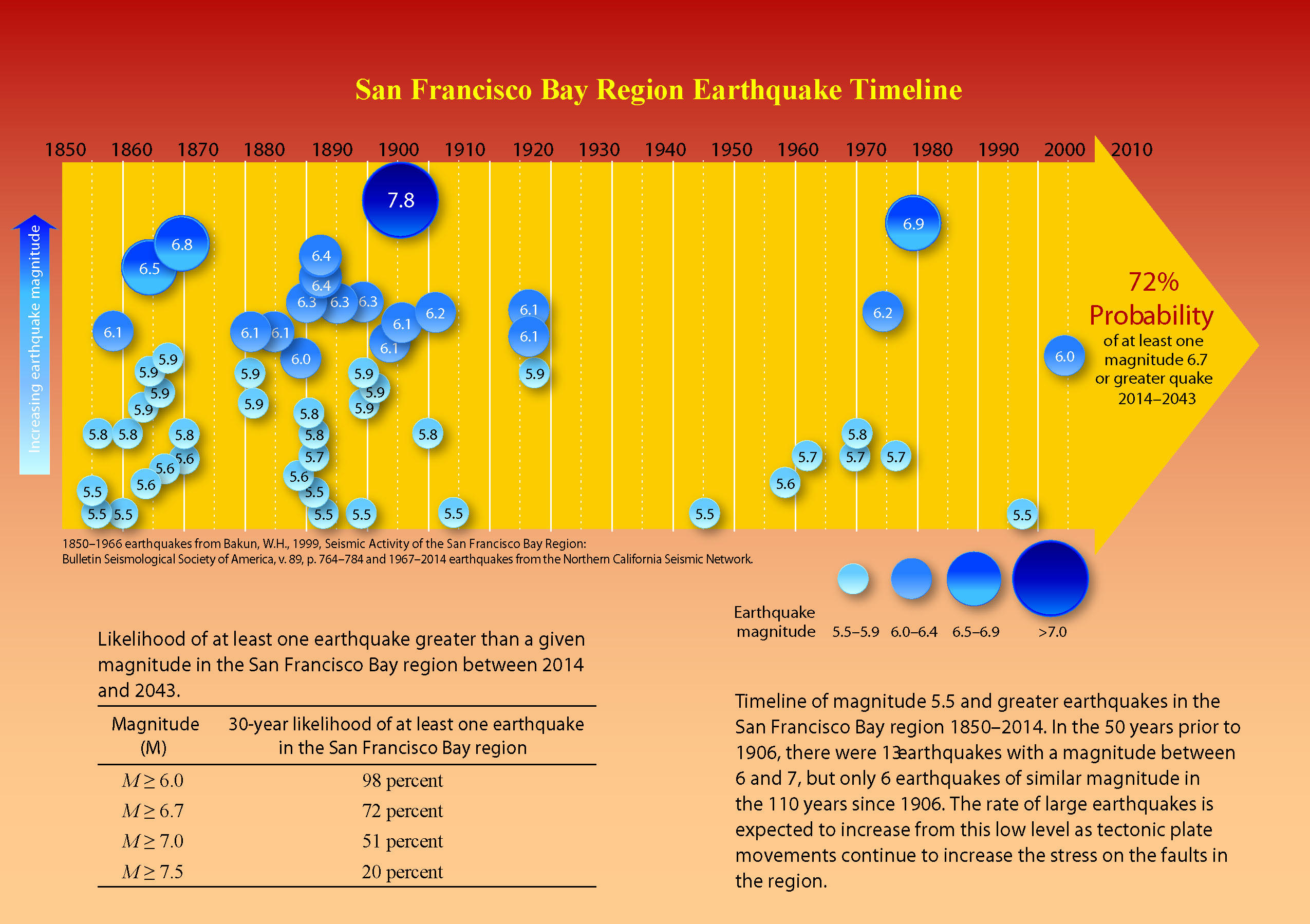
The cool part about the location of this earthquake is that it happened in a place that holds great interest to those in the seismic hazard community. In the SF Bay area, the Hayward – Rogers Creek fault system is the fault that has the highest probability of having an earthquake with a magnitude of M 6.7. There is a 33% chance that there will be a M ≥ 6.7 earthquake between 2014 and 2043.
Some have proposed that there is a step over, where these two faults overlap and there is some proportion of extension in this transfer zone. This hypothesis includes the idea that ruptures here may cause subsidence between the fault strands, causing a local tsunami in the area.
Others hypothesize that these faults are more directly linked. USGS geologists like Janet Watt have been conducting seismic reflection and sediment coring studies to evaluate this likelihood. Here is a review of their work in San Pablo Bay.

From the USGS: Why does it matter?

The longer the stretch of fault that breaks during an earthquake, the stronger the quake. When two faults are close to one another, the earthquake can jump from one to the other, making the rupture longer and the shaking stronger. When two faults are directly connected, it’s even easier for earthquake rupture to continue from one fault to the next.
A break along the combined length of the Hayward and Rodgers Creek faults could produce a major earthquake of magnitude 7.4. That earthquake would release more than five times the energy released by the 1989 magnitude 6.9 Loma Prieta earthquake, which caused about $6 billion in damage and killed 63 people.
To estimate the earthquake hazard posed by the Hayward and Rodgers Creek faults, scientists need to understand whether and how the faults connect. Previous work showed that the two faults approach each other closely beneath San Pablo Bay, but their exact relationship remained a mystery.

The USGS researchers found that the Hayward fault appears to connect directly to the Rodgers Creek fault.

From the USGS: Unexpected trajectory

“Where the faults enter San Pablo Bay, the Hayward from the south and the Rodgers Creek from the north, their orientations suggest that they’ll run parallel to one another, separated by a space, or ‘stepover,’ of about 5 kilometers [3 miles],” said Janet Watt, USGS research geophysicist and lead author of the study. “So when we went out to map, we thought we were going to map details of the stepover—like minor fractures that might enable an earthquake rupture to cross from one fault to the other.”
As the data accumulated, however, the researchers saw that the Hayward fault strand they were mapping bends slightly to the right as it traverses San Pablo Bay, heading toward the Rodgers Creek fault.
They realized that they might be looking at a fault bend. The distinction is important because fault bends affect earthquake hazards differently than stepovers. These differences include how likely a break on one fault will continue on to the next, how much slip (movement of rock on either side of the fault) will occur, and where ground shaking will be strongest.

Another cool thing about today’s earthquake is that this year marks the anniversary of the last major earthquake on the Hayward fault in 1868. The USGS, CGS, and other organizations and agencies are rolling out Haywired, an earthquake scenario designed to help people to learn to become more prepared and more resilient to earthquake hazards in the SF Bay area. More can be found out about Haywired here. There is more layperson speak material on the Hayward fault here.

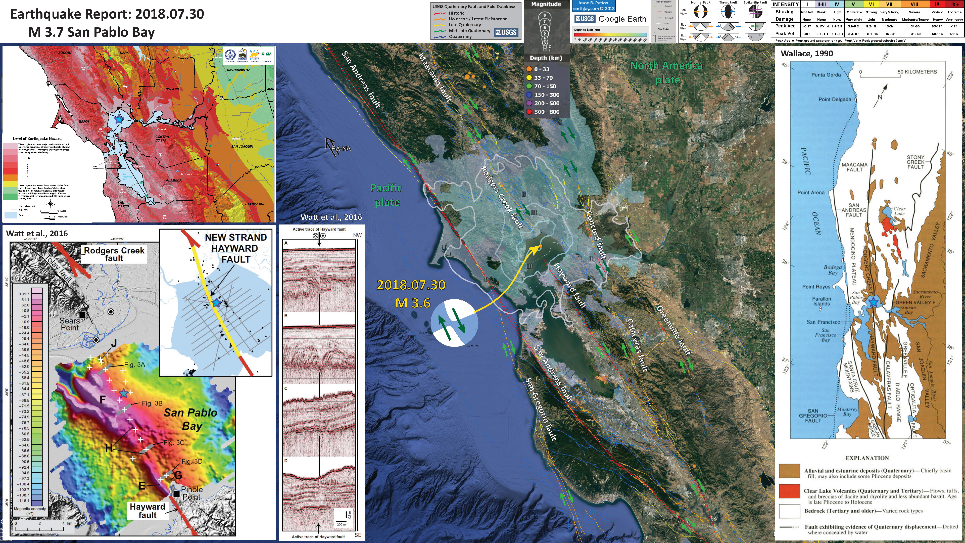
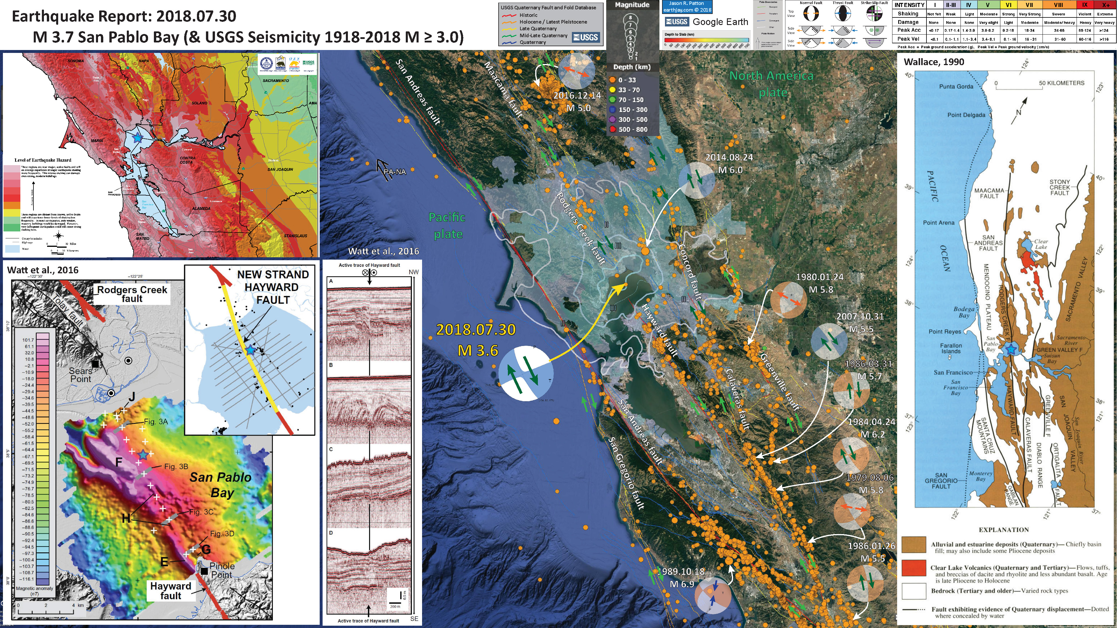
Below is my interpretive poster for this earthquake

I plot the seismicity from the past month, with color representing depth and diameter representing magnitude (see legend). I also include earthquake epicenters from 1918-2018 with magnitudes M ≥ 3.0 in one version of the poster.
I plot the USGS fault plane solutions (moment tensors in blue and focal mechanisms in orange), possibly in addition to some relevant historic earthquakes. Most earthquakes are strike-slip and aligned with the orientation of the plate boundary fault system. Some are normal (extensional) earthquakes which are probably places where faults are bending or stepping over. The 1989 event is the compressional Loma Prieta Earthquake. There is a good example of the earthquake types in the Geysers area (2016.12.14 M 5.0). These earthquakes often share this type of moment tensor, showing a poorly fit double couple (note how the corners of the beach ball are rounded, not sharp like the 1989 Loma Prieta focal mechanism. Most tectonic earthquakes are slip along a fault, which would ideally produce a double couple mechanism. When other types of seismic events occur (like volcanic explosions, nuclear test explosions, steam explosions, etc.) they have mechanisms that are not double couples.

I placed a moment tensor / focal mechanism legend on the poster. There is more material from the USGS web sites about moment tensors and focal mechanisms (the beach ball symbols). Both moment tensors and focal mechanisms are solutions to seismologic data that reveal two possible interpretations for fault orientation and sense of motion. One must use other information, like the regional tectonics, to interpret which of the two possibilities is more likely.
I also include the shaking intensity contours on the map. These use the Modified Mercalli Intensity Scale (MMI; see the legend on the map). This is based upon a computer model estimate of ground motions, different from the “Did You Feel It?” estimate of ground motions that is actually based on real observations. The MMI is a qualitative measure of shaking intensity. More on the MMI scale can be found here and here. This is based upon a computer model estimate of ground motions, different from the “Did You Feel It?” estimate of ground motions that is actually based on real observations.
I include the Did You Feel It?” felt reports data as a transparent overlay. The colors are based upon reports that people submit when they feel an earthquake. This is shown for a comparison between the modeled data (the MMI contours) and the DYFI data.

I include some inset figures.
On the right, I include generalized fault map of northern California from Wallace (1990). I place a blue star in the general location of today’s M 4.4 earthquake.
In the upper left corner is a map that shows the potential for shaking from earthquakes in central California, the San Francisco Bay area. This was published in 2003.
In the lower left corner is a figure from Watt et al. (2016). In the upper right is a map showing the blue San Pablo Bay. These authors collected subsurface data (seismic reflection, CHIRP) along lines shown in gray. In the main part of the map is a magnetic anomaly map, which shows how the magnetic field can be used to interrogate the structures and material types within the earth. This figure shows that the Hayward fault location can be inferred by the magnetic anomaly data. The gray bands labeled A, B, C, and D show the location of the seismic profiles shown on this poster.
To the right of the magnetic anomaly map is a series of 4 seismic profiles. The color changes (white to black) represent locations in the subsurface that have changes in material properties. These are most likely layers of sediment. Where layers are flat, the sediment may still be in place where it was deposited. Where the layers are folded, this may be evidence for tectonic deformation. Where these layers terminate along a line, this may show that there is an earthquake fault along that line. Note the observations you can make along the proposed location of the northern Hayward fault. I include this figure below so one may zoom in further.

Here is the interpretive poster with seismicity from the past month.

Here is the interpretive poster with seismicity from 1918-2018 for earthquakes M ≥ 3.0.

USGS Earthquake Pages

These are from this current sequence

2018-07-30 M 3.7 San Pablo Bay, CA

Some Relevant Discussion and Figures

Here is a fault map from Parsons et al., 2003. Note the configuration of the Hayward relative to the Rodgers Creek fault. These authors use seismic reflection and seismic tomography to interpret the subsurface in San Pablo Bay. The seismic profile below is located where the red line is shown on this map.

Fault map of San Pablo Bay based on the cross sections of Wright and Smith (1992) (cross section locations shown with black lines) and our new section in south San Pablo Bay (cross-section location shown with red line). We carry the Pinole fault offshore at least as far north as our cross section, and we connect the Rodgers Creek fault as far south as our section.

Here is the seismic profile (Parsons et al., 2003). Color represents material properties (seismic velocity). The black and white layers represent geologic materials with varying material properties (where there are layers of alternating material properties). These authors interpret faulting along this profile.

A structural cross section (upper 2 km) across south San Pablo Bay and the Hayward–Rodgers Creek step-over (see Fig. 1 for location). Seismic reflection data are overlain on a tomographic seismic velocity section. A significant lateral contrast is observed about 1 km east of the presently active trace of the Hayward fault and may represent an older fault trace. Another fault ~4 km east of the active Hayward fault separates east-dipping from west-dipping bedding within a basin; this structure is located on the Rodgers Creek fault trend projected from two structural sections in central and north San Pablo Bay developed by Wright and Smith (1992). Sparse relocated earthquake hypocenters (Waldhauser and Ellsworth, 2002) are shown in the lower panels with and without the Wright and Smith (1992) interpretation.

Here is their gravity map. Compare these results with the map from Watts et al. (2016; below and on the interpretive poster).

Gravity map of the San Pablo Bay region. An upward continued (500 m) signal was subtracted from the data, which filters out the broader wavelength features and allows us to focus on the shallowest part of the crust. A simplified fault map is shown by the black lines, and gravity gradients are identified by the white dots. A broad gravity low characterizes San Pablo Bay, and a subtly lower anomaly appears to coincide with the region between the Hayward and Rodgers Creek faults. This low is truncated near the north edge of San Pablo Bay by a strong gravity gradient that might be a normal fault boundary of a pull-apart basin.

This is the figure from Watts et al. (2016). I include their figure caption below.

Marine magnetic map of San Pablo Bay. Warm colors show magnetic highs, and cool colors show magnetic or dipole lows. Plus signs show locations of the offshore Hayward fault along chirp seismic profiles. Thick red lines show Late Pleistocene and younger traces of Hayward and Rodgers Creek faults (23). Black lines are older Quaternary faults (23). Thick gray lines show locations of seismic profiles in Fig. 3. Capital letters E, F, G, H, and J are discussed in the text. Black circles show exploratory well locations (5). Base map, 2010 (1m) National Oceanic and Atmospheric Administration Lidar. Inset: New Hayward fault strand (yellow) connecting directly to the Rodgers Creek fault. Gray lines show locations of chirp seismic track lines. Small black circles show relocated earthquakes (22).

Here are the 4 seismic profiles from Watt et al. (2016), their locations shown as gray bands in the above map. I include their figure caption below.

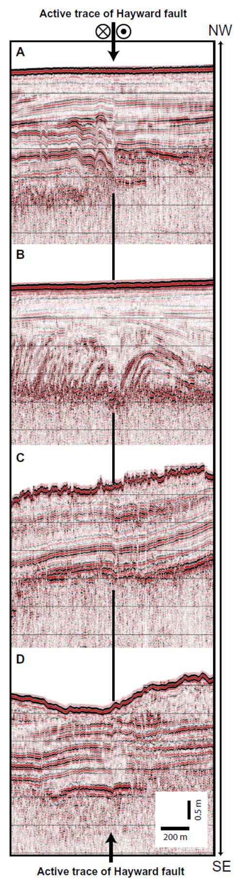
Chirp seismic profiles along the offshore Hayward fault. (A) to (D) are discussed in the text. Note vertical exaggeration of ~195:1. NW, northwest; SE, southeast.

Here is the isostatic gravity map from Watt et al. (2016). Gravity measurements have been modeled to account for the geometry of the earth (e.g. thickness of the crust or sections of the crust, sediment bodies, etc.), topography, etc. The result of this modeling can let us learn about structures like faults. I include their figure caption below.

Isostatic gravity map of San Pablo Bay. Map shows isostatic gravity anomalies in San Pablo Bay (45–47). Thick dashed white line shows the location of the horizontal gravity gradient maxima relative to the location of the Hayward fault (black plus signs). Orange star shows the location of a steep tomographic gradient along a seismic velocity profile (dotted black line) (6).

More about the background seismotectonics

I place a map shows the configuration of faults in central (San Francisco) and northern (Point Delgada – Punta Gorda) CA (Wallace, 1990). Here is the caption for this map, that is on the lower left corner of my map. Below the citation is this map presented on its own.

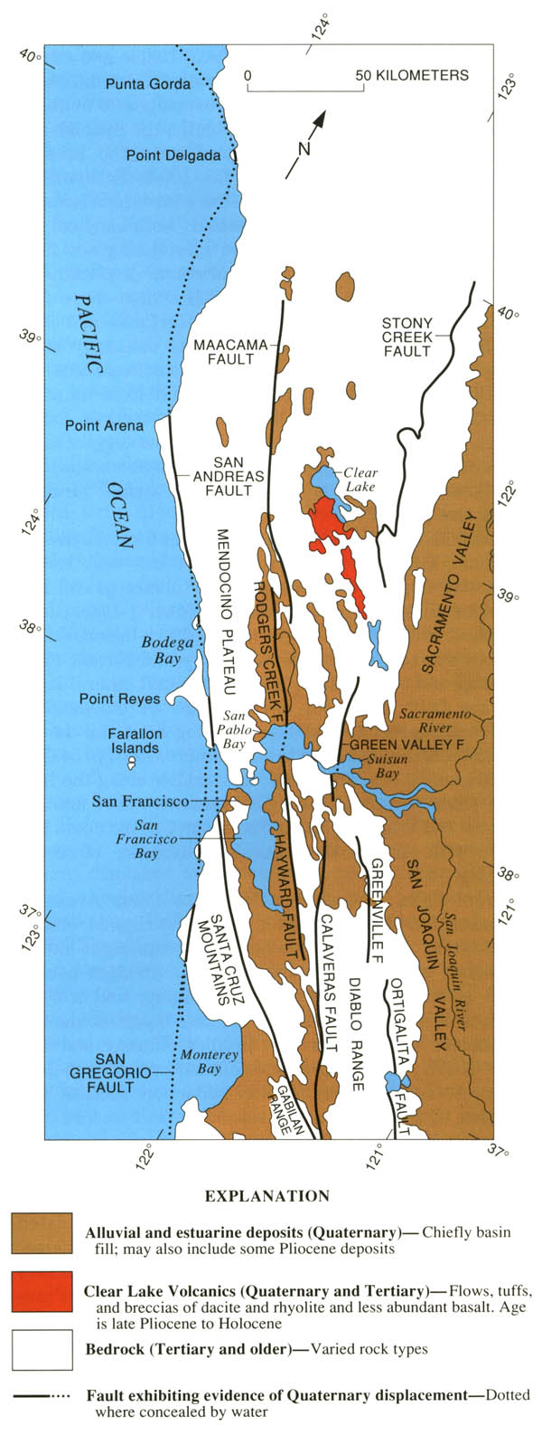
Geologic sketch map of the northern Coast Ranges, central California, showing faults with Quaternary activity and basin deposits in northern section of the San Andreas fault system. Fault patterns are generalized, and only major faults are shown. Several Quaternary basins are fault bounded and aligned parallel to strike-slip faults, a relation most apparent along the Hayward-Rodgers Creek-Maacama fault trend.

Here is the figure showing the evolution of the SAF since its inception about 29 Ma. I include the USGS figure caption below as a blockquote.

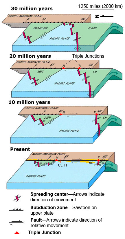
EVOLUTION OF THE SAN ANDREAS FAULT.
This series of block diagrams shows how the subduction zone along the west coast of North America transformed into the San Andreas Fault from 30 million years ago to the present. Starting at 30 million years ago, the westward- moving North American Plate began to override the spreading ridge between the Farallon Plate and the Pacific Plate. This action divided the Farallon Plate into two smaller plates, the northern Juan de Fuca Plate (JdFP) and the southern Cocos Plate (CP). By 20 million years ago, two triple junctions began to migrate north and south along the western margin of the West Coast. (Triple junctions are intersections between three tectonic plates; shown as red triangles in the diagrams.) The change in plate configuration as the North American Plate began to encounter the Pacific Plate resulted in the formation of the San Andreas Fault. The northern Mendicino Triple Junction (M) migrated through the San Francisco Bay region roughly 12 to 5 million years ago and is presently located off the coast of northern California, roughly midway between San Francisco (SF) and Seattle (S). The Mendicino Triple Junction represents the intersection of the North American, Pacific, and Juan de Fuca Plates. The southern Rivera Triple Junction (R) is presently located in the Pacific Ocean between Baja California (BC) and Manzanillo, Mexico (MZ). Evidence of the migration of the Mendicino Triple Junction northward through the San Francisco Bay region is preserved as a series of volcanic centers that grow progressively younger toward the north. Volcanic rocks in the Hollister region are roughly 12 million years old whereas the volcanic rocks in the Sonoma-Clear Lake region north of San Francisco Bay range from only few million to as little as 10,000 years old. Both of these volcanic areas and older volcanic rocks in the region are offset by the modern regional fault system. (Image modified after original illustration by Irwin, 1990 and Stoffer, 2006.)

Tectonic History of Western North America and Southern California

Here is an animation from Tanya Atwater that shows how the Pacific-North America plate margin evolved over the past 40 million years (Ma).

Here is a map from McLaughlin et al. (2012) that shows the regional faulting. I include the figure caption as a blockquote below.

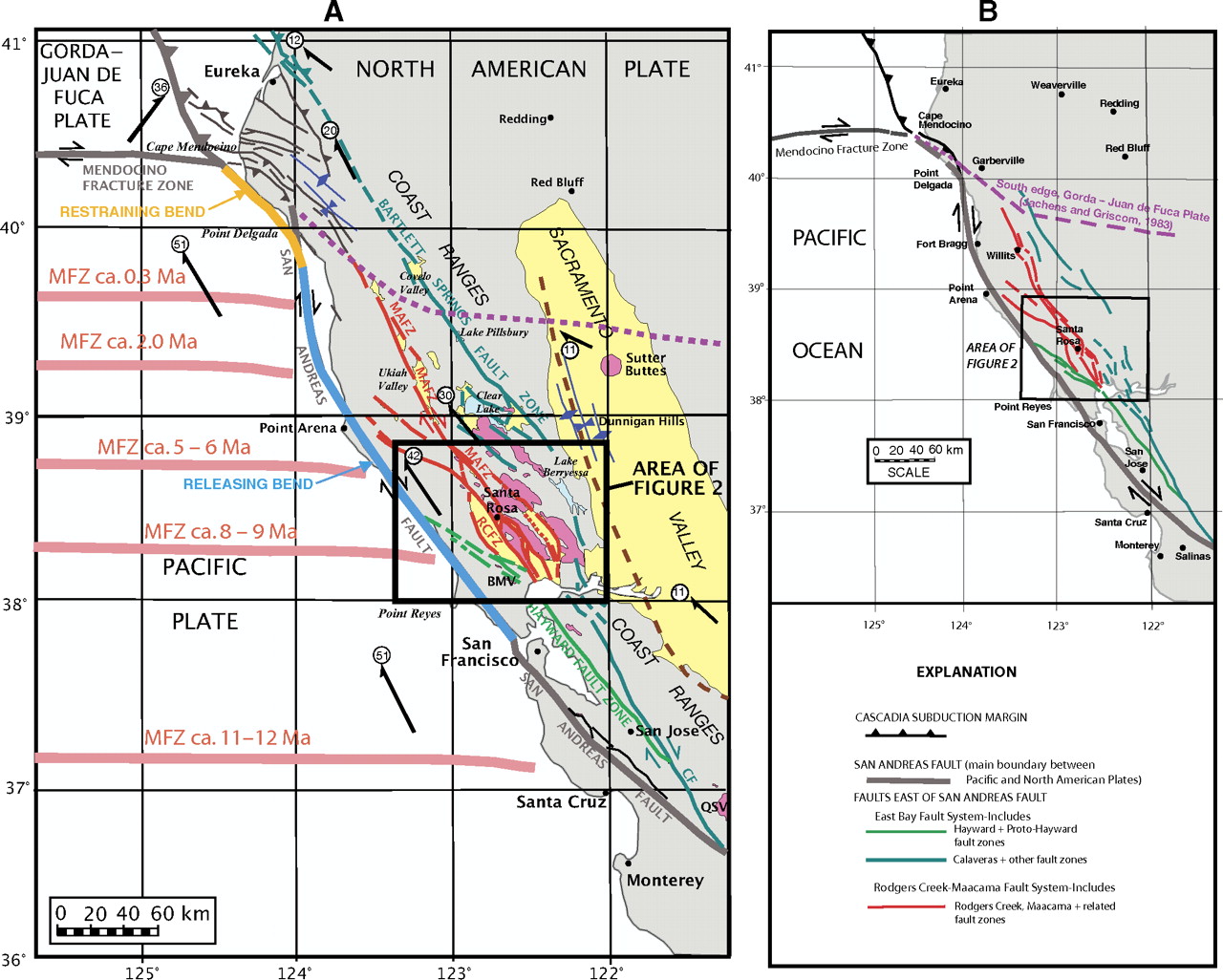
Maps showing the regional setting of the Rodgers Creek–Maacama fault system and the San Andreas fault in northern California. (A) The Maacama (MAFZ) and Rodgers Creek (RCFZ) fault zones and related faults (dark red) are compared to the San Andreas fault, former and present positions of the Mendocino Fracture Zone (MFZ; light red, offshore), and other structural features of northern California. Other faults east of the San Andreas fault that are part of the wide transform margin are collectively referred to as the East Bay fault system and include the Hayward and proto-Hayward fault zones (green) and the Calaveras (CF), Bartlett Springs, and several other faults (teal). Fold axes (dark blue) delineate features associated with compression along the northern and eastern sides of the Coast Ranges. Dashed brown line marks inferred location of the buried tip of an east-directed tectonic wedge system along the boundary between the Coast Ranges and Great Valley (Wentworth et al., 1984; Wentworth and Zoback, 1990). Dotted purple line shows the underthrust south edge of the Gorda–Juan de Fuca plate, based on gravity and aeromagnetic data (Jachens and Griscom, 1983). Late Cenozoic volcanic rocks are shown in pink; structural basins associated with strike-slip faulting and Sacramento Valley are shown in yellow. Motions of major fault blocks and plates relative to fi xed North America, from global positioning system and paleomagnetic studies (Argus and Gordon, 2001; Wells and Simpson, 2001; U.S. Geological Survey, 2010), shown with thick black arrows; circled numbers denote rate (in mm/yr). Restraining bend segment of the northern San Andreas fault is shown in orange; releasing bend segment is in light blue. Additional abbreviations: BMV—Burdell Mountain Volcanics; QSV—Quien Sabe Volcanics. (B) Simplifi ed map of color-coded faults in A, delineating the principal fault systems and zones referred to in this paper.

Here is a map that shows the shaking potential for earthquakes in CA. This comes from the state of California here.

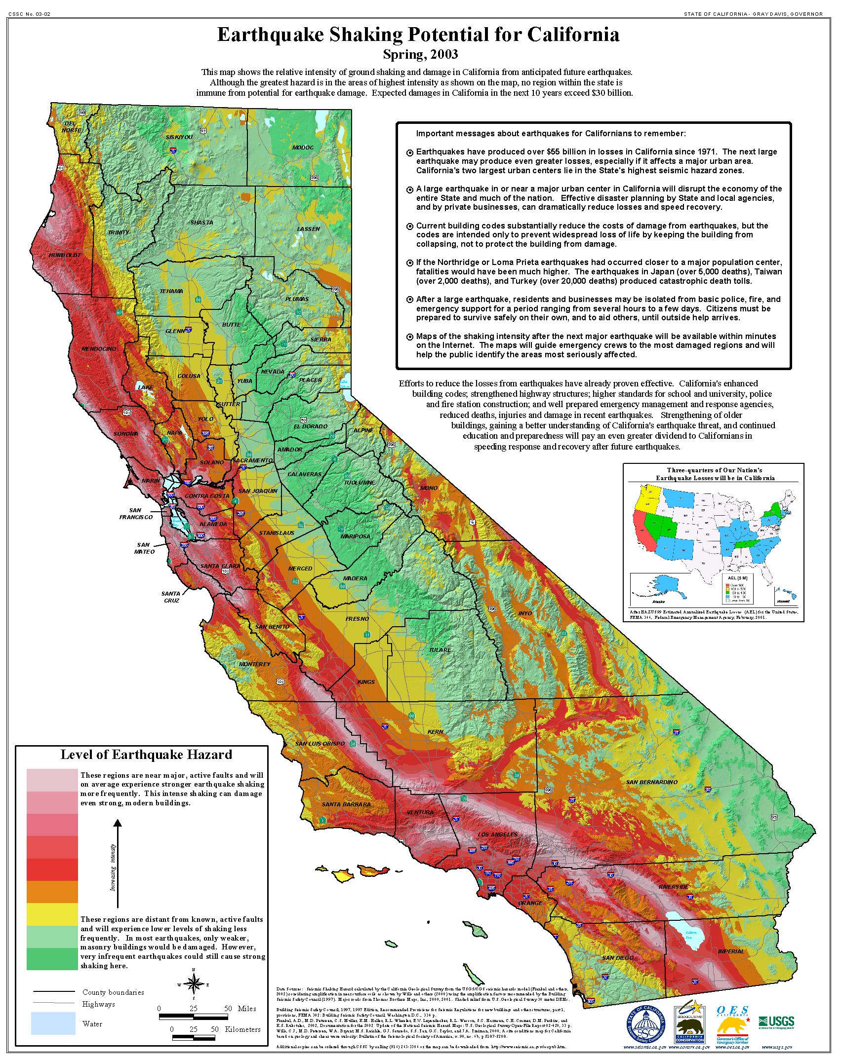
Earthquake shaking hazards are calculated by projecting earthquake rates based on earthquake history and fault slip rates, the same data used for calculating earthquake probabilities. New fault parameters have been developed for these calculations and are included in the report of the Working Group on California Earthquake Probabilities. Calculations of earthquake shaking hazard for California are part of a cooperative project between USGS and CGS, and are part of the National Seismic Hazard Maps. CGS Map Sheet 48 (revised 2008) shows potential seismic shaking based on National Seismic Hazard Map calculations plus amplification of seismic shaking due to the near surface soils.

Here is the earthquake probability map for the SF Bay area (Aagard et al., 2016).

This shows a timeline for historic earthquakes in this region (Aagaard et al., 2016).

Here is a map from the CGS that shows some of the detailed fault mapping done in this region. One can view this map on the CGS website here.

HayWired

There is much more about the Haywired scenario here.
However I include here a couple graphics to help us key into this knowledge of the past so we can prepare for the future.

Here is an estimate (from ground motion modeling) of the amount of shaking that might happen when the Hayward fault ruptures next (USGS, 2018). Remember that the Hayward fault is the fault in the SF Bay area that has the highest chance of going off in the next few decades. Red = severe shaking, green = moderate shaking.

This map of the San Francisco Bay region, California, shows simulated ground shaking caused by the hypothetical magnitude-7.0 mainshock of the HayWired earthquake scenario on the Hayward Fault. Red shows the most extreme ground shaking and where damage is the worst. The mainshock begins beneath the City of Oakland (star) and causes the Hayward Fault to rupture along about 52 miles of its length (thick black line). White lines are other major faults in the region.

Here is a map that shows what aftershocks and triggered earthquakes may happen as part of the result of the Hayward fault rupturing (USGS, 2018).

This map of California’s San Francisco Bay region shows the hypothetical mainshock and aftershock sequence of the HayWired earthquake scenario on the Hayward Fault. In the scenario, aftershocks are modeled for 2 years after the mainshock—an innovation unique to HayWired. Early in the sequence, most aftershocks are concentrated near the Hayward Fault.

Informational Video: HayWired

Geologic Fundamentals

For more on the graphical representation of moment tensors and focal mechnisms, check this IRIS video out:

Here is a fantastic infographic from Frisch et al. (2011). This figure shows some examples of earthquakes in different plate tectonic settings, and what their fault plane solutions are. There is a cross section showing these focal mechanisms for a thrust or reverse earthquake. The upper right corner includes my favorite figure of all time. This shows the first motion (up or down) for each of the four quadrants. This figure also shows how the amplitude of the seismic waves are greatest (generally) in the middle of the quadrant and decrease to zero at the nodal planes (the boundary of each quadrant).

There are three types of earthquakes, strike-slip, compressional (reverse or thrust, depending upon the dip of the fault), and extensional (normal). Here is are some animations of these three types of earthquake faults. The following three animations are from IRIS.

Strike Slip:

Compressional:

Extensional:

This is an image from the USGS that shows how, when an oceanic plate moves over a hotspot, the volcanoes formed over the hotspot form a series of volcanoes that increase in age in the direction of plate motion. The presumption is that the hotspot is stable and stays in one location. Torsvik et al. (2017) use various methods to evaluate why this is a false presumption for the Hawaii Hotspot.

A cutaway view along the Hawaiian island chain showing the inferred mantle plume that has fed the Hawaiian hot spot on the overriding Pacific Plate. The geologic ages of the oldest volcano on each island (Ma = millions of years ago) are progressively older to the northwest, consistent with the hot spot model for the origin of the Hawaiian Ridge-Emperor Seamount Chain. (Modified from image of Joel E. Robinson, USGS, in “This Dynamic Planet” map of Simkin and others, 2006.)

Here is a map from Torsvik et al. (2017) that shows the age of volcanic rocks at different locations along the Hawaii-Emperor Seamount Chain.

Hawaiian-Emperor Chain. White dots are the locations of radiometrically dated seamounts, atolls and islands, based on compilations of Doubrovine et al. and O’Connor et al. Features encircled with larger white circles are discussed in the text and Fig. 2. Marine gravity anomaly map is from Sandwell and Smith.

San Andreas fault Earthquake Reports

General Overview