The other evening (my time) I and many others noticed a series of earthquakes in the Banda Sea region.
As is typical, people want as much information about these earthquakes as possible as soon as possible.
There were two quakes within about a minute of each other (first M 6.7, then M 7.1), so it was possible that there was actually just one earthquake (or so we thought).
The reason for this is that sometimes the automated earthquake location algorithms get it wrong. That is when real people step in to review the data from the available seismic networks (data from seismometers that measure seismic waves from earthquakes).
Long story short, these two earthquakes were actually different earthquakes. After a while, the magnitudes stopped changing. And, a while later, another M 6.7 earthquake happened.
- 2023-11-08 04:52:51 (UTC) M 6.7: https://earthquake.usgs.gov/earthquakes/eventpage/us7000l9h2/executive
- 2023-11-08 04:53:50 (UTC) M 7.1: https://earthquake.usgs.gov/earthquakes/eventpage/us7000l9h4/executive
- 2023-11-08 13:02:06 (UTC) M 6.7: https://earthquake.usgs.gov/earthquakes/eventpage/us7000l9ku/executive
Here are the these three earthquakes:
In this part of the world, there are several different plate boundary faults that interact.
To the south of the Banda Sea, there is a subduction zone. This is a convergent plate boundary fault where an oceanic plate (Australia plate) “subducts” beneath the Sunda plate (part of the Eurasia plate).
This subduction zone extends laterally from between Australia and the Timor Islands, westward through Java and Sumatra, up to Myanmar/Burma. This plate boundary is part of the Alpide Belt, a convergent plate boundary that spans this region, all the way westward past Portugal and Morroco!
There are also some strike-slip faults in the upper plate here. These may be related to faults that extend further to the east, heading into Papua New Guinea and the “Bird’s Head.” One of these faults is the Sorong fault.
When I first saw this earthquake, I thought about the previous Earthquake Reports I had developed for events in this region. Every one of them were for intermediate depth earthquakes within the subducted Australia plate.
The mechanism for this M 7.1 was strike-slip and matched many of the mechanisms from these earlier earthquakes. However, the depth was set at 10 km. This is one of the default earthquake depths, so I thought that it might be updated later to be much deeper. Though, when earthquakes are so much deeper, their initial depths are often not set at the default 10 km depth.
So, I posted to social media that this may be one of these intermediate depth intraslab (within the slab of the plate) earthquakes. I suggested that the depth may be updated, as I mention here ^^^.
Well, it is always good to be receptive to one being incorrect. I was incorrect. That is OK! In the early hours (even days) after an earthquake, everyone is trying to figure out what happened. I don’t want to hold back my imagination from conceiving of hypotheses. But, I do want to be open minded that I need to change my interpretations given more information as that rolls in.
One of these pieces of information was data from a nearby tide gage, a gage located on the Island of Damar (less than 100 km from the epicenter). This tide gage showed a tsunami being recorded.
Strike-slip earthquakes are generally thought to not generate tsunami. Though, the 1906 San Francisco, the 1999 Izmit, and the 2018 Dongalla-Palu earthquakes did. Generally they are simply smaller in size (Dongalla-Palu being an exception, given the configuration of Palu Bay).
If the moderate sized strike-slip earthquake were intermediate depth, it is extremely unlikely to generate a tsunami as there would be very little deformation of the seafloor. Because this M 7.1 generated a tsunami, it supported the shallow depths and a crustal source for this earthquake.
So, this series of earthquakes was indeed shallower, within the upper plate (not the Australia plate). AND there is this strike-slip fault that is already mapped, probably the source for these earthquakes.
A second thing about the tide gage plots is that we can see that the second M 6.7 earthquake also generated a tsunami! Much smaller, but a signal that can be found on several tide gage records.
Indonesia operates an extensive tide gage network. Here one can locate all the gages in their network.
Below I present an interpretive poster and some supporting material.
Below is my interpretive poster for this earthquake
- I plot the seismicity from the past month, with diameter representing magnitude (see legend). I include earthquake epicenters from 1923-2023 with magnitudes M ≥ 7.0 in one version.
- I plot the USGS fault plane solutions (moment tensors in blue and focal mechanisms in orange), possibly in addition to some relevant historic earthquakes.
- A review of the basic base map variations and data that I use for the interpretive posters can be found on the Earthquake Reports page. I have improved these posters over time and some of this background information applies to the older posters.
- Some basic fundamentals of earthquake geology and plate tectonics can be found on the Earthquake Plate Tectonic Fundamentals page.
- In the upper right corner is a map showing plate boundary fault lines and the major tectonic plates.
- To the left of the plate tectonic map is an inset, larger scale map, showing the aftershocks from a couple days. I outline what may be the main fault rupture area, plus a secondary rupture for triggered earthquakes. Based on Wells and Coppersmith (1994), the aftershocks span a region larger in size than expected for a 7.1. So, there may be several faults involved here. Perhaps the second M 6.7 was also a triggered earthquake (on a different fault), not an aftershock(?).
- In the center right is a low angle oblique view of the tectonic plate configuration (Pownall et al., 2014). The previous earthquakes in the poster that have mechanisms plotted all appear to be in the subducted Australia plate, shown here diving downwards.
- In the lower right corner is a view of the tectonic plate configuration (Koulali et al., 2014). I place a blue star in the location of the M 7.1 earthquake. Note that there is an earthquake from 1763 with a magnitude 7 located along the strike-slip fault mapped on this map. This earthquake generated a tsunami.
- In the upper left corner are maps that show the seismic hazard and seismic risk for Indonesia. I spend more time explaining this below.
- In the center top-left is a map that shows earthquake intensity using the Modified Mercalli Intensity (MMI) Scale.
- In the bottom center I plot the tide gage data from Damar Island.
I include some inset figures. Some of the same figures are located in different places on the larger scale map below.
- Here is the map with a month’s seismicity plotted.
Tsunami Hazard
- Here are two maps that show the results of probabilistic tsunami modeling for the nation of Indonesia (Horspool et al., 2014). These results are similar to results from seismic hazards analysis and maps. The color represents the chance that a given area will experience a certain size tsunami (or larger).
- The first map shows the annual chance of a tsunami with a height of at least 0.5 m (1.5 feet). The second map shows the chance that there will be a tsunami at least 3 meters (10 feet) high at the coast.
- Here are two tide gage records that include observations from the M 7.1 and M 6.7 earthquakes. There were a couple other gages in the region that include the tsunami but the tsunami was very small and difficult to accurately measure.
Annual probability of experiencing a tsunami with a height at the coast of (a) 0.5m (a tsunami warning) and (b) 3m (a major tsunami warning).
- Here is a tectonic map for this part of the world from Zahirovic et al., 2014. They show a fracture zone where the M 7.3 earthquake happened. I left out all the acronym definitions (you’re welcome), but they are listed in the paper.
- Here are a series of maps from Koulali et al. (2014).
- This first one shows the major historic earthquakes at the time of publication (also, this is the map in the interpretive poster).
- This map shows the plate velocities as measured by GPS/GNSS instruments.
- Note the blue arrows show the convergent nature of the plate boundary to the south of this earthquake.
- This map shows the results of their plate tectonic modeling.
- Koulali et al. (2014) basically modeled the different tectonic blocks and made estimates of how much each plate boundary fault would need to move based on these block motions.
- Here we can see that there is lateral motion required for the strike-slip fault that may be the causative fault for this M 7.1 earthquake sequence.
- This is a great visualization showing the Australia plate and how it formed the largest forearc basin on Earth (Pownall et al., 2014).
- The maps on the left show a time history of the tectonics. The low angle oblique view on the right shows the dipping crust (north is not always up, as in this figure).
- In the lower right, they show how there is strike-slip faulting along the Seram trough also (I left out the figure caption for E).
- Here is a map and some cross sections showing seismic tomography (like C-T scans into the Earth using seismic waves instead of X-Rays). The map shows the location of the cross sections (Spakman et al., 2010).
- Here is the map from Benz et al. (2011).
- Here is the tectonic map from Hengesh and Whitney (2016)
- Here is the Audley (2011) cross section showing how the backthrust relates to the subduction zone beneath Timor. I include their figure caption in blockquote below.
- Here is a figure showing the regional geodetic motions (Bock et al., 2003). I include their figure caption below as a blockquote.
- Whitney and Hengesh (2015) used GPS modeling to suggest a model of plate blocks. Below are their model results.
- Here is the conceptual model from Whitney and Hengesh (2015) that shows how left-lateral strike-slip faulting can come into the region.
Some Relevant Discussion and Figures

Regional tectonic setting with plate boundaries (MORs/transforms = black, subduction zones = teethed red) from Bird (2003) and ophiolite belts representing sutures modified from Hutchison (1975) and Baldwin et al. (2012). West Sulawesi basalts are from Polvé et al. (1997), fracture zones are from Matthews et al. (2011) and basin outlines are from Hearn et al. (2003).
Seismotectonic setting of the Sunda-Banda arc-continent collision, East Indonesia. Major faults (thick black lines) [Hamilton, 1979]. Topography and bathymetry are from Shuttle Radar Topography Mission (http://topex.ucsd.edu/www_html/srtm30_plus.html). Focal mechanisms are from the Global Centroid Moment Tensor. Blue mechanisms correspond to earthquakes with Mw>7 (brown transparent ellipses are the corresponding rupture areas for Flores 1992 and Alor 2004 earthquakes), while the green focal mechanism shows the highest magnitude recorded in Sumbawa. Red dots indicate the locations of major historical earthquakes [Musson, 2012].
GPS velocities determined in this study with respect to Sunda Block. Uncertainty ellipses represent 95% confidence level. The inset figure corresponds to the area of the dashed rectangle in the map. Light blue arrows show the velocities for East and West Makassar Blocks.
Relative slip vectors across block boundaries, derived from our best fit model. Arrows show motion of the hanging wall (moving block) relative to the footwall (fixed block) with 95% confidence ellipses. The tails of arrows is located within the “moving” block. Black thick lines show well-defined boundaries we use as active faults in our model and dashed lines show less well-defined boundaries (green : free-slipping boundaries and black: fixed locked faults). Principal axes of the horizontal strain tensor estimated for the SUMB, EMAK, and EJAV are shown in pink. The thick pink arrow shows the relative motion of Australia with respect to Sunda (AUST/SUND). Abbreviations are Sumba Block (SUMB), West Makassar Block (WMAK), East Makassar Block (EMAK), East Java Block (EJAV), and Timor Block (TIMO). The background seismicity is from the International Seismological Centre catalog with magnitudes ≥5.5 and depths <40 km.

Reconstructions of eastern Indonesia, adapted from Hall (2012), depict collision of Australia with Southeast Asia and slab rollback into Banda Embayment. Yellow star indicates Seram. Oceanic crust is shown in purple (older than 120 Ma) and blue (younger than 120 Ma); submarine arcs and oceanic plateaus are shown in cyan; volcanic island arcs, ophiolites, and material accreted along plate margins are shown in green. A: Reconstruction at 15 Ma. B: Reconstruction at 7 Ma. C: Reconstruction at 2 Ma. D: Visualization of present-day slab morphology of proto–Banda Sea based on earthquake hypocenter distribution and tomographic models

The Banda arc and surrounding region. 200 m and 4,000 m bathymetric contours are indicated. The numbered black lines are Benioff zone contours in kilometres. The red triangles are Holocene volcanoes (http://www.volcano.si.edu/world/). Ar=Aru, Ar Tr=Aru trough, Ba=Banggai Islands, Bu=Buru, SBS=South Banda Sea, Se=Seram, Sm=Sumba, Su=Sula Islands, Ta=Tanimbar, Ta Tr=Tanimbar trough, Ti=Timor, W=Weber Deep.

Tomographic images of the Banda slab. Vertical sections through the tomography model along the lines shown in Fig. 1. Colours: P-wave anomalies with reference to velocity model ak135 (ref. 30). Dots: earthquake hypocentres within 12 km of the section. The dashed lines are phase changes at ~410 km and ~660 km. The sections are plotted without vertical exaggeration; the horizontal axis is in degrees. The labelled positive anomalies are the Sunda (Su) and Banda (Ba) slabs: BuDdetached slab under Buru, FlDslab under Flores, SDslab under Seram, TDslab under Timor. a, The Sunda slab enters the lower mantle whereas the Banda embayment slab is entirely in the upper mantle with the change under Sulawesi. b–e, Banda slab morphology in sections parallel to Australia plate motion shows a transition from a steep slab with a flat section (fs) (b) to a spoon shape shallowing eastward (c–e).


Illustration of major tectonic elements in triple junction geometry: tectonic features labeled per Figure 1; seismicity from ISC-GEM catalog [Storchak et al., 2013]; faults in Savu basin from Rigg and Hall [2011] and Harris et al. [2009]. Purple line is edge of Australian continental basement and fore arc [Rigg and Hall, 2011]. Abbreviations: AR = Ashmore Reef; SR = Scott Reef; RS = Rowley Shoals; TCZ = Timor Collision Zone; ST = Savu thrust; SB = Savu Basin; TT = Timor thrust; WT =Wetar thrust; WASZ = Western Australia Shear Zone. Open arrows indicate relative direction of motion; solid arrows direction of vergence.

Cartoon cross section of Timor today, (cf. Richardson & Blundell 1996, their BIRPS figs 3b, 4b & 7; and their fig. 6 gravity model 2 after Woodside et al. 1989; and Snyder et al. 1996 their fig. 6a). Dimensions of the filled 40 km deep present-day Timor Tectonic Collision Zone are based on BIRPS seismic, earthquake seismicity and gravity data all re-interpreted here from Richardson & Blundell (1996) and from Snyder et al. (1996). NB. The Bobonaro Melange, its broken formation and other facies are not indicated, but they are included with the Gondwana mega-sequence. Note defunct Banda Trench, now the Timor TCZ, filled with Australian continental crust and Asian nappes that occupy all space between Wetar Suture and the 2–3 km deep deformation front north of the axis of the Timor Trough. Note the much younger decollement D5 used exactly the same part of the Jurassic lithology of the Gondwana mega-sequence in the older D1 decollement that produced what appears to be much stronger deformation.

Topographic and tectonic map of the Indonesian archipelago and surrounding region. Labeled, shaded arrows show motion (NUVEL-1A model) of the first-named tectonic plate relative to the second. Solid arrows are velocity vectors derived from GPS surveys from 1991 through 2001, in ITRF2000. For clarity, only a few of the vectors for Sumatra are included. The detailed velocity field for Sumatra is shown in Figure 5. Velocity vector ellipses indicate 2-D 95% confidence levels based on the formal (white noise only) uncertainty estimates. NGT, New Guinea Trench; NST, North Sulawesi Trench; SF, Sumatran Fault; TAF, Tarera-Aiduna Fault. Bathymetry [Smith and Sandwell, 1997] in this and all subsequent figures contoured at 2 km intervals.

Plate boundary segments in the Banda Arc region from Nugroho et al (2009). Numbers inside rectangles show possible micro-plate blocks near the Sumba Triple Junction (colored) based on GPS velocities (black arrows) with in a stable Eurasian reference frame.
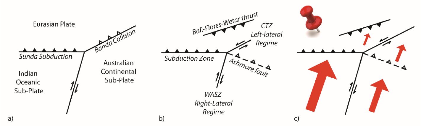
Schematic map views of kinematic relations between major crustal elements in the Sumba Triple Junction region. CTZ= collisional tectonic zone. Red arrow size designates schematic plate motion relations based on geological data relative to a fixed Sunda shelf reference frame (pin).
Seismic Hazard and Seismic Risk
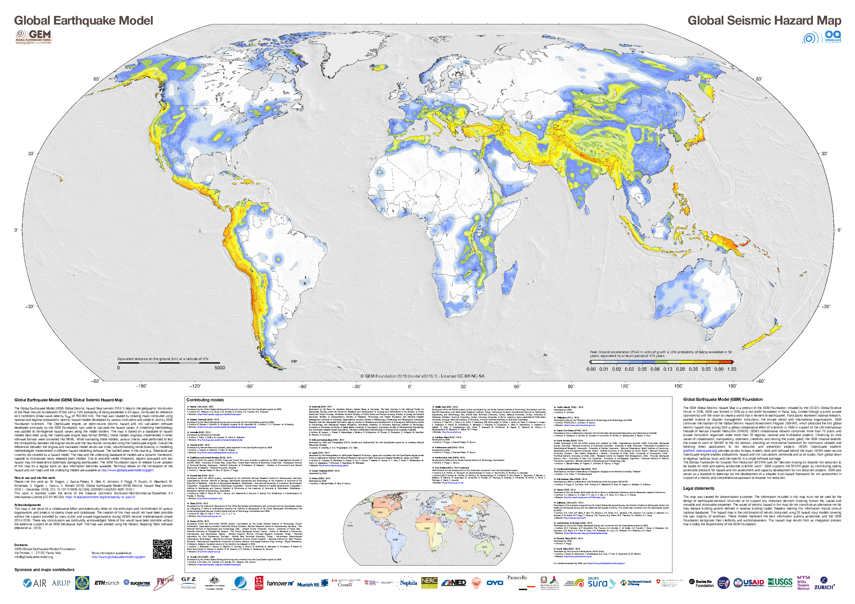
- These are the two maps shown in the map above, the GEM Seismic Hazard and the GEM Seismic Risk maps from Pagani et al. (2018) and Silva et al. (2018).
- The GEM Seismic Hazard Map:
- The Global Earthquake Model (GEM) Global Seismic Hazard Map (version 2018.1) depicts the geographic distribution of the Peak Ground Acceleration (PGA) with a 10% probability of being exceeded in 50 years, computed for reference rock conditions (shear wave velocity, VS30, of 760-800 m/s). The map was created by collating maps computed using national and regional probabilistic seismic hazard models developed by various institutions and projects, and by GEM Foundation scientists. The OpenQuake engine, an open-source seismic hazard and risk calculation software developed principally by the GEM Foundation, was used to calculate the hazard values. A smoothing methodology was applied to homogenise hazard values along the model borders. The map is based on a database of hazard models described using the OpenQuake engine data format (NRML). Due to possible model limitations, regions portrayed with low hazard may still experience potentially damaging earthquakes.
- Here is a view of the GEM seismic hazard map for Indonesia.
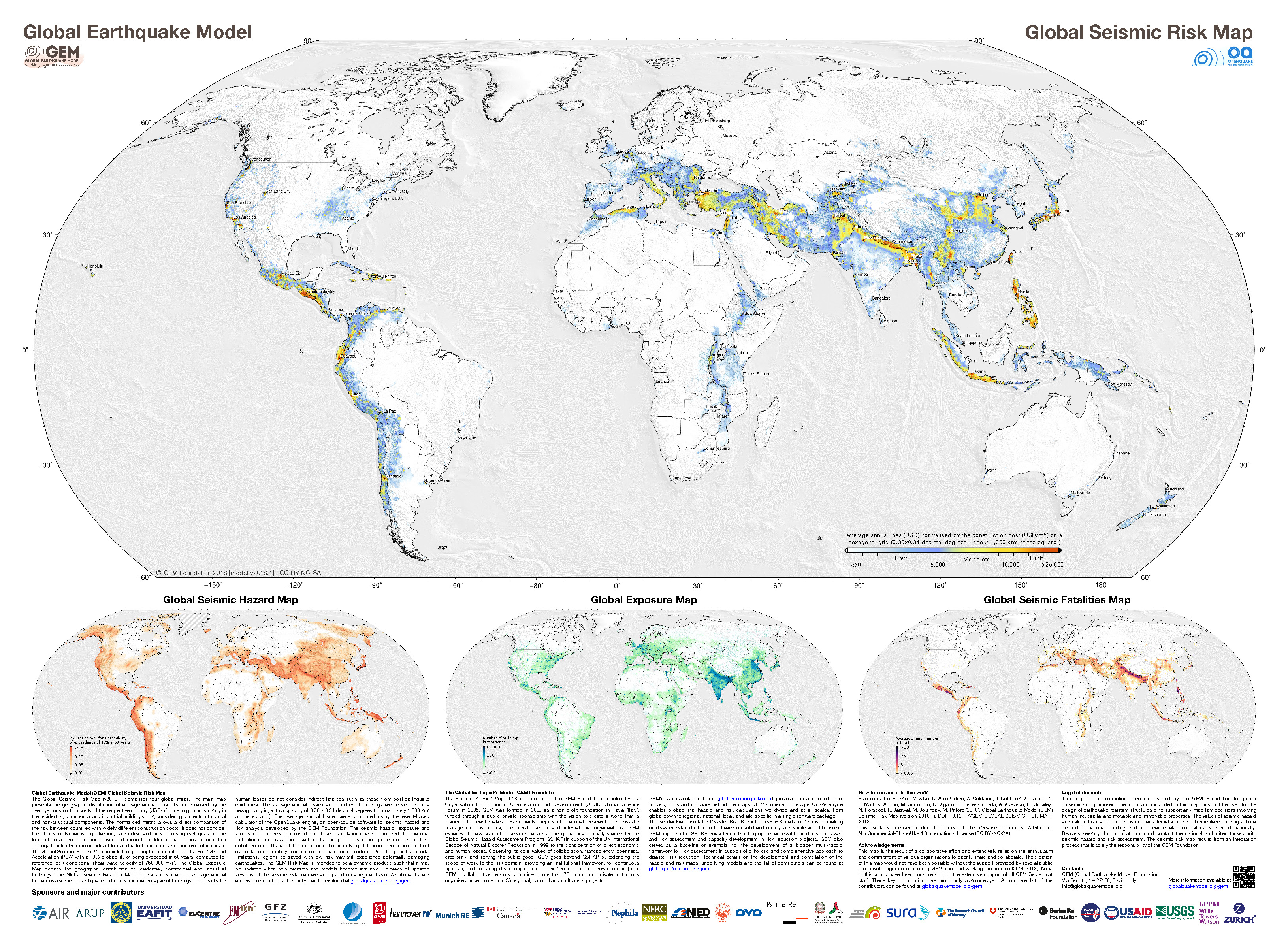
- The GEM Seismic Risk Map:
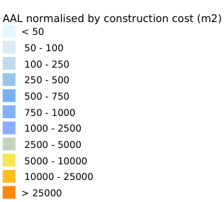
- The Global Seismic Risk Map (v2018.1) presents the geographic distribution of average annual loss (USD) normalised by the average construction costs of the respective country (USD/m2) due to ground shaking in the residential, commercial and industrial building stock, considering contents, structural and non-structural components. The normalised metric allows a direct comparison of the risk between countries with widely different construction costs. It does not consider the effects of tsunamis, liquefaction, landslides, and fires following earthquakes. The loss estimates are from direct physical damage to buildings due to shaking, and thus damage to infrastructure or indirect losses due to business interruption are not included. The average annual losses are presented on a hexagonal grid, with a spacing of 0.30 x 0.34 decimal degrees (approximately 1,000 km2 at the equator). The average annual losses were computed using the event-based calculator of the OpenQuake engine, an open-source software for seismic hazard and risk analysis developed by the GEM Foundation. The seismic hazard, exposure and vulnerability models employed in these calculations were provided by national institutions, or developed within the scope of regional programs or bilateral collaborations.
- Here is a view of the GEM seismic risk map for Indonesia.


- M 9.2 Andaman-Sumatra subduction zone 2014 Earthquake Anniversary
- M 9.2 Andaman-Sumatra subduction zone SASZ Fault Deformation
- M 9.2 Andaman-Sumatra subduction zone 2016 Earthquake Anniversary
- 2023.11.08 M 7.1 Banda Sea
- 2023.08.28 M 7.1 Lombok & Bali, Indonesia
- 2023.04.24 M 7.1 Sumatra
- 2022.11.18 M 6.9 Sumatra
- 2022.02.25 M 6.2 Sumatra
- 2020.05.06 M 6.8 Banda Sea
- 2019.08.02 M 6.9 Indonesia
- 2019.06.23 M 7.3 Banda Sea
- 2019.04.12 M 6.8 Sulawesi, Indonesia
- 2018.09.28 M 7.5 Sulawesi
- 2018.10.16 M 7.5 Sulawesi UPDATE #1
- 2018.08.19 M 6.9 Lombok, Indonesia
- 2018.08.05 M 6.9 Lombok, Indonesia
- 2018.07.28 M 6.4 Lombok, Indonesia
- 2017.12.15 M 6.5 Java
- 2017.08.31 M 6.3 Mentawai, Sumatra
- 2017.08.13 M 6.4 Bengkulu, Sumatra, Indonesia
- 2017.05.29 M 6.8 Sulawesi, Indonesia
- 2017.03.14 M 6.0 Sumatra
- 2017.03.01 M 5.5 Banda Sea
- 2016.10.19 M 6.6 Java
- 2016.03.02 M 7.8 Sumatra/Indian Ocean
- 2015.07.22 M 5.8 Andaman Sea
- 2015.11.08 M 6.4 Nicobar Isles
- 2012.04.11 M 8.6 Sumatra outer rise
- 2004.12.26 M 9.2 Andaman-Sumatra subduction zone
Indonesia | Sumatra
General Overview
Earthquake Reports
Social Media
Here is my main thread, which includes many intermediate tweets (one can see the process of us figuring this sequence out in real time):
#EarthquakeReport for M6.9 #Gempa #Earthquake offshore in the #BandaSea
Probably intraslab earthquake within Australia plate
In almost same location as 2020 earthquake: https://t.co/DBTKHT6oYnhttps://t.co/yE3fOxqZoO pic.twitter.com/nNAIGl7EaL
— Jason "Jay" R. Patton (@patton_cascadia) November 8, 2023
#EarthquakeReport #TsunamiReport for M 7.1 #Gempa #Earthquake sequence in the #BandaSea
M6.7 foreshock to 7.1 both left-lateral strike-slip earthquakes in the Sunda block crust
triggered a M 6.7
both the 7.1 and triggered 6.7 caused tsunamiread reporthttps://t.co/V9Y1zX4sRr pic.twitter.com/MEot8TVrlU
— Jason "Jay" R. Patton (@patton_cascadia) November 10, 2023
Mw=7.5, BANDA SEA (Depth: 16 km), 2023/11/08 04:52:52 UTC – Full details here: https://t.co/UPXunwhyVI pic.twitter.com/fPFfoh3zUu
— Earthquakes (@geoscope_ipgp) November 8, 2023
This seismic signal actually shows two earthquakes in approx. the same location in the Banda Sea, ~1 min apart – the first a M7.0, the second a M7.1. Our recorders were still picking up a signal >30 mins later. https://t.co/TLOo9ts3yM pic.twitter.com/ztEZGUEECx
— Dr. Dee Ninis (@DeeNinis) November 8, 2023
data monitoring paras muka air laut di stasiun pengamamatan Damar Maluku 12:53 WIB 08/11/2023 cc: @widjokongko pic.twitter.com/oXIklbZtsG
— INFOMITIGASI (@infomitigasi) November 8, 2023
Rabu 08 Nov 2023 pukul 11.52.53 WIB Laut Banda diguncang gempa tektonik. Hasil analisis BMKG menunjukkan gempa ini memiliki parameter update M7,1. Episenter gempa terletak di laut pada jarak 255 Km arah Barat Laut Tanimbar, Maluku pada kedalaman 45 km. pic.twitter.com/AgO1mx94Ka
— DARYONO BMKG (@DaryonoBMKG) November 8, 2023
Today, 7.2 Eq. Banda Sea (Eastern #INDONESIA 🇮🇩), located in the "Inner Banda Arc" (close to Extinct Damar Spreading Basin), crustal strike-slip faulting suggest reactivation of "Damar Extinct Spreading Back-arc Basin (NW-SE structure?).
🔹️Damar Basin :https://t.co/7mSB8NnO4R pic.twitter.com/ZZF6AVeC6n
— Abel Seism🌏Sánchez (@EQuake_Analysis) November 8, 2023
Watch the earthquake waves from these events in Indonesia sweep across North America. (GMV from @EarthScope_sci) https://t.co/ALTlPHqNyt https://t.co/21Y7is9EhQ pic.twitter.com/ywo6DLGUcq
— Wendy Bohon, PhD 🌏 (@DrWendyRocks) November 8, 2023
Recent Earthquake Teachable Moment for the M7.1 earthquake in the Banda Sea.
Teachable Moments presentations capture the opportunity to bring knowledge, insight, and critical thinking to the classroom following a newsworthy earthquake.
➡️ https://t.co/zRd4mRCHc4 pic.twitter.com/fpLiQLuz3E
— EarthScope Consortium (@EarthScope_sci) November 9, 2023
Very interesting series of M6.7, 7.1, and 6.7 earthquakes in the remote Banda Sea yesterday – among the largest shallow strike-slip events recorded in the region!
The tectonics of the region are complex, with many open questions.
Read more on our blog – link in my bio. pic.twitter.com/6B7PLGR7K1
— Dr. Judith Hubbard (@JudithGeology) November 9, 2023
- Frisch, W., Meschede, M., Blakey, R., 2011. Plate Tectonics, Springer-Verlag, London, 213 pp.
- Hayes, G., 2018, Slab2 – A Comprehensive Subduction Zone Geometry Model: U.S. Geological Survey data release, https://doi.org/10.5066/F7PV6JNV.
- Holt, W. E., C. Kreemer, A. J. Haines, L. Estey, C. Meertens, G. Blewitt, and D. Lavallee (2005), Project helps constrain continental dynamics and seismic hazards, Eos Trans. AGU, 86(41), 383–387, , https://doi.org/10.1029/2005EO410002. /li>
- Jessee, M.A.N., Hamburger, M. W., Allstadt, K., Wald, D. J., Robeson, S. M., Tanyas, H., et al. (2018). A global empirical model for near-real-time assessment of seismically induced landslides. Journal of Geophysical Research: Earth Surface, 123, 1835–1859. https://doi.org/10.1029/2017JF004494
- Kreemer, C., J. Haines, W. Holt, G. Blewitt, and D. Lavallee (2000), On the determination of a global strain rate model, Geophys. J. Int., 52(10), 765–770.
- Kreemer, C., W. E. Holt, and A. J. Haines (2003), An integrated global model of present-day plate motions and plate boundary deformation, Geophys. J. Int., 154(1), 8–34, , https://doi.org/10.1046/j.1365-246X.2003.01917.x.
- Kreemer, C., G. Blewitt, E.C. Klein, 2014. A geodetic plate motion and Global Strain Rate Model in Geochemistry, Geophysics, Geosystems, v. 15, p. 3849-3889, https://doi.org/10.1002/2014GC005407.
- Meyer, B., Saltus, R., Chulliat, a., 2017. EMAG2: Earth Magnetic Anomaly Grid (2-arc-minute resolution) Version 3. National Centers for Environmental Information, NOAA. Model. https://doi.org/10.7289/V5H70CVX
- Müller, R.D., Sdrolias, M., Gaina, C. and Roest, W.R., 2008, Age spreading rates and spreading asymmetry of the world’s ocean crust in Geochemistry, Geophysics, Geosystems, 9, Q04006, https://doi.org/10.1029/2007GC001743
- Pagani,M. , J. Garcia-Pelaez, R. Gee, K. Johnson, V. Poggi, R. Styron, G. Weatherill, M. Simionato, D. Viganò, L. Danciu, D. Monelli (2018). Global Earthquake Model (GEM) Seismic Hazard Map (version 2018.1 – December 2018), DOI: 10.13117/GEM-GLOBAL-SEISMIC-HAZARD-MAP-2018.1
- Silva, V ., D Amo-Oduro, A Calderon, J Dabbeek, V Despotaki, L Martins, A Rao, M Simionato, D Viganò, C Yepes, A Acevedo, N Horspool, H Crowley, K Jaiswal, M Journeay, M Pittore, 2018. Global Earthquake Model (GEM) Seismic Risk Map (version 2018.1). https://doi.org/10.13117/GEM-GLOBAL-SEISMIC-RISK-MAP-2018.1
- Storchak, D. A., D. Di Giacomo, I. Bondár, E. R. Engdahl, J. Harris, W. H. K. Lee, A. Villaseñor, and P. Bormann (2013), Public release of the ISC-GEM global instrumental earthquake catalogue (1900–2009), Seismol. Res. Lett., 84(5), 810–815, doi:10.1785/0220130034.
- Zhu, J., Baise, L. G., Thompson, E. M., 2017, An Updated Geospatial Liquefaction Model for Global Application, Bulletin of the Seismological Society of America, 107, p 1365-1385, https://doi.org/0.1785/0120160198
- Audley-Charles, M.G., 1986. Rates of Neogene and Quaternary tectonic movements in the Southern Banda Arc based on micropalaeontology in: Journal of fhe Geological Society, London, Vol. 143, 1986, pp. 161-175.
- Audley-Charles, M.G., 2011. Tectonic post-collision processes in Timor, Hall, R., Cottam, M. A. &Wilson, M. E. J. (eds) The SE Asian Gateway: History and Tectonics of the Australia–Asia Collision. Geological Society, London, Special Publications, 355, 241–266.
- Baldwin, S.L., Fitzgerald, P.G., and Webb, L.E., 2012. Tectonics of the New Guinea Region in Annu. Rev. Earth Planet. Sci., v. 41, p. 485-520.
- Benz, H.M., Herman, Matthew, Tarr, A.C., Hayes, G.P., Furlong, K.P., Villaseñor, Antonio, Dart, R.L., and Rhea, Susan, 2011. Seismicity of the Earth 1900–2010 New Guinea and vicinity: U.S. Geological Survey Open-File Report 2010–1083-H, scale 1:8,000,000.
- Given, J. W., and H. Kanamori (1980). The depth extent of the 1977 Sumbawa, Indonesia, earthquake, in EOS Trans. AGU., v. 61, p. 1044.
- Gusnman, A.R., Tanioka, Y., Matsumoto, H., and Iwasakai, S.-I., 2009. Analysis of the Tsunami Generated by the Great 1977 Sumba Earthquake that Occurred in Indonesia in BSSA, v. 99, no. 4, p. 2169-2179, https://doi.org/10.1785/0120080324
- Hall, R., 2011. Australia-SE Asia collision: plate tectonics and crustal flow in Geological Society, London, Special Publications 2011; v. 355; p. 75-109 doi: 10.1144/SP355.5
- Hangesh, J. and Whitney, B., 2014. Quaternary Reactivation of Australia’s Western Passive Margin: Inception of a New Plate Boundary? in: 5th International INQUA Meeting on Paleoseismology, Active Tectonics and Archeoseismology (PATA), 21-27 September 2014, Busan, Korea, 4 pp.
- Koulali, A., S. Susilo, S. McClusky, I. Meilano, P. Cummins, P. Tregoning, G. Lister, J. Efendi, and M. A. Syafi’i, 2016. Crustal strain partitioning and the associated earthquake hazard in the eastern Sunda-Banda Arc in Geophys. Res. Lett., 43, 1943–1949, doi:10.1002/2016GL067941
- Okal, E. A., & Reymond, D., 2003. The mechanism of great Banda Sea earthquake of 1 February 1938: applying the method of preliminary determination of focal mechanism to a historical event in EPSL, v. 216, p. 1-15.
- Osada, M. and Abe, K., 1981. Mechanism and tectonic implications of the great Banda Sea earthquake of November 4, 1963 in Physics of the Earth and Plentary Interiors, v. 25, p. 129-139
- Pownall, J.M., Hall, R., Armstrong,, R.A., and Forster, M.A., 2014. Earth’s youngest known ultrahigh-temperature granulites discovered on Seram, eastern Indonesia in Geology, v. 42, no. 4, p. 379-282, https://doi.org/10.1130/G35230.1
- Spakman, W. and Hall, R., 2010. Surface deformation and slab–mantle interaction during Banda arc subduction rollback in Nature Geosceince, v. 3, p. 562-566, https://doi.org/10.1038/NGEO917
- Whitney, B.B. and Hengesh, J.V., 2015. A new model for active intraplate tectonics in western Australia in Proceedings of the Tenth Pacific Conference on Earthquake Engineering Building an Earthquake-Resilient Pacific 6-8 November 2015, Sydney, Australia, paper number 82
- Zahirovic, S., Seton, M., and Müller, R.D., 2014. The Cretaceous and Cenozoic tectonic evolution of Southeast Asia in Solid Earth, v. 5, p. 227-273, doi:10.5194/se-5-227-2014
References:
Basic & General References
Specific References
Return to the Earthquake Reports page.
- Sorted by Magnitude
- Sorted by Year
- Sorted by Day of the Year
- Sorted By Region