As I completed the Earthquake Report for yesterday’s M 7.1 earthquake along the Kermadec Trench, I tweeted the report and interpretive poster to notice a colleague had tweeted about a magnitude M 7.1 earthquake about an hour earlier.
So, I got to work on this report.
https://earthquake.usgs.gov/earthquakes/eventpage/us7000jvl3/executive
Needless to say, I am a little tired. So, I will write this up more tomorrow.
Until then, I present the interpretive poster for this earthquake below.
Here is a fantastic view of this plate boundary from a low-angle oblique perspective. The geologists at the EOS Singapore prepared this.
This M7.1 earthquake happened along the plate boundary megathrust subduction zone fault (labeled Sunda megathrust in the illustration).
The location was near the “t” in the Mentawai fault label.
Below is my interpretive poster for this earthquake
- I plot the seismicity from the past month, with diameter representing magnitude (see legend). I include earthquake epicenters from 1923-2023 with magnitudes M ≥ 7.0 in one version.
- I plot the USGS fault plane solutions (moment tensors in blue and focal mechanisms in orange), possibly in addition to some relevant historic earthquakes.
- A review of the basic base map variations and data that I use for the interpretive posters can be found on the Earthquake Reports page. I have improved these posters over time and some of this background information applies to the older posters.
- Some basic fundamentals of earthquake geology and plate tectonics can be found on the Earthquake Plate Tectonic Fundamentals page.
- In the upper left corner is a map showing the tectonic plates and their boundaries.
- In the lower right corner is a map that shows the earthquake intensity using the modified Mercalli intensity scale. Earthquake intensity is a measure of how strongly the Earth shakes during an earthquake, so gets smaller the further away one is from the earthquake epicenter. The map colors represent a model of what the intensity may be. The USGS has a system called “Did You Feel It?” (DYFI) where people enter their observations from the earthquake and the USGS calculates what the intensity was for that person. The dots with yellow labels show what people actually felt in those different locations.
- In the lower left corner is a plot that shows the same intensity (both modeled and reported) data as displayed on the map. Note how the intensity gets smaller with distance from the earthquake.
- In the upper right corner are two maps showing the probability of earthquake triggered landslides and possibility of earthquake induced liquefaction. I will describe these phenomena below
I include some inset figures. Some of the same figures are located in different places on the larger scale map below.
- Here is the map with 3 month’s seismicity plotted.

Shaking Intensity
- Here is a figure that shows a more detailed comparison between the modeled intensity and the reported intensity. Both data use the same color scale, the Modified Mercalli Intensity Scale (MMI). More about this can be found here. The colors and contours on the map are results from the USGS modeled intensity. The DYFI data are plotted as colored dots (color = MMI, diameter = number of reports).
- In the upper panel is the USGS Did You Feel It reports map, showing reports as colored dots using the MMI color scale. Underlain on this map are colored areas showing the USGS modeled estimate for shaking intensity (MMI scale).
- In the lower panel is a plot showing MMI intensity (vertical axis) relative to distance from the earthquake (horizontal axis). The models are represented by the green and orange lines. The DYFI data are plotted as light blue dots. The mean and median (different types of “average”) are plotted as orange and purple dots. Note how well the reports fit the green line (the model that represents how MMI works based on quakes in California).
- Below the lower plot is the USGS MMI Intensity scale, which lists the level of damage for each level of intensity, along with approximate measures of how strongly the ground shakes at these intensities, showing levels in acceleration (Peak Ground Acceleration, PGA) and velocity (Peak Ground Velocity, PGV).
Potential for Ground Failure
- Below are a series of maps that show the potential for landslides and liquefaction. These are all USGS data products.
There are many different ways in which a landslide can be triggered. The first order relations behind slope failure (landslides) is that the “resisting” forces that are preventing slope failure (e.g. the strength of the bedrock or soil) are overcome by the “driving” forces that are pushing this land downwards (e.g. gravity). The ratio of resisting forces to driving forces is called the Factor of Safety (FOS). We can write this ratio like this:FOS = Resisting Force / Driving Force
- When FOS > 1, the slope is stable and when FOS < 1, the slope fails and we get a landslide. The illustration below shows these relations. Note how the slope angle α can take part in this ratio (the steeper the slope, the greater impact of the mass of the slope can contribute to driving forces). The real world is more complicated than the simplified illustration below.
- Landslide ground shaking can change the Factor of Safety in several ways that might increase the driving force or decrease the resisting force. Keefer (1984) studied a global data set of earthquake triggered landslides and found that larger earthquakes trigger larger and more numerous landslides across a larger area than do smaller earthquakes. Earthquakes can cause landslides because the seismic waves can cause the driving force to increase (the earthquake motions can “push” the land downwards), leading to a landslide. In addition, ground shaking can change the strength of these earth materials (a form of resisting force) with a process called liquefaction.
- Sediment or soil strength is based upon the ability for sediment particles to push against each other without moving. This is a combination of friction and the forces exerted between these particles. This is loosely what we call the “angle of internal friction.” Liquefaction is a process by which pore pressure increases cause water to push out against the sediment particles so that they are no longer touching.
- An analogy that some may be familiar with relates to a visit to the beach. When one is walking on the wet sand near the shoreline, the sand may hold the weight of our body generally pretty well. However, if we stop and vibrate our feet back and forth, this causes pore pressure to increase and we sink into the sand as the sand liquefies. Or, at least our feet sink into the sand.
- Below is a diagram showing how an increase in pore pressure can push against the sediment particles so that they are not touching any more. This allows the particles to move around and this is why our feet sink in the sand in the analogy above. This is also what changes the strength of earth materials such that a landslide can be triggered.
- Below is a diagram based upon a publication designed to educate the public about landslides and the processes that trigger them (USGS, 2004). Additional background information about landslide types can be found in Highland et al. (2008). There was a variety of landslide types that can be observed surrounding the earthquake region. So, this illustration can help people when they observing the landscape response to the earthquake whether they are using aerial imagery, photos in newspaper or website articles, or videos on social media. Will you be able to locate a landslide scarp or the toe of a landslide? This figure shows a rotational landslide, one where the land rotates along a curvilinear failure surface.
- Below is the liquefaction susceptibility and landslide probability map (Jessee et al., 2017; Zhu et al., 2017). Please head over to that report for more information about the USGS Ground Failure products (landslides and liquefaction). Basically, earthquakes shake the ground and this ground shaking can cause landslides.
- I use the same color scheme that the USGS uses on their website. Note how the areas that are more likely to have experienced earthquake induced liquefaction are in the valleys. Learn more about how the USGS prepares these model results here.


Other Report Pages
Some Relevant Discussion and Figures
- Here is my map. I include the references below in blockquote.
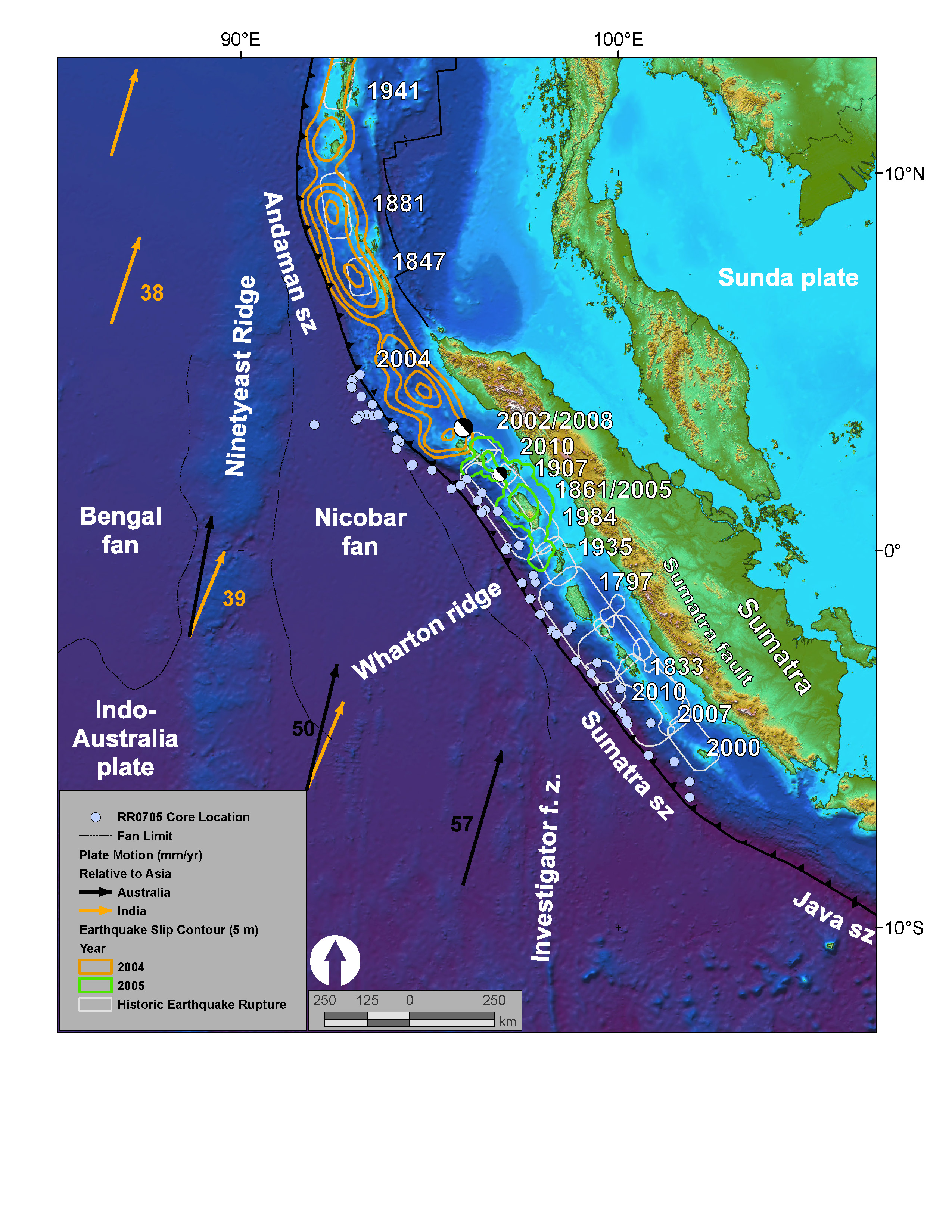
Sumatra core location and plate setting map with sedimentary and erosive systems figure. A. India-Australia plate subducts northeastwardly beneath the Sunda plate (part of Eurasia) at modern rates (GPS velocities are based on regional modeling of Bock et al, 2003 as plotted in Subarya et al., 2006). Historic earthquake ruptures (Bilham, 2005; Malik et al., 2011) are plotted in orange. 2004 earthquake and 2005 earthquake 5 meter slip contours are plotted in orange and green respectively (Chlieh et al., 2007, 2008). Bengal and Nicobar fans cover structures of the India-Australia plate in the northern part of the map. RR0705 cores are plotted as light blue. SRTM bathymetry and topography is in shaded relief and colored vs. depth/elevation (Smith and Sandwell, 1997). B. Schematic illustration of geomorphic elements of subduction zone trench and slope sedimentary settings. Submarine channels, submarine canyons, dune fields and sediment waves, abyssal plain, trench axis, plunge pool, apron fans, and apron fan channels are labeled here. Modified from Patton et al. (2013 a).
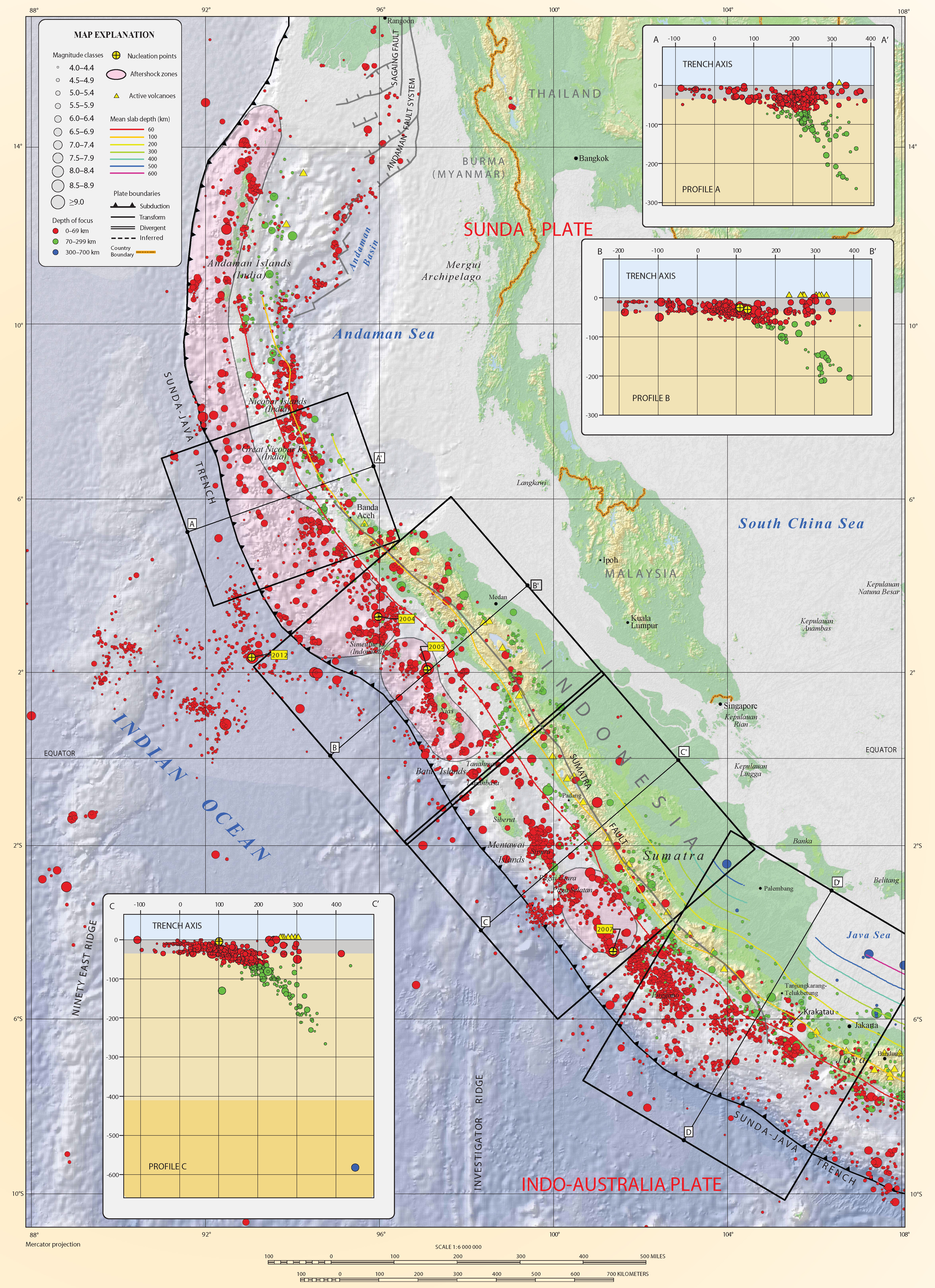
- This is the main figure from Hayes et al. (2013) from the Seismicity of the Earth series. There is a map with the slab contours and seismicity both colored vs. depth. There are also some cross sections of seismicity plotted, with locations shown on the map.
- Here is a great figure from Philobosian et al. (2014) that shows the slip patches from the subduction zone earthquakes in this region.
- This is a figure from Philobosian et al. (2012) that shows a larger scale view for the slip patches in this region. Note that today’s earthquake happened at the edge of the 7.9 earthquake slip patch.

Map of Southeast Asia showing recent and selected historical ruptures of the Sunda megathrust. Black lines with sense of motion are major plate-bounding faults, and gray lines are seafloor fracture zones. Motions of Australian and Indian plates relative to Sunda plate are from the MORVEL-1 global model [DeMets et al., 2010]. The fore-arc sliver between the Sunda megathrust and the strike-slip Sumatran Fault becomes the Burma microplate farther north, but this long, thin strip of crust does not necessarily all behave as a rigid block. Sim = Simeulue, Ni = Nias, Bt = Batu Islands, and Eng = Enggano. Brown rectangle centered at 2°S, 99°E delineates the area of Figure 3, highlighting the Mentawai Islands. Figure adapted from Meltzner et al. [2012] with rupture areas and magnitudes from Briggs et al. [2006], Konca et al. [2008], Meltzner et al. [2010], Hill et al. [2012], and references therein.
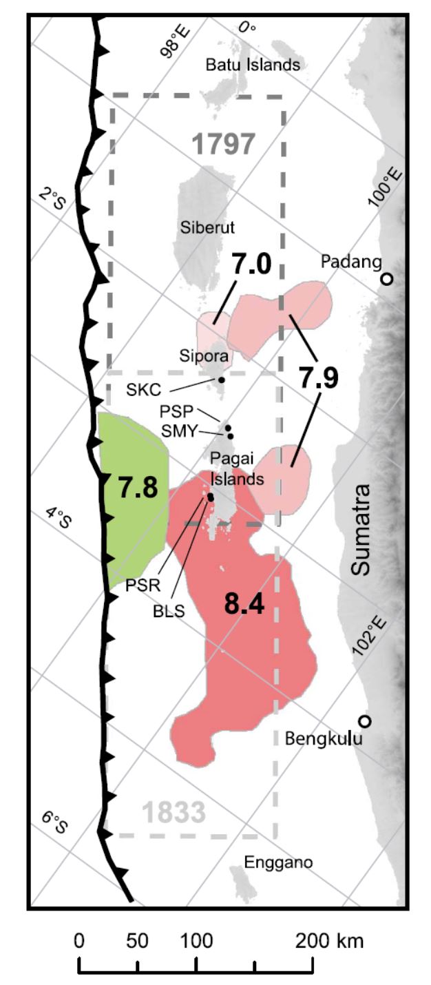
Recent and ancient ruptures along the Mentawai section of the Sunda megathrust. Colored patches are surface projections of 1-m slip contours of the deep megathrust ruptures on 12–13 September 2007 (pink to red) and the shallow rupture on 25 October 2010 (green). Dashed rectangles indicate roughly the sections that ruptured in 1797 and 1833. Ancient ruptures are adapted from Natawidjaja et al. [2006] and recent ones come from Konca et al. [2008] and Hill et al. (submitted manuscript, 2012). Labeled points indicate coral study sites Sikici (SKC), Pasapuat (PSP), Simanganya (SMY), Pulau Pasir (PSR), and Bulasat (BLS).
- Here are a series of figures from Chlieh et al. (2008 ) that show their data sources and their modeling results. I include their figure captions below in blockquote.
- This figure shows the coupling model (on the left) and the source data for their inversions (on the right). Their source data are vertical deformation rates as measured along coral microattols. These are from data prior to the 2004 SASZ earthquake.
- This is a similar figure, but based upon observations between June 2005 and October 2006.
- This is a similar figure, but based on all the data.
- Here is the figure I included in the poster above.
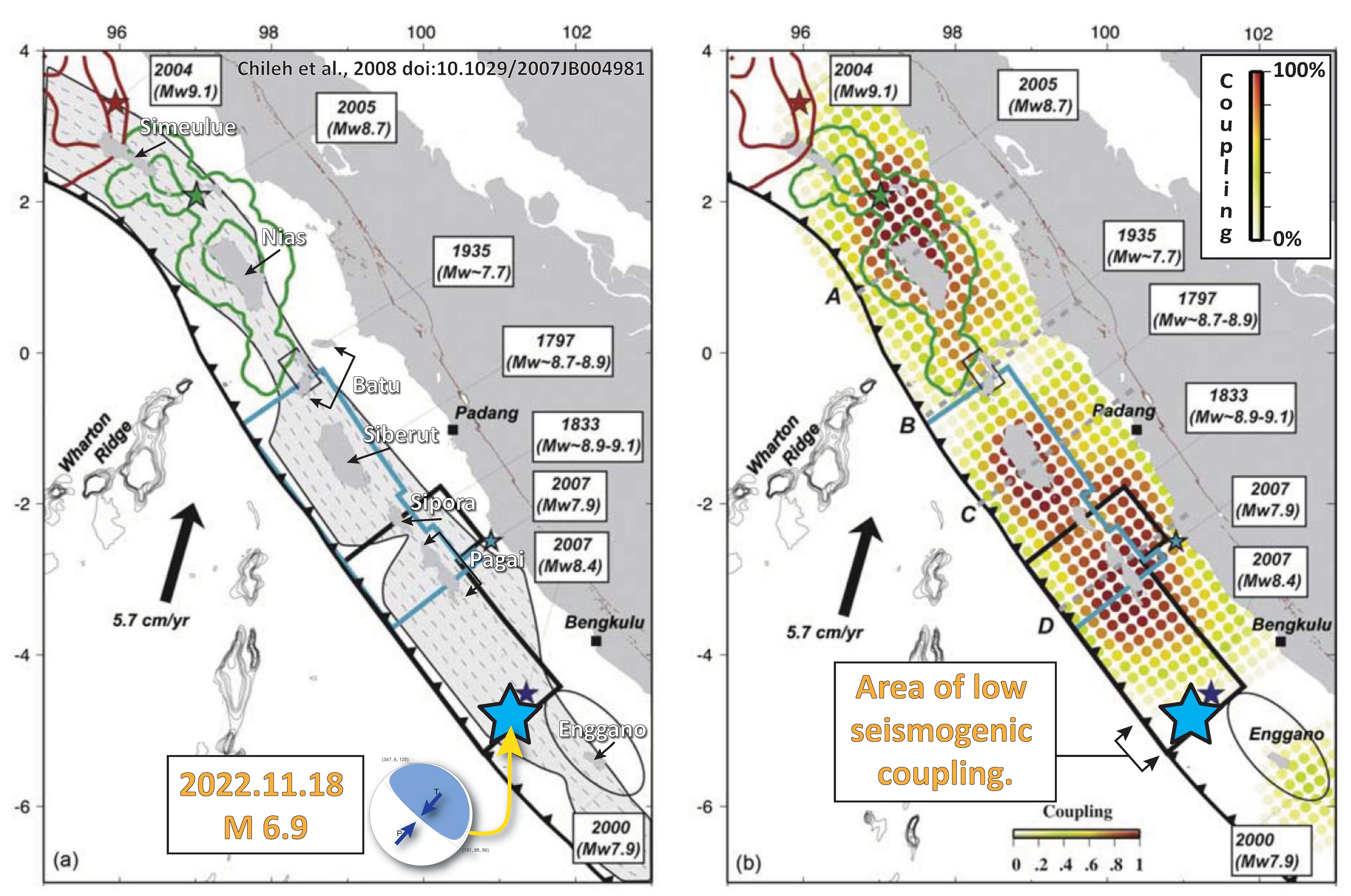
- Here is the Chlieh et al. (2008) figure with the 18 November 2022 M 6.9 earthquake plotted as a blue star.
- Note how the M 6.9 happened in a region of low seismogenic coupling. Beware that this is also in an area without any geodetic (GPS/GNSS) nor paleogeodetic (coral microattol) observations (the sources of data for the coupling model).
- This figure shows the authors’ estimate for the moment deficit in this region of the subduction zone. This is an estimate of how much the plate convergence rate, that is estimated to accumulate as tectonic strain, will need to be released during subduction zone earthquakes.

Distribution of coupling on the Sumatra megathrust derived from the formal inversion of the coral and of the GPS data (Tables 2, 3, and 4) prior to the 2004 Sumatra-Andaman earthquake (model I-a in Table 7). (a) Distribution of coupling on the megathrust. Fully coupled areas are red, and fully creeping areas are white. Three strongly coupled patches are revealed beneath Nias island, Siberut island, and Pagai island. The annual moment deficit rate corresponding to that model is 4.0 X 10^20 N m/a. (b) Observed (black vectors) and predicted (red vectors) horizontal velocities appear. Observed and predicted vertical displacements are shown by color-coded large and small circles, respectively. The Xr^2 of this model is 3.9 (Table 7).
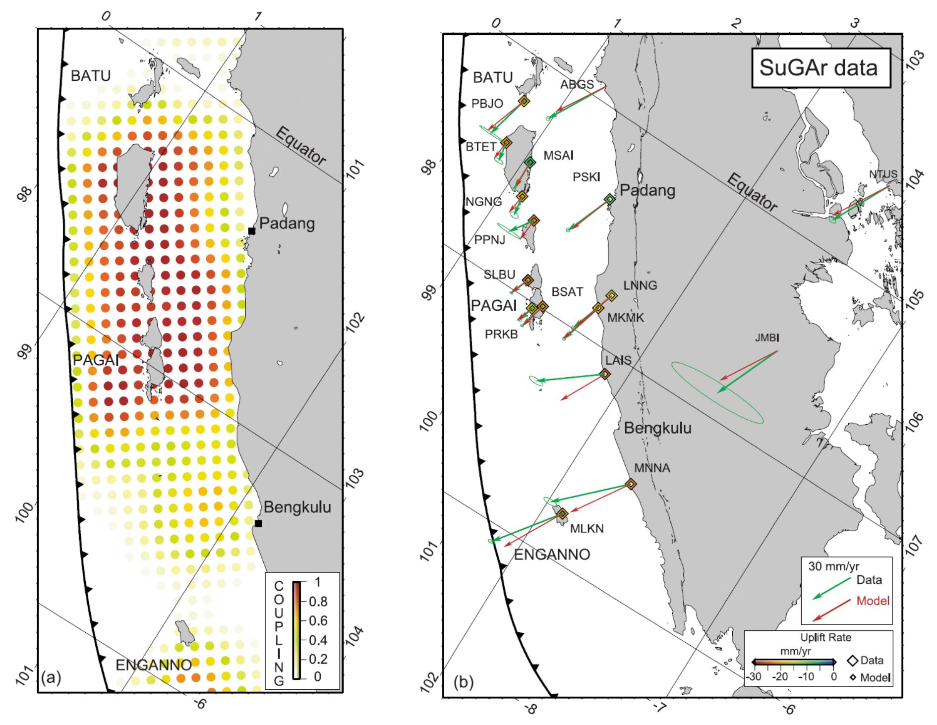
Distribution of coupling on the Sumatra megathrust derived from the formal inversion of the horizontal velocities and uplift rates derived from the CGPS measurements at the SuGAr stations (processed at SOPAC). To reduce the influence of postseismic deformation caused by the March 2005 Nias-Simeulue rupture, velocities were determined for the period between June 2005 and October 2006. (a) Distribution of coupling on the megathrust. Fully coupled areas are red and fully creeping areas are white. This model reveals strong coupling beneath the Mentawai Islands (Siberut, Sipora, and Pagai islands), offshore Padang city, and suggests that the megathrust south of Bengkulu city is creeping at the plate velocity. (b) Comparison of observed (green) and predicted (red) velocities. The Xr^2 associated to that model is 24.5 (Table 8).
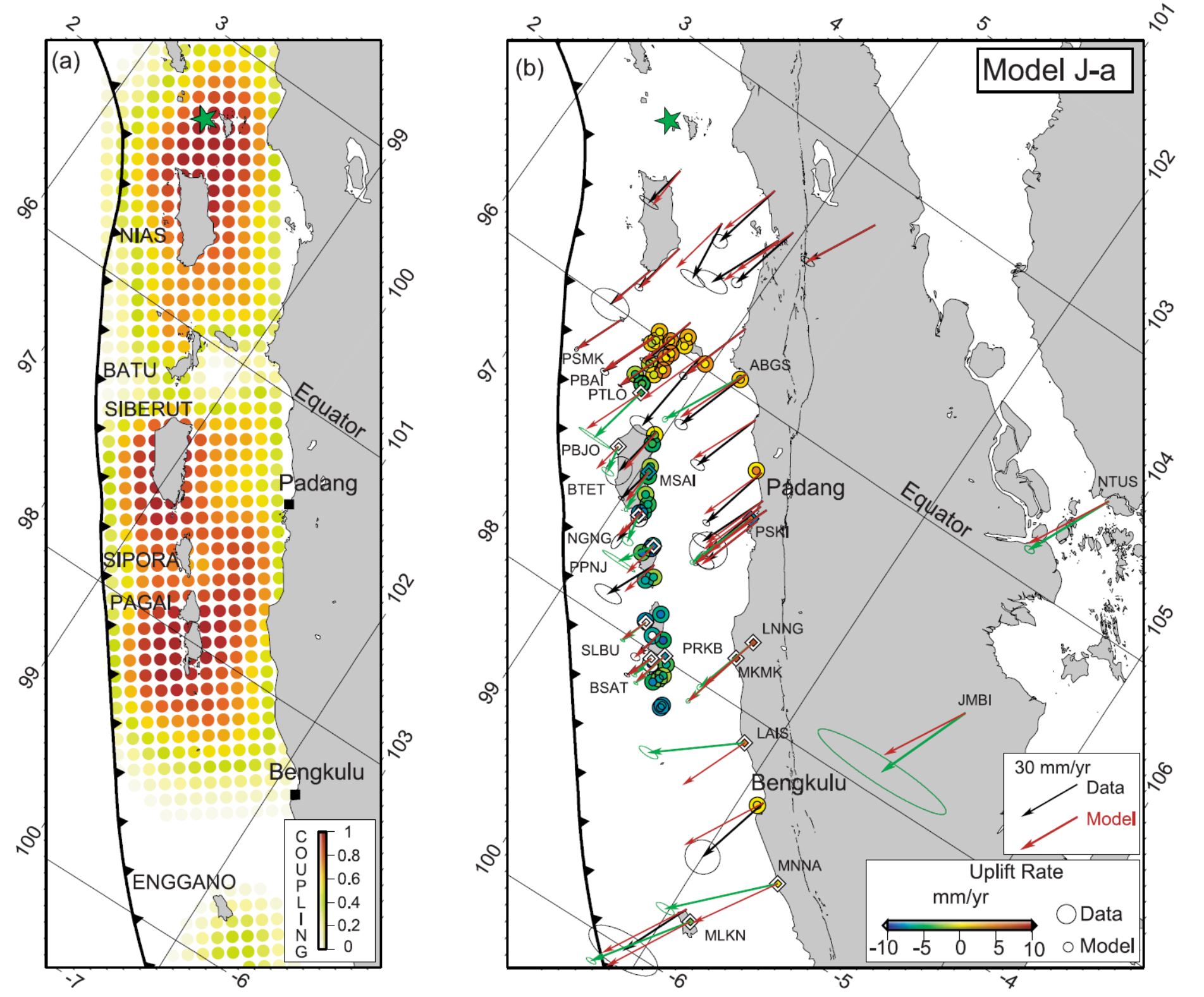
Distribution of coupling on the Sumatra megathrust derived from the formal inversion of all the data (model J-a, Table 8). (a) Distribution of coupling on the megathrust. Fully coupled areas are red, and fully creeping areas are white. This model shows strong coupling beneath Nias island and beneath the Mentawai (Siberut, Sipora and Pagai) islands. The rate of accumulation of moment deficit is 4.5 X 10^20 N m/a. (b) Comparison of observed (black arrows for pre-2004 Sumatra-Andaman earthquake and green arrows for post-2005 Nias earthquake) and predicted velocities (in red). Observed and predicted vertical displacements are shown by color-coded large and small circles (for the corals) and large and small diamonds (for the CGPS), respectively. The Xr^2 of this model is 12.8.
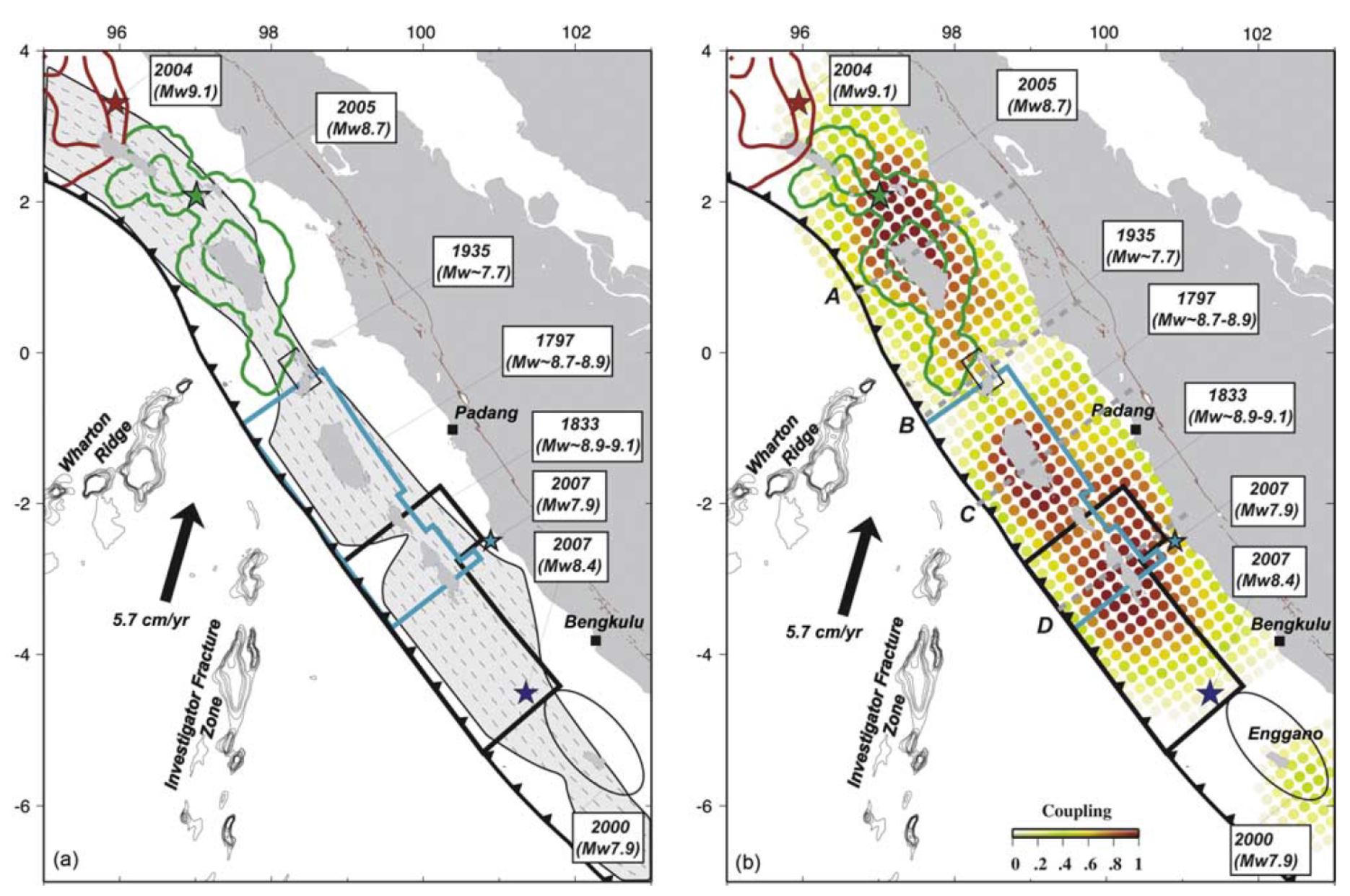
Comparison of interseismic coupling along the megathrust with the rupture areas of the great 1797, 1833, and 2005 earthquakes. The southernmost rupture area of the 2004 Sumatra-Andaman earthquake lies north of our study area and is shown only for reference. Epicenters of the 2007 Mw 8.4 and Mw 7.9 earthquakes are also shown for reference. (a) Geometry of the locked fault zone corresponding to forward model F-f (Figure 6c). Below the Batu Islands, where coupling occurs in a narrow band, the largest earthquake for the past 260 years has been a Mw 7.7 in 1935 [Natawidjaja et al., 2004; Rivera et al., 2002]. The wide zones of coupling, beneath Nias, Siberut, and Pagai islands, coincide well with the source of great earthquakes (Mw > 8.5) in 2005 from Konca et al. [2007] and in 1797 and 1833 from Natawidjaja et al. [2006]. The narrow locked patch beneath the Batu islands lies above the subducting fossil Investigator Fracture Zone. (b) Distribution of interseismic coupling corresponding to inverse model J-a (Figure 10). The coincidence of the high coupling area (orange-red dots) with the region of high coseismic slip during the 2005 Nias-Simeulue earthquake suggests that strongly coupled patches during interseismic correspond to seismic asperities during megathrust ruptures. The source regions of the 1797 and 1833 ruptures also correlate well with patches that are highly coupled beneath Siberut, Sipora, and Pagai islands.
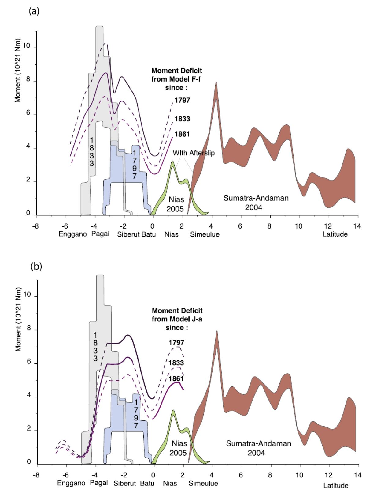
Latitudinal distributions of seismic moment released by great historical earthquakes and of accumulated deficit of moment due to interseismic locking of the plate interface. Values represent integrals over half a degree of latitude. Accumulated interseismic deficits since 1797, 1833, and 1861 are based on (a) model F-f and (b) model J-a. Seismic moments for the 1797 and 1833 Mentawai earthquakes are estimated based on the work by Natawidjaja et al. [2006], the 2005 Nias-Simeulue earthquake is taken from Konca et al. [2007], and the 2004 Sumatra-Andaman earthquake is taken from Chlieh et al. [2007]. Postseismic moments released in the month that follows the 2004 earthquake and in the 11 months that follows the Nias-Simeulue 2005 earthquake are shown in red and green, respectively, based on the work by Chlieh et al. [2007] and Hsu et al. [2006].
- For a review of the 2004 and 2005 Sumatra Andaman subduction zone (SASZ) earthquakes, please check out my Earthquake Report here. Below is the poster from that report. On that report page, I also include some information about the 2012 M 8.6 and M 8.2 Wharton Basin earthquakes.
- I include some inset figures in the poster.
- In the upper left corner, I include a map that shows the extent of historic earthquakes along the SASZ offshore of Sumatra. This map is a culmination of a variety of papers (summarized and presented in Patton et al., 2015).
- In the upper right corner I include a figure that is presented by Chlieh et al. (2007). These figures show model results from several models. Each model is represented by a map showing the amount that the fault slipped in particular regions. I present this figure below.
- In the lower right corner I present a figure from Prawirodirdjo et al. (2010). This figure shows the coseismic vertical and horizontal motions from the 2004 and 2005 earthquakes as measured at GPS sites.
- In the lower left corner are the MMI intensity maps for the two SASZ earthquakes. Note these are at different map scales. I also include the MMI attenuation curves for these earthquakes below the maps. These plots show the reported MMI intensity data as they relate to two plots of modeled estimates (the orange and green lines). These green dots are from the USGS “Did You Feel It?” reports compared to the estimates of ground shaking from Ground Motion Prediction Equation (GMPE) estimates. GMPE are empirical relations between earthquakes and recorded seismologic observations from those earthquakes, largely controlled by distance to the fault, ray path (direction and material properties), and site effects (the local geology). When seismic waves propagate through sediment, the magnitude of the ground motions increases in comparison to when seismic waves propagate through bedrock. The orange line is a regression of data for the central and eastern US and the green line is a regression through data from the western US.
- Here is a map from Jacob et a. (2014) that shows the structure of the eastern Indian Ocean. Figure text below.
- Here is the map from Jacobs et a. (2014). Figure text below.
- This is a fascinating figure from Jacob et al. (2014). This shows a reconstruction of the magntic anomalies for the oceanic crust as they are subducted beneath Eurasia.
- Finally, these authors present what their reconstruction implicates about this plate boundary system.
Free-air gravity anomaly map derived from satellite altimetry [Sandwell and Smith, 2009] over the Wharton Basin area.
Structure and age of the Wharton Basin deduced from free-air gravity anomaly [Sandwell and Smith, 2009; background colors] for the fracture zones (thin black longitudinal lines), and marine magnetic anomaly profiles (not shown) for the isochrons (thin black latitudinal lines). The plain colors represent the oceanic lithosphere created during normal geomagnetic polarity intervals (see legend for the ages of Chrons 20 to 34 according to the time scale of Gradstein et al. [2004]). Compartments separated by major fracture zones are labeled A to H. Grey areas: oceanic plateaus, thick black line: Sunda Trench subduction zone.
Reconstitution of the subducted magnetic isochrons and fracture zones of the northern Wharton Basin using the finite rotation parameters deduced from our two- and three-plate reconstructions. (a) First the geometry is restored on the Earth surface, then (b) it is draped on the top of the subducting plate as derived from seismic tomography [Pesicek et al., 2010] shown by the thin dotted lines at intervals of 100 km (b). Colored dots: identified magnetic anomalies; colored triangles: rotated magnetic anomalies, solid lines; observed fracture zones and isochrons, dashed lines: uncertain or reconstructed fracture zones, dotted lines: reconstructed isochrons from rotated magnetic anomalies (two-plate and three-plate reconstructions), colored area: oceanic lithosphere created during normal geomagnetic polarity intervals (see legend for the ages; the colored areas without solid or dotted lines have been interpolated), grey areas: oceanic plateaus, thick line: Sunda Trench subduction zone.

The deviation of the Sunda Trench from a regular arc shape (dotted lines) off Sumatra is explained by the presence of the younger, hotter and therefore lighter lithosphere in compartments C–F, which resists subduction and form an indentor (solid line). The very young compartment G was probably part of this indentor before oceanic crust formed at slow spreading rate near the Wharton fossil spreading center approached subduction: The weaker rheology of outcropping or shallow serpentinite may have favored the restoration of the accretionary prism in this area. Further south, the deviation off Java is explained by the resistance of the thicker Roo Rise, an oceanic plateau entering the subduction.
Seismic Hazard and Seismic Risk
- These are the two maps shown in the map above, the GEM Seismic Hazard and the GEM Seismic Risk maps from Pagani et al. (2018) and Silva et al. (2018).
- The GEM Seismic Hazard Map:
- The Global Earthquake Model (GEM) Global Seismic Hazard Map (version 2018.1) depicts the geographic distribution of the Peak Ground Acceleration (PGA) with a 10% probability of being exceeded in 50 years, computed for reference rock conditions (shear wave velocity, VS30, of 760-800 m/s). The map was created by collating maps computed using national and regional probabilistic seismic hazard models developed by various institutions and projects, and by GEM Foundation scientists. The OpenQuake engine, an open-source seismic hazard and risk calculation software developed principally by the GEM Foundation, was used to calculate the hazard values. A smoothing methodology was applied to homogenise hazard values along the model borders. The map is based on a database of hazard models described using the OpenQuake engine data format (NRML). Due to possible model limitations, regions portrayed with low hazard may still experience potentially damaging earthquakes.
- Here is a view of the GEM seismic hazard map for Indonesia.
- The GEM Seismic Risk Map:
- The Global Seismic Risk Map (v2018.1) presents the geographic distribution of average annual loss (USD) normalised by the average construction costs of the respective country (USD/m2) due to ground shaking in the residential, commercial and industrial building stock, considering contents, structural and non-structural components. The normalised metric allows a direct comparison of the risk between countries with widely different construction costs. It does not consider the effects of tsunamis, liquefaction, landslides, and fires following earthquakes. The loss estimates are from direct physical damage to buildings due to shaking, and thus damage to infrastructure or indirect losses due to business interruption are not included. The average annual losses are presented on a hexagonal grid, with a spacing of 0.30 x 0.34 decimal degrees (approximately 1,000 km2 at the equator). The average annual losses were computed using the event-based calculator of the OpenQuake engine, an open-source software for seismic hazard and risk analysis developed by the GEM Foundation. The seismic hazard, exposure and vulnerability models employed in these calculations were provided by national institutions, or developed within the scope of regional programs or bilateral collaborations.
- Here is a view of the GEM seismic risk map for Indonesia.

Tsunami Hazard
- Here are two maps that show the results of probabilistic tsunami modeling for the nation of Indonesia (Horspool et al., 2014). These results are similar to results from seismic hazards analysis and maps. The color represents the chance that a given area will experience a certain size tsunami (or larger).
- The first map shows the annual chance of a tsunami with a height of at least 0.5 m (1.5 feet). The second map shows the chance that there will be a tsunami at least 3 meters (10 feet) high at the coast.
Annual probability of experiencing a tsunami with a height at the coast of (a) 0.5m (a tsunami warning) and (b) 3m (a major tsunami warning).
- M 9.2 Andaman-Sumatra subduction zone 2014 Earthquake Anniversary
- M 9.2 Andaman-Sumatra subduction zone SASZ Fault Deformation
- M 9.2 Andaman-Sumatra subduction zone 2016 Earthquake Anniversary
- 2023.04.24 M 7.1 Sumatra
- 2022.11.18 M 6.9 Sumatra
- 2022.02.25 M 6.2 Sumatra
- 2020.05.06 M 6.8 Banda Sea
- 2019.08.02 M 6.9 Indonesia
- 2019.06.23 M 7.3 Banda Sea
- 2019.04.12 M 6.8 Sulawesi, Indonesia
- 2018.09.28 M 7.5 Sulawesi
- 2018.10.16 M 7.5 Sulawesi UPDATE #1
- 2018.08.19 M 6.9 Lombok, Indonesia
- 2018.08.05 M 6.9 Lombok, Indonesia
- 2018.07.28 M 6.4 Lombok, Indonesia
- 2017.12.15 M 6.5 Java
- 2017.08.31 M 6.3 Mentawai, Sumatra
- 2017.08.13 M 6.4 Bengkulu, Sumatra, Indonesia
- 2017.05.29 M 6.8 Sulawesi, Indonesia
- 2017.03.14 M 6.0 Sumatra
- 2017.03.01 M 5.5 Banda Sea
- 2016.10.19 M 6.6 Java
- 2016.03.02 M 7.8 Sumatra/Indian Ocean
- 2015.07.22 M 5.8 Andaman Sea
- 2015.11.08 M 6.4 Nicobar Isles
- 2012.04.11 M 8.6 Sumatra outer rise
- 2004.12.26 M 9.2 Andaman-Sumatra subduction zone
Indonesia | Sumatra
General Overview
Earthquake Reports
Social Media
#EarthquakeReport for M7.1 #Gempa #Earthquake offshore of #Sumatra #Indonesia
Strong ground shaking w felt reports of intensity MMI 9
must have been terrifying
Hopefully there is little sufferingLearn more from earlier report https://t.co/KKizpqrU0Chttps://t.co/b9naiPPnbA pic.twitter.com/ThnHCzPNxv
— Jason "Jay" R. Patton (@patton_cascadia) April 24, 2023
#EarthquakeReport for M7.1 #Gempa #Earthquake offshore of #Sumatra #Indonesia @USGS_Quakes model results show the likelihood (chance) for liquefaction induced by the earthquake
Learn more from earlier report https://t.co/MsVJ54GpGMhttps://t.co/s269GrVReM pic.twitter.com/cZ2EjlRHb1
— Jason "Jay" R. Patton (@patton_cascadia) April 24, 2023
#EarthquakeReport for M7.1 #Gempa #Earthquake offshore of #Sumatra #Indonesia
felt reports of intensity MMI 9
This plot shows how earthquake intensity gets smaller w/distance
Learn more from earlier report https://t.co/MsVJ54GpGMhttps://t.co/ROpl0cNYYx pic.twitter.com/pGuafAWLxN
— Jason "Jay" R. Patton (@patton_cascadia) April 24, 2023
#EarthquakeReport for M7.1 #Gempa #Earthquake offshore of Batu Islands, Siberut Island, and #Sumatra #Indonesia
megathrust subduction zone earthquake
likely generated a modest local tsunami
potential for ground failureinterpretive poster and report herehttps://t.co/yATr1rEugZ pic.twitter.com/3S6OeT3mow
— Jason "Jay" R. Patton (@patton_cascadia) April 25, 2023
— Jason "Jay" R. Patton (@patton_cascadia) April 24, 2023
M 7.1 – 170 km SSE of Teluk Dalam, Indonesiahttps://t.co/7jWUUYLp7E pic.twitter.com/n83OgwYCmj
— Wendy Bohon, PhD 🌏 (@DrWendyRocks) April 24, 2023
#Earthquake (#gempa) confirmed by seismic data.⚠Preliminary info: M6.7 || 174 km W of #Pariaman (#Indonesia) || 9 min ago (local time 03:00:54). Follow the thread for the updates👇 pic.twitter.com/T0fEZEoE6j
— EMSC (@LastQuake) April 24, 2023
#Earthquake in #Indonesia – Early impact estimation. Modified Mercalli Intensity: 7.0/10 – Population Exposure Estim.: https://t.co/BPHYunonh4 pic.twitter.com/ONbpUUpzdd
— ADAM Disaster Alerts (@WFP_ADAM) April 24, 2023
Major M7ish, shallow, upslip (reverse) faulting #earthquake on Australian-Sunda (Pacific) plates boundary with 5-6cm/y convergence. Potential for local land and mud slides and perhaps minor tsunami impact. Region known for recent great earthquakes.#geohazards #Indonesia https://t.co/7h2pOcX1TV pic.twitter.com/GG6kF7lg5Z
— 🌎 Prof Ben van der Pluijm ⚒️ (@vdpluijm) April 24, 2023
Watch the waves from the M7.1 Sumatra, Indonesia earthquake roll across seismic stations in North America.
More info⬇️ pic.twitter.com/DW7qzpRwjm
— EarthScope Consortium (@EarthScope_sci) April 25, 2023
2023-04-24 M7.1 #Indonesia #earthquake recorded in #Scotland + historical seismicity & cross section.
Weak P/PcP arrival on many stations & clear surface waves for most (2nd plot).
Dist: 10889km
Travel Time: 13m 37s
Depth: 15km#Python @raspishake @matplotlib #CitizenScience pic.twitter.com/EzZMkYa1W8— Giuseppe Petricca (@gmrpetricca) April 25, 2023
M7.1 earthquake near Indonesia at 20.00 UTC on 24 April 2023. Recorded in Nottingham using horizontal pendulum school seismometer from @mindsets_uk #earthquake https://t.co/wQVD8D7eVg pic.twitter.com/rSPebaQ0YZ
— Geological Outreach (@GeoOutreach) April 24, 2023
Large earthquake near Indonesia, preliminary information suggests M6.7-M6.9 and shallow depth. Based on early depths and epicenter, this could be a shallow subduction interface event. https://t.co/1x9UBcPEZx pic.twitter.com/qkiOfaqwzA
— Jascha Polet (@CPPGeophysics) April 24, 2023
Pretty decent size earthquake this morning, I am currently at my in laws, a little bit to the southeast of Padang but it didn't woke me up although my in laws said they felt a strong swaying, stay safe everyone on the outer islands 🙏 pic.twitter.com/8PVekovYEC
— Gayatri Marliyani (@GMarliyani) April 24, 2023
Karakteristik Gempa Megathrust dengan mekanisme naik (thrust fault) di bidang kontak antar lempeng di kedalaman 23 km. pic.twitter.com/ORbJymysj8
— DARYONO BMKG (@DaryonoBMKG) April 24, 2023
Sebelum terjadi gempa dengan skala 7 pagi hari ini. Setidaknya telah terjadi beberapa kali gempa preshock yang mendahului sejak 2 hari yang lalu (23 April 2023) pic.twitter.com/iUmYYMUgyt
— INFOMITIGASI™ (@infomitigasi) April 24, 2023
Recent Earthquake Teachable Moment for the M7.1 Indonesia earthquake.
Teachable Moments presentations capture the opportunity to bring knowledge, insight, and critical thinking to the classroom following a newsworthy earthquake.https://t.co/NrmdZ6Xu2Y pic.twitter.com/dzUpYiC0LR
— EarthScope Consortium (@EarthScope_sci) April 25, 2023
The magnitude-7.1 earthquake that struck off the coast of Sumatra earlier today occurred at the edge of a seismic gap. Asst Prof Meltzner @QuakesAndShakes said that we are still expecting a great earthquake in the region in the future. Find out more at https://t.co/3jYBFB8MBx
— Earth Observatory SG (@EOS_SG) April 25, 2023
- Frisch, W., Meschede, M., Blakey, R., 2011. Plate Tectonics, Springer-Verlag, London, 213 pp.
- Hayes, G., 2018, Slab2 – A Comprehensive Subduction Zone Geometry Model: U.S. Geological Survey data release, https://doi.org/10.5066/F7PV6JNV.
- Holt, W. E., C. Kreemer, A. J. Haines, L. Estey, C. Meertens, G. Blewitt, and D. Lavallee (2005), Project helps constrain continental dynamics and seismic hazards, Eos Trans. AGU, 86(41), 383–387, , https://doi.org/10.1029/2005EO410002. /li>
- Jessee, M.A.N., Hamburger, M. W., Allstadt, K., Wald, D. J., Robeson, S. M., Tanyas, H., et al. (2018). A global empirical model for near-real-time assessment of seismically induced landslides. Journal of Geophysical Research: Earth Surface, 123, 1835–1859. https://doi.org/10.1029/2017JF004494
- Kreemer, C., J. Haines, W. Holt, G. Blewitt, and D. Lavallee (2000), On the determination of a global strain rate model, Geophys. J. Int., 52(10), 765–770.
- Kreemer, C., W. E. Holt, and A. J. Haines (2003), An integrated global model of present-day plate motions and plate boundary deformation, Geophys. J. Int., 154(1), 8–34, , https://doi.org/10.1046/j.1365-246X.2003.01917.x.
- Kreemer, C., G. Blewitt, E.C. Klein, 2014. A geodetic plate motion and Global Strain Rate Model in Geochemistry, Geophysics, Geosystems, v. 15, p. 3849-3889, https://doi.org/10.1002/2014GC005407.
- Meyer, B., Saltus, R., Chulliat, a., 2017. EMAG2: Earth Magnetic Anomaly Grid (2-arc-minute resolution) Version 3. National Centers for Environmental Information, NOAA. Model. https://doi.org/10.7289/V5H70CVX
- Müller, R.D., Sdrolias, M., Gaina, C. and Roest, W.R., 2008, Age spreading rates and spreading asymmetry of the world’s ocean crust in Geochemistry, Geophysics, Geosystems, 9, Q04006, https://doi.org/10.1029/2007GC001743
- Pagani,M. , J. Garcia-Pelaez, R. Gee, K. Johnson, V. Poggi, R. Styron, G. Weatherill, M. Simionato, D. Viganò, L. Danciu, D. Monelli (2018). Global Earthquake Model (GEM) Seismic Hazard Map (version 2018.1 – December 2018), DOI: 10.13117/GEM-GLOBAL-SEISMIC-HAZARD-MAP-2018.1
- Silva, V ., D Amo-Oduro, A Calderon, J Dabbeek, V Despotaki, L Martins, A Rao, M Simionato, D Viganò, C Yepes, A Acevedo, N Horspool, H Crowley, K Jaiswal, M Journeay, M Pittore, 2018. Global Earthquake Model (GEM) Seismic Risk Map (version 2018.1). https://doi.org/10.13117/GEM-GLOBAL-SEISMIC-RISK-MAP-2018.1
- Zhu, J., Baise, L. G., Thompson, E. M., 2017, An Updated Geospatial Liquefaction Model for Global Application, Bulletin of the Seismological Society of America, 107, p 1365-1385, https://doi.org/0.1785/0120160198
- Andrade, V. and Rajendran, K., 2014. The April 2012 Indian Ocean earthquakes: Seismotectonic context and implications for their mechanisms in Tectonophysics, v. 617, p. 126-139, http://dx.doi.org/10.1016/j.tecto.2014.01.024
- Heidarzadeh, M., Harada, T., Satake, K., Ishibe, T., Takagawa, T., 2017. Tsunamis from strike-slip earthquakes in the Wharton Basin, northeast Indian Ocean: March 2016 Mw7.8 event and its relationship with the April 2012 Mw 8.6 event in GJI, v. 2110, p. 1601-1612, doi: 10.1093/gji/ggx395
- Jacob, J., J. Dyment, and V. Yatheesh, 2014. Revisiting the structure, age, and evolution of the Wharton Basin to better understand subduction under Indonesia, J. Geophys. Res. Solid Earth, 119, 169–190, doi:10.1002/2013JB010285.
- Yadav, R.K., Kundu, B., Gahalaut, K., Catherine, J., Gahalaut, V.K., Ambikapathy, A., and Naidu, MZ.S., 2013. Coseismic offsets due to the 11 April 2012 Indian Ocean earthquakes (Mw 8.6 and 8.2) derived from GPS measurements in Geophysical Research Letters, v. 40, p. 3389-3393, doi:10.1002/grl.50601
- Wiseman, K. and Bürgmann, R., 2012. Stress triggering of the great Indian Ocean strike-slip earthquakes in a diffuse plate boundary zone in Geophysical research Letters, v. 39, L22304, doi:10.1029/2012GL053954
- Abercrombie, R.E., Antolik, M., Ekstrom, G., 2003. The June 2000 Mw 7.9 earthquakes south of Sumatra: Deformation in the India–Australia Plate. Journal of Geophysical Research 108, 16.
- Bassin, C., Laske, G. and Masters, G., The Current Limits of Resolution for Surface Wave Tomography in North America, EOS Trans AGU, 81, F897, 2000.
- Bock, Y., Prawirodirdjo, L., Genrich, J.F., Stevens, C.W., McCaffrey, R., Subarya, C., Puntodewo, S.S.O., Calais, E., 2003. Crustal motion in Indonesia from Global Positioning System measurements: Journal of Geophysical Research, v. 108, no. B8, 2367, doi: 10.1029/2001JB000324.
- Bothara, J., Beetham, R.D., Brunston, D., Stannard, M., Brown, R., Hyland, C., Lewis, W., Miller, S., Sanders, R., Sulistio, Y., 2010. General observations of effects of the 30th September 2009 Padang earthquake, Indonesia. Bulletin of the New Zealand Society for Earthquake Engineering 43, 143-173.
- Chlieh, M., Avouac, J.-P., Hjorleifsdottir, V., Song, T.-R.A., Ji, C., Sieh, K., Sladen, A., Hebert, H., Prawirodirdjo, L., Bock, Y., Galetzka, J., 2007. Coseismic Slip and Afterslip of the Great (Mw 9.15) Sumatra-Andaman Earthquake of 2004. Bulletin of the Seismological Society of America 97, S152-S173.
- Chlieh, M., Avouac, J.P., Sieh, K., Natawidjaja, D.H., Galetzka, J., 2008. Heterogeneous coupling of the Sumatran megathrust constrained by geodetic and paleogeodetic measurements: Journal of Geophysical Research, v. 113, B05305, doi: 10.1029/2007JB004981.
- DEPLUS, C. et al., 1998 – Direct evidence of active derormation in the eastern Indian oceanic plate, Geology.
- DYMENT, J., CANDE, S.C. & SINGH, S., 2007 – Oceanic lithosphere subducting beneath the Sunda Trench: the Wharton Basin revisited. European Geosciences Union General Assembly, Vienna, 15-20/05.
- Hayes, G. P., Wald, D. J., and Johnson, R. L., 2012. Slab1.0: A three-dimensional model of global subduction zone geometries in J. Geophys. Res., 117, B01302, doi:10.1029/2011JB008524.
- Hayes, G.P., Bernardino, Melissa, Dannemann, Fransiska, Smoczyk, Gregory, Briggs, Richard, Benz, H.M., Furlong, K.P., and Villaseñor, Antonio, 2013. Seismicity of the Earth 1900–2012 Sumatra and vicinity: U.S. Geological Survey Open-File Report 2010–1083-L, scale 1:6,000,000, https://pubs.usgs.gov/of/2010/1083/l/.
- JACOB, J., DYMENT, J., YATHEESH, V. & BHATTACHARYA, G.C., 2009 – Marine magnetic anomalies in the NE Indian Ocean: the Wharton and Central Indian basins revisited. European Geosciences Union General Assembly, Vienna, 19-24/04.
- Ji, C., D.J. Wald, and D.V. Helmberger, Source description of the 1999 Hector Mine, California earthquake; Part I: Wavelet domain inversion theory and resolution analysis, Bull. Seism. Soc. Am., Vol 92, No. 4. pp. 1192-1207, 2002.
- Ishii, M., Shearer, P.M., Houston, H., Vidale, J.E., 2005. Extent, duration and speed of the 2004 Sumatra-Andaman earthquake imaged by the Hi-Net array. Nature 435, 933.
- Kanamori, H., Rivera, L., Lee, W.H.K., 2010. Historical seismograms for unravelling a mysterious earthquake: The 1907 Sumatra Earthquake. Geophysical Journal International 183, 358-374.
- Konca, A.O., Avouac, J., Sladen, A., Meltzner, A.J., Sieh, K., Fang, P., Li, Z., Galetzka, J., Genrich, J., Chlieh, M., Natawidjaja, D.H., Bock, Y., Fielding, E.J., Ji, C., Helmberger, D., 2008. Partial Rupture of a Locked Patch of the Sumatra Megathrust During the 2007 Earthquake Sequence. Nature 456, 631-635.
- Maus, S., et al., 2009. EMAG2: A 2–arc min resolution Earth Magnetic Anomaly Grid compiled from satellite, airborne, and marine magnetic measurements, Geochem. Geophys. Geosyst., 10, Q08005, doi:10.1029/2009GC002471.
- Malik, J.N., Shishikura, M., Echigo, T., Ikeda, Y., Satake, K., Kayanne, H., Sawai, Y., Murty, C.V.R., Dikshit, D., 2011. Geologic evidence for two pre-2004 earthquakes during recent centuries near Port Blair, South Andaman Island, India: Geology, v. 39, p. 559-562.
- Meltzner, A.J., Sieh, K., Chiang, H., Shen, C., Suwargadi, B.W., Natawidjaja, D.H., Philobosian, B., Briggs, R.W., Galetzka, J., 2010. Coral evidence for earthquake recurrence and an A.D. 1390–1455 cluster at the south end of the 2004 Aceh–Andaman rupture. Journal of Geophysical Research 115, 1-46.
- Meng, L., Ampuero, J.-P., Stock, J., Duputel, Z., Luo, Y., and Tsai, V.C., 2012. Earthquake in a Maze: Compressional Rupture Branching During the 2012 Mw 8.6 Sumatra Earthquake in Science, v. 337, p. 724-726.
- Natawidjaja, D.H., Sieh, K., Chlieh, M., Galetzka, J., Suwargadi, B., Cheng, H., Edwards, R.L., Avouac, J., Ward, S.N., 2006. Source parameters of the great Sumatran megathrust earthquakes of 1797 and 1833 inferred from coral microatolls. Journal of Geophysical Research 111, 37.
- Newcomb, K.R., McCann, W.R., 1987. Seismic History and Seismotectonics of the Sunda Arc. Journal of Geophysical Research 92, 421-439.
- Philibosian, B., Sieh, K., Natawidjaja, D.H., Chiang, H., Shen, C., Suwargadi, B., Hill, E.M., Edwards, R.L., 2012. An ancient shallow slip event on the Mentawai segment of the Sunda megathrust, Sumatra. Journal of Geophysical Research 117, 12.
- Prawirodirdjo, P., McCaffrey,R., Chadwell, D., Bock, Y, and Subarya, C., 2010. Geodetic observations of an earthquake cycle at the Sumatra subduction zone: Role of interseismic strain segmentation, JOURNAL OF GEOPHYSICAL RESEARCH, v. 115, B03414, doi:10.1029/2008JB006139
- Rivera, L., Sieh, K., Helmberger, D., Natawidjaja, D.H., 2002. A Comparative Study of the Sumatran Subduction-Zone Earthquakes of 1935 and 1984. BSSA 92, 1721-1736.
- Shearer, P., and Burgmann, R., 2010. Lessons Learned from the 2004 Sumatra-Andaman Megathrust Rupture, Annu. Rev. Earth Planet. Sci. v. 38, pp. 103–31
- SATISH C. S, CARTON H, CHAUHAN A.S., et al., 2011 – Extremely thin crust in the Indian Ocean possibly resulting from Plume-Ridge Interaction, Geophysical Journal International.
- Sieh, K., Natawidjaja, D.H., Meltzner, A.J., Shen, C., Cheng, H., Li, K., Suwargadi, B.W., Galetzka, J., Philobosian, B., Edwards, R.L., 2008. Earthquake Supercycles Inferred from Sea-Level Changes Recorded in the Corals of West Sumatra. Science 322, 1674-1678.
- Singh, S.C., Carton, H.L., Tapponnier, P, Hananto, N.D., Chauhan, A.P.S., Hartoyo, D., Bayly, M., Moeljopranoto, S., Bunting, T., Christie, P., Lubis, H., and Martin, J., 2008. Seismic evidence for broken oceanic crust in the 2004 Sumatra earthquake epicentral region, Nature Geoscience, v. 1, pp. 5.
- Smith, W.H.F., Sandwell, D.T., 1997. Global seafloor topography from satellite altimetry and ship depth soundings: Science, v. 277, p. 1,957-1,962.
- Sorensen, M.B., Atakan, K., Pulido, N., 2007. Simulated Strong Ground Motions for the Great M 9.3 Sumatra–Andaman Earthquake of 26 December 2004. BSSA 97, S139-S151.
- Subarya, C., Chlieh, M., Prawirodirdjo, L., Avouac, J., Bock, Y., Sieh, K., Meltzner, A.J., Natawidjaja, D.H., McCaffrey, R., 2006. Plate-boundary deformation associated with the great Sumatra–Andaman earthquake: Nature, v. 440, p. 46-51.
- Tolstoy, M., Bohnenstiehl, D.R., 2006. Hydroacoustic contributions to understanding the December 26th 2004 great Sumatra–Andaman Earthquake. Survey of Geophysics 27, 633-646.
- Zhu, Lupei, and Donald V. Helmberger. “Advancement in source estimation techniques using broadband regional seismograms.” Bulletin of the Seismological Society of America 86.5 (1996): 1634-1641.
References:
Basic & General References
Specific References
Return to the Earthquake Reports page.
- Sorted by Magnitude
- Sorted by Year
- Sorted by Day of the Year
- Sorted By Region