
There was a magnitude M 6.2 Gempa or Earthquake on 25 February 2022.
https://earthquake.usgs.gov/earthquakes/eventpage/us6000gzyg/executive
The plate boundary fault system that dominates the tectonics of the Island of Sumatera, Indonesia, is the complicated.
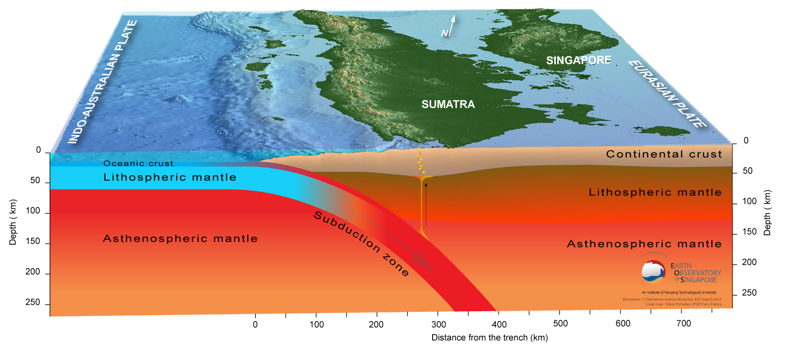
The oceanic India-Australia plate converges with the Eurasia plate to form the Sunda trench. This convergent plate boundary forms a subduction zone where the oceanic plate subducts beneath the continental plate.
Below is a low-angle oblique view cut into the Earth showing this plate configuration from the Earth Observatory Singapore.
However, the direction of plate convergence is not perpendicular to the plate boundary fault (the megathrust subduction zone). Why does this matter?
Because the convergence is at an angle oblique to the plate boundary, we can imagine that this convergence can be subdivided into two components of motion:
- the fault perpendicular motion
- and the fault parallel motion
The amount of plate convergence that is perpendicular to the plate boundary is accommodated by earthquake fault slip on the megathrust.
The amount of plate convergence that is parallel to the plate boundary is accommodated by earthquake fault slip on a different series of faults that we call sliver faults. The Great Sumatra fault is one of these [forearc] sliver faults.
Here is a figure from Lange et al. (2008) that shows how oblique plate convergence forms both a subduction zone and a forearc sliver fault system.

The M 6.2 earthquake is a strike-slip earthquake along the Great Sumatra fault, one of these forearc sliver faults.
Based on our knowledge of this fault system and the earthquake mechanism, we can easily interpret this to be a right-lateral strike-slip fault.
There are numerous historical analogies from the past century. Most of the events in the past few decades have been in the M 6-7 range, though there have been events of larger magnitude in the past centuries.
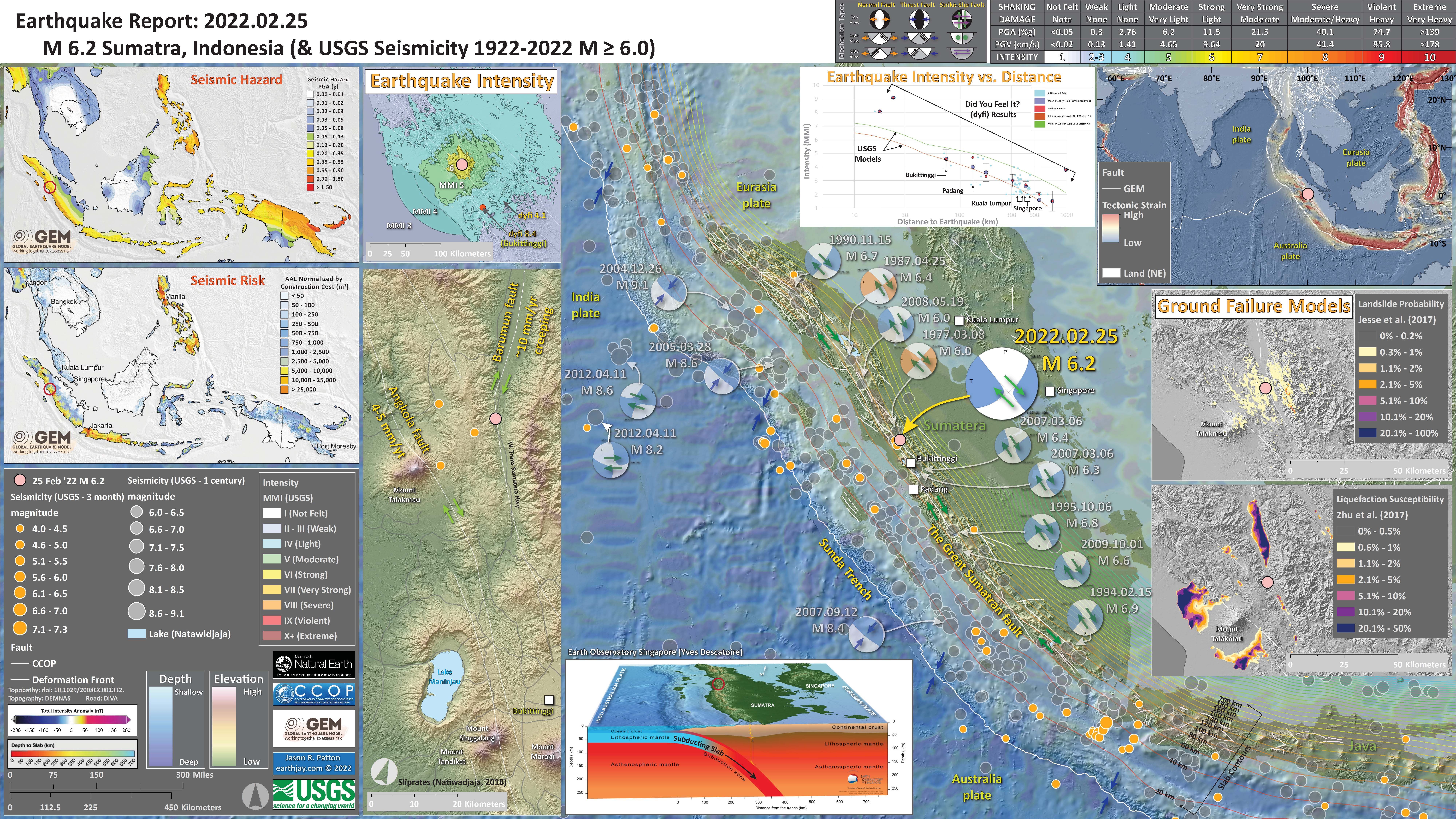
Below is my interpretive poster for this earthquake
- I plot the seismicity from the past 3 months, with diameter representing magnitude (see legend). I include earthquake epicenters from 1922-2022 with magnitudes M ≥ 6.0.
- I plot the USGS fault plane solutions (moment tensors in blue and focal mechanisms in orange), possibly in addition to some relevant historic earthquakes.
- A review of the basic base map variations and data that I use for the interpretive posters can be found on the Earthquake Reports page. I have improved these posters over time and some of this background information applies to the older posters.
- Some basic fundamentals of earthquake geology and plate tectonics can be found on the Earthquake Plate Tectonic Fundamentals page.
- In the upper right corner is a map that shows the major plate boundaries with tectonic strain shown in red and blue. Areas that are red have a higher rate of tectonic deformation due to the motion of these plates and the orientation of the plate boundaries.
- In the lower center is a low angle oblique view of the Sumatra subduction zone that forms the Sunda Trench. I placed a red circle in the location of the M 6.2 earthquake.
- In the upper left center there is a map that shows the earthquake shaking intensity. Read more about this further down in this report.
- In the upper right center is a plot showing earthquake shaking intensity (vertical axis) relative to distance from the earthquake (horizontal axis). This shows a comparison between the USGS shaking models as colored lines (also shown on the map to the left) relative to real reports from real people (the Did You Feel It? (dyfi) points).
- Below the earthquake intensity map is a map that shows the mapped active faults, along with their slip rates from Natawidjaja (2018).
- On the right margin are two maps that show models of earthquake triggered landslides and earthquake induced liquefaction. I describe these phenomena later in this report.
- In the upper left corner are two maps from the Global Earthquake Model program: Seismic Hazard and Seismic Risk. Read more about this later in this report.
I include some inset figures. Some of the same figures are located in different places on the larger scale map below.
- Here is the map with 3 month’s seismicity plotted.
Some Relevant Discussion and Figures
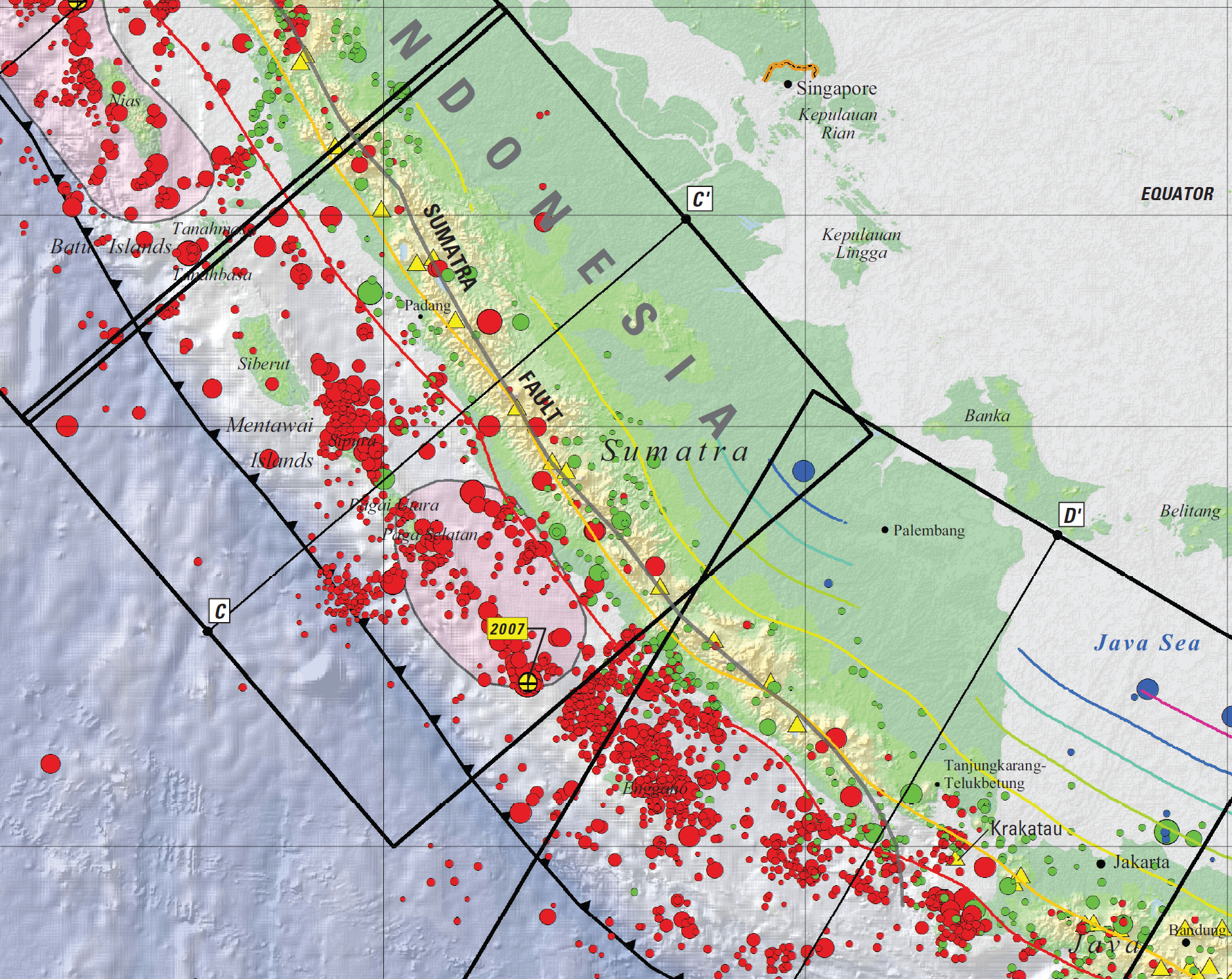
- Here is a part of the poster “Seismicity of the Earth 1900-2012, Sumatra and Vicinity” (Hayes et al., 2013). Note the location of Padang, which is southwest of the M 6.2 earthquake.
- The map shows the location of the seismicity cross section (the next figure). The cross section includes earthquakes from locations within the rectangle. These events are plotted along the line C-C.’
- See that the Sumatra fault crosses this cross section just to the east of the center.
- Here is the seismicity cross section C-C’. Many of the earthquakes plotted here follow the subducting slab of the India-Australia plate.
- However, there are some shallow earthquakes in the upper plate that represent slip along Sumatra fault zone faults (like yesterday’s M 6.2).
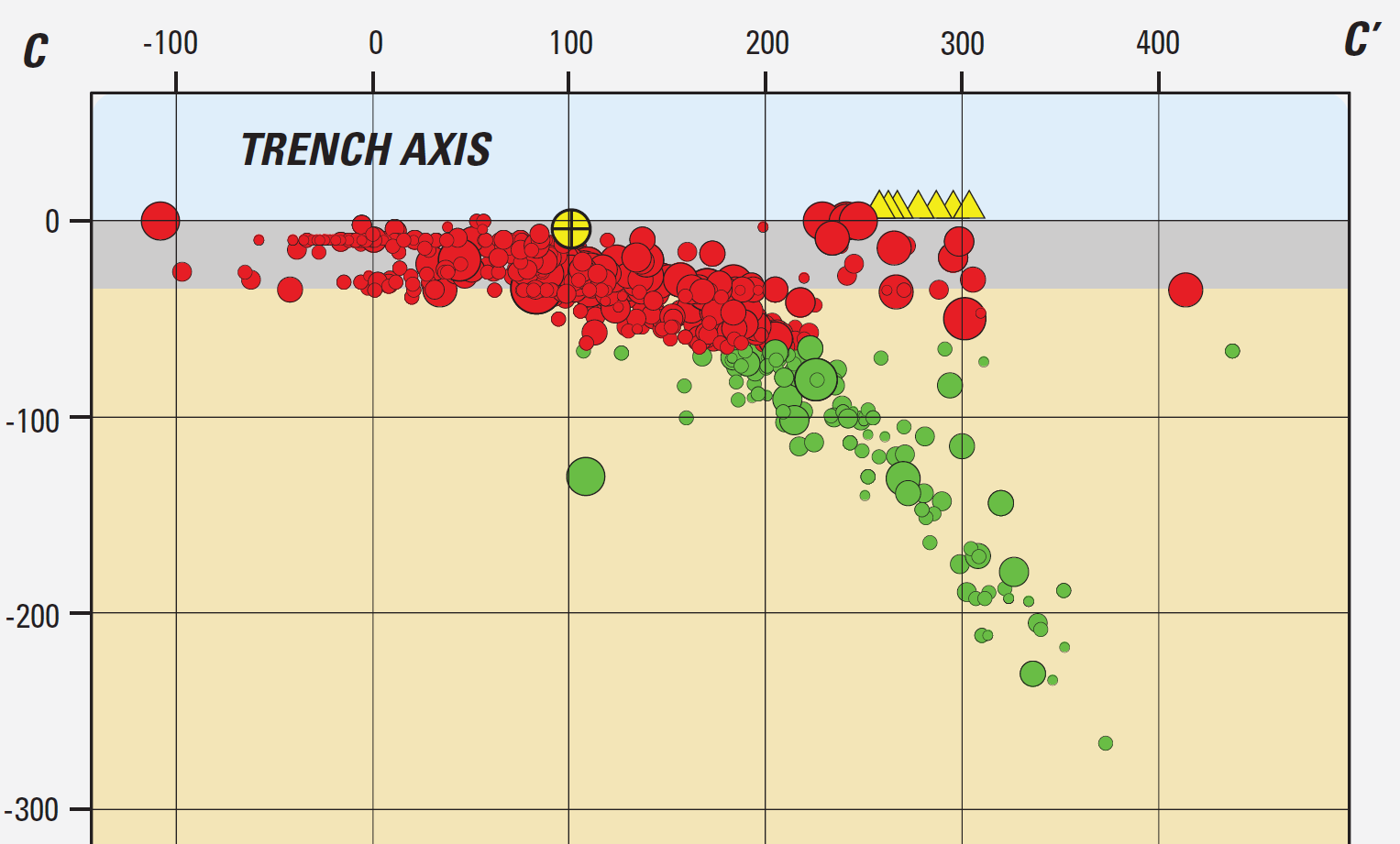
- Further to the north there was a pair of subduction zone earthquakes in 2004 and 2005. The 2004 Sumatra-Andaman subduction zone earthquake was devastating and the earthquake and tsunami led to almost a quarter of million deaths.
- There are several earthquake report pages on these two events. Here is one of them:/li>
- M 9.2 Andaman-Sumatra subduction zone 2016 Earthquake Anniversary
- This is my poster from that report.
- Here is a cross section showing where the earthquake hypocenter is compared to where we think the mantle exists. We have not been here, so nobody actually knows… These interpretations are based on industry deep seismic data (Singh et al., 2008 ).
- Here is the historic rupture map showing the locations of historic subduction zone earthquakes. I include a figure caption below that I wrote as blockquote.

India-Australia plate subducts northeastwardly beneath the Sunda plate (part of Eurasia) at modern rates (GPS velocities are based on regional modeling of Bock et al, 2003 as plotted in Subarya et al., 2006). Historic earthquake ruptures (Bilham, 2005; Malik et al., 2011) are plotted in orange. 2004 earthquake and 2005 earthquake 5 meter slip contours are plotted in orange and green respectively (Chlieh et al., 2007, 2008). Bengal and Nicobar fans cover structures of the India-Australia plate in the northern part of the map. RR0705 cores are plotted as light blue. SRTM bathymetry and topography is in shaded relief and colored vs. depth/elevation (Smith and Sandwell, 1997).
- One of my favorite interpretive posters for this part of the world is from the 2012 outer rise sequence offshore of northern Sumatra. This poster includes additional details about the structure of the India-Australia plate.
- The India-Australia plate is important as it appears to control some of the tectonics of the megathrust, as well as for the upper plate faults like the Sumatra fault.
- Read more about the 2012 sequence here.

- This is a video showing a visualization of the seismic waves transmitted from the 2004 SASZ earthquake from IRIS and others.
This movie illustrates simulation of seismic wave propagation generated by Dec. 26 Sumatra earthquake. Colors indicate amplitude of vertical displacement at the surface of the Earth. Red is upward and blue is downward. Total duration of this simulation is 20 minutes. Source model we used is that of Chen Ji of Caltech. Simulation was performed by using the Earth Simulator of JAMSTEC.
- Here is a great figure from Philobosian et al. (2014) that shows the slip patches from the subduction zone earthquakes in this region.

Map of Southeast Asia showing recent and selected historical ruptures of the Sunda megathrust. Black lines with sense of motion are major plate-bounding faults, and gray lines are seafloor fracture zones. Motions of Australian and Indian plates relative to Sunda plate are from the MORVEL-1 global model [DeMets et al., 2010]. The fore-arc sliver between the Sunda megathrust and the strike-slip Sumatran Fault becomes the Burma microplate farther north, but this long, thin strip of crust does not necessarily all behave as a rigid block. Sim = Simeulue, Ni = Nias, Bt = Batu Islands, and Eng = Enggano. Brown rectangle centered at 2°S, 99°E delineates the area of Figure 3, highlighting the Mentawai Islands. Figure adapted from Meltzner et al. [2012] with rupture areas and magnitudes from Briggs et al. [2006], Konca et al. [2008], Meltzner et al. [2010], Hill et al. [2012], and references therein.
- Now let’s take a closer look at the Sumatra fault. Here is a map that is from Natawidjaja (2017). Dr. Natawidjaja worked with Dr. Kerry Sieh on the Sumatra fault for his Ph.D. research. This map is an updated version showing the different fault segments of the Sumatra fault system. I inlcude their figure caption in blackquote.
- Here is a figure from their dissertation showing these fault segments in greater detail (Natawidjaja , 2002). The M 6.2 earthquake is near the southern boundary of the Barumun segment.
- This map shows what the slip rate would be on an hypothetical forearc sliver fault in the location of the Sumatra fault, given plate convergence rates and coral uplift rates (Natawidjaja, 2017).
- This figure shows a comparison of fault slip rates for different parts of the Sumatra fault (Natawidjaja, 2017).
- And finally here is an interpretive figure showing how Natawidjaja(2002) interpret the formation of the Sumatra fault system.
New revised (simplified) active fault map of the Sumatran Fault Zone (SFZ) according to the PuSGeN Team for Updating Indonesia Seismic Hazard Map (2016) with new slip rates from geological and geodetical (GPS) recent studies.
Map of 20 geometrically defined segments of the Sumatran fault system and their spatial relationships to active volcanoes, major graben, and lakes.
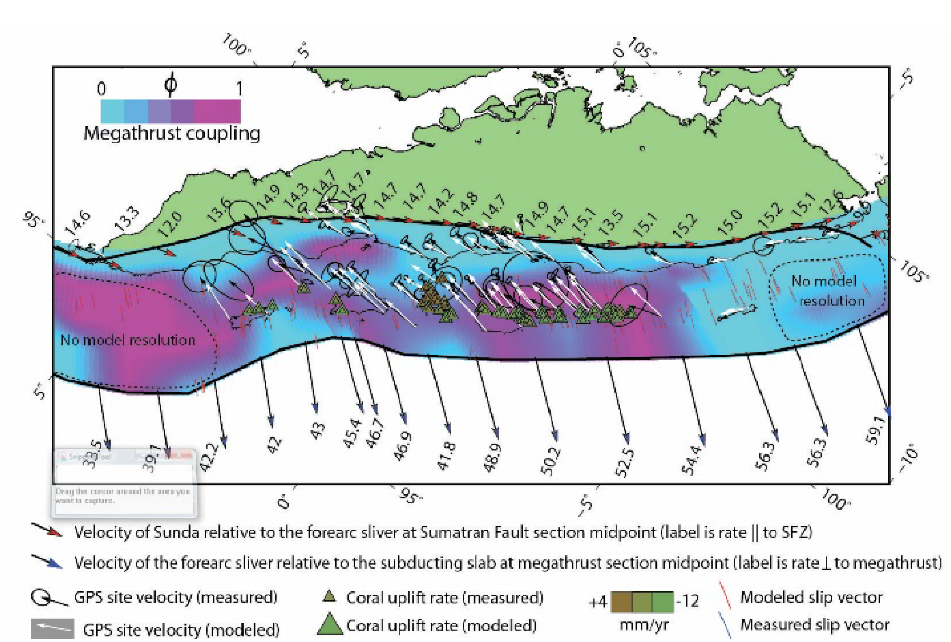
Tectonic modelling based on continuous GPS – SuGAr 9 Sumatran GPS Array) and coral uplift rates,
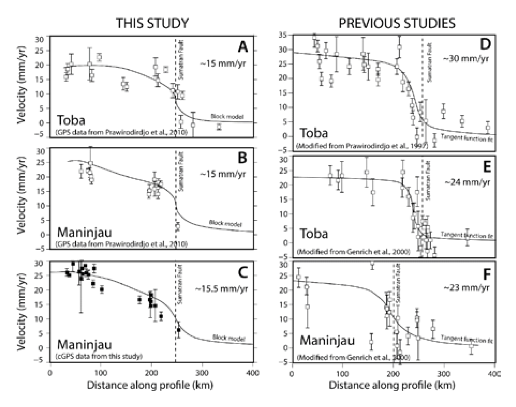
Comparison of GPS velocity profiles across the Sumatran fore arc inferred from (left) kinematic block models (right) with previously published velocity profiles. Modeling all fore-arc site velocities with a single strike-slip fault results in anomalously high inferred slip-rates (>22mm/yr) and missing the Sumatran Fault trace by up to 40km. Incorporating the effect of oblique locking of the Sunda megathrust results in lower inferred slip – rates for the Sumatran Fault (~15mm/yr) that are more consistent with updated geological slip rates.
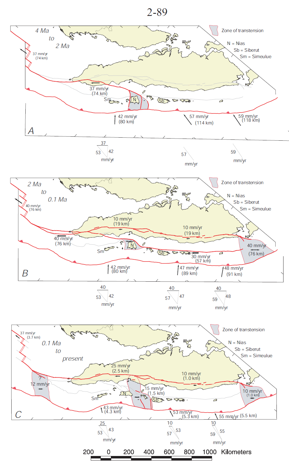
A plausible (but nonunique) history of deformation along the obliquely convergent Sumatran plate margin, based upon our work and consistent with GPS results and the timing of deformation in the forearc region. (a) By about 4 Ma, the outer-arc ridge has formed. The former deformation front and the Mentawai homocline provide a set of reference features for assessing later deformations. From 4 to 2 Ma, partitioning of oblique plate convergence occurs only north of the equator. Dextral-slip faults on the northeast flank of the forearc sliver plate parallel the trench in northern Sumatra but swing south and disarticulate the forearc basin and outer-arc ridge north of the equator. (b) Slip partitioning begins south of the equator about 2 Ma, with the creation of the Mentawai and Sumatran faults. Transtension continues in the forearc north of the equator. (c) In perhaps just the past 100 yr, the Mentawai fault has become inactive, and the rate of slip on the Sumatran fault north of 2°N has more than doubled. This difference in slip rate may be accommodated by a new zone of transtension between the Sumatran fault and the deformation front in the forearc and outer-arc regions.
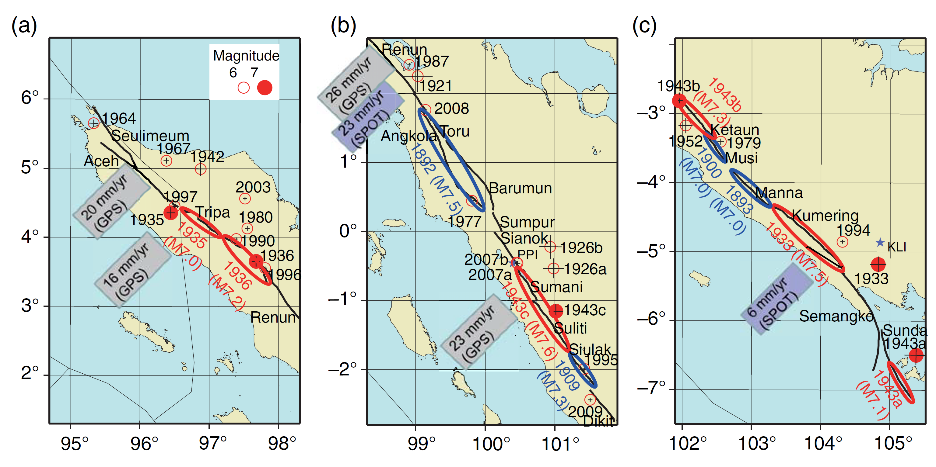
Relocated MJHD epicenters. (a) Northern Sumatra. (b) Central Sumatra. (c) Southern Sumatra. Solid lines with names indicate segments of the Sumatran fault (Sieh and Natawidjaja, 2000). Symbols are as in Figure 2. The thick solid line (see Fig. 4c) indicates the Ranau–Suwoh area, which was severely damaged by the 1933 Liwa earthquake (Berlage, 1934;Widiwijayanti et al., 1996). The slip rates of the Sumatran fault in northern, central, and southern Sumatra are taken from Ito et al. (2012) and Genrich et al. (2000) for Global Positioning System (GPS) and Bellier and Sebrier (1995) for Satellite Pour l’Observation de la Terre (SPOT).
Earthquake history along the Sumatran fault since 1892. Fault planes estimated in this study are shown by thick lines. SG: Seismic gap.
Earthquake Stress Triggering
- When an earthquake fault slips, the crust surrounding the fault squishes and expands, deforming elastically (like in one’s underwear). These changes in shape of the crust cause earthquake fault stresses to change. These changes in stress can either increase or decrease the chance of another earthquake.
- I wrote more about this type of earthquake triggering for Temblor here. Head over there to learn more about “static coulomb stress triggering.”
- There are two kinds of earthquake triggering.
- Dynamic Triggering – When seismic waves travel through the Earth, they change the stresses in the crust. IF the faults are “locked and loaded” (i.e. they are just about ready to slip in an earthquake), there may be an earthquake on the “receiver” fault. Generally, once the seismic waves are done travelling, this effect is over. Though, some suggest that this affect on the stress changes may last longer (but not much longer).
- Static Triggering – When an earthquake fault slips, it deforms (changes the shape) of the crust surrounding that earthquake. These changes can cause increases and decreases in the stress on faults (either increasing or decreasing the chance for an earthquake). Just like for dynamic triggering, the fault needs to be about ready to slip. The effect on fault slip changes in “static coulomb stress” generally extend a distance of about 2-3 times the fault length of the “source” fault.
- Raffie et al. (2021) calculated static coulomb stress changes on the central Sumatra fault segments as imposed by several megathrust subduction zone earthquakes.
- Below is a series of maps that show the results from their analyses.
- Here are the results when they consider all sources in a cumulative manner.

Coulomb stress models resolved on receiver faults of central part of GSF from coseismic slip model of each large interplate earthquakes. The color represents the maximum stress changes at 10 km depth with a scale saturated at 1 bar.
Cumulative ΔCFF of each earthquake listed in Table 1 (a) and cumulative ΔCFF of 1797, 1833, and 1861 earthquakes (b). The cyan ellipses are the damage area of large intraplate earthquakes marked as green star. The ΔCFF is calculated at 10 km depth with a scale saturated at 1 bar.
Shaking Intensity
- Here is a figure that shows a more detailed comparison between the modeled intensity and the reported intensity. Both data use the same color scale, the Modified Mercalli Intensity Scale (MMI). More about this can be found here. The colors and contours on the map are results from the USGS modeled intensity. The DYFI data are plotted as colored dots (color = MMI, diameter = number of reports).
- In the upper panel is the USGS Did You Feel It reports map, showing reports as colored dots using the MMI color scale. Underlain on this map are colored areas showing the USGS modeled estimate for shaking intensity (MMI scale).
- In the lower panel is a plot showing MMI intensity (vertical axis) relative to distance from the earthquake (horizontal axis). The models are represented by the green and orange lines. The DYFI data are plotted as light blue dots. The mean and median (different types of “average”) are plotted as orange and purple dots. Note how well the reports fit the green line (the model that represents how MMI works based on quakes in California).
- Below the lower plot is the USGS MMI Intensity scale, which lists the level of damage for each level of intensity, along with approximate measures of how strongly the ground shakes at these intensities, showing levels in acceleration (Peak Ground Acceleration, PGA) and velocity (Peak Ground Velocity, PGV).

Potential for Ground Failure
- Below are a series of maps that show the potential for landslides and liquefaction. These are all USGS data products.
There are many different ways in which a landslide can be triggered. The first order relations behind slope failure (landslides) is that the “resisting” forces that are preventing slope failure (e.g. the strength of the bedrock or soil) are overcome by the “driving” forces that are pushing this land downwards (e.g. gravity). The ratio of resisting forces to driving forces is called the Factor of Safety (FOS). We can write this ratio like this:FOS = Resisting Force / Driving Force
- When FOS > 1, the slope is stable and when FOS < 1, the slope fails and we get a landslide. The illustration below shows these relations. Note how the slope angle α can take part in this ratio (the steeper the slope, the greater impact of the mass of the slope can contribute to driving forces). The real world is more complicated than the simplified illustration below.
- Landslide ground shaking can change the Factor of Safety in several ways that might increase the driving force or decrease the resisting force. Keefer (1984) studied a global data set of earthquake triggered landslides and found that larger earthquakes trigger larger and more numerous landslides across a larger area than do smaller earthquakes. Earthquakes can cause landslides because the seismic waves can cause the driving force to increase (the earthquake motions can “push” the land downwards), leading to a landslide. In addition, ground shaking can change the strength of these earth materials (a form of resisting force) with a process called liquefaction.
- Sediment or soil strength is based upon the ability for sediment particles to push against each other without moving. This is a combination of friction and the forces exerted between these particles. This is loosely what we call the “angle of internal friction.” Liquefaction is a process by which pore pressure increases cause water to push out against the sediment particles so that they are no longer touching.
- An analogy that some may be familiar with relates to a visit to the beach. When one is walking on the wet sand near the shoreline, the sand may hold the weight of our body generally pretty well. However, if we stop and vibrate our feet back and forth, this causes pore pressure to increase and we sink into the sand as the sand liquefies. Or, at least our feet sink into the sand.
- Below is a diagram showing how an increase in pore pressure can push against the sediment particles so that they are not touching any more. This allows the particles to move around and this is why our feet sink in the sand in the analogy above. This is also what changes the strength of earth materials such that a landslide can be triggered.
- Below is a diagram based upon a publication designed to educate the public about landslides and the processes that trigger them (USGS, 2004). Additional background information about landslide types can be found in Highland et al. (2008). There was a variety of landslide types that can be observed surrounding the earthquake region. So, this illustration can help people when they observing the landscape response to the earthquake whether they are using aerial imagery, photos in newspaper or website articles, or videos on social media. Will you be able to locate a landslide scarp or the toe of a landslide? This figure shows a rotational landslide, one where the land rotates along a curvilinear failure surface.
- Below is the liquefaction susceptibility and landslide probability map (Jessee et al., 2017; Zhu et al., 2017). Please head over to that report for more information about the USGS Ground Failure products (landslides and liquefaction). Basically, earthquakes shake the ground and this ground shaking can cause landslides.
- I use the same color scheme that the USGS uses on their website. Note how the areas that are more likely to have experienced earthquake induced liquefaction are in the valleys. Learn more about how the USGS prepares these model results here.


Seismic Hazard and Seismic Risk
- Here is a map that shows the seismic hazard in southeast Asia, including Sumatra (Hayes et al., 2013). The plate convergence vectors, showing the direction of plate convergence and the rate of plate convergence in mm per year. Note how the plate convergence vectors are not perpendicular to the plate boundary.

- These are the two maps shown in the map above, the GEM Seismic Hazard and the GEM Seismic Risk maps from Pagani et al. (2018) and Silva et al. (2018).
- The GEM Seismic Hazard Map:
- The Global Earthquake Model (GEM) Global Seismic Hazard Map (version 2018.1) depicts the geographic distribution of the Peak Ground Acceleration (PGA) with a 10% probability of being exceeded in 50 years, computed for reference rock conditions (shear wave velocity, VS30, of 760-800 m/s). The map was created by collating maps computed using national and regional probabilistic seismic hazard models developed by various institutions and projects, and by GEM Foundation scientists. The OpenQuake engine, an open-source seismic hazard and risk calculation software developed principally by the GEM Foundation, was used to calculate the hazard values. A smoothing methodology was applied to homogenise hazard values along the model borders. The map is based on a database of hazard models described using the OpenQuake engine data format (NRML). Due to possible model limitations, regions portrayed with low hazard may still experience potentially damaging earthquakes.
- Here is a view of the GEM seismic hazard map for Indonesia.
- The GEM Seismic Risk Map:
- The Global Seismic Risk Map (v2018.1) presents the geographic distribution of average annual loss (USD) normalised by the average construction costs of the respective country (USD/m2) due to ground shaking in the residential, commercial and industrial building stock, considering contents, structural and non-structural components. The normalised metric allows a direct comparison of the risk between countries with widely different construction costs. It does not consider the effects of tsunamis, liquefaction, landslides, and fires following earthquakes. The loss estimates are from direct physical damage to buildings due to shaking, and thus damage to infrastructure or indirect losses due to business interruption are not included. The average annual losses are presented on a hexagonal grid, with a spacing of 0.30 x 0.34 decimal degrees (approximately 1,000 km2 at the equator). The average annual losses were computed using the event-based calculator of the OpenQuake engine, an open-source software for seismic hazard and risk analysis developed by the GEM Foundation. The seismic hazard, exposure and vulnerability models employed in these calculations were provided by national institutions, or developed within the scope of regional programs or bilateral collaborations.
- Here is a view of the GEM seismic risk map for Indonesia.

Tsunami Hazard
- Here are two maps that show the results of probabilistic tsunami modeling for the nation of Indonesia (Horspool et al., 2014). These results are similar to results from seismic hazards analysis and maps. The color represents the chance that a given area will experience a certain size tsunami (or larger).
- The first map shows the annual chance of a tsunami with a height of at least 0.5 m (1.5 feet). The second map shows the chance that there will be a tsunami at least 3 meters (10 feet) high at the coast.
Annual probability of experiencing a tsunami with a height at the coast of (a) 0.5m (a tsunami warning) and (b) 3m (a major tsunami warning).
- M 9.2 Andaman-Sumatra subduction zone 2014 Earthquake Anniversary
- M 9.2 Andaman-Sumatra subduction zone SASZ Fault Deformation
- M 9.2 Andaman-Sumatra subduction zone 2016 Earthquake Anniversary
- 2022.02.25 M 6.2 Sumatra
- 2020.05.06 M 6.8 Banda Sea
- 2019.08.02 M 6.9 Indonesia
- 2019.06.23 M 7.3 Banda Sea
- 2019.04.12 M 6.8 Sulawesi, Indonesia
- 2018.09.28 M 7.5 Sulawesi
- 2018.10.16 M 7.5 Sulawesi UPDATE #1
- 2018.08.19 M 6.9 Lombok, Indonesia
- 2018.08.05 M 6.9 Lombok, Indonesia
- 2018.07.28 M 6.4 Lombok, Indonesia
- 2017.12.15 M 6.5 Java
- 2017.08.31 M 6.3 Mentawai, Sumatra
- 2017.08.13 M 6.4 Bengkulu, Sumatra, Indonesia
- 2017.05.29 M 6.8 Sulawesi, Indonesia
- 2017.03.14 M 6.0 Sumatra
- 2017.03.01 M 5.5 Banda Sea
- 2016.10.19 M 6.6 Java
- 2016.03.02 M 7.8 Sumatra/Indian Ocean
- 2015.07.22 M 5.8 Andaman Sea
- 2015.11.08 M 6.4 Nicobar Isles
- 2012.04.11 M 8.6 Sumatra outer rise
- 2004.12.26 M 9.2 Andaman-Sumatra subduction zone
Indonesia | Sumatra
General Overview
Earthquake Reports
Social Media
#EarthquakeReport for M 6.2 #Gempa #Earthquake along the #Sumatra fault just north of #Padang
evidence for strong ground shaking and possible surface rupture
historical analogueshttps://t.co/Se0jsMEvGOread more herehttps://t.co/xujTF3MERq pic.twitter.com/tWEhQTCj06
— Jason "Jay" R. Patton (@patton_cascadia) February 27, 2022
A Mw6.2 earthquake just occurred along the Sumatran Fault in Indonesia.
This fault extends for >1700 km, slicing Sumatra in two. The fault aligns closely with the volcanoes generated by the subduction zone to the west. See the fault & volcanoes in the topography below!
🧵 1/ https://t.co/rY6yzEwBwG pic.twitter.com/5gd5YjaPfG
— Dr. Judith Hubbard (@JudithGeology) February 25, 2022
Kondisi saat ini di Kec. Talamau Pasaman Barat. Bagi manteman yang ada dilokasi boleh mention kondisi di sana ya @infomitigasi @JogjaUpdate pic.twitter.com/910vTLMioM
— Podcast Asap_id (@podcastasap_id) February 25, 2022
An earthquake with Mw 6.2 struck inland with dextral mechanism in the segmentation of Sumatra Fault on this morning (Indonesia Time), killing at least two people and causing tremors that were felt until Singapore and Malaysia. pic.twitter.com/Gd8MoXC8u4
— andrean (@andreanjtk) February 25, 2022
Rangkaian #Gempa yang terjadi di #Sumbar, tapatnya di #Pasamanbarat pada 25 Feb 2022. Rangkaian gempa ini diawal oleh gempa pembuka (foreshock) M=5,2 (08:35:51 WIB), berselang 3 menit 42 detik diikuti oleh gempa utama M=6,2 (08:39:29 WIB). pic.twitter.com/iNQL9tiIcZ
— Zulfakriza Z. (@zulfakriza) February 25, 2022
Akibat Gempa di Pasbar terjadi juga longsor di Malampah Pasaman pic.twitter.com/WU9MJ7pSFm
— Yazid Lubis (@YazidLubis9) February 25, 2022
Did you feel shaking from this morning's #Sumatra earthquake? The rupture occured along a segment of the Sumatran Fault. While the segment is 400km away from #Singapore, it was widely felt across the island. Learn more about today's event in our blog post https://t.co/bY8KDv3GAx
— Earth Observatory SG (@EOS_SG) February 25, 2022
6.1 Mw North-Central Sumatra (#INDONESIA 🇮🇩), a right-lateral strike-slip "Southern Angkola Segment" (Great Sumatran Fault System), potentially for a >7.5 Mw. pic.twitter.com/YSXqgH1Ge1
— Abel Seism🌏Sánchez (@EQuake_Analysis) February 25, 2022
Some hours ago, strong shallow M6.2 #earthquake in Sumatra, widely felt also in Malaysia and Singapore.
Hope everybody is OK in the epicentral area.https://t.co/0cddTk78dK pic.twitter.com/MW9G6IwTje— José R. Ribeiro (@JoseRodRibeiro) February 25, 2022
Di dekat episenter gempa Pasaman Mag. 6,1 tadi pagi, pada bulan Januari 2022 sudah terjadi 2 gempa tidak dirasakan. pic.twitter.com/IWQvwvAlVY
— DARYONO BMKG (@DaryonoBMKG) February 25, 2022
Pasca Gempa di Pasaman Barat semburkan air panas di Bonjol Sumatera Barat.
Padang Gempa Sumbar pic.twitter.com/cBBQka8hkj— David Haris St Parmato (@DavidHaris10) February 25, 2022
Ground failure pasca gempa kuat. https://t.co/2ApLwk83aq
— DARYONO BMKG (@DaryonoBMKG) February 25, 2022
Vibrasi periode panjang terjadi di Malaysia saat gempa M6,1 Pasaman. https://t.co/zCegE51eI9
— DARYONO BMKG (@DaryonoBMKG) February 25, 2022
- Frisch, W., Meschede, M., Blakey, R., 2011. Plate Tectonics, Springer-Verlag, London, 213 pp.
- Hayes, G., 2018, Slab2 – A Comprehensive Subduction Zone Geometry Model: U.S. Geological Survey data release, https://doi.org/10.5066/F7PV6JNV.
- Holt, W. E., C. Kreemer, A. J. Haines, L. Estey, C. Meertens, G. Blewitt, and D. Lavallee (2005), Project helps constrain continental dynamics and seismic hazards, Eos Trans. AGU, 86(41), 383–387, , https://doi.org/10.1029/2005EO410002. /li>
- Jessee, M.A.N., Hamburger, M. W., Allstadt, K., Wald, D. J., Robeson, S. M., Tanyas, H., et al. (2018). A global empirical model for near-real-time assessment of seismically induced landslides. Journal of Geophysical Research: Earth Surface, 123, 1835–1859. https://doi.org/10.1029/2017JF004494
- Kreemer, C., J. Haines, W. Holt, G. Blewitt, and D. Lavallee (2000), On the determination of a global strain rate model, Geophys. J. Int., 52(10), 765–770.
- Kreemer, C., W. E. Holt, and A. J. Haines (2003), An integrated global model of present-day plate motions and plate boundary deformation, Geophys. J. Int., 154(1), 8–34, , https://doi.org/10.1046/j.1365-246X.2003.01917.x.
- Kreemer, C., G. Blewitt, E.C. Klein, 2014. A geodetic plate motion and Global Strain Rate Model in Geochemistry, Geophysics, Geosystems, v. 15, p. 3849-3889, https://doi.org/10.1002/2014GC005407.
- Meyer, B., Saltus, R., Chulliat, a., 2017. EMAG2: Earth Magnetic Anomaly Grid (2-arc-minute resolution) Version 3. National Centers for Environmental Information, NOAA. Model. https://doi.org/10.7289/V5H70CVX
- Müller, R.D., Sdrolias, M., Gaina, C. and Roest, W.R., 2008, Age spreading rates and spreading asymmetry of the world’s ocean crust in Geochemistry, Geophysics, Geosystems, 9, Q04006, https://doi.org/10.1029/2007GC001743
- Pagani,M. , J. Garcia-Pelaez, R. Gee, K. Johnson, V. Poggi, R. Styron, G. Weatherill, M. Simionato, D. Viganò, L. Danciu, D. Monelli (2018). Global Earthquake Model (GEM) Seismic Hazard Map (version 2018.1 – December 2018), DOI: 10.13117/GEM-GLOBAL-SEISMIC-HAZARD-MAP-2018.1
- Silva, V ., D Amo-Oduro, A Calderon, J Dabbeek, V Despotaki, L Martins, A Rao, M Simionato, D Viganò, C Yepes, A Acevedo, N Horspool, H Crowley, K Jaiswal, M Journeay, M Pittore, 2018. Global Earthquake Model (GEM) Seismic Risk Map (version 2018.1). https://doi.org/10.13117/GEM-GLOBAL-SEISMIC-RISK-MAP-2018.1
- Zhu, J., Baise, L. G., Thompson, E. M., 2017, An Updated Geospatial Liquefaction Model for Global Application, Bulletin of the Seismological Society of America, 107, p 1365-1385, https://doi.org/0.1785/0120160198
- Abercrombie, R.E., Antolik, M., Ekstrom, G., 2003. The June 2000 Mw 7.9 earthquakes south of Sumatra: Deformation in the India–Australia Plate. Journal of Geophysical Research 108, 16.
- Bassin, C., Laske, G. and Masters, G., The Current Limits of Resolution for Surface Wave Tomography in North America, EOS Trans AGU, 81, F897, 2000.
- Bock, Y., Prawirodirdjo, L., Genrich, J.F., Stevens, C.W., McCaffrey, R., Subarya, C., Puntodewo, S.S.O., Calais, E., 2003. Crustal motion in Indonesia from Global Positioning System measurements: Journal of Geophysical Research, v. 108, no. B8, 2367, doi: 10.1029/2001JB000324.
- Bothara, J., Beetham, R.D., Brunston, D., Stannard, M., Brown, R., Hyland, C., Lewis, W., Miller, S., Sanders, R., Sulistio, Y., 2010. General observations of effects of the 30th September 2009 Padang earthquake, Indonesia. Bulletin of the New Zealand Society for Earthquake Engineering 43, 143-173.
- Chlieh, M., Avouac, J.-P., Hjorleifsdottir, V., Song, T.-R.A., Ji, C., Sieh, K., Sladen, A., Hebert, H., Prawirodirdjo, L., Bock, Y., Galetzka, J., 2007. Coseismic Slip and Afterslip of the Great (Mw 9.15) Sumatra-Andaman Earthquake of 2004. Bulletin of the Seismological Society of America 97, S152-S173.
- Chlieh, M., Avouac, J.P., Sieh, K., Natawidjaja, D.H., Galetzka, J., 2008. Heterogeneous coupling of the Sumatran megathrust constrained by geodetic and paleogeodetic measurements: Journal of Geophysical Research, v. 113, B05305, doi: 10.1029/2007JB004981.
- DEPLUS, C. et al., 1998 – Direct evidence of active derormation in the eastern Indian oceanic plate, Geology.
- DYMENT, J., CANDE, S.C. & SINGH, S., 2007 – Oceanic lithosphere subducting beneath the Sunda Trench: the Wharton Basin revisited. European Geosciences Union General Assembly, Vienna, 15-20/05.
- Hayes, G. P., Wald, D. J., and Johnson, R. L., 2012. Slab1.0: A three-dimensional model of global subduction zone geometries in J. Geophys. Res., 117, B01302, doi:10.1029/2011JB008524.
- Hayes, G.P., Bernardino, Melissa, Dannemann, Fransiska, Smoczyk, Gregory, Briggs, Richard, Benz, H.M., Furlong, K.P., and Villaseñor, Antonio, 2013. Seismicity of the Earth 1900–2012 Sumatra and vicinity: U.S. Geological Survey Open-File Report 2010–1083-L, scale 1:6,000,000, https://pubs.usgs.gov/of/2010/1083/l/.
- JACOB, J., DYMENT, J., YATHEESH, V. & BHATTACHARYA, G.C., 2009 – Marine magnetic anomalies in the NE Indian Ocean: the Wharton and Central Indian basins revisited. European Geosciences Union General Assembly, Vienna, 19-24/04.
- Ji, C., D.J. Wald, and D.V. Helmberger, Source description of the 1999 Hector Mine, California earthquake; Part I: Wavelet domain inversion theory and resolution analysis, Bull. Seism. Soc. Am., Vol 92, No. 4. pp. 1192-1207, 2002.
- Hurukawa, N., Wulandari, B.R., and Kasahara, M., 2014. Earthquake History of the Sumatran Fault, Indonesia, since 1892, Derived from Relocation of Large Earthquakes in BSSA,v. 104, no. 4, p. 1750-1762, doi: 10.1785/0120130201
- Ishii, M., Shearer, P.M., Houston, H., Vidale, J.E., 2005. Extent, duration and speed of the 2004 Sumatra-Andaman earthquake imaged by the Hi-Net array. Nature 435, 933.
- Kanamori, H., Rivera, L., Lee, W.H.K., 2010. Historical seismograms for unravelling a mysterious earthquake: The 1907 Sumatra Earthquake. Geophysical Journal International 183, 358-374.
- Konca, A.O., Avouac, J., Sladen, A., Meltzner, A.J., Sieh, K., Fang, P., Li, Z., Galetzka, J., Genrich, J., Chlieh, M., Natawidjaja, D.H., Bock, Y., Fielding, E.J., Ji, C., Helmberger, D., 2008. Partial Rupture of a Locked Patch of the Sumatra Megathrust During the 2007 Earthquake Sequence. Nature 456, 631-635.
- Lange, D., Cembrano, J., Rietbrock, A., Haberland, C., Dahm, T., and Bataille, K., 2008. First seismic record for intra-arc strike-slip tectonics along the Liquiñe-Ofqui fault zone at the obliquely convergent plate margin of the southern Andes in Tectonophysics, v. 455, p. 14-24
- Maus, S., et al., 2009. EMAG2: A 2–arc min resolution Earth Magnetic Anomaly Grid compiled from satellite, airborne, and marine magnetic measurements, Geochem. Geophys. Geosyst., 10, Q08005, doi:10.1029/2009GC002471.
- Malik, J.N., Shishikura, M., Echigo, T., Ikeda, Y., Satake, K., Kayanne, H., Sawai, Y., Murty, C.V.R., Dikshit, D., 2011. Geologic evidence for two pre-2004 earthquakes during recent centuries near Port Blair, South Andaman Island, India: Geology, v. 39, p. 559-562.
- Meltzner, A.J., Sieh, K., Chiang, H., Shen, C., Suwargadi, B.W., Natawidjaja, D.H., Philobosian, B., Briggs, R.W., Galetzka, J., 2010. Coral evidence for earthquake recurrence and an A.D. 1390–1455 cluster at the south end of the 2004 Aceh–Andaman rupture. Journal of Geophysical Research 115, 1-46.
- Meng, L., Ampuero, J.-P., Stock, J., Duputel, Z., Luo, Y., and Tsai, V.C., 2012. Earthquake in a Maze: Compressional Rupture Branching During the 2012 Mw 8.6 Sumatra Earthquake in Science, v. 337, p. 724-726.
- Natawidjaja, D.H., Sieh, K., Chlieh, M., Galetzka, J., Suwargadi, B., Cheng, H., Edwards, R.L., Avouac, J., Ward, S.N., 2006. Source parameters of the great Sumatran megathrust earthquakes of 1797 and 1833 inferred from coral microatolls. Journal of Geophysical Research 111, 37.
- Natawidjaja, D.H., 2018. Updating active fault maps and slip rates along the Sumatran Fault Zone, Indonesia in IOP Conf. Ser.: Earth Environ. Sci. 118 012001
- Natawidjaja, D.H., 2002. Neotectonics of the Sumatran Fault And Paleogeodesy of the Sumatran Subduction Zone [thesis] Californiat Institute of Technilogy, Pasadena, California, 289 pp.
- Newcomb, K.R., McCann, W.R., 1987. Seismic History and Seismotectonics of the Sunda Arc. Journal of Geophysical Research 92, 421-439.
- Philibosian, B., Sieh, K., Natawidjaja, D.H., Chiang, H., Shen, C., Suwargadi, B., Hill, E.M., Edwards, R.L., 2012. An ancient shallow slip event on the Mentawai segment of the Sunda megathrust, Sumatra. Journal of Geophysical Research 117, 12.
- Prawirodirdjo, P., McCaffrey,R., Chadwell, D., Bock, Y, and Subarya, C., 2010. Geodetic observations of an earthquake cycle at the Sumatra subduction zone: Role of interseismic strain segmentation, JOURNAL OF GEOPHYSICAL RESEARCH, v. 115, B03414, doi:10.1029/2008JB006139
- Rafie, M.T., Cummins, P.R., Sahara, D.P., Widiyantoro, S., Triyoso, W., and Nugraha, A.D., 2021. Preliminary study of stress changes evolution on central part of Sumatran Fault influenced by large interplate earthquakes and tectonic stress rates, IOP Conf. Ser.: Earth Environ. Sci. 873 012011
- Rivera, L., Sieh, K., Helmberger, D., Natawidjaja, D.H., 2002. A Comparative Study of the Sumatran Subduction-Zone Earthquakes of 1935 and 1984. BSSA 92, 1721-1736.
- Shearer, P., and Burgmann, R., 2010. Lessons Learned from the 2004 Sumatra-Andaman Megathrust Rupture, Annu. Rev. Earth Planet. Sci. v. 38, pp. 103–31
- SATISH C. S, CARTON H, CHAUHAN A.S., et al., 2011 – Extremely thin crust in the Indian Ocean possibly resulting from Plume-Ridge Interaction, Geophysical Journal International.
- Sieh, K., Natawidjaja, D.H., Meltzner, A.J., Shen, C., Cheng, H., Li, K., Suwargadi, B.W., Galetzka, J., Philobosian, B., Edwards, R.L., 2008. Earthquake Supercycles Inferred from Sea-Level Changes Recorded in the Corals of West Sumatra. Science 322, 1674-1678.
- Singh, S.C., Carton, H.L., Tapponnier, P, Hananto, N.D., Chauhan, A.P.S., Hartoyo, D., Bayly, M., Moeljopranoto, S., Bunting, T., Christie, P., Lubis, H., and Martin, J., 2008. Seismic evidence for broken oceanic crust in the 2004 Sumatra earthquake epicentral region, Nature Geoscience, v. 1, pp. 5.
- Smith, W.H.F., Sandwell, D.T., 1997. Global seafloor topography from satellite altimetry and ship depth soundings: Science, v. 277, p. 1,957-1,962.
- Sorensen, M.B., Atakan, K., Pulido, N., 2007. Simulated Strong Ground Motions for the Great M 9.3 Sumatra–Andaman Earthquake of 26 December 2004. BSSA 97, S139-S151.
- Subarya, C., Chlieh, M., Prawirodirdjo, L., Avouac, J., Bock, Y., Sieh, K., Meltzner, A.J., Natawidjaja, D.H., McCaffrey, R., 2006. Plate-boundary deformation associated with the great Sumatra–Andaman earthquake: Nature, v. 440, p. 46-51.
- Tolstoy, M., Bohnenstiehl, D.R., 2006. Hydroacoustic contributions to understanding the December 26th 2004 great Sumatra–Andaman Earthquake. Survey of Geophysics 27, 633-646.
- Zhu, Lupei, and Donald V. Helmberger. “Advancement in source estimation techniques using broadband regional seismograms.” Bulletin of the Seismological Society of America 86.5 (1996): 1634-1641.
References:
Basic & General References
Specific References
Return to the Earthquake Reports page.
- Sorted by Magnitude
- Sorted by Year
- Sorted by Day of the Year
- Sorted By Region