This morning (my time) I was awakened by the tsunami notification that I get on my phone. I lept into action.
I get tsunami notifications so that I can respond to these potential tsunami events that may impact the coast of California as part of my job at the California Geological Survey.
There was a M 7.6 earthquake offshore of the island of Mindanao, Philippines. And, it was close to land (so a good chance that there may be casualties and damage).
I immediately thought of the people who live or visit there and what they must be experiencing. It is frightening to experience such a large magnitude earthquake.
https://earthquake.usgs.gov/earthquakes/eventpage/us7000lff4/executive
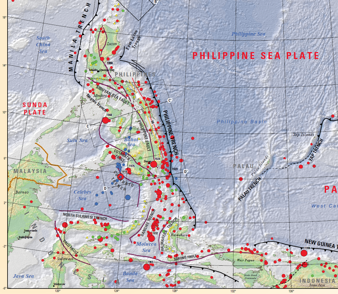
This part of the world is tectonically complicated. The nation of Philippines is bordered by convergent plate boundaries called subduction zones.
Subduction zones are where plates move towards each other. One of the plates dives down beneath the other plate. The interface of these plates is called the megathrust subduction zone earthquake fault.
To the east of the Philippines is the Philippines trench, a an area of very deep water formed by the subduction zone there where the Philippine Sea plate subducts beneath the Sunda plate (part of Eurasia). To the west is the Manila trench, where the Sunda plate subducts eastwards beneath the Philippine Sea plate.
Initially, it appeared that this earthquake may be a megathrust interface earthquake. However, the earthquake was too shallow to be on the subduction zone. The M 7.6 was actually somewhere in the upper plate.
However, there have been quite productive series of aftershocks and triggered earthquakes. Most of these earthquakes are not really aftershocks, since they are on different faults. The largest magnitude earthquakes, other than the M 7.6, appear related to the megathrust (e.g., the M 6.4 and M 6.9).
In fact, it appears that the M 7.6 has very few aftershocks. Most of the seismicity following the M 7.6 appear to be related to the megathrust triggered events.
Given the depth of the earthquake, if there was to be a tsunami, it would probably be a smaller one.
That is what came to be true. There is a tide gage near Davao City, in a location sheltered from a direct path from the M 7.4 epicenter (mapped location of the earthquake).
The tsunami is evident in these tide gage data. I plot these data below:
UPDATE: 4 Dec 2023
Above I write that the M 7.6 was likely on a thrust fault in the upper plate. This is based on the hypocentral (3-dimensional location of the earthquake) location relative to the USGS model of the subduction zone (“slab 2.0”).
We may think about “splay faults,” faults that begin at depth along the megathrust, but split off as separate faults and, possibly, reach the surface of the seafloor.
Dr. Judith Hubbard proposed an alternate hypothesis (see their tweet in the social media section below). The USGS slab 2.0 model may be too deep here. This is entirely possible, if not likely.
If Hubbard’s hypothesis is correct, it would place the abundance of the sequence on faults within the subducting plate.
This is also possible. However, I would have expected that the majority of these earthquakes would be along the megathrust, not within one of the plates.
Below is my interpretive poster for this earthquake
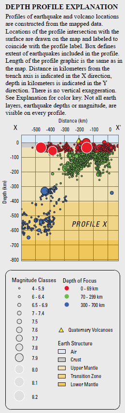
- I plot the seismicity from the past month, with diameter representing magnitude (see legend). I include earthquake epicenters from 1922-2022 with magnitudes M ≥ 3.0 in one version.
- I plot the USGS fault plane solutions (moment tensors in blue and focal mechanisms in orange), possibly in addition to some relevant historic earthquakes.
- A review of the basic base map variations and data that I use for the interpretive posters can be found on the Earthquake Reports page. I have improved these posters over time and some of this background information applies to the older posters.
- Some basic fundamentals of earthquake geology and plate tectonics can be found on the Earthquake Plate Tectonic Fundamentals page.
- In the upper left corner is a map showing the plate tectonic boundaries (from the GEM).
- Below the tectonic map is a low angle oblique view of the plate boundaries showing the subsurface geometry of the subduction zones (Hall, 2011). I placed an orange star in the location of the M 7.6.
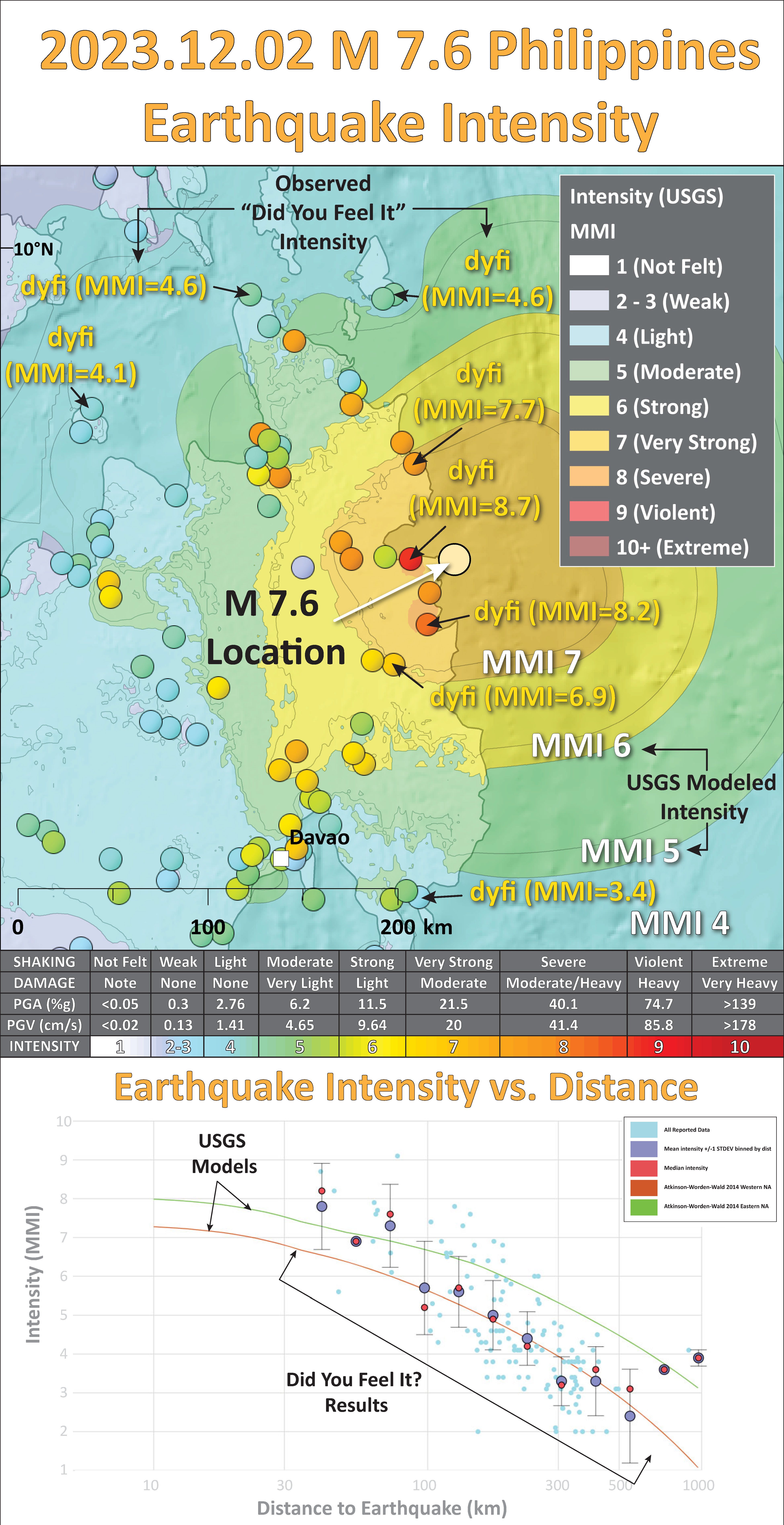
- In the lower right corner is a map that shows the M 7.4 earthquake intensity using the modified Mercalli intensity scale. Earthquake intensity is a measure of how strongly the Earth shakes during an earthquake, so gets smaller the further away one is from the earthquake epicenter. The map colors represent a model of what the intensity may be. The USGS has a system called “Did You Feel It?” (DYFI) where people enter their observations from the earthquake and the USGS calculates what the intensity was for that person. The dots with yellow labels show what people actually felt in those different locations.
- In the lower left center is a plot that shows the same intensity (both modeled and reported) data as displayed on the map. Note how the intensity gets smaller with distance from the earthquake.
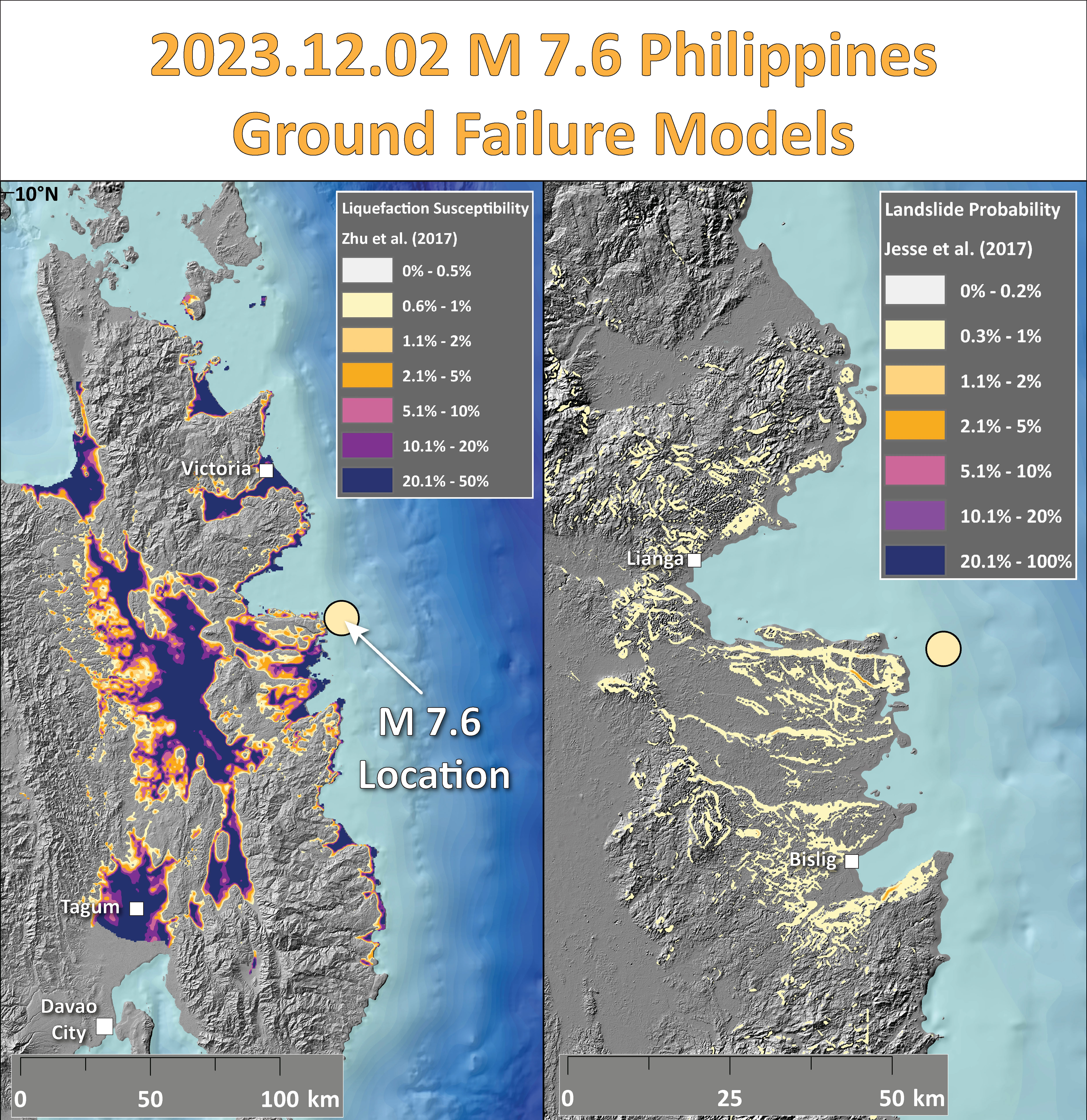
- In the upper right corner are two maps showing the possibility of earthquake induced liquefaction for these two earthquakes.
- To the left of the ground failure maps is a plot of the tide gage data from Davao.
- Above the intensity plot is the USGS fault slip model for this M 7.4 earthquake.
I include some inset figures. Some of the same figures are located in different places on the larger scale map below.
- Here is the map with a month’s seismicity plotted.
- Here is a map that shows a simplified version of the subduction zones in the region (Galgana et al., 2007).
- This is the low-angle oblique view of the region (Hall, 2011).
- This is smaller scale tectonic map of the region (Zahirovic et al., 2014).
- This is a map and series of cross sections showing subducting plates in blue (Zahirovic et al., 2014). The cross sections are based upon seismic wave tomography, which is similar to CT scans (Computed Tomography of X-Rays). These two processes use the same general methods to investigate the 3-dimensional views of internal structures (bodies vs. the Earth). More can be found in their paper, but basically, the blue regions represent areas that have higher seismic velocity. Oceanic lithosphere has higher seismic velocities than the surrounding mantle. So, the subducting oceanic slabs show up as blue. The corss section G-G’ is at about the same latitude as the M = 7.0 earthquake. Note that the Philippine sea plate subducting at the Philippine trench (dipping to the west/left) is evident, while the slab associated with the Cotobato trench does not appear visible. Compare this with the seismicity cross section from Smoczyck et al. (2013), where the Cotobato trench seismicity is much more shallow than the Philippine trench.
- However, here is a figure that shows isosurfaces from their tomography models (Zahirovic et al., 2014). This shows what may be slabs related to the Cotobato trench (western part of G-G’ cross section). These slabs show up better on the lower figure.
- Here is the map from Smocyk et al., 2013, followed by the legend. The entire poster is here (92 MB pdf).
- Below are two cross sections that show the subduction zone seismicity, followed by the legend. The location of these cross sections are labeled on the map above.
- This map shows the seismic hazard for this region. The color represents the likelihood of any region experiencing ground shaking of a particular magnitude. The scale is “Peak Ground Acceleration.” Units are m/s^2. Purple represents gravitational acceleration of 1 g, gravity at Earth’s surface.
Some Relevant Discussion and Figures

Physical map of the Philippines, showing topography and bathymetry. The two opposing subduction zones (the Manila Trench and the Philippine Trench/East Luzon Trough), major plates (SUND and PHSP) and the major Philippine Fault System with splays in Luzon (yellow lines) are mapped (basemap derived from the UNAVCO Jules Verne Navigator).
3D cartoon of plate boundaries in the Molucca Sea region modified from Hall et al. (1995). Although seismicity identifies a number of plates there are no continuous boundaries, and the Cotobato, North Sulawesi and Philippine Trenches are all intraplate features. The apparent distinction between different crust types, such as Australian continental crust and oceanic crust of the Philippine and Molucca Sea, is partly a boundary inactive since the Early Miocene (east Sulawesi) and partly a younger but now probably inactive boundary of the Sorong Fault. The upper crust of this entire region is deforming in a much more continuous way than suggested by this cartoon.

Regional tectonic setting with plate boundaries (MORs/transforms = black, subduction zones = teethed red) from Bird (2003) and ophiolite belts representing sutures modified from Hutchison (1975) and Baldwin et al. (2012). West Sulawesi basalts are from Polvé et al. (1997), fracture zones are from Matthews et al. (2011) and basin outlines are from Hearn et al. (2003). ANI – Andaman and Nicobar Islands, BD– Billiton Depression, Ba – Bangka Island, BI – Belitung (Billiton) Island, BiS – Bismarck Sea, BP – Benham Plateau, CaR – Caroline Ridge, CS – Celebes Sea, DG– Dangerous Grounds, EauR – Eauripik Ridge, FIN – Finisterre Terrane, GoT – Gulf of Thailand, GR– Gagua Ridge, HAL– Halmahera, HBa – Huatung Basin, KB–Ketungau Basin, KP – Khorat Platform, KT – Kiilsgaard Trough, LS – Luconia Shoals, MacB – Macclesfield Bank, ManTr – Manus Trench, MaTr – Mariana Trench, MB– Melawi Basin, MDB– Minami Daito Basin, MG– Mangkalihat, MIN – Mindoro, MN– Mawgyi Nappe, MoS – Molucca Sea, MS– Makassar Straits, MTr – Mussau Trench, NGTr – New Guinea Trench, NI – Natuna Islands, ODR– Oki Daito Ridge, OJP –Ontong Java Plateau, OSF – Owen Stanley Fault, PAL – Palawan, PhF – Philippine Fault, PT – Paternoster Platform, PTr – Palau Trench, PVB – Parece Vela Basin, RB – Reed Bank, RMF– Ramu-Markham Fault, RRF – Red River fault, SEM– Semitau, ShB – Shikoku Basin, Sol. Sea – Solomon Sea, SPK – Sepik, SPT – abah–Palawan Trough, STr – Sorol Trough, Sul – Sulawesi, SuS – Sulu Sea, TPAA– Torricelli–Prince Alexander Arc, WB–West Burma, WCT–W Caroline Trough, YTr –Yap Trough.

Vertical sections from MIT-P (Li et al., 2008) and GyPSuM-S (Simmons et al., 2009) seismic tomography models along profiles A to E (magenta lines). The first-order differences between the P- and S-wave models is that the amplitude of the positive seismic velocity anomalies significantly diminishes away from continental coverage (e.g., dashed lines in profiles A and B). A depth slice at 746 km from MIT-P isprovided for reference with super-imposed present-day coastlines and plate boundaries. Interpreted slab sources are labeled: GI-BA= Greater India–Neo-Tethyan back-arc slab, M/N-T – Meso- and Neo-Tethyan slabs, W-S –Woyla–Sunda slabs, S – Sunda slab, PSCS – proto-South China Sea slab, PAC – Pacific slab, PMOL– proto-Molucca slab, PSOL – proto-Solomon slab, CS – Caroline slab, PSP – Philippine Sea Plate slab, S-C = Sulu–Celebes slabs.

3-D visualization of +0.2% seismic velocity anomaly isosurfaces in MIT-P (top) and +0.9% seismic velocity perturbation in GyPSuM-S (bottom) models. Profiles A to G represent the vertical profiles (see Fig. 10) that capture the convergence and subduction histories of the region since the Cretaceous. Present-day coastlines are translucent grey shades, and present-day plate boundaries are translucent black lines. Slab volumes are colored by their depth, while the light blue color represents the interior surface of these slabs. PSCS – proto-South China Sea slab.
The USGS Maps and Cross-Sections


Shaking Intensity
- Here is a figure that shows a more detailed comparison between the modeled intensity and the reported intensity. Both data use the same color scale, the Modified Mercalli Intensity Scale (MMI). More about this can be found here. The colors and contours on the map are results from the USGS modeled intensity. The DYFI data are plotted as colored dots (color = MMI, diameter = number of reports).
- In the upper panel is the USGS Did You Feel It reports map, showing reports as colored dots using the MMI color scale. Underlain on this map are colored areas showing the USGS modeled estimate for shaking intensity (MMI scale).
- In the lower panel is a plot showing MMI intensity (vertical axis) relative to distance from the earthquake (horizontal axis). The models are represented by the green and orange lines. The DYFI data are plotted as light blue dots. The mean and median (different types of “average”) are plotted as orange and purple dots. Note how well the reports fit the green line (the model that represents how MMI works based on quakes in California).
- Below the map and the lower plot is the USGS MMI Intensity scale, which lists the level of damage for each level of intensity, along with approximate measures of how strongly the ground shakes at these intensities, showing levels in acceleration (Peak Ground Acceleration, PGA) and velocity (Peak Ground Velocity, PGV).
Seismic Hazard and Seismic Risk
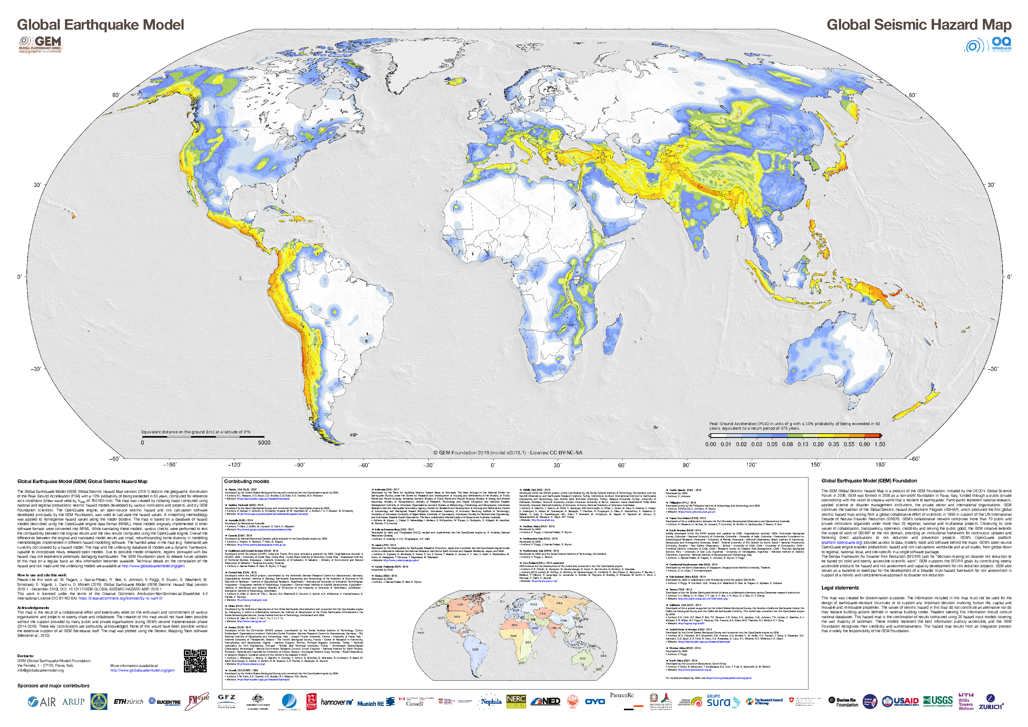
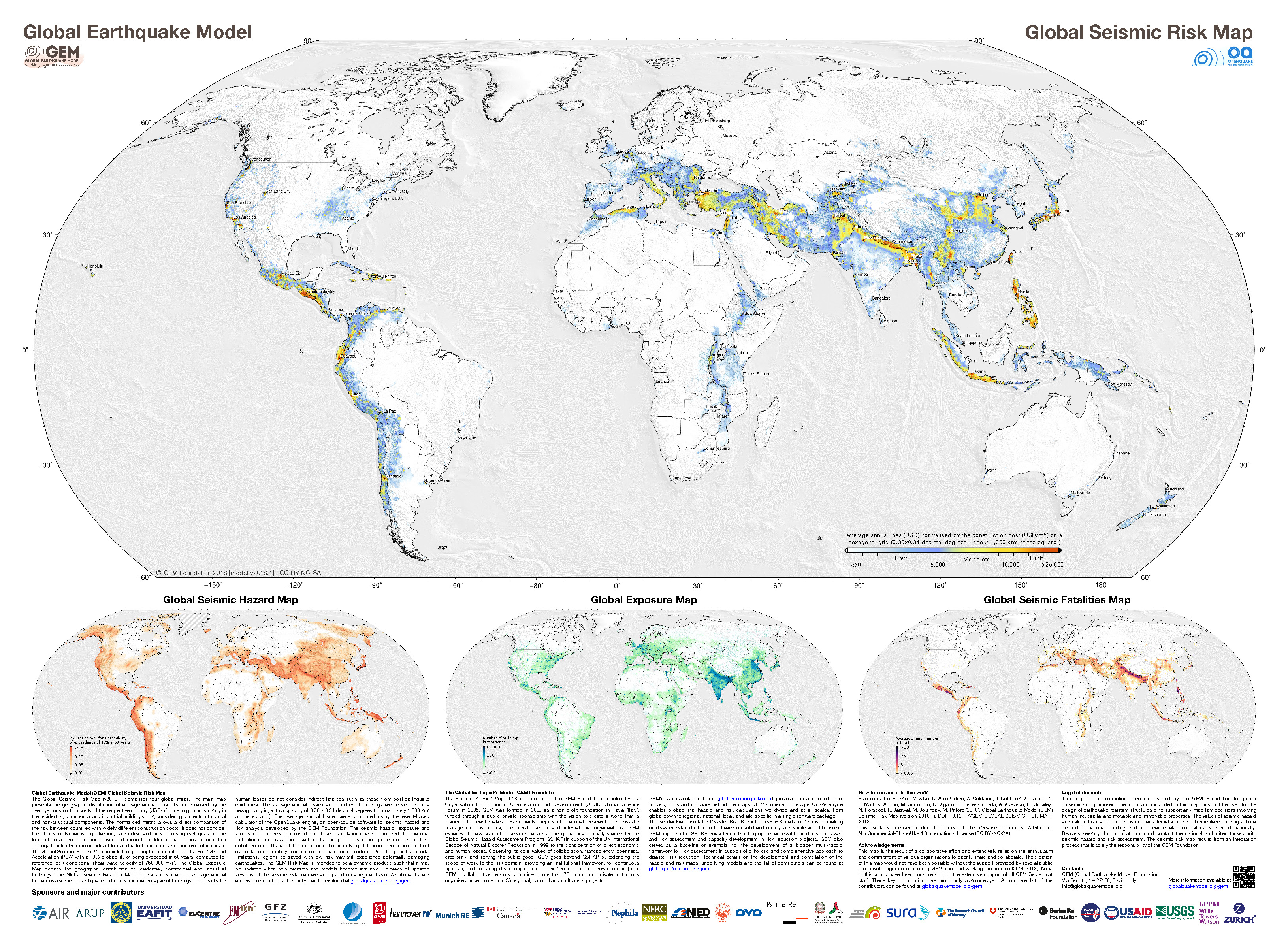
- These are the two maps shown in the map above, the GEM Seismic Hazard and the GEM Seismic Risk maps from Pagani et al. (2018) and Silva et al. (2018).
- The GEM Seismic Hazard Map:
- The Global Earthquake Model (GEM) Global Seismic Hazard Map (version 2018.1) depicts the geographic distribution of the Peak Ground Acceleration (PGA) with a 10% probability of being exceeded in 50 years, computed for reference rock conditions (shear wave velocity, VS30, of 760-800 m/s). The map was created by collating maps computed using national and regional probabilistic seismic hazard models developed by various institutions and projects, and by GEM Foundation scientists. The OpenQuake engine, an open-source seismic hazard and risk calculation software developed principally by the GEM Foundation, was used to calculate the hazard values. A smoothing methodology was applied to homogenise hazard values along the model borders. The map is based on a database of hazard models described using the OpenQuake engine data format (NRML). Due to possible model limitations, regions portrayed with low hazard may still experience potentially damaging earthquakes.
- Here is a view of the GEM seismic hazard map for Indonesia and the Philippines.
- The GEM Seismic Risk Map:
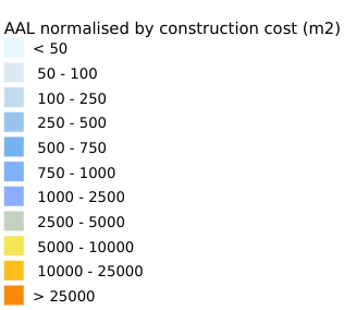
- The Global Seismic Risk Map (v2018.1) presents the geographic distribution of average annual loss (USD) normalised by the average construction costs of the respective country (USD/m2) due to ground shaking in the residential, commercial and industrial building stock, considering contents, structural and non-structural components. The normalised metric allows a direct comparison of the risk between countries with widely different construction costs. It does not consider the effects of tsunamis, liquefaction, landslides, and fires following earthquakes. The loss estimates are from direct physical damage to buildings due to shaking, and thus damage to infrastructure or indirect losses due to business interruption are not included. The average annual losses are presented on a hexagonal grid, with a spacing of 0.30 x 0.34 decimal degrees (approximately 1,000 km2 at the equator). The average annual losses were computed using the event-based calculator of the OpenQuake engine, an open-source software for seismic hazard and risk analysis developed by the GEM Foundation. The seismic hazard, exposure and vulnerability models employed in these calculations were provided by national institutions, or developed within the scope of regional programs or bilateral collaborations.
- Here is a view of the GEM seismic risk map for Indonesia and the Philippines.


Potential for Ground Failure
- Below are a series of maps that show the potential for landslides and liquefaction. These are all USGS data products.
There are many different ways in which a landslide can be triggered. The first order relations behind slope failure (landslides) is that the “resisting” forces that are preventing slope failure (e.g. the strength of the bedrock or soil) are overcome by the “driving” forces that are pushing this land downwards (e.g. gravity). The ratio of resisting forces to driving forces is called the Factor of Safety (FOS). We can write this ratio like this:FOS = Resisting Force / Driving Force
- When FOS > 1, the slope is stable and when FOS < 1, the slope fails and we get a landslide. The illustration below shows these relations. Note how the slope angle α can take part in this ratio (the steeper the slope, the greater impact of the mass of the slope can contribute to driving forces). The real world is more complicated than the simplified illustration below.
- Landslide ground shaking can change the Factor of Safety in several ways that might increase the driving force or decrease the resisting force. Keefer (1984) studied a global data set of earthquake triggered landslides and found that larger earthquakes trigger larger and more numerous landslides across a larger area than do smaller earthquakes. Earthquakes can cause landslides because the seismic waves can cause the driving force to increase (the earthquake motions can “push” the land downwards), leading to a landslide. In addition, ground shaking can change the strength of these earth materials (a form of resisting force) with a process called liquefaction.
- Sediment or soil strength is based upon the ability for sediment particles to push against each other without moving. This is a combination of friction and the forces exerted between these particles. This is loosely what we call the “angle of internal friction.” Liquefaction is a process by which pore pressure increases cause water to push out against the sediment particles so that they are no longer touching.
- An analogy that some may be familiar with relates to a visit to the beach. When one is walking on the wet sand near the shoreline, the sand may hold the weight of our body generally pretty well. However, if we stop and vibrate our feet back and forth, this causes pore pressure to increase and we sink into the sand as the sand liquefies. Or, at least our feet sink into the sand.
- Below is a diagram showing how an increase in pore pressure can push against the sediment particles so that they are not touching any more. This allows the particles to move around and this is why our feet sink in the sand in the analogy above. This is also what changes the strength of earth materials such that a landslide can be triggered.
- Below is a diagram based upon a publication designed to educate the public about landslides and the processes that trigger them (USGS, 2004). Additional background information about landslide types can be found in Highland et al. (2008). There was a variety of landslide types that can be observed surrounding the earthquake region. So, this illustration can help people when they observing the landscape response to the earthquake whether they are using aerial imagery, photos in newspaper or website articles, or videos on social media. Will you be able to locate a landslide scarp or the toe of a landslide? This figure shows a rotational landslide, one where the land rotates along a curvilinear failure surface.
- Below is the liquefaction susceptibility and landslide probability map (Jessee et al., 2017; Zhu et al., 2017). Please head over to that report for more information about the USGS Ground Failure products (landslides and liquefaction). Basically, earthquakes shake the ground and this ground shaking can cause landslides.
- I use the same color scheme that the USGS uses on their website. Note how the areas that are more likely to have experienced earthquake induced liquefaction are in the valleys. Learn more about how the USGS prepares these model results here.


- 2023.12.02 M 7.6 Philippines
- 2022.07.27 M 7.0 Philippines (poster)
- 2021.08.11 M 7.1 Philippines (poster)
- 2019.11.14 M 7.1 Halmahera
- 2019.07.14 M 7.3 Halmahera
- 2018.12.29 M 7.0 Philippines
- 2017.12.08 M 6.5 Caroline Ridge
- 2017.12.09 M 6.5 Caroline Ridge Update #1
- 2017.08.11 M 6.2 Philippines
- 2017.04.28 M 6.9 Philippines
- 2017.04.08 M 5.9 Philippines
- 2017.01.10 M 7.3 Celebes Sea
- 2016.07.29 M 7.7 Mariana
- 2015.03.17 M 6.2 Molucca Sea
- 2014.11.26 M 6.8 Molucca Sea
- 2014.11.21 M 6.5 Molucca Sea
- 2014.11.15 M 7.1 Molucca Sea
Philippines | Western Pacific
Earthquake Reports
Social Media
#EarthquakeReport for M7.6 #Lindol #Earthquake offshore of #Philippines
Widely felt
Reported intensity MMI 7 so far
Probably will generate tsunami2018 report has tectonic background information https://t.co/wr5A0HdqI1https://t.co/tAksqwTFvd pic.twitter.com/P3CZomI9F6
— Jason "Jay" R. Patton (@patton_cascadia) December 2, 2023
#EarthquakeReport for M7.6 #Lindol #Earthquake offshore of #Philippines
Pacific Tsunami Warning Center notification
Probably will generate tsunami in regions listed2018 report has tectonic background information https://t.co/wr5A0HdqI1https://t.co/gMQt8te0ae pic.twitter.com/k4gCqXCMNz
— Jason "Jay" R. Patton (@patton_cascadia) December 2, 2023
#EarthquakeReport for M7.6 #Lindol #Earthquake offshore of the #Philippines
generated ~10cm amplitude (20cm wave height) tsunami at Davao Tide Gage (which is in a somewhat sheltered location compared to epicenter so probably larger tsunami along coast)https://t.co/gVDP4iJO55 pic.twitter.com/Dm4DdbxpYe
— Jason "Jay" R. Patton (@patton_cascadia) December 2, 2023
#EarthquakeReport #TsunamiReport for M 7.4 #Lindol #Earthquake offshore of #Mindanao #Philippines
compressional (thrust) earthquake
generated tsunami@USGS_Quakes models suggest high chance for liquefaction
triggered slip near interface (?)report here:https://t.co/CVr22I6vTa pic.twitter.com/WLJw0BLJKv
— Jason "Jay" R. Patton (@patton_cascadia) December 3, 2023
Information Statement Tsunami Info Stmt: M7.7 Mindanao, Philippine Islands 0637PST Dec 2: Tsunami NOT expected
— NWS Tsunami Alerts (@NWS_NTWC) December 2, 2023
M 7.6 – Mindanao, Philippineshttps://t.co/7lON8jKAk6 pic.twitter.com/ZUvRWAitWE
— Wendy Bohon, PhD 🌏 (@DrWendyRocks) December 2, 2023
Mw=7.6, MINDANAO, PHILIPPINES (Depth: 32 km), 2023/12/02 14:37:03 UTC – Full details here: https://t.co/pzEI19fPy5 pic.twitter.com/r4Qgy4i3rP
— Earthquakes (@geoscope_ipgp) December 2, 2023
Waves from the M7.6 earthquake in the Philippines shown on a nearby seismic station using Station Monitor
➡️ https://t.co/Tir0KZELXN pic.twitter.com/HFKRH3miN0
— EarthScope Consortium (@EarthScope_sci) December 2, 2023
The Pacific Tsunami Warning Center is monitoring the potential for a Tsunami threat for the Republic of Palau as well as the CNMI , Yap State, and Guam due to a 7.7 magnitude earthquake at 12:37 am ChST at Minadao, Philippines. For more information, please visit our website. pic.twitter.com/7fzoT2ppNg
— NWS Guam 🇬🇺 (@NWSGuam) December 2, 2023
Auto solution FMNEAR (Géoazur/OCA) with regional records for the M 7.5 – MINDANAO, PHILIPPINES – 2023-12-02 14:37:08.0 UTC (Loc EMSC used to trigger inversion).
Thanks to the seismic records by GFZ and IRIS
Note the absence of available regional stations in the North pic.twitter.com/SBoYefpiBe
— Bertrand Delouis (@BertrandDelouis) December 2, 2023
Major M7.5+, intermediate depth, vertical-up (reverse) faulting #earthquake at 10cm/y Philippine plate convergence zone. Just offshore populated region with moderate land surface shaking and significant tsunami potential. https://t.co/aqR4m0n22B#philippines #geohazards pic.twitter.com/JWSfNiX5eb
— 🌎 Prof Ben van der Pluijm ⚒️ (@vdpluijm) December 2, 2023
A 7.7 magnitude earthquake occurred at 4:37 AM HST 12/02 in Mindanao, Philippines. There is NO tsunami threat to Hawaiʻi. pic.twitter.com/I1zjgstJoJ
— Hawaii EMA (@Hawaii_EMA) December 2, 2023
One hour and half ago, Mw7.5 #earthquake near eastern coast of Mindanao, Philippines. Although not shallow, could be very damaging, due to magnitude and location. Felt as far as southern Luzon. #Tsunami expected. Similar EQ in 1989.https://t.co/suPwwcXQZHhttps://t.co/TQm681XoBK pic.twitter.com/KF4uT50YuC
— José R. Ribeiro (@JoseRodRibeiro) December 2, 2023
M 7.4 – Mindanao, Philippines pic.twitter.com/m0Htkzmx87
— DARYONO BMKG (@DaryonoBMKG) December 2, 2023
ADVISORY: TSUNAMI WARNING
Tsunami Information No.1
Date and Time: 02 Dec 2023 – 10:37 PM
Magnitude = 6.9
Depth = 008 kilometers
Location = 08.52°N, 126.69°E – Offshore of Surigao Del Surhttps://t.co/YnEUN7M8Qs pic.twitter.com/C3Ris1BCVp— PHIVOLCS-DOST (@phivolcs_dost) December 2, 2023
Preliminary M7.7 #Earthquake
ID: #rs2023xsbiqf
Mindanao, Philippines
2023-12-02 14:37 UTC@raspishake #QuakeView– Learn more about us at https://t.co/ojzht2DDAL
– EVENT: https://t.co/EGCrzKNHQX pic.twitter.com/924Oxw1TSw
— Raspberry Shake Earthquake Channel (@raspishakEQ) December 2, 2023
In this video you can watch the waves from the M7.6 earthquake off the coast of Mindanao, Philippines sweep across seismic stations in North America and Europe. Animations from @EarthScope_sci can be found at https://t.co/h74rgO7ZKf pic.twitter.com/DqU0crRjhM
— Wendy Bohon, PhD 🌏 (@DrWendyRocks) December 2, 2023
On 02 Dec 2023, 10:37 PM (local time), a Mw 7.4 earthquake with a depth of 25-30 km hit Eastern Mindanao, Philippines. As of 03 Dec 2023, 4:30 am, there were already two M>6 and several M>5 aftershocks. The earthquake is associated with the subduction along the Philippine Trench. pic.twitter.com/0iyMH5cMHs
— Deo (@deotectonics) December 2, 2023
Since the M7.5 Philippines earthquake ~7 hrs ago, there have been ~30 aftershocks greater than M5.0, most of which can easily be seen in the data from the @AusQuake seismometers in southeast Australia. pic.twitter.com/z72xk0Bc7M
— Dr. Dee Ninis (@DeeNinis) December 2, 2023
Watch the waves from the M7.6 earthquake in the Philippines roll across seismic stations in North America. (THREAD 🧵) pic.twitter.com/NJNRY0UhkQ
— EarthScope Consortium (@EarthScope_sci) December 2, 2023
Recent Earthquake Teachable Moment for the M7.6 earthquake in the Philippines.
Teachable Moments presentations capture the opportunity to bring knowledge, insight, and critical thinking to the classroom following a newsworthy earthquake.
➡️ https://t.co/a4C3tydbsc pic.twitter.com/jyyjpVLvH4
— EarthScope Consortium (@EarthScope_sci) December 2, 2023
Over the last 7 hours there have been dozens of earthquakes off the southeast coast of the Philippines. Traces are from a station in South Australia. The largest was a magnitude 7.4 on hour 14. The quake on hour 12 is a magnitude 5.8 earthquake in the Banda Sea, north of Darwin pic.twitter.com/yk2VEmXTTO
— Adam Pascale (@SeisLOLogist) December 2, 2023
Mindanao Shake Map – potential to damage pic.twitter.com/YnXyJsAkuD
— DARYONO BMKG (@DaryonoBMKG) December 2, 2023
2023-12-02 M7.6 Mindanao, #Philippines #earthquake recorded in #Scotland & #Stornoway + historical seismicity & cross section.
On the edge of the shadow zone from here.
Dist.: 11450.9km
Travel Time: 14m 0.4s
Depth: 32.763km#Python @raspishake @matplotlib #CitizenScience pic.twitter.com/btGMvb6FSy— Giuseppe Petricca (@gmrpetricca) December 2, 2023
UPDATE: 4 Dec 2023
Yesterday's M7.6 earthquake in the Philippines raised high alerts, but damage has been lower than expected. Why? We think the USGS overestimated shaking due to lack of seismometers. The slab model here also seems too deep, perhaps by ~20 km. Read more on our blog; link in my bio. pic.twitter.com/qQBcPhgxBV
— Dr. Judith Hubbard (@JudithGeology) December 3, 2023
The seismic activity after the 2023-12-02 M7.6 Mindanao, #Philippines #earthquake. Almost 300 detected shocks in the past 54 hours.
The infographic shows the events' area distribution with daily & magnitude data.#Python @matplotlib #CitizenScience pic.twitter.com/c4iCULVB1M
— Giuseppe Petricca (@gmrpetricca) December 4, 2023
- Frisch, W., Meschede, M., Blakey, R., 2011. Plate Tectonics, Springer-Verlag, London, 213 pp.
- Hayes, G., 2018, Slab2 – A Comprehensive Subduction Zone Geometry Model: U.S. Geological Survey data release, https://doi.org/10.5066/F7PV6JNV.
- Holt, W. E., C. Kreemer, A. J. Haines, L. Estey, C. Meertens, G. Blewitt, and D. Lavallee (2005), Project helps constrain continental dynamics and seismic hazards, Eos Trans. AGU, 86(41), 383–387, , https://doi.org/10.1029/2005EO410002. /li>
- Jessee, M.A.N., Hamburger, M. W., Allstadt, K., Wald, D. J., Robeson, S. M., Tanyas, H., et al. (2018). A global empirical model for near-real-time assessment of seismically induced landslides. Journal of Geophysical Research: Earth Surface, 123, 1835–1859. https://doi.org/10.1029/2017JF004494
- Kreemer, C., J. Haines, W. Holt, G. Blewitt, and D. Lavallee (2000), On the determination of a global strain rate model, Geophys. J. Int., 52(10), 765–770.
- Kreemer, C., W. E. Holt, and A. J. Haines (2003), An integrated global model of present-day plate motions and plate boundary deformation, Geophys. J. Int., 154(1), 8–34, , https://doi.org/10.1046/j.1365-246X.2003.01917.x.
- Kreemer, C., G. Blewitt, E.C. Klein, 2014. A geodetic plate motion and Global Strain Rate Model in Geochemistry, Geophysics, Geosystems, v. 15, p. 3849-3889, https://doi.org/10.1002/2014GC005407.
- Meyer, B., Saltus, R., Chulliat, a., 2017. EMAG2: Earth Magnetic Anomaly Grid (2-arc-minute resolution) Version 3. National Centers for Environmental Information, NOAA. Model. https://doi.org/10.7289/V5H70CVX
- Müller, R.D., Sdrolias, M., Gaina, C. and Roest, W.R., 2008, Age spreading rates and spreading asymmetry of the world’s ocean crust in Geochemistry, Geophysics, Geosystems, 9, Q04006, https://doi.org/10.1029/2007GC001743
- Pagani,M. , J. Garcia-Pelaez, R. Gee, K. Johnson, V. Poggi, R. Styron, G. Weatherill, M. Simionato, D. Viganò, L. Danciu, D. Monelli (2018). Global Earthquake Model (GEM) Seismic Hazard Map (version 2018.1 – December 2018), DOI: 10.13117/GEM-GLOBAL-SEISMIC-HAZARD-MAP-2018.1
- Silva, V ., D Amo-Oduro, A Calderon, J Dabbeek, V Despotaki, L Martins, A Rao, M Simionato, D Viganò, C Yepes, A Acevedo, N Horspool, H Crowley, K Jaiswal, M Journeay, M Pittore, 2018. Global Earthquake Model (GEM) Seismic Risk Map (version 2018.1). https://doi.org/10.13117/GEM-GLOBAL-SEISMIC-RISK-MAP-2018.1
- Zhu, J., Baise, L. G., Thompson, E. M., 2017, An Updated Geospatial Liquefaction Model for Global Application, Bulletin of the Seismological Society of America, 107, p 1365-1385, https://doi.org/0.1785/0120160198
- Bock et al., 2003. Crustal motion in Indonesia from Global Positioning System measurements in JGR, v./ 108, no. B8, 2367, doi:10.1029/2001JB000324
- Hall, R., 2011. Australia–SE Asia collision: plate tectonics and crustal flow in Hall, R., Cottam, M. A. &Wilson, M. E. J. (eds) The SE Asian Gateway: History and Tectonics of the Australia–Asia Collision. Geological Society, London, Special Publications, 355, 75–109.
- Fan, J-k., Wu, S-g., Spence, G., 2015. Tomographic evidence for a slab tear induced by fossil ridge subduction at Manila Trench, South China Sea in International Geology Review, v. 57, p. 998-1013, DOI: 10.1080/00206814.2014.929054
- Hayes, G.P., Wald, D.J., and Johnson, R.L., 2012. Slab1.0: A three-dimensional model of global subduction zone geometries in, J. Geophys. Res., 117, B01302, doi:10.1029/2011JB008524
- Hsu, Y-J., Yu, S-B., Song, T-R.A., and Bacolcol, T., 2012. Plate coupling along the Manila subduction zone between Taiwan and northern Luzo in Journal of Asian Earth Sciences, v. 51, p. 98-108
- McCaffrey, R., Silver, E.A., and Raitt, R.W., 1980. Crustal Structure of the Molucca Sea Collision Zone, Indonesia in The Tectonic and Geologic Evolution of Southeast Asian Seas and Islands-Geophysical Monograph 23, p. 161-177.
- Noda, A., 2013. Strike-Slip Basin – Its Configuration and Sedimentary Facies in Mechanism of Sedimentary Basin Formation – Multidisciplinary Approach on Active Plate Margins http://www.intechopen.com/books/mechanism-of-sedimentarybasin-formation-multidisciplinary-approach-on-active-plate-margins http://dx.doi.org/10.5772/56593
- Smoczyk, G.M., Hayes, G.P., Hamburger, M.W., Benz, H.M., Villaseñor, Antonio, and Furlong, K.P., 2013. Seismicity of the Earth 1900–2012 Philippine Sea plate and vicinity: U.S. Geological Survey Open-File Report 2010–1083-M, 1 sheet, scale 1:10,000,000.
- Waltham et al., 2008. Basin formation by volcanic arc loading in GSA Special Papers 2008, v. 436, p. 11-26.
- Wang, K., and Bilek, S.L., 2014. Invited review paper: Fault creep caused by subduction of rough seafloor relief in Tectonophysics, v. 610, p./ 1-24.
- Wu, J., J. Suppe, R. Lu, and R. Kanda, 2016. Philippine Sea and East Asian plate tectonics since 52 Ma constrained by new subducted slab reconstruction methods, J. Geophys. Res. Solid Earth, 121, doi:10.1002/2016JB012923.
- Zahirovic et al., 2014. The Cretaceous and Cenozoic tectonic evolution of Southeast Asia in Solid Earth, v. 5, p. 227-273, doi:10.5194/se-5-227-2014.
References:
Basic & General References
Specific References
Return to the Earthquake Reports page.
- Sorted by Magnitude
- Sorted by Year
- Sorted by Day of the Year
- Sorted By Region