I present this summary of the Earthquake Reports and Interpretive Posters I prepared for earthquakes during the year 2019.
First is the Earthquake Report Map Interface. Earthquake epicenters for each Earthquake Report and Interpretive Poster are plotted on a map.
The embedded map is very small, which makes it difficult to use. Click on the “larger map“ link to see this online map interface in a larger format within it’s own window.
One may click on the epicenter dots to learn more about that earthquake. Some Basic Information Shows up in a query window:
- Date and Time
- Name and Magnitude
- Depth
- Link to Earthquake Report Page
- Link to Interpretive Poster (pdf)
- Link to USGS Earthquake Page
Below the map interface is a summary of the Earthquake Reports and Interpretive Posters. There are links to the reports, summaries of the earthquakes, and links to the main posters for these events.
- Here are all the annual summaries:
- Here are the annual summaries for the Cascadia region.
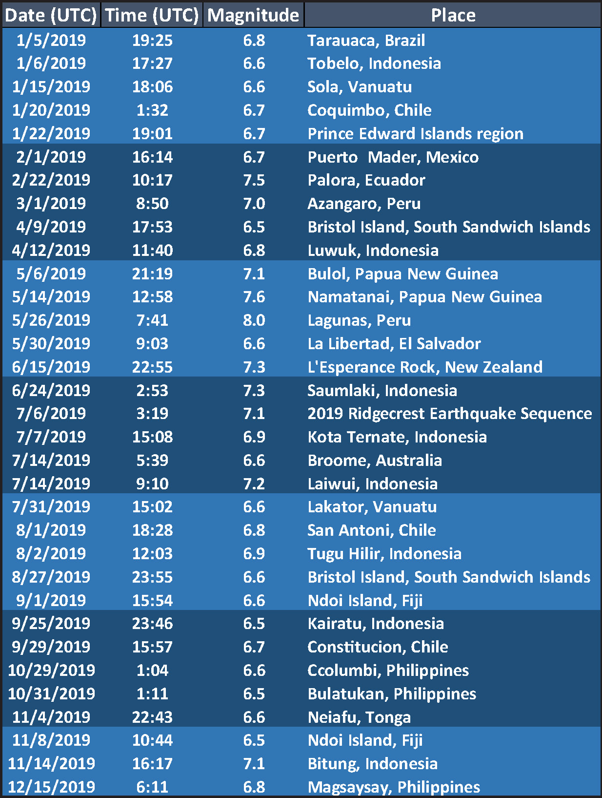
- Here is a table that lists the 2019 earthquakes with magnitudes M ≥ 6.5. I use these earthquakes to plot the cumulative energy release for earthquakes below.
- This is a plot showing the cumulative energy release (in Joules) for the earthquakes listed in the above table. Ask yourself if M 6.5 is a reasonable threshold to be able to visualize variations in seismic energy release during the year.

2019 Earthquake Reports
- 2019.11.26 M 6.4 Albania
- 2019.11.14 M 7.1 Halmahera
- 2019.09.24 M 6.0 Puerto Rico (Mona Passage) Poster
- 2019.08.29 M 6.3 Blanco transform fault
- 2019.08.02 M 6.9 Indonesia
- 2019.08.01 M 6.8 Chile
- 2019.07.14 M 7.3 Halmahera
- 2019.07.04 M 6.4 Ridgecrest
- 2019.07.05 M 6.4 / 7.1 Ridgecrest Update #1
- 2019.07.18 M 6.4 / 7.1 Ridgecrest Update #2
- 2019.07.20 M 6.4 / 7.1 Ridgecrest Update #3
- 2019.06.23 M 7.3 Banda Sea
- 2019.06.23 M 5.6 Petrolia
- 2019.06.15 M 7.2 Kermadec
- 2019.06.14 M 6.4 Chile
- 2019.06.05 M 4.3 San Clemente Island
- 2019.05.26 M 8.0 Peru
- 2019.05.14 M 7.5 New Ireland
- 2019.05.12 M 6.1 Panama
- 2019.05.06 M 7.2 Papua New Guinea
- 2019.04.12 M 6.8 Sulawesi, Indonesia
- 2019.04.02 M 6.5 Aleutians
- 2019.03.26 M 5.2 Alaska
- 2019.03.01 M 7.0 Peru
- 2019.02.22 M 7.5 Ecuador
- 2019.02.01 M 6.6 Guatemala & Mexico
- 2019.01.20 M 6.7 Chile
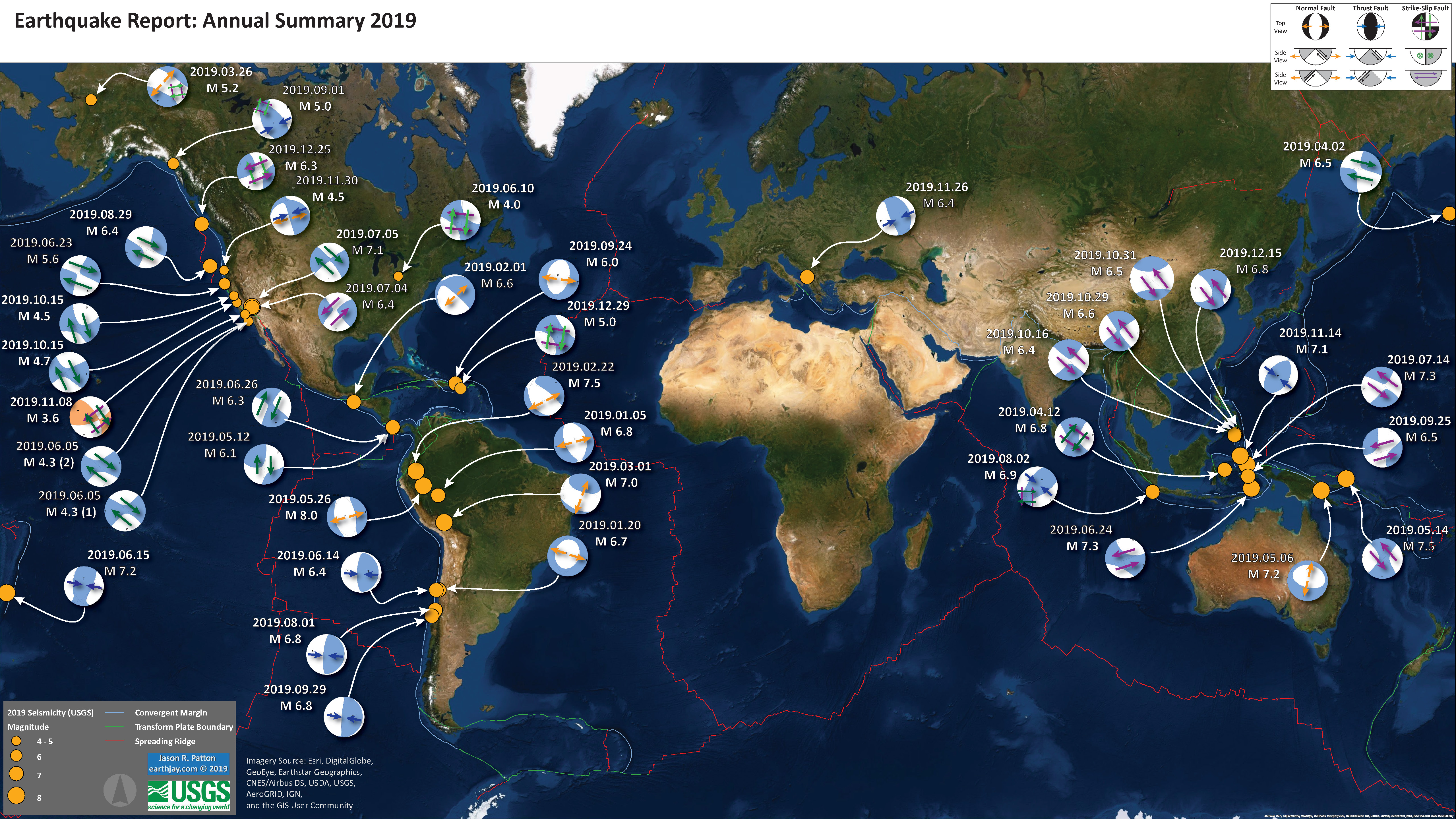
Annual Summary Poster
2019 Earthquake Report Map Interface
The orange circles are epicenters from the selected earthquakes. Click on the epicenter to learn more about that earthquake event. I need to update this with some earthquakes in December.
- Click here to open a larger version of this web map.
Other Annual Summaries
Earthquakes in/near southwest #BritishColumbia during 2019. An average year…
589 earthquakes (the largest was M6.2), only 7 were felt. This is a region of active plate tectonics.
M6-6.9: 2
M5-5.9: 8
M4-4.9: 15
M3-3.9: 111
Some details: https://t.co/CwgiLHdNQA#NRCanSci pic.twitter.com/XB158CrvDf— John Cassidy (@earthquakeguy) December 31, 2019
A look back at the year’s earthquakes as the minutes left in 2019 tick down. Typical numbers for the year: 1 M8, 9 M7s, 133 M6s, etc. But mercifully few fatalities due to remote locations or deeper depths of the largest quakes. A lucky year. pic.twitter.com/NsCpIeQN6H
— Susan Hough (@SeismoSue) December 31, 2019
Damaging earthquakes 2019: 299 quakes (M1.7-8.0), 289 casualties, 274.000 damaged buildings, 59 affected countries. More details in the next days… #EarthquakeImpactDatabase@CATnewsDE @LastQuake @ISCseism @IRIS_EPO @GFZ_Potsdam @UKEQ_Bulletin
Database: https://t.co/nXLgGAxA0U pic.twitter.com/mZXVHUnA4x— Erdbebennews (@Erdbebennews) January 1, 2020
184 regional moment tensor solutions for New Zealand earthquakes in 2019. Mw 2.9 – 7.3 and depths 2 – 280 km. The largest events were to in the north in the Kermadec trench; however, there were several M 5+ events onshore or close to land. pic.twitter.com/OmeEPly0CE
— John Ristau 🇨🇦 🇳🇿 (@SinistralSeismo) January 6, 2020
With more than 50,000 earthquakes, 2019 finished as the second highest year on record!
Seismicity was dominated by aftershock sequences continuing from 2018 earthquakes and two notable swarms. The Purcell Mountain swarm alone accounted for more than 10% of the total. pic.twitter.com/98r3xCKrFY— Alaska Earthquake Center (@AKearthquake) January 24, 2020
Earthquake Reports
Interpretive Poster Background
These Interpretive Posters all contain slightly different types and amounts of information. Below is a general guidance to what this information is. Earthquake Report pages can provide additional information about each individual interpretive interrogation.
- I plot the seismicity from the past month, with color representing depth and diameter representing magnitude (see legend). I may include historic earthquake epicenters with magnitudes M ≥ some magnitude threshold.
- I include background information from published papers as inset figures on the interpretive posters. Learn more about these figures in their associated Earthquake Report.
- I plot the USGS fault plane solutions (moment tensors in blue and focal mechanisms in orange), possibly in addition to some relevant historic earthquakes.
- A review of the basic base map variations and data that I use for the interpretive posters can be found on the Earthquake Reports page.
- Some basic fundamentals of earthquake geology and plate tectonics can be found on the Earthquake Plate Tectonic Fundamentals page.
See all 2019 Earthquake Reports and Interpretive Posters sorted by time:
If there is an existing Earthquake Report Page, the magnitude and earthquake location will be a link in light green. Click on that link to go to the Earthquake Report Page.
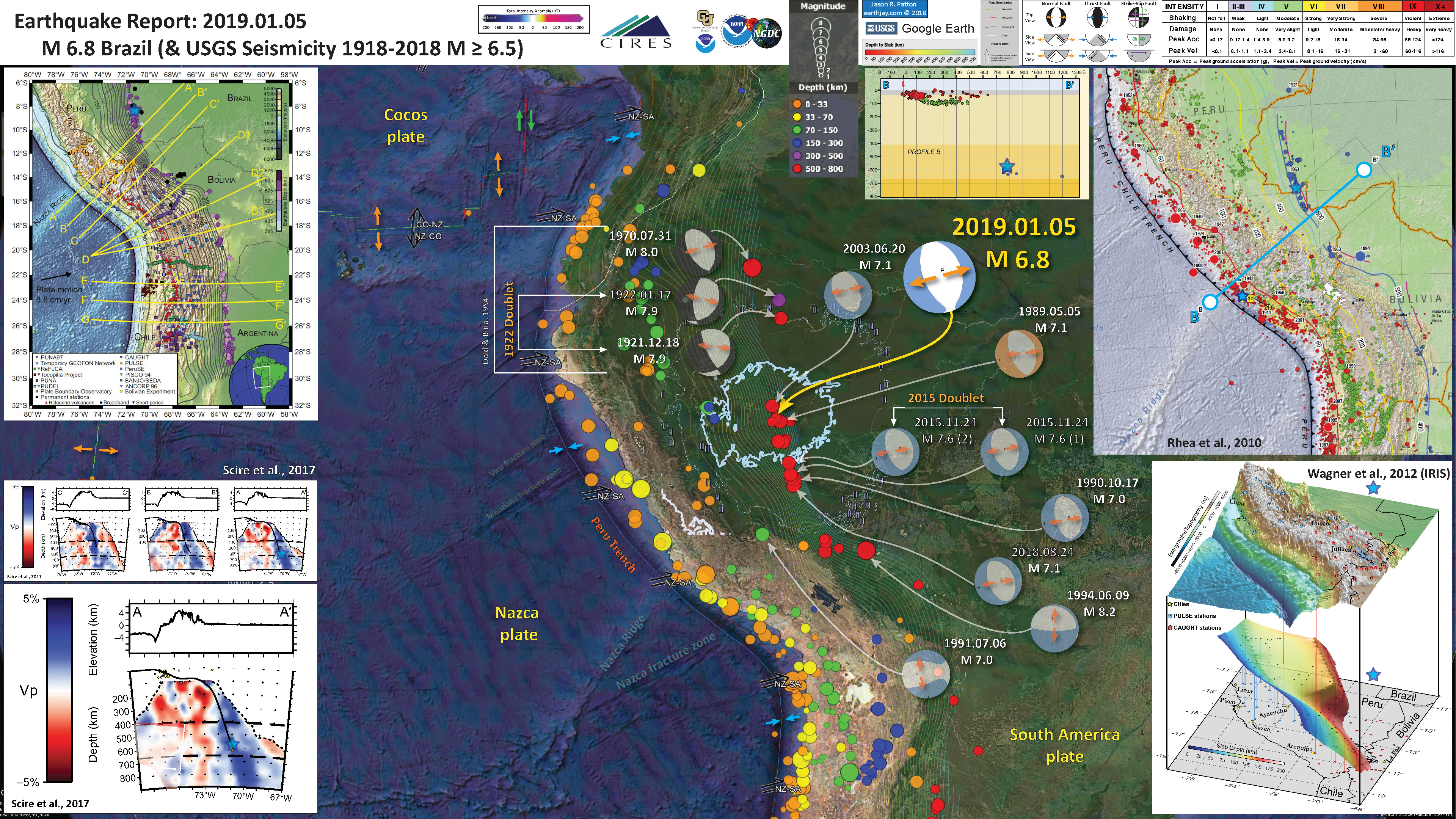
- 2019.01.05 M 6.8 Brazil
https://earthquake.usgs.gov/earthquakes/eventpage/us2000j0ja/executive
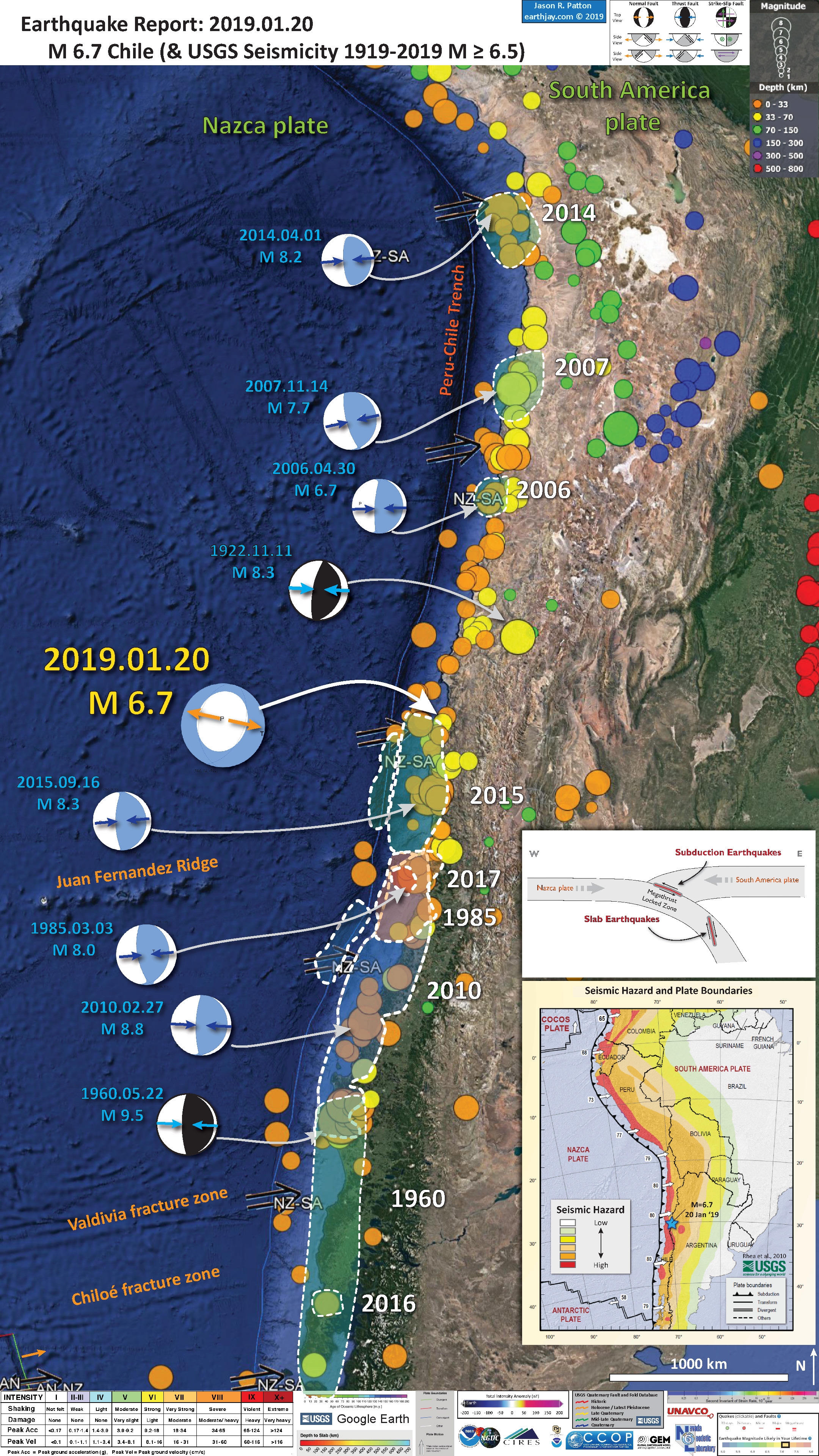
- 2019.01.20 M 6.7 Chile
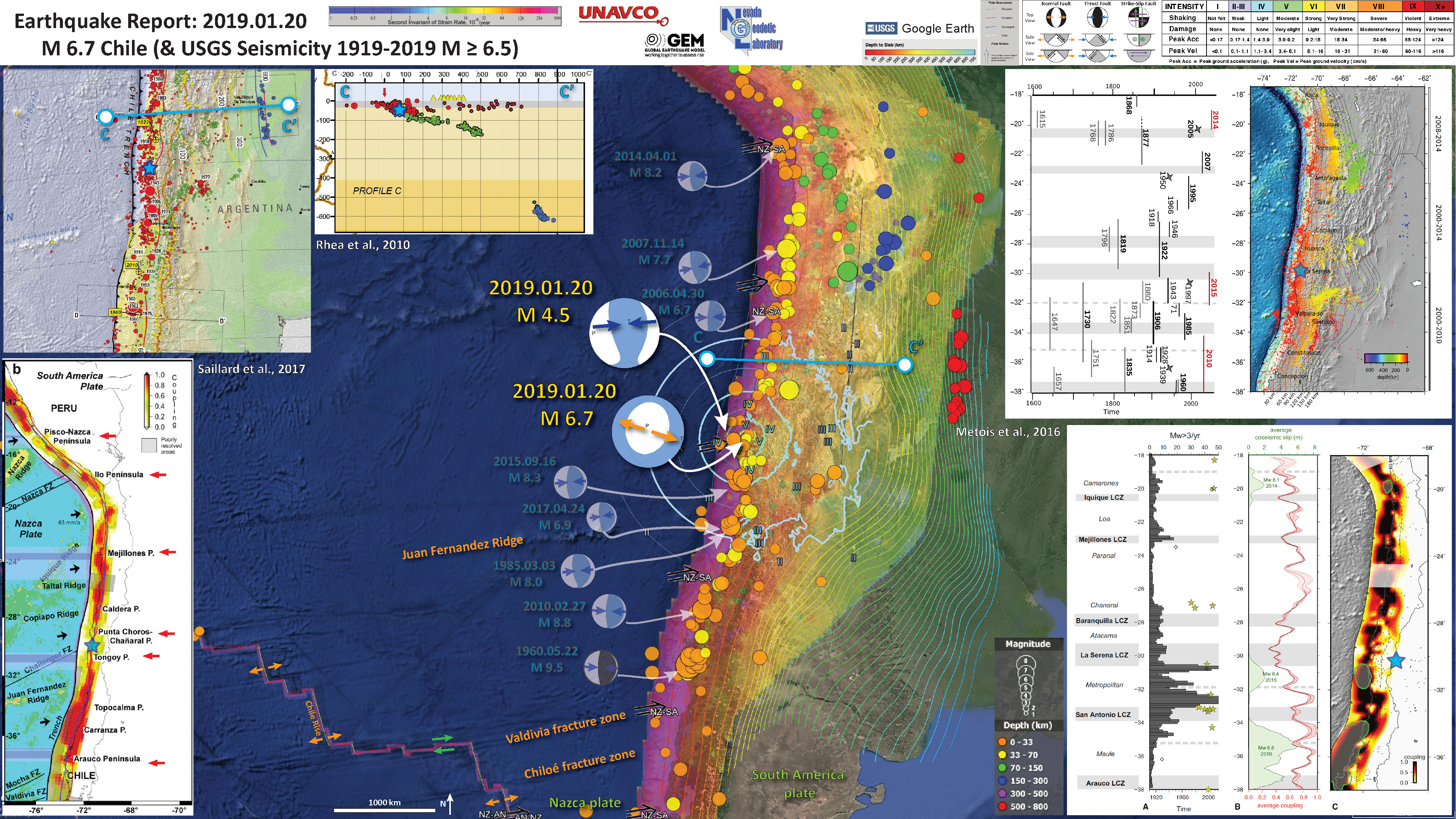
- The quake is extensional, while on a convergent plate boundary. This could possibly be due to slab pull (the downgoing plate pulls downwards, causing extension in the plate).
- The quake was deep, so this tells us it is not a megathrust subduction zone earthquake (because megathrust earthquakes, quakes caused by slip between the plates, only occurs at shallower depths).
- The quake is in an area of the subduction zone that has not had a subduction zone earthquake since 1922.
- The quake happened in a region of low seismogenic coupling.
- The quake was at the edge of the aftershock zone from the 2015 M=8.3 subduction zone earthquake.
- There was an earthquake sequence in 1997 that may be an analogy to today’s M=6.7 quake (in ’97, a subduction zone earthquake sequence was followed by an along-strike (not down-dip) extensional sequence. While today was an extensional earthquake along strike from a subduction zone earthquake. However, it has been ~4 years between these two events. Is this too long? The 2015 is much larger than the 1997 sequence, so perhaps the static coulomb stress changes are more long lasting?)
- Here is the map with a century’s seismicity plotted with USGS epicenters for earthquakes M≥6.5.
- Here is the map with a month’s seismicity plotted. Also included in this poster is the global strain map. The second map includes the century’s historic seismicity.
- The Global Strain Map is a map product that tells us how much Earth’s crust is deforming due to plate tectonics. Areas that have more active faults are in regions of higher strain. Remember, strain is defined as a change in shape (e.g. length or volume) over time. When things deform more over a time period are in higher strain regions.
-
This M=6.7 earthquake is interesting for several reasons.

- 2019.02.01 M 6.6 Guatemala & Mexico
- Here is the map with a century’s seismicity plotted.
- Here is an interpretive poster showing how the 2017 June and September sequences spatially relate.
This morning (my time) there was a moderately deep earthquake along the coast of southern Mexico and northern Guatemala. Here is my Temblor article about this M=6.6 earthquake and how it might relate to the 2017 M=8.2 quake.
Offshore of Guatemala and Mexico, the Middle America trench is formed by the subduction of the oceanic Cocos plate beneath the North America and Caribbean plates.
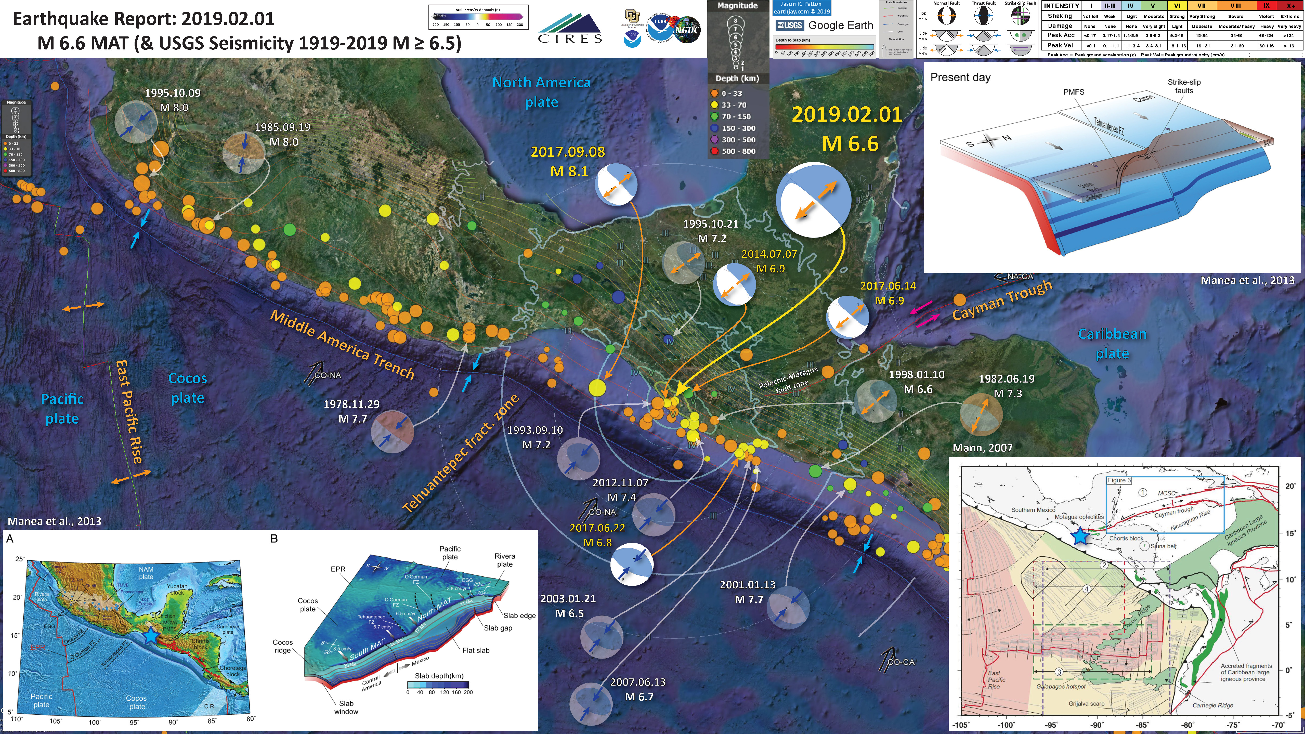
In 2017 there was a series of large magnitude earthquakes in the region of today’s M=6.6 and further to the south. These quakes are highlighted in the posters above, notable are the 6 Jun M=6.9 and 22 Jun M=6.8. The first quake was a deep extensional event, followed by a thrust event (possibly triggered by the M=6.9). In addition, there was a M=6.9 extensional earthquake in 2014 that also may have been a player.
I presented an interpretive poster showing the zone of aftershocks associated with the June sequence. Later, in Sept, there was a M=8.2 extensional tsunamigenic earthquake to the north of the June sequence. If we look at the aftershock zone for the M=8.2 quake, it looks like a sausage link adjacent to the sausage link formed by the June aftershocks. mmmm veggie sausages.
However there was no megathrust earthquake in the area of the M=8.2 sequence.
- 2019.02.22 M 7.5 Ecuador
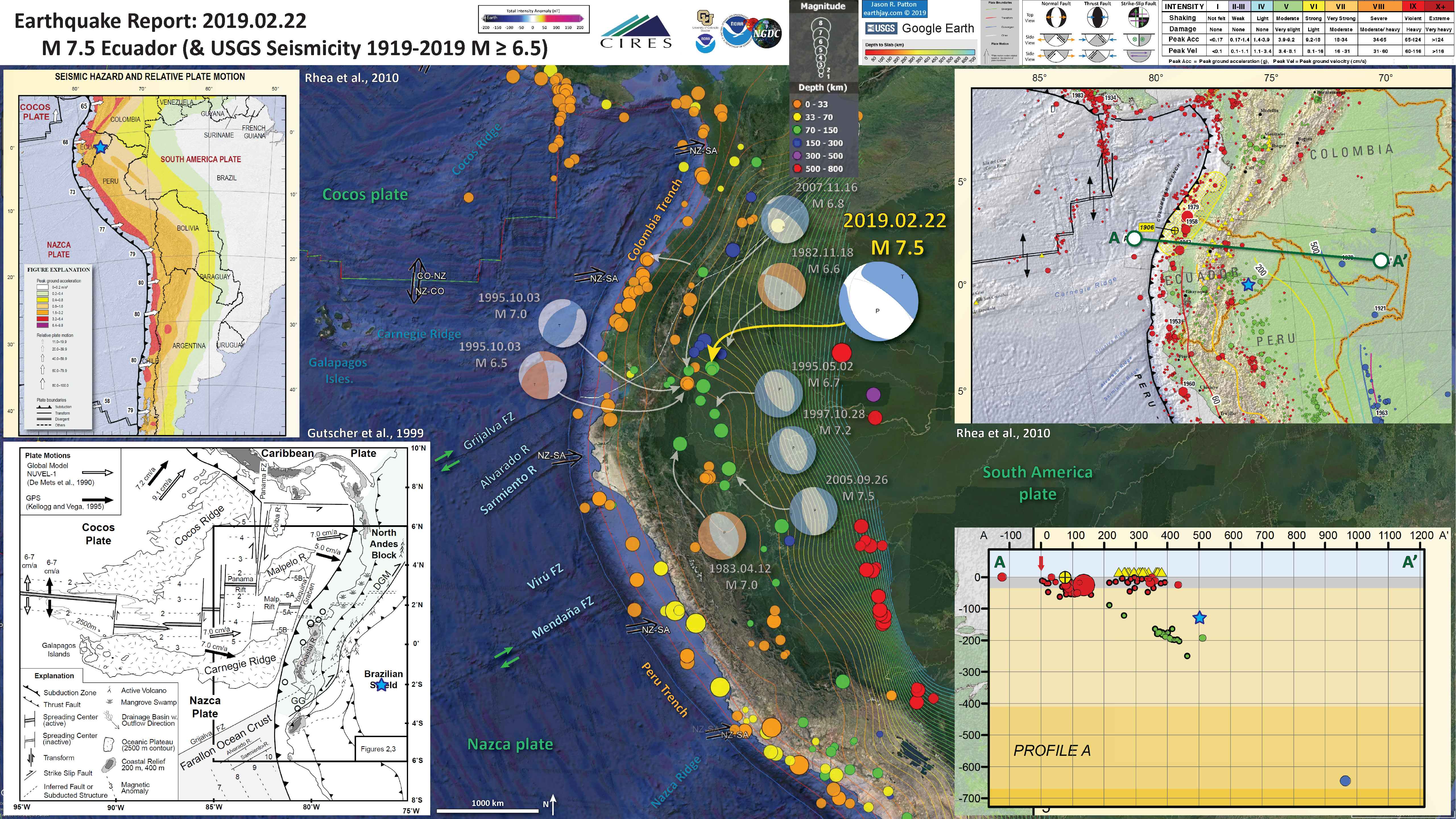
- In the historic earthquake poster below, check out how there are analogical earthquakes to today’s quake, while further to the south, these extensional quakes are oriented closer to being perpendicular to the trench.
- There are a few historic quakes on the map below that are thrust events (compressional), but they are much shallower in depth (about 17 and 24 km), compared to all other quakes are deeper than 70 km.
- Here is the map with a century’s seismicity plotted.
Well, as I was getting up this morning, my social media feed was abuzz about the intermediate depth earthquake in Peru. While it was quite deep (<130km), it was still widely felt and probably caused lots of damage.
This part of the world enjoys a variety of plate boundary fault systems and interesting plate tectonic interactions.
There are multiple spreading ridges, creating oceanic plates, and these ridges and plates interact in complicated ways. The results from these complicated relations (e.g. how a hotpot near a spreading ridge affects the thickness of the crust formed at that spreading ridge) can also impact the convergent plate boundaries as these plates subduct beneath the South America continental plate.
The subduction zone megathrust fault, formed where the Nazca plate dives under the South America plate, has an historic and prehistoric record of earthquakes. However, today's MW=7.5 earthquake is not a megathrust event.
The earthquake is an extensional (normal) type of an earthquake. It probably occurred along a fault in the downgoing Nazca plate.
The plate here is undergoing extension either from some internal deformation within the plate, or due to what we call “slab pull” (the plate that is diving down and deep is pulling the plate that is less deep). So, the fault may be oriented perpendicular to the direction the plate is going down. However, sometimes there are pre-existing faults (like fracture zones, etc.) that may reactivate under different conditions from when they were formed.
- 2019.03.01 M 7.0 Peru
- Here is the map with a century’s seismicity plotted.
On 01 March 2019 there was an intermediate depth earthquake near the border of Peru and Bolivia. In the past century, this is the first earthquake in this area at this depth. There are some historic quakes to the east, but they are much deeper. However, if we take a look at the 1994 M=8.2 shaker, it has a similar orientation as yesterday’s M=7.0 quake.
Another similarity with the 1994 temblor, is that they are both extensional (normal) earthquakes. The majority of intermediate depth earthquakes are extensional, but not all.

- 2019.03.26 M 5.2 Alaska
- Here is the map with a month’s seismicity plotted.
At shortly before 13:30 today in northern Alaska there was a large earthquake, with a magnitude of M=5.1.
Today’s earthquake happened away from one of the mapped faults in the USGS Quaternary Active Fault and Fold Database (the Kaltag fault). The earthquake mechanism shows this earthquake may have been a slightly oblique normal type of an earthquake. I placed strike-slip arrows on the 2 possible nodal planes.but this is mainly a normal earthquake.
There was also a normal earthquake in 1958, when a M=7.1 quake struck about 50 km (35 miles) to the southeast of today’s quake. However, the 1958 event was oriented perpendicular to today’s quake. Below are some observations made following the 1958 earthquake. There was evidence of liquefaction, with sand volcanoes about a meter thick extending for hundreds of meters laterally.

- 2019.04.02 M 6.5 Aleutians
- Here is the map with a month’s seismicity plotted. I outlined the blocks and labeled using Ryan and Scholl (1989) as a basemap (but very similar to Krutikov). I outlined some lineaments in the magnetic anomaly data for crust on both sides of the Amlia fracture zone and labeled these B and A (near label for Pacific plate). Note how they are offset relative to each other, demonstration of the left-lateral sense of motion here.
- Here is the map with a century’s seismicity plotted. Check out the example strike slip earthquakes, including the 2017.06.02 M 6.8 quake (that was interpreted by Lay et al., 2017 to be right lateral). Also shown is the 2003.11.17 M 7.8 subduction earthquake. Many of the other earthquakes plotted in this map are also subduction earthquakes.
- Here is the map with a century’s seismicity plotted, with megathrust earthquake patches from Peter Haeussler (USGS) outlined. I outlined the subduction zone slip patches shown in the Peter Haeussler (USGS) map. Consider how the structures in the different plates may interact with each other.
A couple days ago, in my inbox, there was an email from the Pacific Tsunami Warning Center about an earthquake along the Aleutian Islands, near Rat Island, Alaska. However, this earthquake was not along the megathrust subduction zone fault there and it was rather deep (~19 km). Also, this earthquake was strike-slip (not thrust or reverse), so probably did not produce much vertical ground motion. These two factors combined (deep and strike-slip) suggest to me that there would not be a tsunami generated from this earthquake. BUT we learn new things every month.
There was a similar earthquake in 2017 further to the west, which was also a strike-slip earthquake and it produced a small sized tsunami (Lay et al., 2017). However, the 17 July 2017 magnitude M 7.9 earthquake was much larger in magnitude. Here is my earthquake report and update for this 2017 earthquake. These reports include information about the intersection of the Aleutian and Kuril plate boundaries.
The majority of the Aleutian Islands are volcanic arc islands formed as a result of the subduction of the Pacific plate beneath the North America plate. To the west, there is another subduction zone along the Kuril and Kamchatka volcanic arcs. These subduction zones form deep sea trenches (the deepest parts of the ocean are in subduction zone trenches).
In the eastern part of the Aleutian/Alaska subduction zone (e.g. Alaska Peninsula or Prince William Sound), the plates converge in the direction of subduction (perpendicular to the fault orientation or “strike”). Further to the west, the plates converge obliquely compared to the fault orientation.
This oblique convergence results in the development of additional special faults that accommodate the plate convergence not perpendicular to the faults. These are typically strike-slip faults parallel to the subduction zone (they accommodate the proportion of relative motion parallel to the fault), called forearc sliver faults.
Along the central and western Aleutian plate boundary, this strike-slip relative motion also creates blocks in the upper North America plate that rotate relative to the forearc sliver fault. Imagine how ball bearings rotate when the two planes that they are contained within move relative to each other.


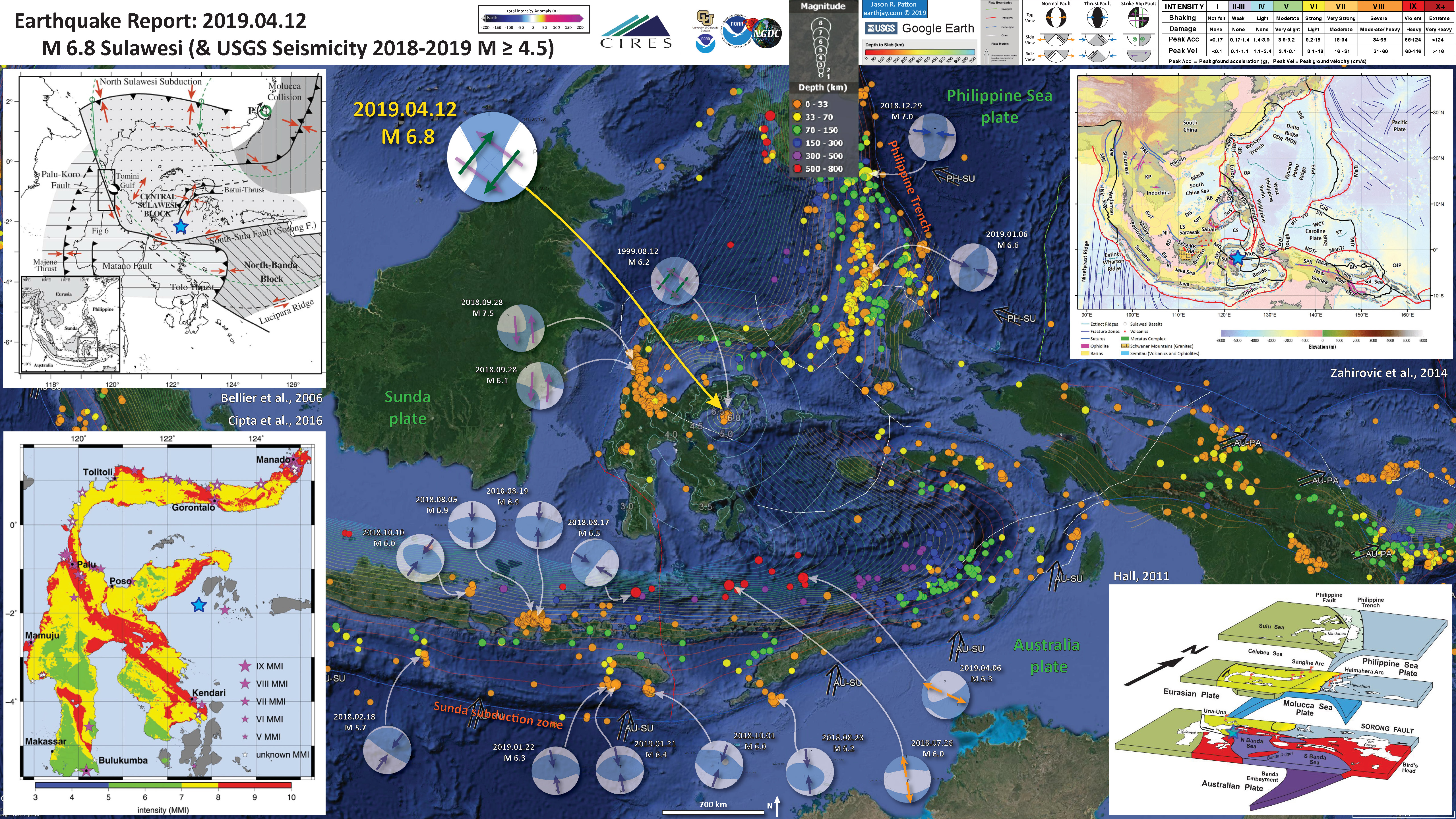
- 2019.04.12 M 6.8 Sulawesi, Indonesia
- Here is the map with a year’s seismicity plotted for quakes M ≥ 4.5.
- Earthquakes from the past year represent well many of the plate boundaries here. Notably is the Donggala/Palu sequence, with all the aftershocks, that align with the trend of the Palu-Koro fault as it connects to the south tot he Sorong fault system.
- There are several quakes along the Java trench (the Sunda subduction zone), showing thrust quakes (e.g. 2.18, 8.28, and 10.1 in 2018 and 1.21 and 1.22 in 2019). The Lombok sequence of 2018 is also evidence of this north-south convergence.
- As the Australia plate dives deep beneath the Sunda plate, the slab (the oceanic crust) pulls downwards, causing extension. The 2018.07.28 M 6.0 and 2019.04.06 normal fault earthquakes (orange arrows) are great examples of this. Intermediate depth earthquakes are not completely understood, but we learn more every year. For example, sometimes there are compressional quakes (thrust/reverse) that happen at these depths, e.g. the 2018.08.17 M 6.5 quake.
- One of the more active regions is the Molucca Strait, where there are subduction/convergent zones that oppose each other. The 2019.01.06 M 6.6 shaker is a good example of what can happen here (and does rather frequently).
- Further north is the subduction zone that forms the Philippine trench. There was a M 7.0 earthquake on 2018.12.29 that shows evidence of the subduction zone megathrust.
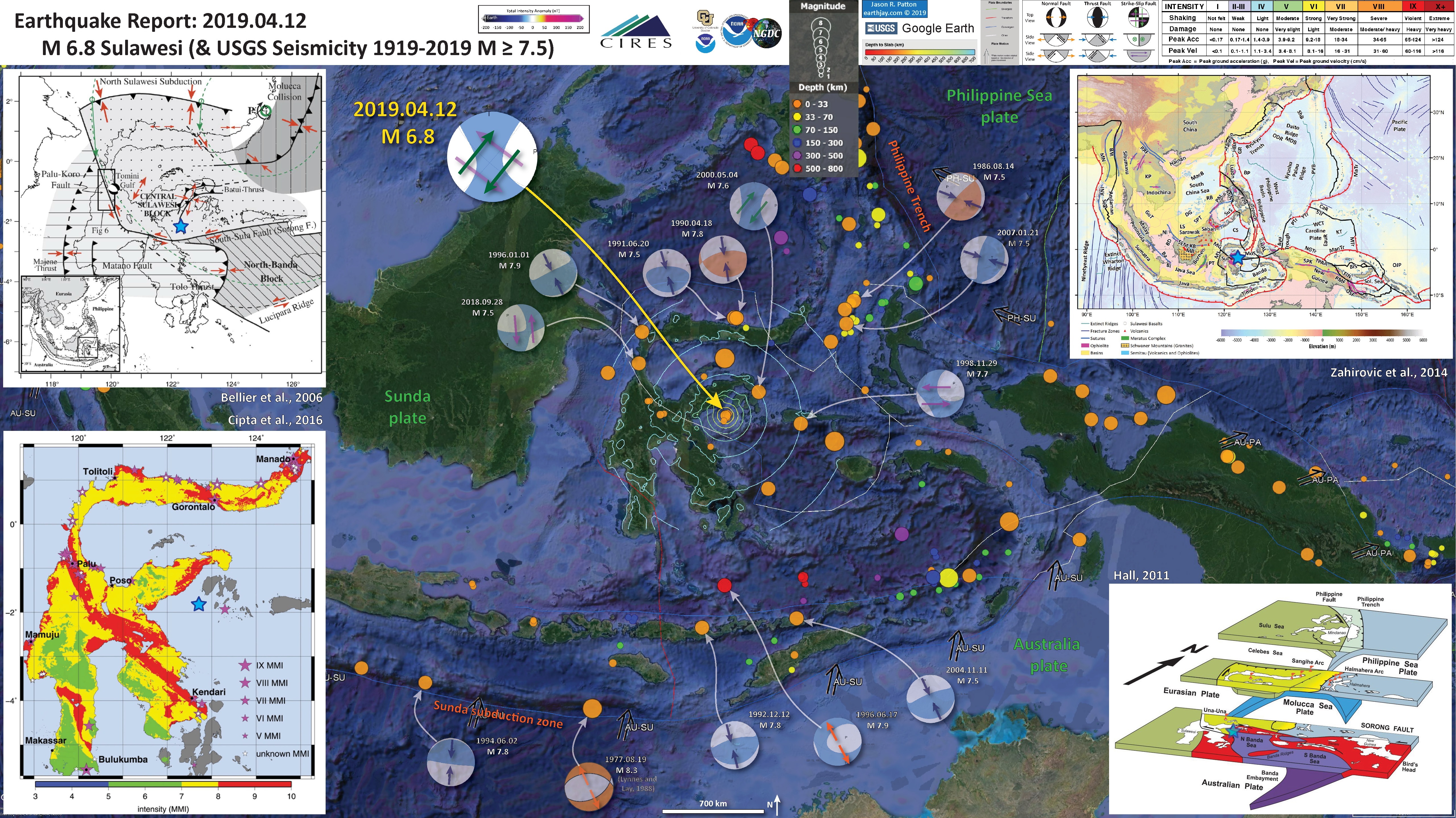
- Here is the map with a century’s seismicity plotted for quakes M ≥ 7.5.
- The USGS earthquake catalog includes additional examples of larger quakes over the past century that represent the range of plate boundary types in the region. The global earthquake catalog is better after 1950 due to the increase in seismic monitoring during the cold war (monitoring for nuclear weapons testing).
- Evidence for subduction along the Sunda subduction zone include subduction zone earthquakes (1977.08.19 M 8.3, 1994.06.02 M 7.8). Also, evidence for down-dip slab-pull extension as evidenced by the 1996.06.17 M 7.9 temblor. similar to the 2018 Lombok sequence, there are also examples of the backthrust to the subduction zone (e.g. 1992.12.12 M 7.8 and 2004.11.11 M 7.5).
- The Molucca Strait thrust earthquakes are evidence for this bivergent convergence (e.g. 1986.08.14 M 7.5 and 2007.01.21 M 7.5).
- There is also a subduction zone on the north side of Sulawesi, with several good example earthquakes (e.g. 1990.04.18 M 7.5, 1991.06.20 M 7.5, and 1996.01.01 M 7.9, which was tsunamigenic).
- There was a strike-slip earthquake on 1998.11.29 that is related to the Sorong fault system, a magnitude M 7.7 shaker.
Today I awoke to the USGS earthquake notification service email about an earthquake offshore of Sulawesi, Indonesia. There was an earthquake with a magnitude M 6.8 to the southeast of the Donggala/Palu earthquake from 28 September 2018. Here is the comprehensive earthquake report for the Donggala/Palu earthquake, landslides, and tsunami.
Just like the September quake, today’s event was a strike-slip earthquake, where the crust moves side-by-side (like the San Andreas fault).
This region of the world is complicated and special. There are subduction zone and transform plate boundaries. I use several maps below to present how these plate boundaries control the types of earthquakes. First I plot the earthquakes from the past year, then for the past century. Of course, let’s remember that seismometers are not that old, so the first half of the 20th century, there were not many seismometers. So, the earthquake record before the 1950s is generally composed of earthquakes with larger magnitude.
There are many many faults in this region, overlapping each other, offsetting each other. And, there have been earthquakes along many of these systems over the past year and past century that represent these different systems and how they interact.
- 2019.05.06 M 7.2 Papua New Guinea
- Here is the map with a century’s seismicity plotted.
Earlier today, there was an intermediate depth beneath eastern Papua New Guinea (PNG). With a magnitude M = 7.2, this is one of the largest earthquake so far in 2019. Here is the USGS website for this earthquake.
Today’s earthquake was quite deep, about 130 km. There are several ways that people have interpreted the tectonics here (which is more common than not).
PNG and New Britain are a region of convergence, where the Australia plate to the south is moving northwards to the Pacific plate (and lots of smaller plates are moving around too).
Today’s M 7.2 temblor is a cool mystery! (see the report for more details)

- 2019.05.12 M 6.1 Panama
- Here is the map with a century’s seismicity plotted.
- Here is the map with the Global Earthquake Model (GEM) strain map as an overlay (Kreemer et al., 2014). Strain is a quantification of the amount of deformation of the Earth over time. Technically, it is the change in shape (length, volume) per unit time. Note how the strain is localized along the subduction zone, as well as along the PFZ.
There was just now an earthquake beneath Panamá. The major plate boundary in the region is a subduction zone (convergent plate boundary) where the Cocos and Nazca plates dive northwards beneath the Caribbean plate forming the Middle America trench (MAT).
This magnitude M = 6.1 earthquake appears to be associated with the transform plate boundary (strike-slip fault) that is formed between the Cocos and Nazca plates. I initially interpreted the earthquake mechanism (e.g. moment tensor) shows this to be a strike-slip earthquake along the Panamá fracture zone (PFZ). However, the earthquake is not currently deep enough according to the USGS Slab 2.0 data (that shows the depth of the megathrust subduction zone, or the top of the downgoing oceanic crust/slab). This is still possible, but it is also possible that this is in the upper plate, the Caribbean plate.


- 2019.05.14 M 7.5 New Ireland
- Here is the map with a century’s seismicity plotted for magnitudes M ≥ 7.5. Because of the complexity of this figure, the magnetic anomaly data are not included.
This region of Earth is one of the most seismically active in the past decade plus. This morning, as I was preparing for work, I got an email notifying me of an earthquake with a magnitude M = 7.5 located near New Ireland, Papua New Guinea.
There are every type of plate boundary fault in this region. There are subduction zones, such as that forms the New Britain and San Cristobal trenches. There are transform faults, such as that responsible for the M 7.5 temblor. There are also spreading ridges, such as the one that forms the Manus Basin to the northwest of today’s quake.
I interpret this M 7.5 earthquake to be a left-lateral strike slip earthquake based on (1) the USGS mechanism (moment tensor), (2) our knowledge of the faulting in the region, and (3) historic analogue earthquake examples. There was an earthquake on a subparallel strike-slip fault on 8 March 2018 (here is the earthquake report for that event). Also in that report, I discuss an earthquake from November 2000 that had a magnitude M = 8.0.

- 2019.05.26 M 8.0 Peru
- Here is the map with a century’s seismicity plotted. Note that I include 2 thrust earthquakes. What are the depths for these temblors? (use the color of the circle to help)
- Here is the map with a century’s seismicity plotted, but also includes the GEM strain data.
Just a moment ago, there was an intermediate depth Great Earthquake (magnitude M≥8.0) beneath Peru. I was heading to bed at about 1:10 local time (Sacramento, CA) when I noticed a tweet from Dr. Anthony Lomax (presenting his first motion mechanism for this earthquake). I realized that I was no longer heading to bed. I put together the interpretive posters and tweeted out to social media, but put off completing the report until today.
The major plate boundary in this region of the world is the subduction zone that forms the Peru-Chile Trench, where the Nazca plate dives eastwards beneath the South America plate.
This magnitude M = 8.0 Great earthquake is extensional (normal) and in the downgoing Nazca plate at a depth of about 110 km. Earthquakes M ≥ 8 are generally considered “Great” earthquakes.


- 2019.06.05 M 4.3 San Clemente Island
- Here is the map with a century’s seismicity plotted.
- Here is a map that shows detailed bathymetry data for the region (Dartnell et al., 2016, 2017) overlain on GEBCO coarser bathymetry data downloaded from GMRT. The land data are at 10 m resolution from The National Map (NED).
- I plot USGS Quaternary Fault and Fold Database faults as faint white lines. Earthquakes include the past month for magnitudes M ≥ 0.5 and events since 1919 for M ≥ 4.0.
- Look at the bathymetry surrounding the island. We can clearly see the SCF to the east of the island. There is evidence for a north-south striking fault to the west of the island. In the area just southeast of the earthquakes, there appears bedrock sticking up out of the continental shelf. This bedrock aligns with a ridge in the slop to the south of the island. This ridge may just be sediment, but it may also be tectonic in origin.
- Here is a larger scale map so that we can look at the bathymetry surrounding San Clemente Island in greater detail. I updated the USGS seismicity for 2019.06.06 at 20:00 Pacific time.
- Here is a map I prepared using the 2016 USGS Topobathy data (LiDAR and historic bathymetry mosaic).
- I present these data as a shaded relief (hillshade) beneath an elevation raster with color representing height or depth. I also use a slopeshade raster to help highlight the changes in slope.
- The 100 meter topographic contours are labeled. The inset shows the location of the main map in relation to the CCB with a pink polygon.
Well, yesterday was the start of a sequence of earthquakes offshore of San Clemente Island, about 100 km west of San Diego, California. The primary tectonic player in southern CA is the Pacific – North America plate boundary fault, the San Andreas (SAF).
The region offshore where this ongoing sequence is called the California Continental Borderlands (CCB). There exists an excellent record of how the North America – Pacific plate margin boundary has evolved through time (remember, prior to about 29 million years ago, this plate boundary in southern CA was a subduction zone).
There was an earthquake offshore of Los Angeles last year. Check out my earthquake report and report update.
In places the SAF is a single thoroughgoing fault (e.g. in the southern San Joaquin Valley), in others it splays into multiple strands (in Orange County between the Santa Ana Mtns and Lake Elsinore), and in other places it bends to create regions of uplift (like in Ventura or the Santa Monica Mtns). The active faulting in the CCB is basically a series of right-lateral faults that step and bend to form uplifted islands and terraces, along with pull-apart sedimentary basins.
San Clemente Island is a region of uplifted non-marine Tertiary volcanic rocks (andesite and dacite) with ages ranging from 14.8 – 16.5 million years ago (Yeats, 1968; Merifield et al., 1971; Ward and Valenise, 1996). These rocks are overlain by Tertiary (Miocene) sediments (limestone, siltstone, shale, and diatomite; correlates to the Monterey Formation) and Plio-Pleistocene sediments (sandstones and conglomerates; correlates to the Fernando Formation found onshore; Stadum & Susuki, 1976; Ward and Valenise, 1996).
Muhs et al. (2014) used numerical ages (uranium-series analysis of corrals and amino acid geochronology of mollusks) to calculate marine terrace uplift rates in the CCB. When compared to uplift rates from different tectonic regimes, the terrace uplift rates in CCB is comparable to regions where strike-slip tectonics are dominant. These authors suggest that uplift like that found at the Big Bend (e.g. Ventura and Santa Monica Mtns) is not influencing terrace uplift rates in the CCB.
Along with this compression, there is a right-lateral (dextral) strike-slip fault on the east side of the island, the San Clemente fault, which has a slip rate of about 1 – 4 mm.yr (Ward and Valensise, 1996). The Southern California Earthquake Center suggests the slip rate is about 1.5 mm/yr for the SCF.
The ongoing sequence of earthquakes near the San Clemente Island are small in magnitude. If these were foreshocks to a larger earthquake, this would be felt across the southland, possibly cause damage on the island (where there is a U.S. Naval base), could possibly trigger submarine landslides or a small tsunami. Strike-slip earthquakes are not always considered a significant source for large tsunami, but there is abundant evidence that they do, though often much smaller than tsunami generated from thrust or subduction zone earthquakes. It is possible, if not probable, that this sequence will fizzle out.


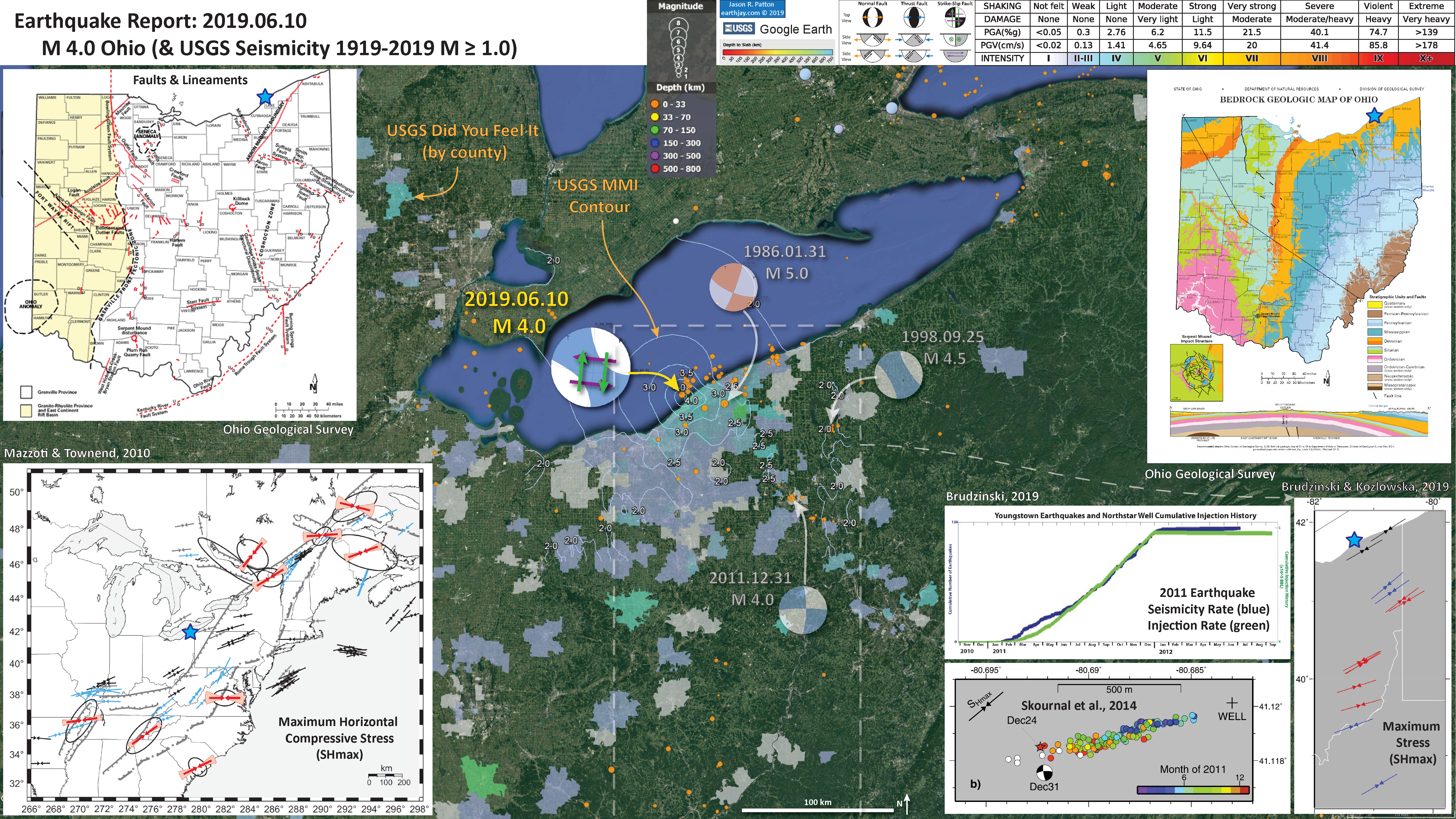
- 2019.06.10 M 4.0 Ohio
https://earthquake.usgs.gov/earthquakes/eventpage/us70003xny/executive
- 2019.06.14 M 6.4 Chile
- Here is the map with a seismicity plotted that is associated with specific earthquakes. I plot earthquakes for the 3 months following the mainshock listed for these example earthquakes (e.g. 1960, 1985, 2007, 2014, and 2015.
This morning (my time) there was a magnitude M 6.4 earthquake offshore of Chile. While it was in the correct location to possibly cause a tsunami, the magnitude was too small.
The major plate boundary here is the megathrust subduction zone that forms the Peru-Chile trench. Here, the Nazca plate dives eastwards beneath the South America plate.
Many people are familiar with subduction zone earthquakes which are responsible for the largest size temblors possible, as well as tsunami capable of travelling across the entire Pacific Ocean. The largest earthquake recorded on modern instruments is the 22 May 1960 M 9.5 Chile earthquake. There have been 2 large transoceanic tsunami caused by subduction zone earthquakes in 2010 and 2015. At the bottom of this report is a list of other earthquakes in this region.

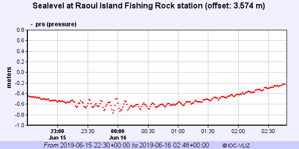
- 2019.06.15 M 7.2 Kermadec
- These are the tide gage data from Raoul Island.
- These are data from 15 Jun 22:30 UTC until 16 Jun 02:48 UTC.
- Here is the map with a month’s seismicity M ≥ 0.5 plotted (and magnetic anomalies).
- Here is the map with a century’s seismicity M ≥ 6.0 plotted (and strain).
There was just an earthquake associated with the plate boundary that forms the Kermadec Trench, a deep oceanic trench that extends north from New Zealand, towards the Fiji Islands.
A minor tsunami (~25 cm in size) has been recorded at Raoul Island, due west of the earthquake, the closest gage to the temblor. Tide gages in New Zealand just began recording a small tsunami the moments I started writing this report (about an hour ± after the earthquake).
In this part of the world, there is a convergent plate boundary where the Pacific plate dives westward beneath the Australia plate forming the Kermadec megathrust subduction zone fault. This fault has a history of earthquakes with magnitudes commonly exceeding M 7 and some exceeding M 8.
- 2019.06.23 M 5.6 Petrolia
- Here is the map with a month’s seismicity plotted.
- Here is the map with a century’s seismicity plotted along with the Global Strain Map with a 30% transparency.
Well, I was on the road for 1.5 days (work party for the Community Village at the Oregon Country Fair). As I was driving home, there was a magnitude M 5.6 earthquake in coastal northern California.
This earthquake follows a sequence of quakes further to the northwest, however their timing is merely a coincidence. Let me repeat this. The M 5.6 earthquake is not related to the sequence of earthquakes along the Blanco fracture zone.
This region also had a good sized shaker in 1992, the Cape Mendocino Earthquake, which led to the development of the National Tsunami Hazard Mitigation Program. More about the Cape Mendocino Earthquake can be found on the 25th anniversary page here and in my earthquake report here.
The regional tectonics in coastal northern California are dominated by the Pacific-North America plate boundary. North of Cape Mendocino, this plate boundary is convergent and forms the Cascadia subduction zone (CSZ). To the south of Cape Mendocino, the plate boundary is the right-lateral (dextral) San Andreas fault (SAF). Where these 2 fault systems meet, there is another plate boundary system, the right-lateral strike-slip Mendocino fault (don’t write Mendocino fracture zone on your maps!). Where these 3 systems meet is called the Mendocino triple junction (MTJ).
Last night’s M 5.6 temblor happened where one strand of the MF trends onshore (another strand bends towards the south). But, it also is where the SAF trends onshore. At this point, I am associating this earthquake with the MF (so, a right-lateral strike-slip earthquake). The mechanism suggest that this is not a SAF related earthquake. However, it is oriented in a way that it could be in the Gorda plate (making it a left-lateral strike-slip earthquake). However, this quake is at the southern edge of the Gorda plate (sedge), so it is unlikely this is a Gorda plate event.

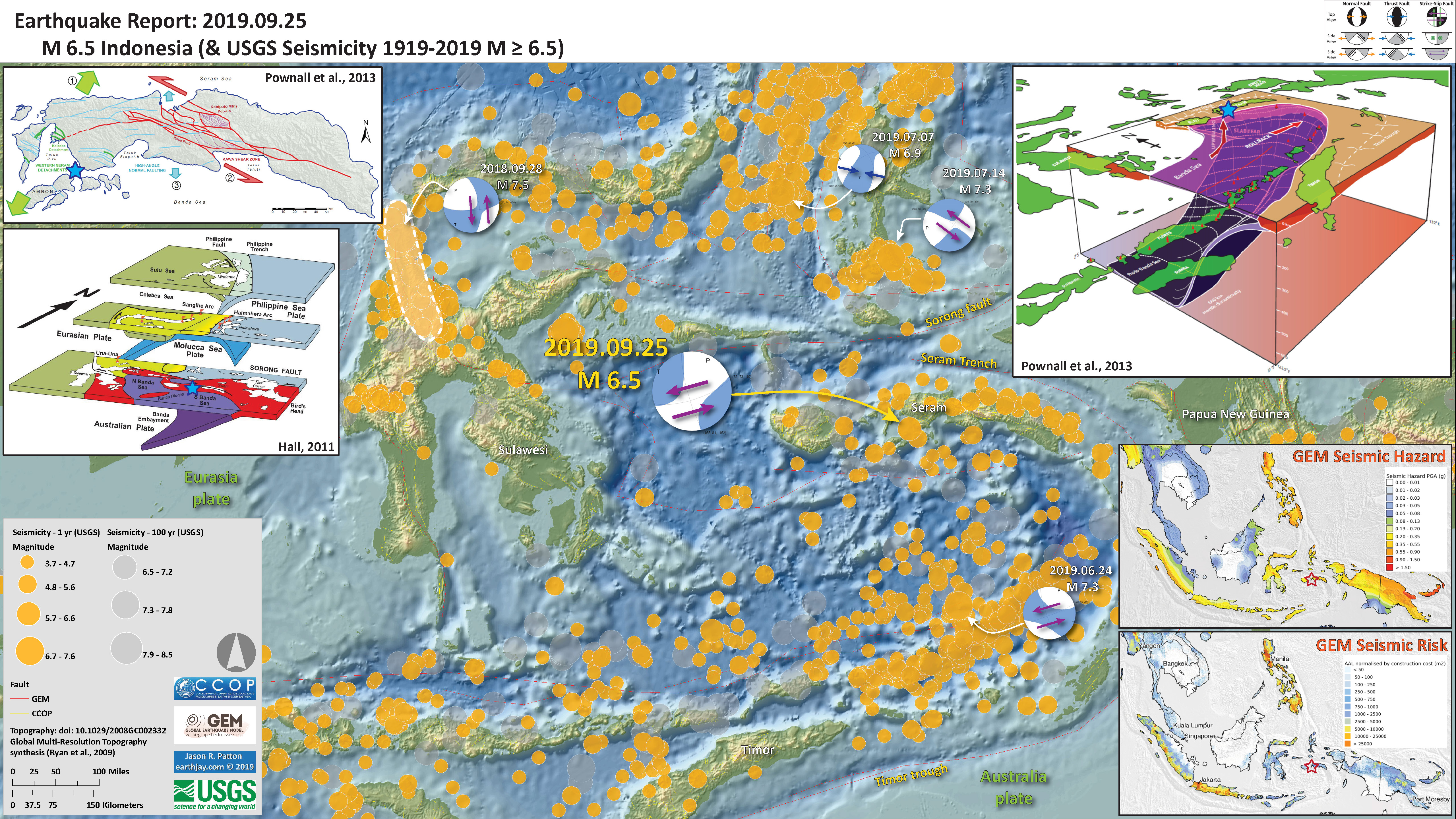
- 2019.06.23 M 7.3 Banda Sea
- Here is the map with a month’s seismicity plotted. I included MMI contours from a recent M 6.3 earthquake in PNG, which led to a sequence of additional M~6 quakes to the southeast of that main shock. I won’t be writing a report for those quakes, even though it is interesting (check it out!). Sorry to have misspelled Hengesh as Hangesh.
- Here is the map with a century’s seismicity (M ≥ 7.0) plotted.
- Here is the map with a month’s seismicity (M ≥ 0.5) plotted with the Global Strain data plotted. We can see the 2018 Flores swarm show up here.
I had been making an update to an earthquake report on a regionally experienced M 5.6 earthquake from coastal northern California when I noticed that there was a M 7.3 earthquake in eastern Indonesia.
This earthquake is in a region of strike-slip faulting (if in downgoing plate for example) or subduction thrusting, so I thought it may or may not produce a tsunami. There are also intermediate depth quakes here (deeper than subduction zone megathrust events), like this earthquake (which reduces the chance of a tsunami). While we often don’t think of strike-slip earthquakes as those that could cause a tsunami, they can trigger tsunami, albeit smaller in size than those from subduction zone earthquakes or locally for landslides. But, I checked tsunami.gov just in case (result = no tsunami locally nor regionally). I also took a look at the tide gages in the region here and here (result = no observations).


- 2019.06.25 M 6.2 Panama
https://earthquake.usgs.gov/earthquakes/eventpage/us7000455l/executive
- 2019.07.04 M 6.4 Ridgecrest
- Here is the map with a century’s seismicity plotted, for quakes M ≥ 5.0.
- Here is the map with a century’s seismicity plotted, for quakes M ≥ 5.0 with the Global Strain Map as an overlay.
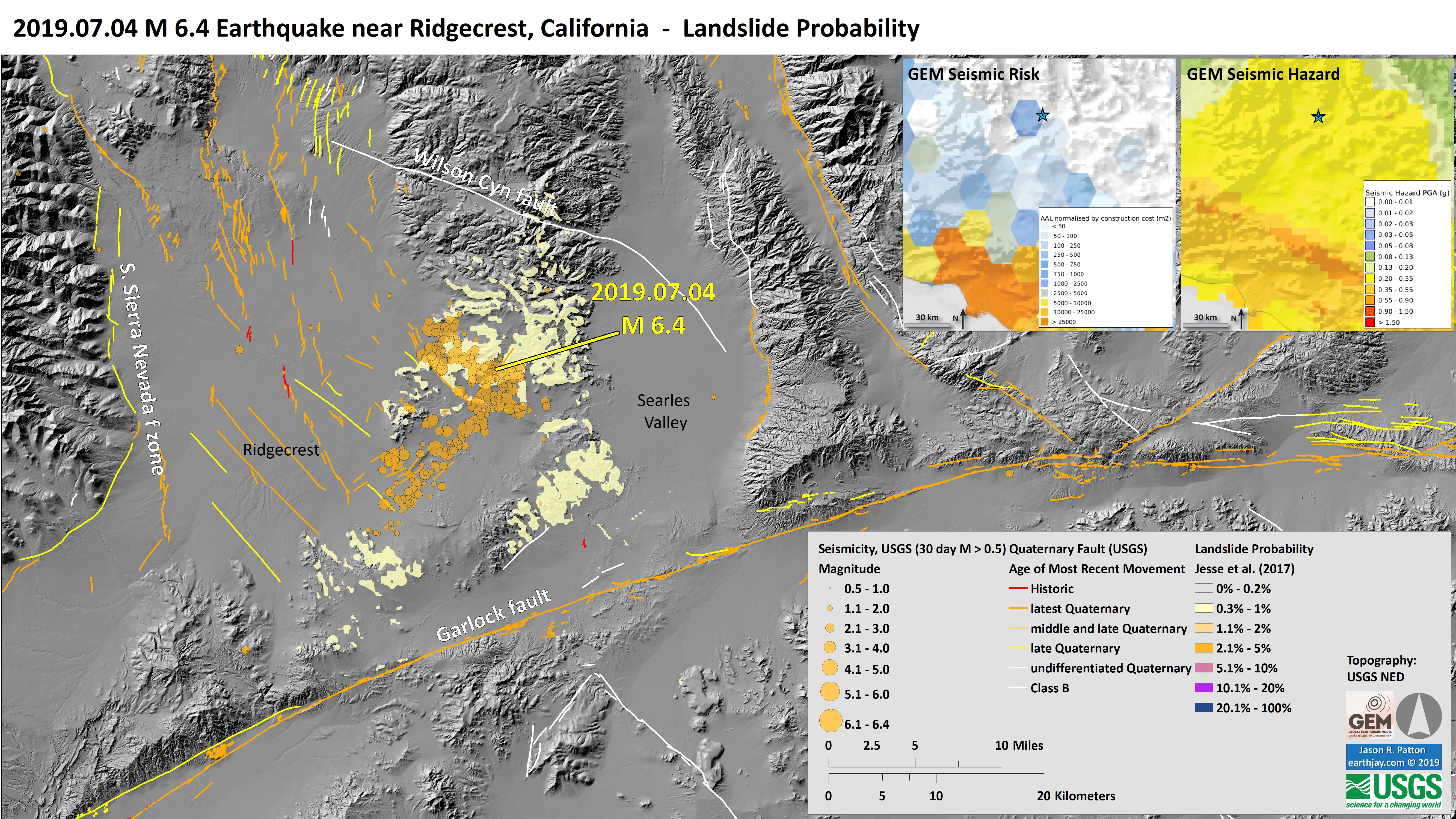
- Here is a suite of maps that use USGS earthquake products to help us learn about how earthquakes may affect the landscape: landslide probability and liquefaction susceptibility (a.k.a. the Ground Failure data products)..
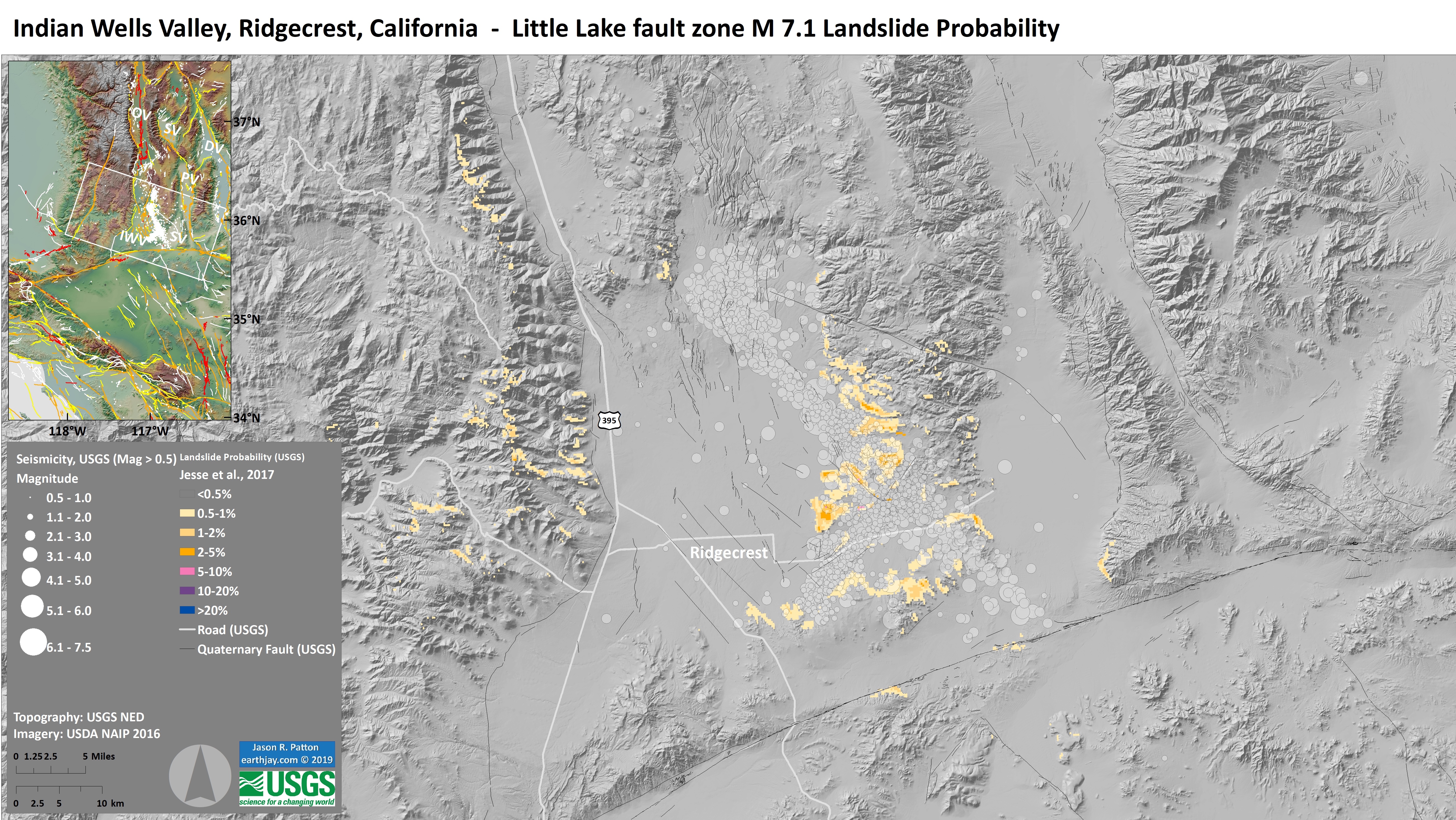
- First I present the landslide probability model. This is a GIS data product that relates a variety of factors to the probability (the chance of) landslides as triggered by this earthquake. There are a number of assumptions that are made in order to be able to produce this model across such a large region, though this is still of great value (like other aspects from the USGS, e.g. the PAGER alert). Learn more about all of these Ground Failure products here.
- I use the same color scheme that is presented by the USGS on their website. Note that the majority of areas that may have experienced earthquake triggered landslides are cream in color (0.3-1%). There are a few places with a slightly higher chance that there were triggered landslides. It is possible that there were no significant landslides from this earthquake. The lower bounds for earthquake triggered landslides on land is about M 5.5 and a M 6.4 releases much more energy than that.
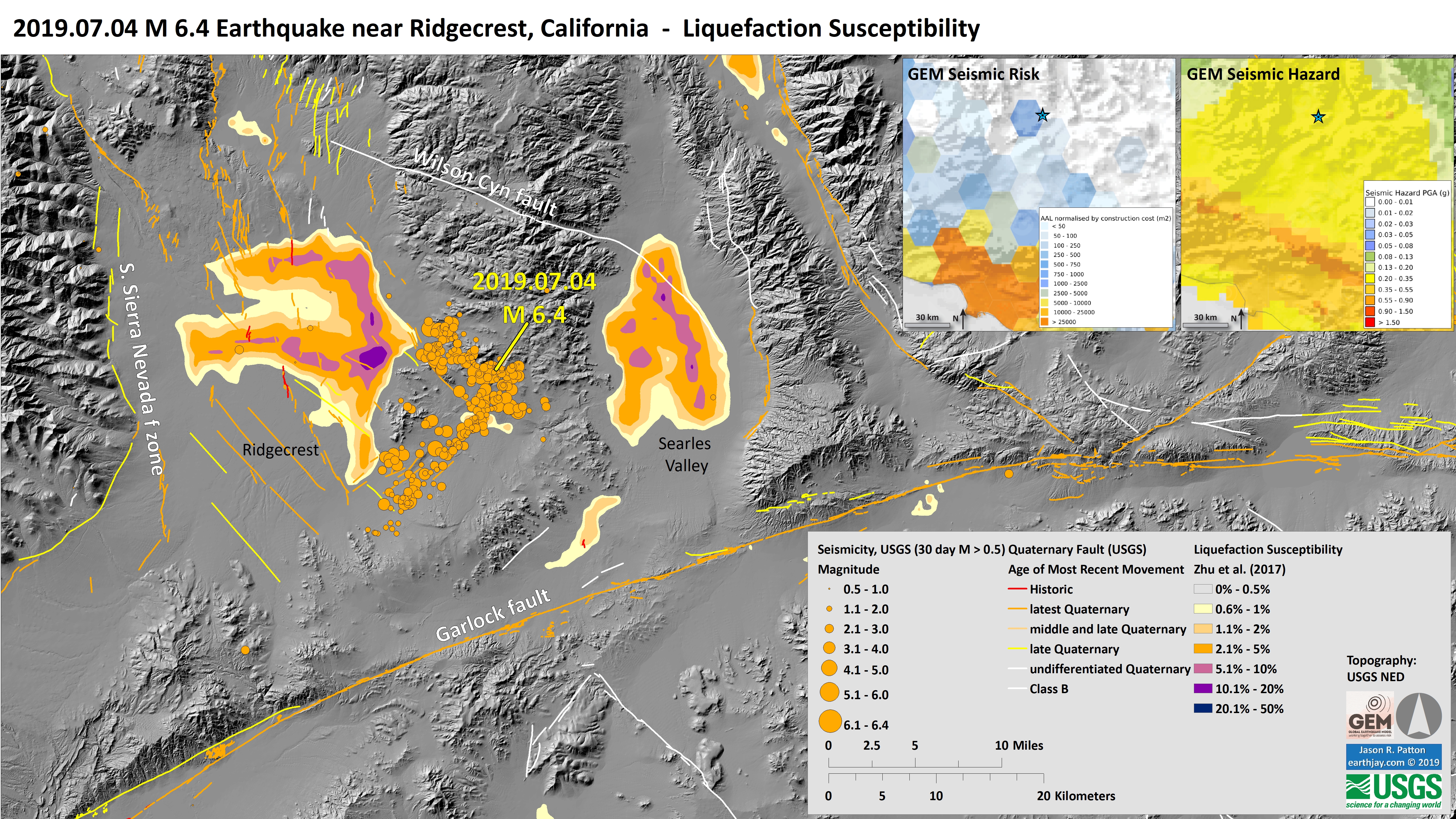
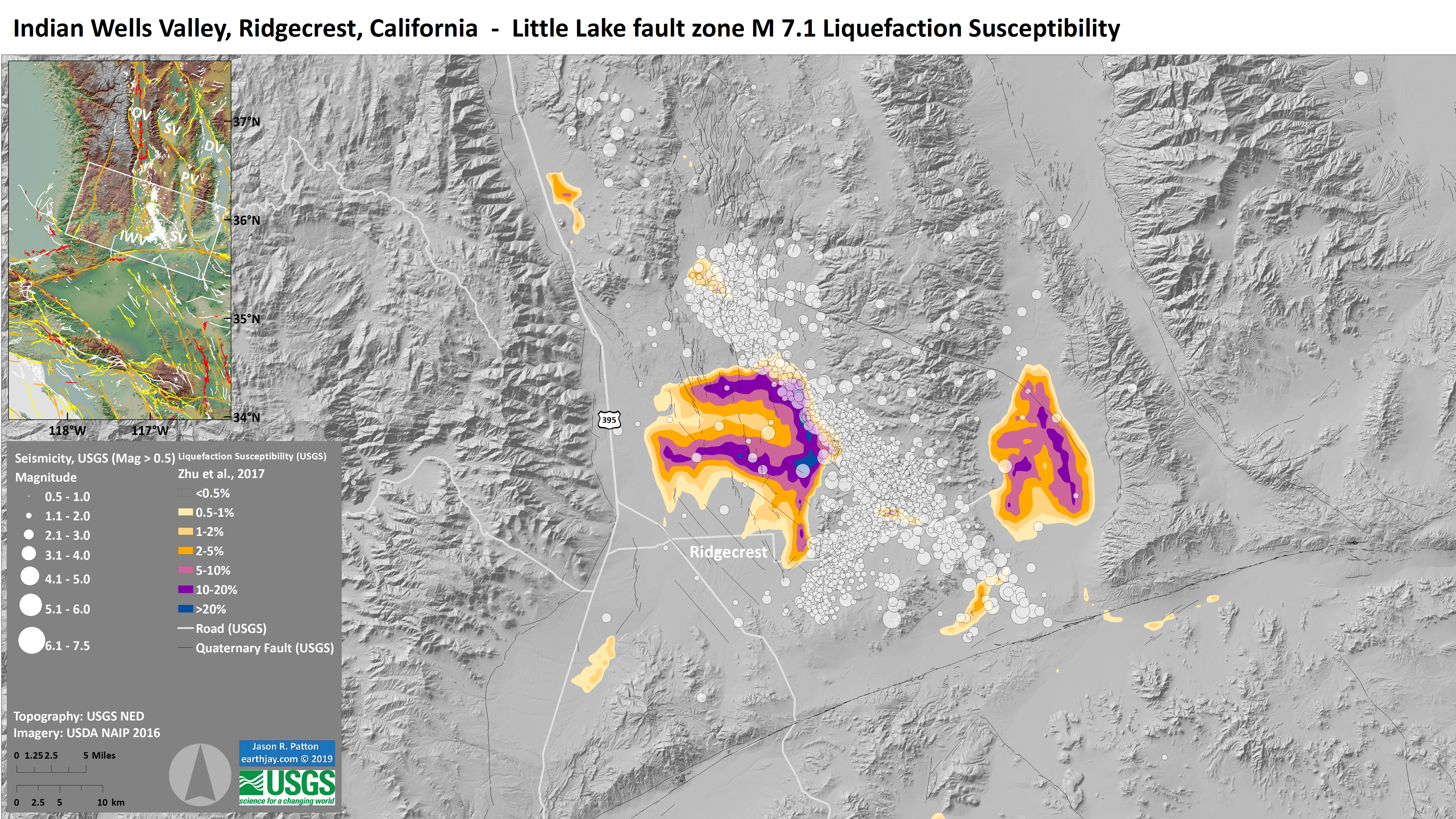
- Sediment or soil strength is based upon the ability for sediment particles to push against each other without moving. This is a combination of friction and the forces exerted between these particles. This is loosely what we call the “angle of internal friction.” Liquefaction is a process by which pore pressure increases cause water to push out against the sediment particles so that they are no longer touching.
- An analogy that some may be familiar with relates to a visit to the beach. When one is walking on the wet sand near the shoreline, the sand may hold the weight of our body generally pretty well. However, if we stop and vibrate our feet back and forth, this causes pore pressure to increase and we sink into the sand as the sand liquefies. Or, at least our feet sink into the sand.
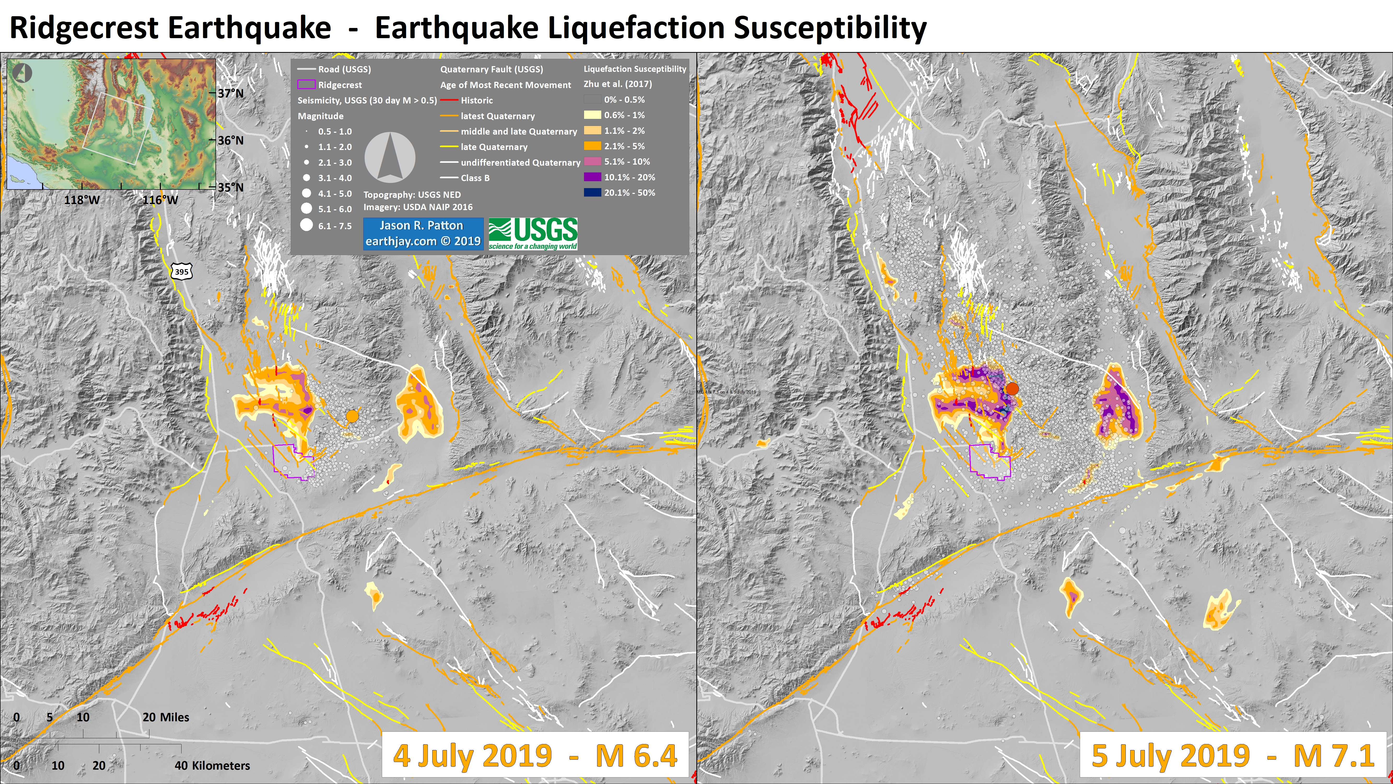
- Below is the liquefaction susceptibility map. I discuss liquefaction more in my earthquake report on the 28 September 20018 Sulawesi, Indonesia earthquake, landslide, and tsunami here.
- I use the same color scheme that the USGS uses on their website. Note how the areas that are more likely to have experienced earthquake induced liquefaction are in the valleys. The fact that this earthquake happened in the summer time suggests that there may not have been any liquefaction from this earthquake.
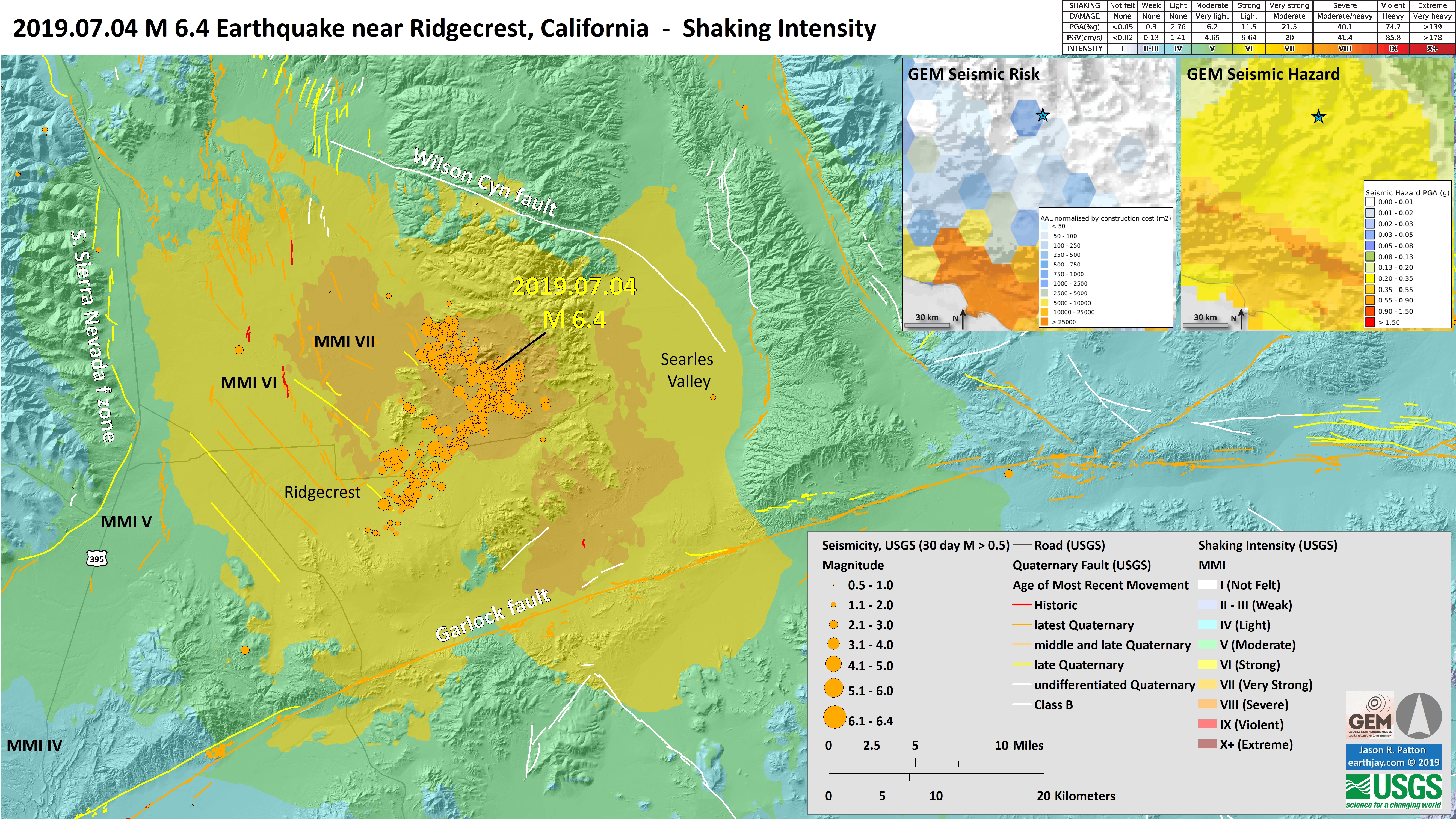
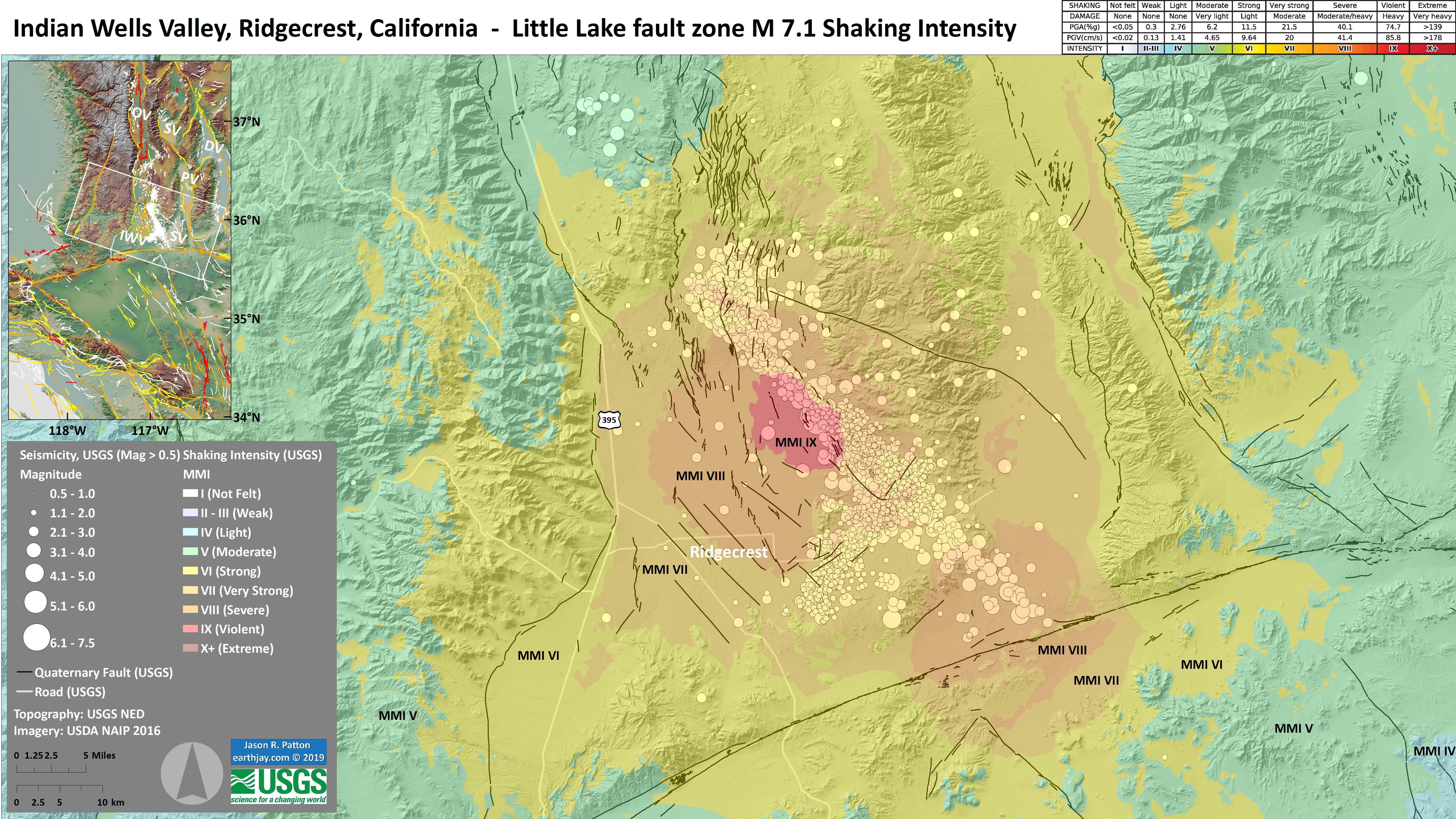
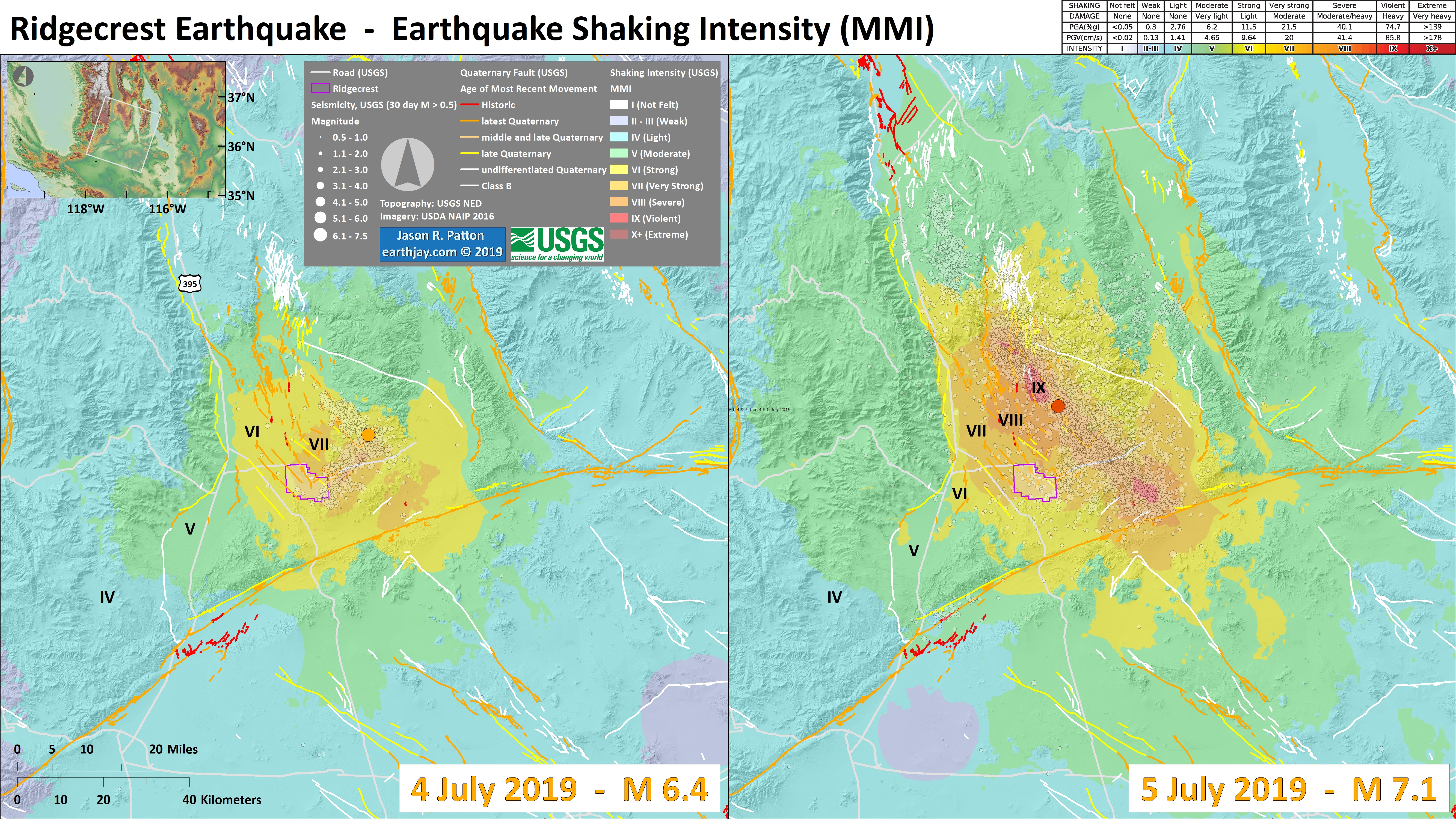
- Finally, here is a map showing the earthquake shaking intensity. The scale is the Modified Mercalli Intensity scale (explained above).
- I also include two inset maps (also in the landslide and liquefaction maps). These are seismic hazard and seismic risk maps. Read more about these maps here.
- On the right is the Global Earthquake Model Seismic Hazard map. Color represents the amount of shaking that an area may experience over the next 50 years. The units are “g” (which stands for gravity, where g= 1 is the gravity at the Earth’s surface). If g > 1, objects can be thrown into the air.
- On the left is the GEM Seismic Risk map. Risk is the combination of hazard and people. If there is seismic hazard where there are no people, then there is no seismic risk. If there are people where there is no seismic hazard, there is no seismic risk. Seismic risk happens when there are people exposed to seismic hazard. The color represents the financial expense due to seismic hazards.
- 2019.07.05 M 6.4 / 7.1 Ridgecrest Update #1
- Here is an updated map. Please see previous maps and reports for more information about what is on this map.
- I have plotted epicenters from the past few days for magnitudes M > 0.5 in green and earthquakes for the past century for magnitudes M > 5.0.
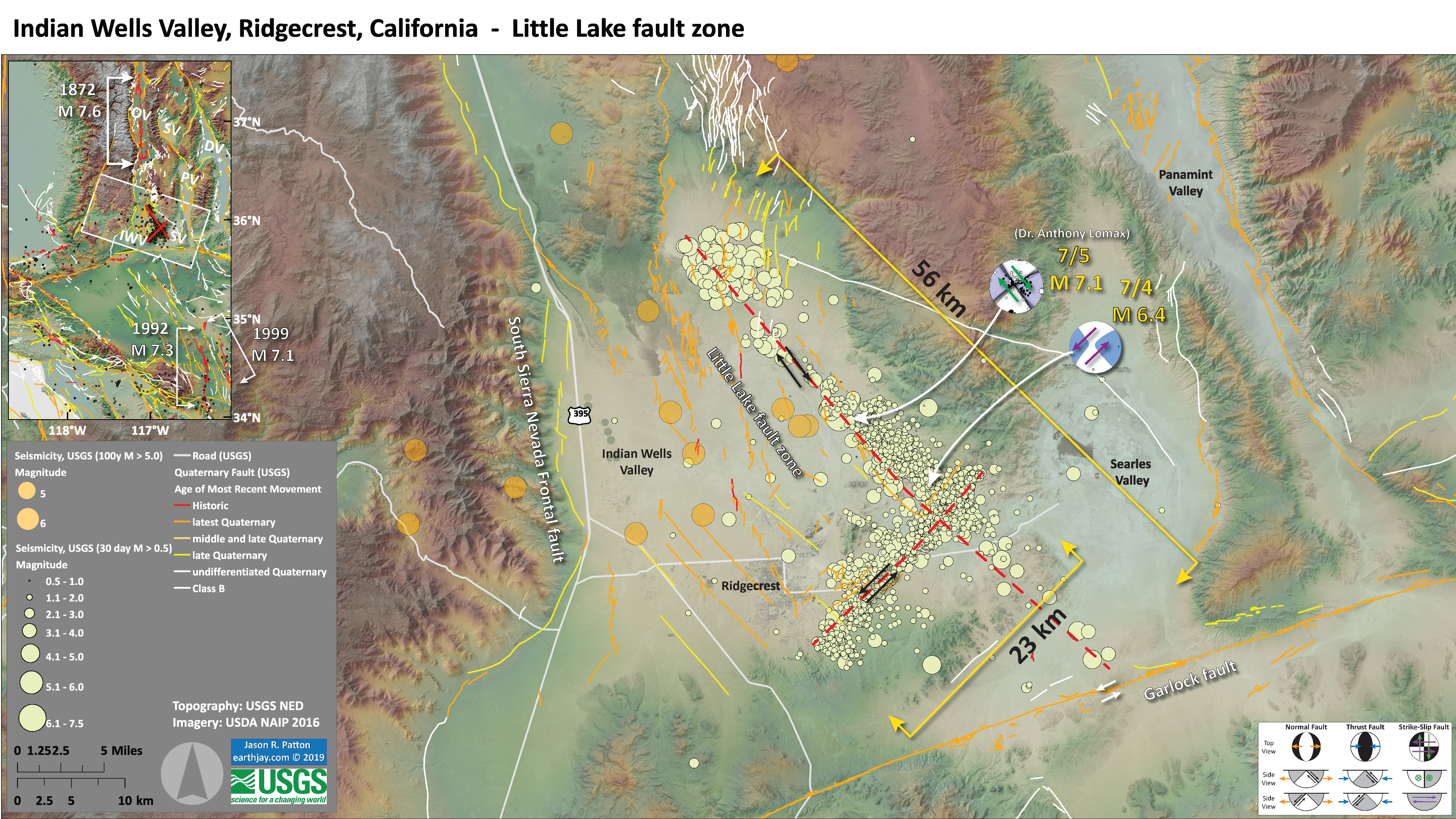
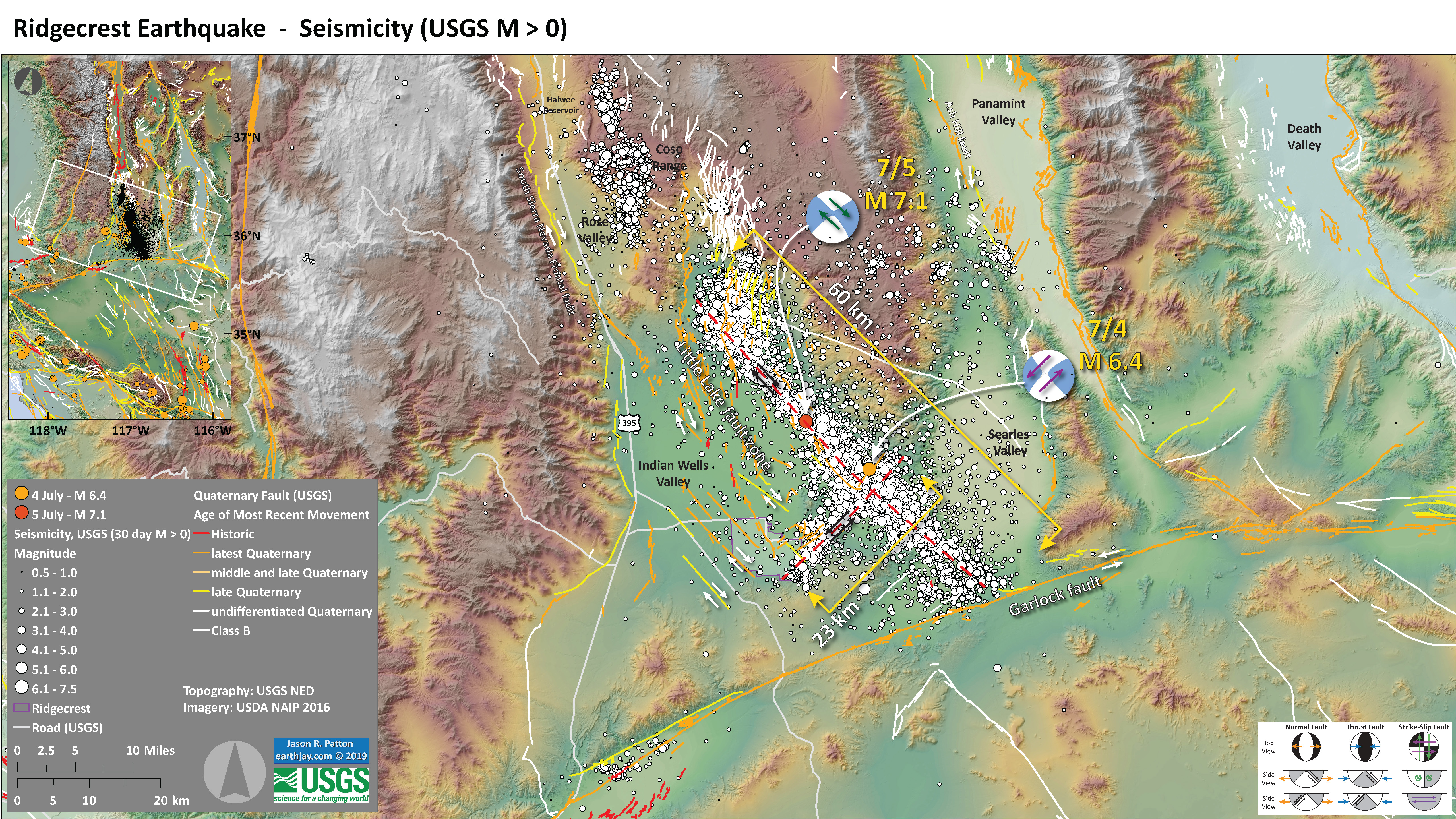
- As I have discussed earlier and here, there are 2 major faults that are participating in this sequence. One fault is a northeast striking (oriented) left-lateral strike-slip fault (analog = Garlock fault). The other fault is a northwest striking (oriented) right-lateral strike-slip fault (analog = San Andreas, Owens Valley faults). There are also many other smaller faults too.
- Earlier I interpreted the M 6.4 to have been on the northeast striking left-lateral strike-slip fault. This is still my favored interpretation as (1) using the empirical fault scaling relations from Wells and Coppersmith (1995), the 23 km length could produce a magnitude M 6.6 earthquake (close enough to > 6.4), (2) this is where the aftershocks were following the M 6.4, and (3) the surface rupture was identified along the northeast striking region. However, it may be on the northwest striking fault.
- The M 7.1 earthquake is clearly on the nw striking right-lateral strike-slip fault. The aftershocks are filling in, showing us the spatial extent (the length) of this fault rupture. At first, there were several M 4+ aftershocks at the northwestern end of the aftershocks. As I was preparing the map below, some starting ripping off to the southeast of the ne striking fault. The nw fault appears to be about 60 km long. Using Wells and Coppersmith, a 56 km long rupture would produce a M 7.0 magnitude earthquake. Imagine that!
- Here are some updated maps. I am heading to the field tomorrow, so probably won’t be providing more updates, but we will see.
- Here is an updated seismicity map. The aftershock zone is now extending all the way to the Garlock fault. Also, there are some triggered events far to the northwest of the aftershock zone. These are probably not part of the main northwest trending fault, which appears to end near where the aftershocks are. The pdf version of this map is 167 MB.
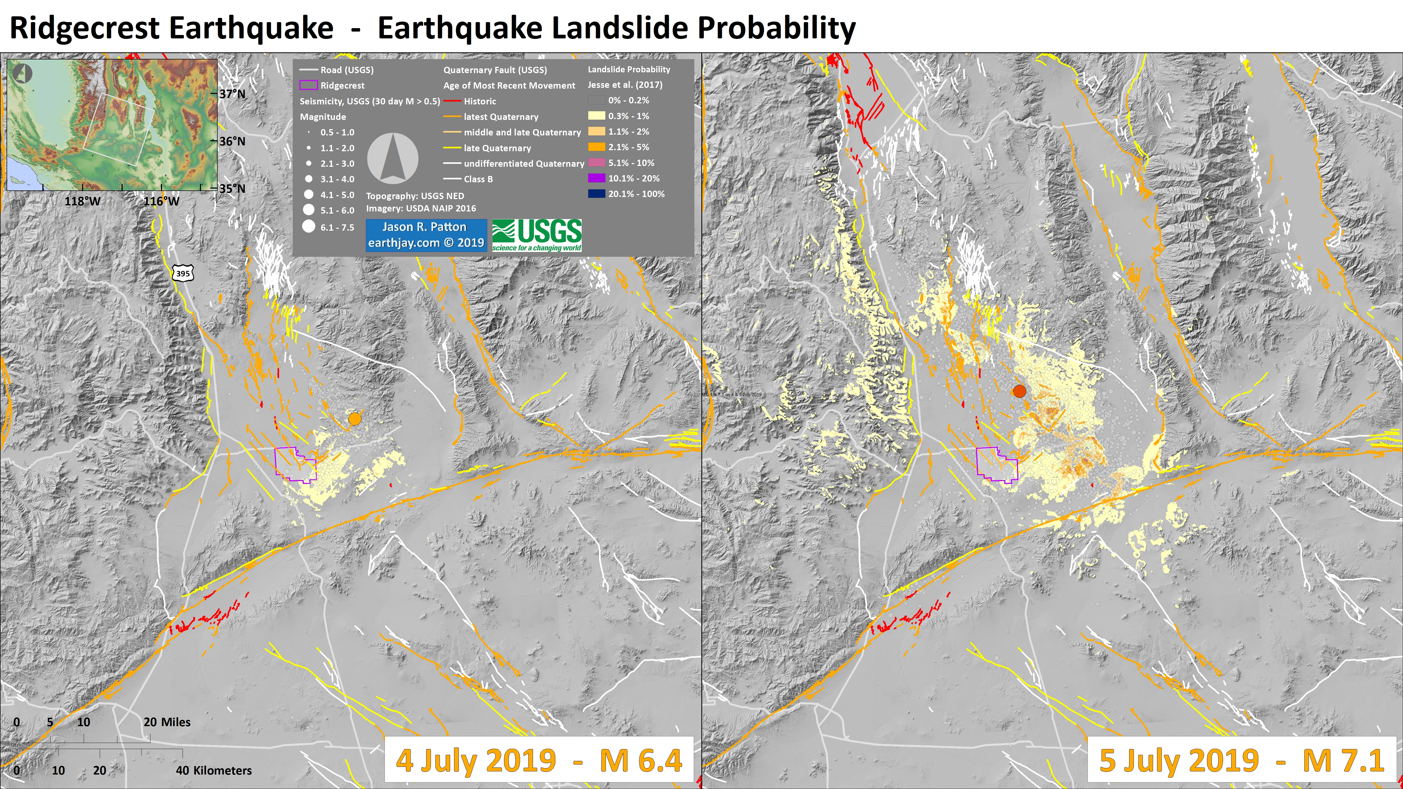
- Here is a map with landslide probability on it. I prepared one like this for the M 6.4 earthquake. Please head over to that report for more information about the USGS Ground Failure products (landslides and liquefaction). Basically, earthquakes shake the ground and this ground shaking can cause landslides. We can see that there is a low probability for landslides. However, we have already seen photographic evidence for landslides and the lower limit for earthquake triggered landslides is magnitude M 5.5 (from Keefer 1984-ish).
- Here is a map showing liquefaction susceptibility. I explain more about this type of map in my original report for the M 6.4 earthquake. Scroll down a bit to find the landslide and liquefaction maps for that event.
- Finally, here is a map that shows the shaking intensity for the M 7.1 earthquake. As I mention in my original report, this is based on a model that relates earthquake shaking intensity with earthquake magnitude and distance from the earthquake. Note that there was violent shaking from the M 7.1 event (MMI IX).
- 2019.07.18 M 6.4 / 7.1 Ridgecrest Update #2
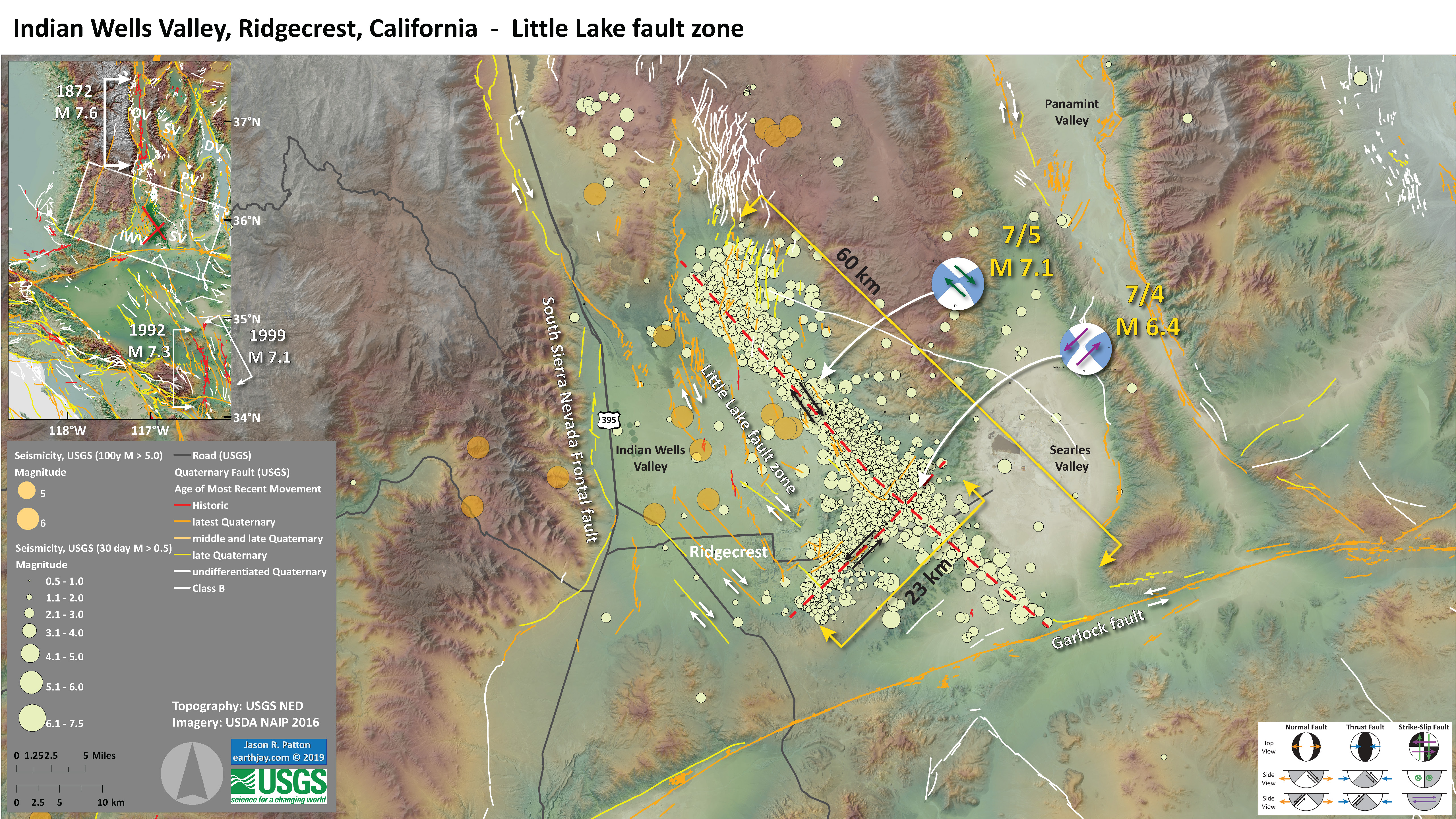
- Here is an updated seismicity map. There are two main types of earthquakes on this map. I present this map both with aerial imagery and with a topographic (“hillshade”) basemap. I outline the general area of Ridgecrest in purple.
- First, there are an abundance of aftershocks aligned with the two main faults that ruptured during this sequence (the northwest trending M 7.1 fault and the northeast trending M 6.4 fault). Part of the northwest striking fault ruptured during the M 6.4 event.
- Second, there are several areas that show earthquakes that were triggered by this sequence. There are some triggered earthquakes along the Coso Range (where the Coso Geothermal Field is located), some events along the Garlock fault, and some temblors along the Ash Hill fault (in Panamint Valley, to the north of Searles Valley).
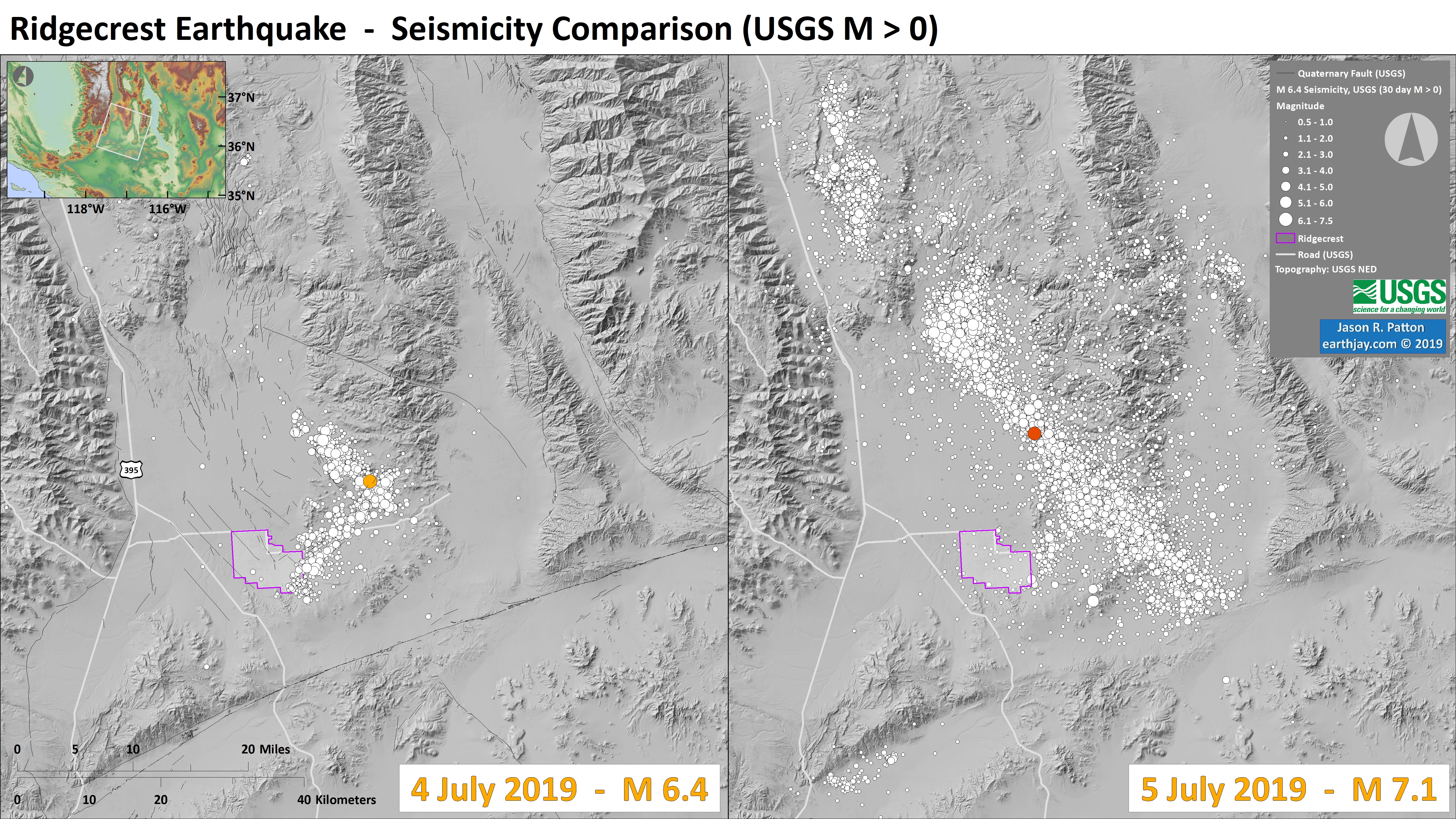
- This is a seismicity comparison for the two earthquakes. on the left are earthquakes (USGS) from prior to the M 7.1 earthquake and on the right are quakes after and including the M 7.1 temblor. I plot the USGS Quaternary fault and fold database on the left as black lines.
- Here is a map with landslide probability on it. Please head over to that report for more information about the USGS Ground Failure products (landslides and liquefaction). Basically, earthquakes shake the ground and this ground shaking can cause landslides. We can see that there is a low probability for landslides. However, we have already seen photographic evidence for landslides and the lower limit for earthquake triggered landslides is magnitude M 5.5 (from Keefer 1984-ish).
- Here is a map showing liquefaction susceptibility. I explain more about this type of map in my original report for the M 6.4 earthquake. Scroll down a bit to find the landslide and liquefaction maps for that event.
- Finally, here is a map that shows the shaking intensity for the M 6.4 and M 7.1 earthquakes. As I mention in my original report, this is based on a model that relates earthquake shaking intensity with earthquake magnitude and distance from the earthquake. Note that there was violent shaking from the M 7.1 event (MMI IX).
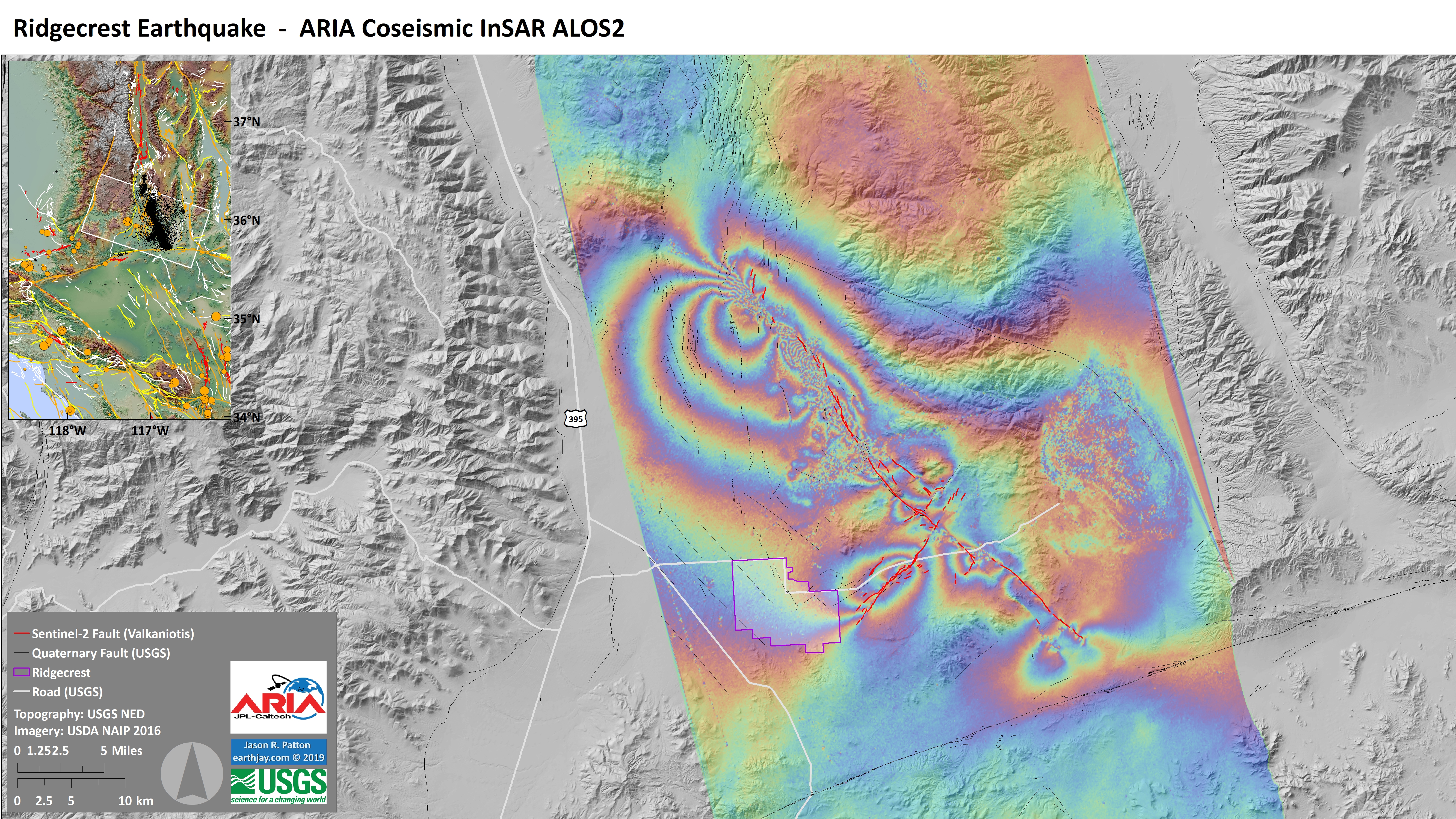
- NASA Jet Propulsion Laboratory (JPL) prepares Advanced Rapid Imaging and Analysis (ARIA) data products for major events worldwide. Their data are presented online here. I used the data from this event in a GIS computer program, but the data are prepared in Google Earth files too (so everyone can use them if they have a modern computer with an internet connection). This is a valuable government service.
- This first map shows the results of modeling Synthetic Aperture Radar Interferometry data. Basically, Radar satellite imagery data from before and from after the earthquake are compared to model the amount of ground deformation that occurred between the satellite acquisitions. Each color band represents a certain amount of motion. This is referred to as the wrapped image.
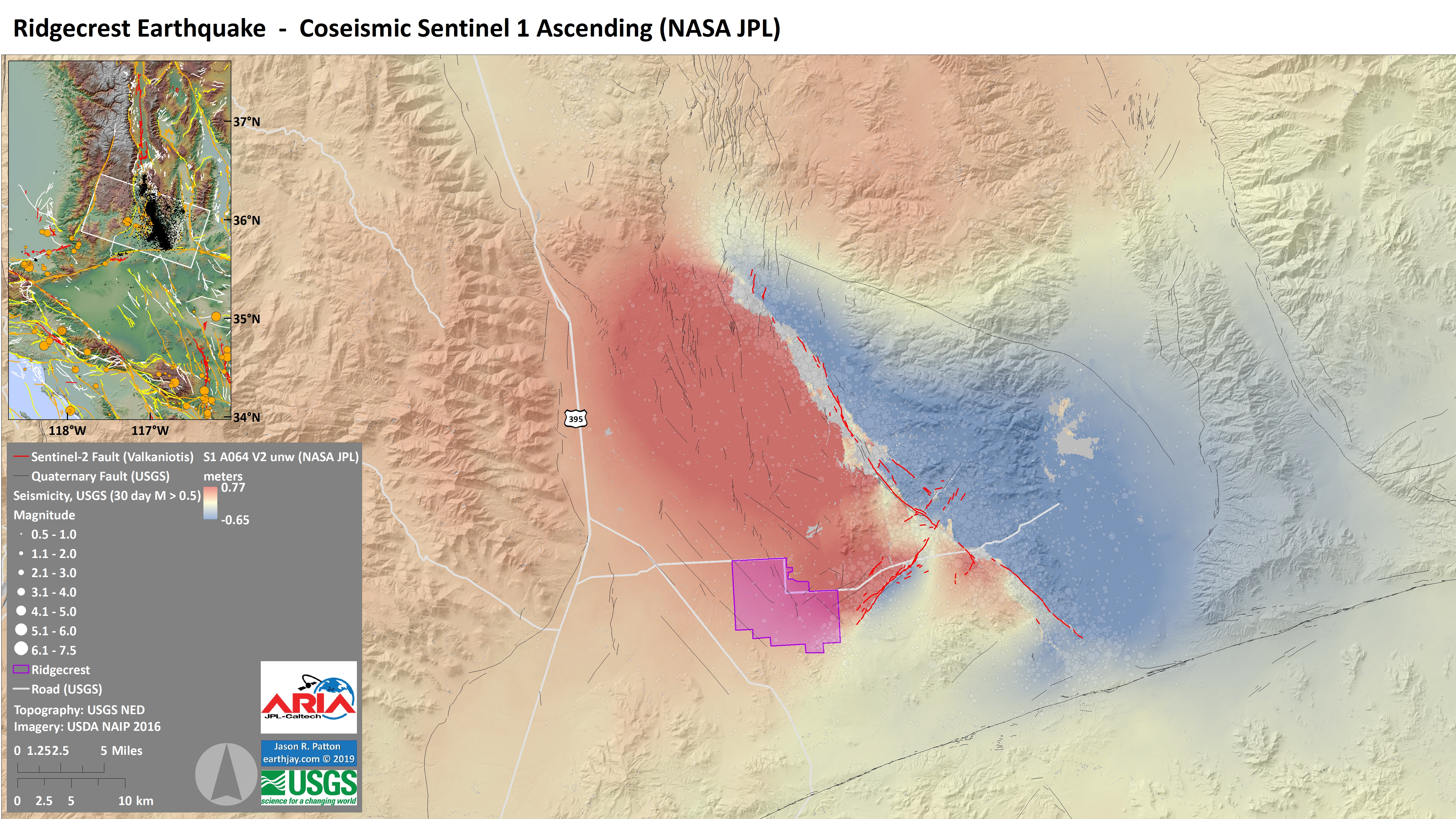
- This map is made using the same basic data, though it has been processed in a way to show the overall ground motion with just two colors, instead of color bands. This is called the unwrapped image.
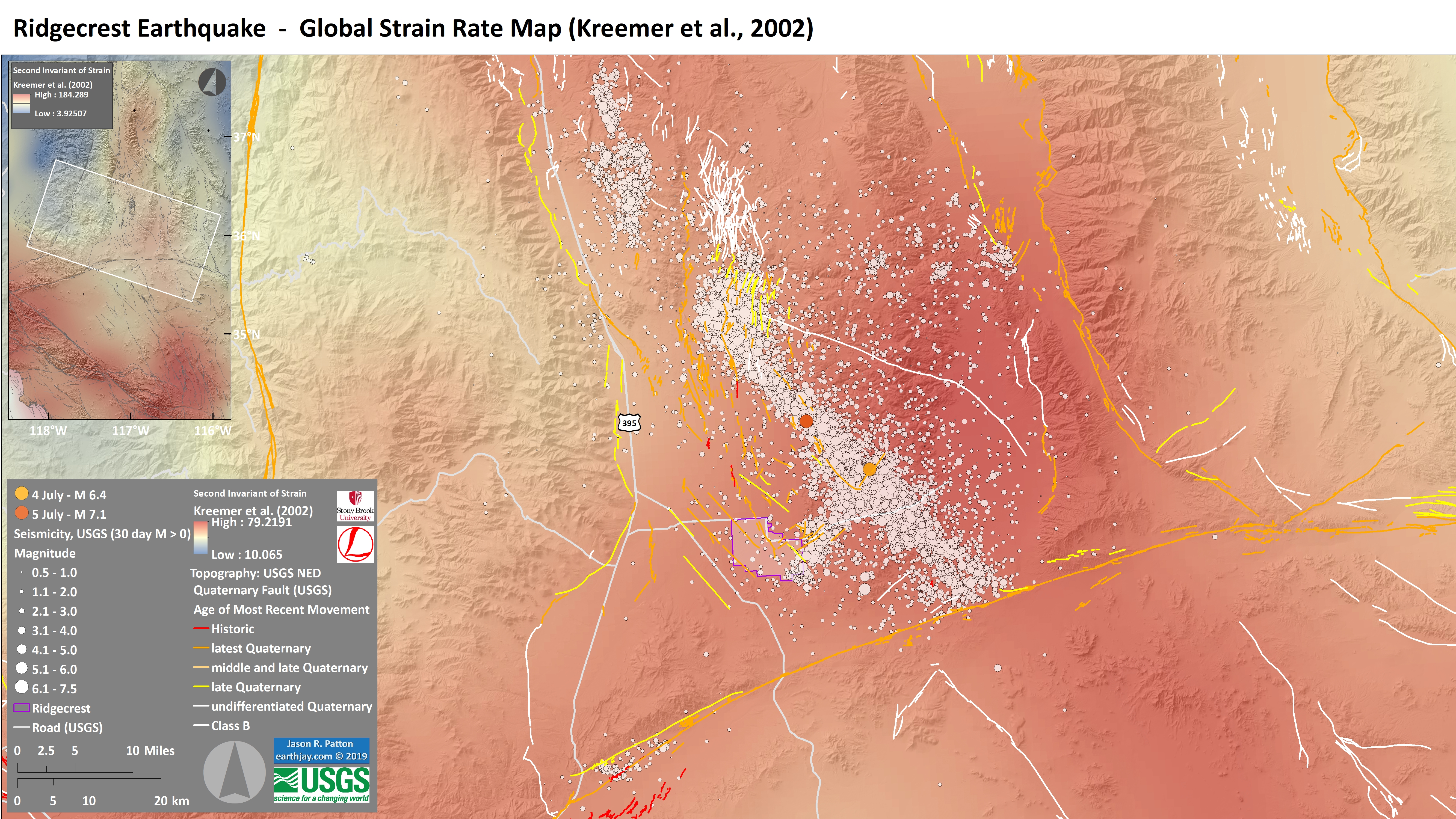
- 2019.07.20 M 6.4 / 7.1 Ridgecrest Update #3
- Strain is basically the change in shape or volume of a material through time. The Earth deforms with space and time in relation to geospatial variations in plate tectonic motions.
- Tectonic strain can be measured in a variety of methods. Most people are familiar with geodetic methods. Geodesy is the study of the motion of the Earth as measured at discrete locations (e.g. with GPS observations). One may use changes in position at GPS sites to measure how the Earth moves, so we can directly measure changes in shape this way.
- Geodetic data can be combined with geologic and seismicity data to evaluate tectonic strain at global, regional, and local scales.
- In 1998 the International Lithosphere Program started compiling a global dataset to support the construction of a Global Strain Rate Map (GSRM; Kreemer et al., 2000, 2002, 2003, 2014).
- The GSRM has been incorporated into the Global Earthquake Model of Seismic Hazard, v 2.1 presented online here.
- I present a map for the Ridgecrest Earthquake Sequence that uses an older version of the GSRM (v 1.2). The color ramp is based on the “second invariant” of strain. Warmer colors show regions of greater tectonic strain. Units are in 10
- There are some larger scale geology maps for this region, but they cost money (Dibblee Foundation/AAPG). Needless to say, I don’t have the $50 to buy them right now. They are geotiffs, so would overlay nicely.
- The map below shows seismicity for the past month overlain upon the 1962 California Division of Mines and Geology 1:250,000 scale geologic map (Jennings et al., 1962). I prepared this on 21 July 2019 after georeferencing the map from the CGS website..
There was a good sized earthquake in southern California today. The largest earthquake since the 1999 M 7.1 Hector Mine earthquake. (The 2003 San Simeon earthquake was larger, but much farther to the west, at about the same latitude.)
Today’s earthquake sequence has a mainshock (so far) with a magnitude M = 6.4.
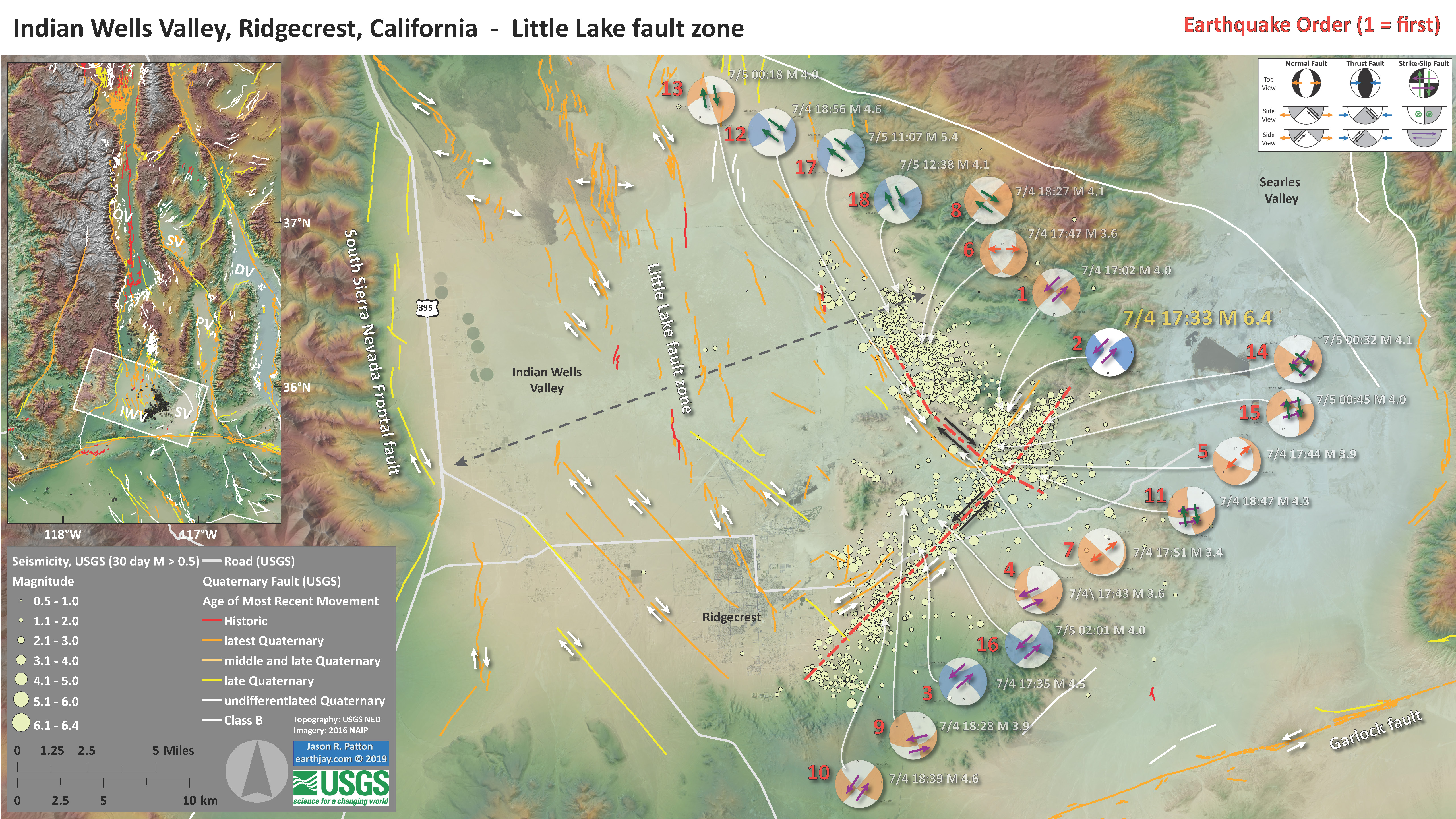
This region is at the intersection of several different fault systems. The Pacific-North America plate boundary, which most people associate with the San Andreas fault, includes the South Sierra Nevada fault zone and other right-lateral strike-slip faults that trend along the eastern side of the Sierra Nevada Mountains (including the Eastern California Shear Zone). There is also an interesting conjugate fault, the Garlock fault, which is a left-lateral strike-slip fault.
The sequence today appears to involve faults with both orientations. Looking at the aftershocks, it looks like the main shock is left-lateral (more aftershocks along the northeast trend).


There have been well over 1000 aftershocks with magnitudes M ≥ 0.5.
Last night there was the largest aftershock (so far) a magnitude M 5.4 earthquake.
It is clear that this sequence has involved at least 2 main faults. I interpret the mainshock (the M 6.4) to be on a northeast trending (striking) left-lateral strike-slip fault. This is largely because (1) the longer of the 2 aftershock trends is has this orientation and (2) the majority of field observations of surface rupture are along this orientation. The M 5.4 aftershock is located along the right-lateral northwest trending fault. The M 6.4 could be on the nw striking fault.
I prepared some interpretive posters for the M 7.1 earthquake shortly after it happened. The USGS earthquake pages are a source of great information as evidenced by how hard they are hit by web visitors following events as significant as the M 7.1. The website was unusable for periods of time. This demonstrates that the USGS is doing something right.
Last weekend, I spent Saturday preparing the same types of interpretive posters that I presented here, but as comparisons between the M 6.4 and M 7.1 temblors.


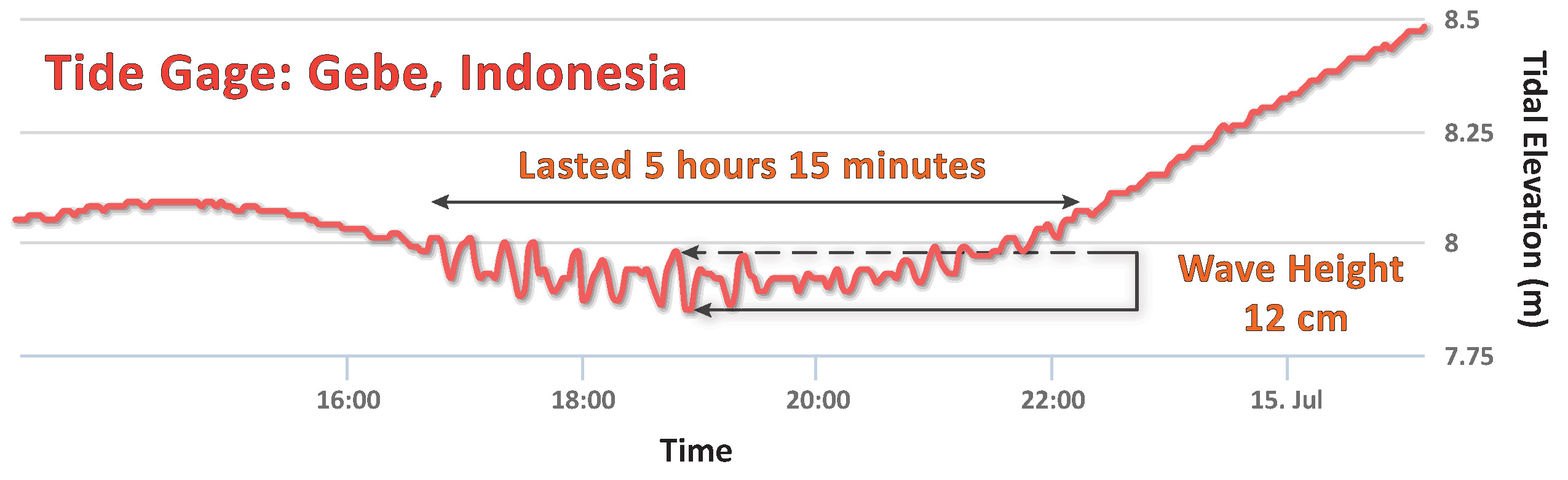
- 2019.07.14 M 7.3 Halmahera
- Here is the map with a month’s seismicity plotted.
There was an earthquake along Molucca Strait that I could not work on due to my field work. So I will briefly mention that quake here. There was also a recent earthquake to the south, in the Banda Sea (here is my earthquake report for that event). The June earthquake had the same magnitude as today’s shaker, M = 7.3. However, the earlier quake was too deep to cause a tsunami (unlike today’s temblor). Earthquakes along the Molucca Strait have generated tsunami with wave heights of over 9 meters (30 feet) according toe Harris and Major, 2016.
The Molucca Strait is a north-south oriented seaway formed by opposing subduction zone / thrust faults (convergent plate boundaries). See the “Geologic Fundamentals” section below for an explanation of different fault types. On the west of the Molucca Strait is a thrust fault that dips downwards to the west. On the east, there is a thrust fault that dips down to the east (beneath the island of Halmahera).
There is a major east-west trending (striking) strike-slip fault that comes into the region from the east, called the Sorong fault. There are multiple strands of this system. A splay of this Sorong fault splays northwards through the island of Halmahera. There may be additional details about how this splay relates to the Sorong fault, but I was unable to locate any references (or read the details) today. According to BMKG, the fault that is associated with this earthquake is the Sorong-Bacan fault.
Today’s M 7.3 Halmahera earthquake is a strike-slip earthquake (the plates move side-by-side, like the San Andreas or North Anatolia faults). Often people don’t think of tsunami when a strike-slip earthquake happens because there is often little vertical ground motion. Many people are otherwise familiar with thrust or subduction zone earthquakes, which can produce significant uplift and subsidence (vertical land motion), that can lead to significant tsunami.
Here is the tide gage record from a gage near today’s M 7.3 earthquake. The earthquake epicenter appears to be on land, so the tsunami is possibly smaller because of this. Indonesia operates a network of tide gages throughout the region here. The gage data below are from the island of Gebe, about 50 miles to the east of the M 7.3 epicenter.

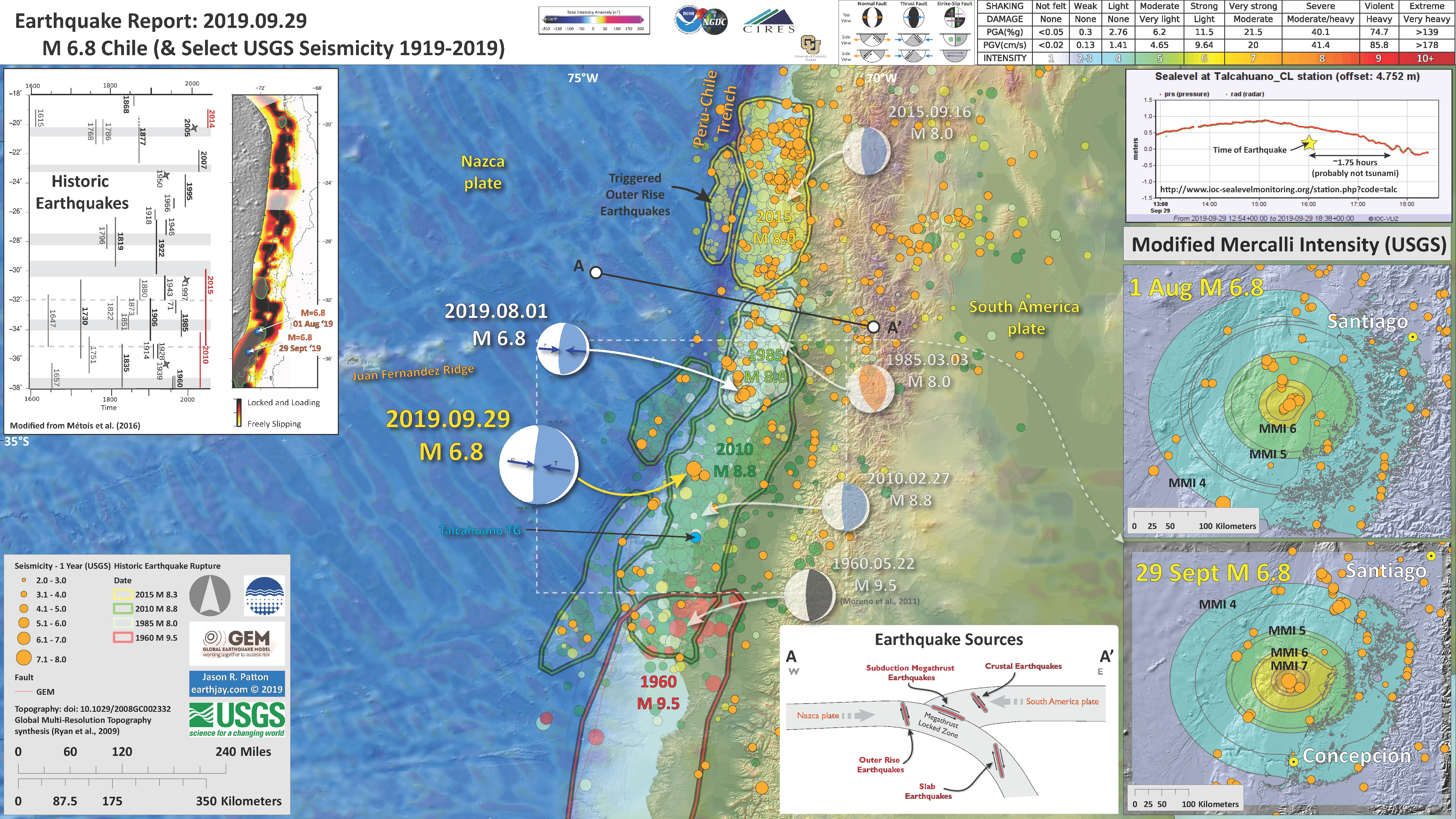
- 2019.08.01 M 6.8 Chile
- Here is the map with a century’s seismicity plotted, for earthquakes associated with the larger earthquakes from this region (colored relative to time scale, 1960, 1985, 2010, 2015, 2019).
- Here is a figure that shows a more detailed comparison between the modeled intensity and the reported intensity. Borth data use the same color scale, the Modified Mercalli Intensity Scale (MMI). More about this can be found here. The colors and contours on the map are results from the USGS modeled intensity. The DYFI data are plotted as colored dots (color = MMI, diameter = number of reports).
- In the lower right corner is a plot showing MMI intensity (vertical axis) relative to distance from the earthquake (horizontal axis). The models are represented by the green and orange lines. The DYFI data are plotted as light blue dots. The mean and median (different types of “average”) are plotted as orand and purple dots. Note how well the reports fit the green line (the model that represents how MMI works based on quakes in California). I plot Santiago relative to distance from the earthquake with a blue arrow (compare with the poster).
- Here is a poster that shows the significant earthquakes along this plate boundary. Note how there are earthquakes in the Nazca plate associated with the 2010 and 2015 megathrust subduction zone earthquakes. These are triggered earthquakes along the outer rise, not additional subduction zone earthquakes.
- In the lower right corner is a figure from Beck (1998) that shows the spatial extent of the known earthquakes. I added the extent of the 2015 and 2010 earthquakes as green arrows.
- In the upper right corner is an excellent figure from Horton (2018) that shows the plate tectonic setting for this area.
On 1 August 2019 there was an earthquake along the convergent plate boundary along the west coast of Chile (a subduction zone forming the Peru-Chile trench). This subduction zone megathrust fault produced the largest magnitude earthquake recorded on seismometers in 1960, the Valparaiso, Chile magnitude M9.5 earthquake that caused a trans-pacific tsunami causing damage and deaths all along the western hemispheric coastline.
This M 6.8 earthquake happened at the overlap of the southern end of the 1985 M8.0 and northern end of the 2010 M8.8 earthquakes.


- 2019.08.02 M 6.9 Indonesia
- Here is the map with a year’s (orange) and a century’s (gray) seismicity plotted.
- Below is the liquefaction susceptibility map. I discuss liquefaction more in my earthquake report on the 28 September 20018 Sulawesi, Indonesia earthquake, landslide, and tsunami here.
The tectonics are both simple and complicated in this part of the world. The islands of Sumatra and Java (and more) are rows of volcanoes (called an island arc) formed by the partial melt of mantle material associated with the subduction of the oceanic India-Australia plate beneath the Sunda plate (part of Eurasia).
So, the subduction zone is the main player on the scene. But the orientation (strike and changes in strike) of the subduction zone megathrust fault, in comparison to the relative motion between these plates, and in comparison to pre-existing structures in the India-Australia plate, leads to a number of additional faults.
The major fault system that accommodates the different relative plate motions is the Great Sumatra fault. The relative plate motion is oblique (not perpendicular to) the orientation of the subduction zone fault. Therefore, while the megathrust accommodates the fault perpendicular motion, the Sumatra accommodates the fault parallel motion (as a strike slip-fault). There are other strike slip faults too. These faults are called “forearc sliver faults.”
Some of the historic faults in the interpretive poster below are subduction zone earthquakes. The 2007 M 8.4 quake is a great example of this.
There are a couple good examples of “outer rise” earthquakes, temblors that occur in the downgoing plate, where there is flexure of the plate, causing the plate to bend and cause earthquakes along these bends. These are extensional earthquakes (the 2011 & 2013 quakes near Christmas Island).
The 2 Aug 2019 M 6.9 quake is interesting because it does not appear to be a megathrust quake, an outer rise quake, or a Sumatra fault quake. The M 6.9 is (1) too deep for those types of quakes and (2) has an orientation that is not consistent with those types of quakes. This quake is in the India-Australia plate and could be along a reactivated fracture zone. The inset maps shows several of these north-south trending fracture zones (e.g. the Investigator fracture zone).
Thus, I interpret this as a north-south oriented left-lateral strike-slip earthquake. It is pretty deep, and could also be related to some other processes going on within the slab or uppermost mantle. The slab depth at this location is 20 km, so the quake is possibly about 35 km beneath the top of the India Australia plate. Oceanic crust is, on average, 7km. So, this M 6.9 is probably within the mantle beneath the slab.
There is an analogous M 7.0 earthquake on 2009.09.02 to the east, just south of the label “Java” on the interpretive poster. This earthquake shows trench parallel compression (perpendicular to the compression from the subduction zone). This quake is almost 40 km deep, so is also probably beneath the slab, within the uppermost “lithospheric” mantle.
So, these 2019 M 6.9 and 2009 M 7.0 earthquakes are really cool.


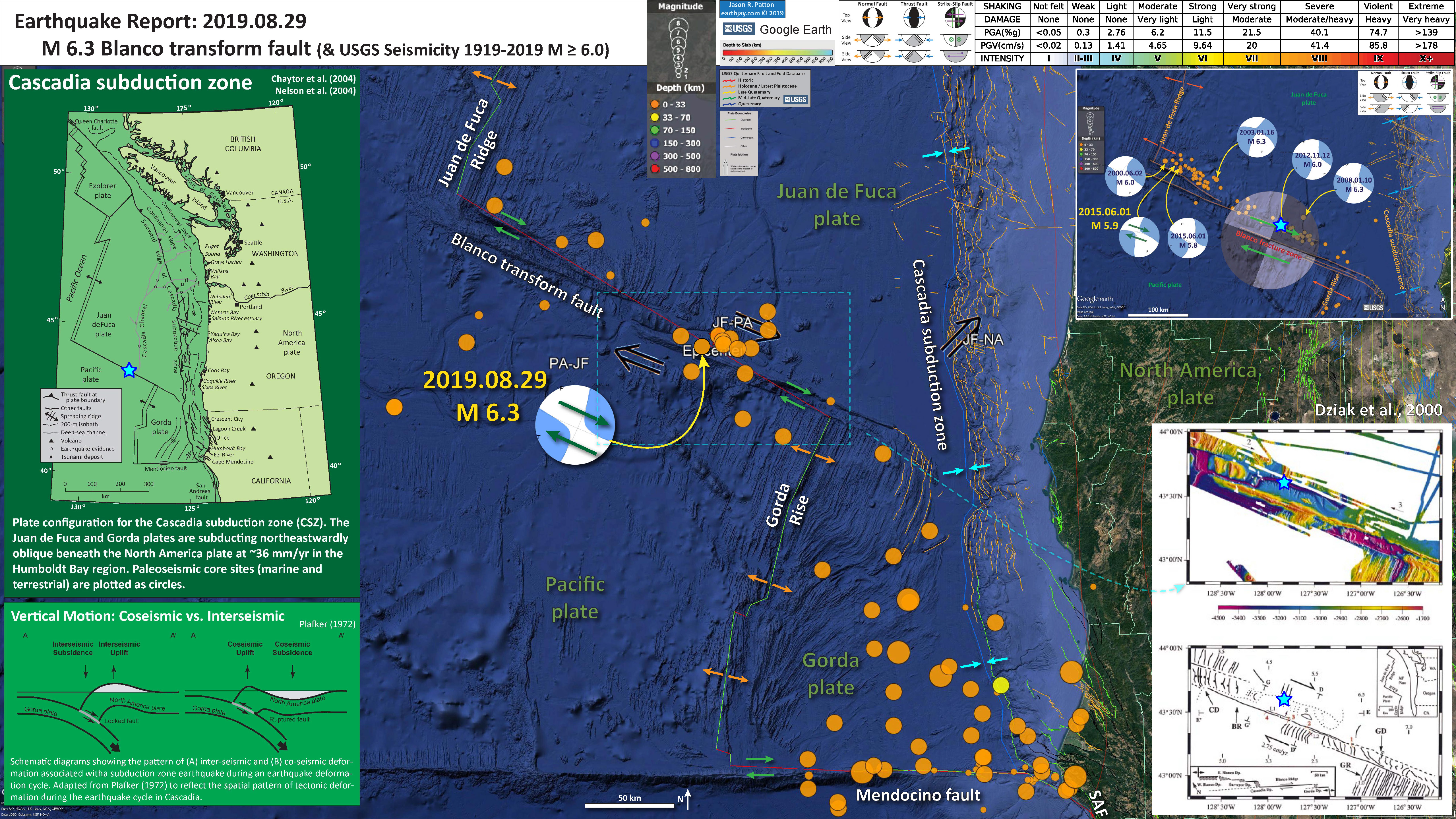
- 2019.08.29 M 6.3 Blanco transform fault
- Here is the map with a century’s seismicity plotted, for earthquakes of magnitude M ≥ 6.0.
The tectonics of the northeast Pacific is dominated by the Cascadia subduction zone, a convergent plate boundary, where the Explorer, Juan de Fuca, and Gorda oceanic plates dive eastward beneath the North America plate.
These oceanic plates are created (formed, though I love writing “created” in science writing) at oceanic spreading ridges/centers.
When oceanic spreading centers are offset laterally, a strike-slip fault forms called a transform fault. The Blanco transform fault is a right-lateral strike-slip fault (like the San Andreas fault). Thanks to Dr. Harold Tobin for pointing out why this is not a fracture zone.
This plate boundary fault system (BF) is quite active with ten magnitude M ≥ 6.0 earthquakes in the past 50 years (one every 5 years) and about 150 M ≥ 5 earthquakes in the same time range.
When there are quakes on the BF, people always wonder if the Cascadia megathrust is affected by this… “are we at greater risk because of those BF earthquakes?”
The main take away is that we are not at a greater risk because of these earthquakes. More on this below the interpretive poster.
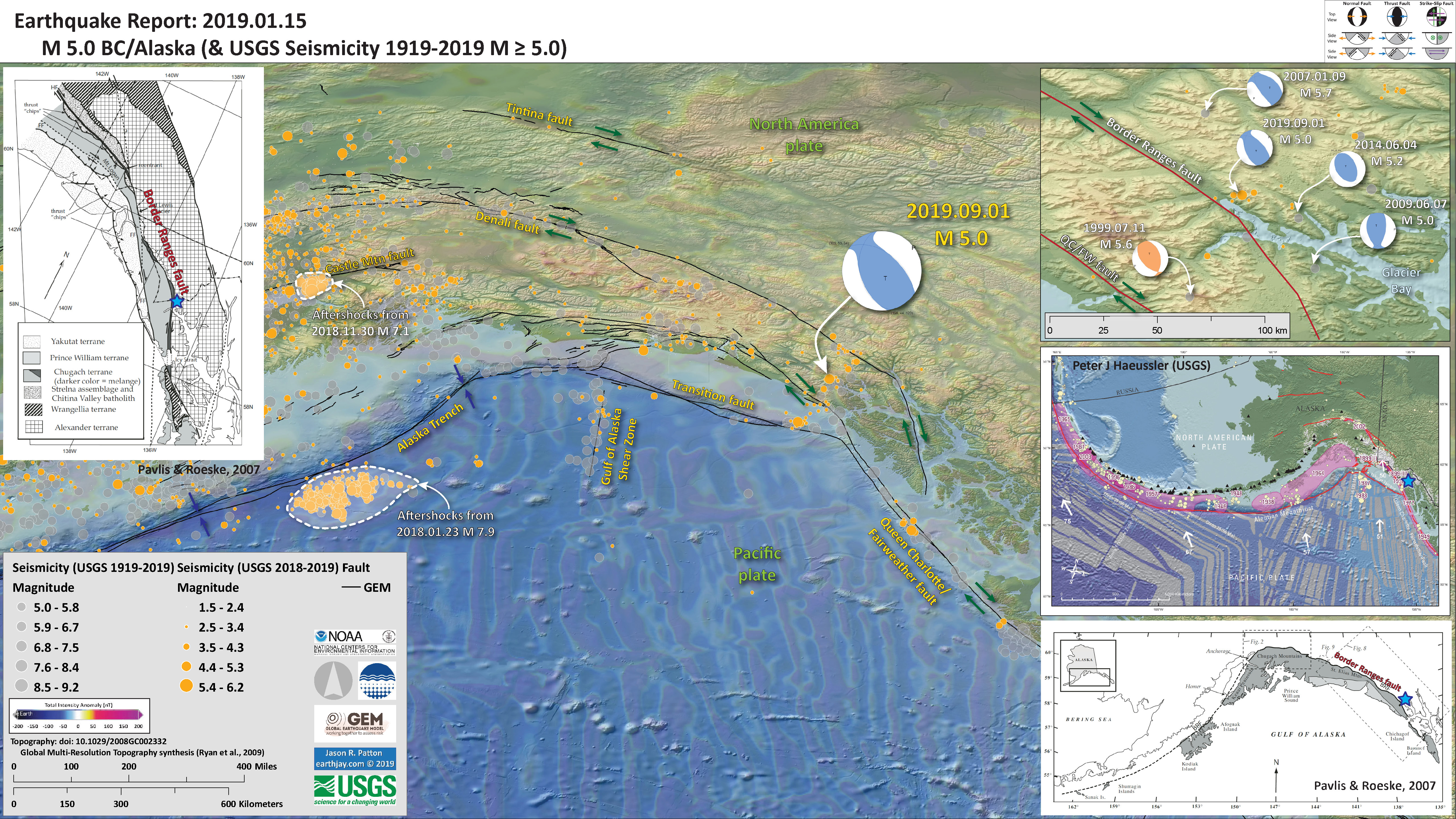
- 2019.09.01 M 5.0 BC/Alaska
https://earthquake.usgs.gov/earthquakes/eventpage/ak019b7lpbt4/executive
- 2019.09.24 M 6.0 Puerto Rico
https://earthquake.usgs.gov/earthquakes/eventpage/pr2019267000/executive

- 2019.09.25 M 6.5 Indonesia
https://earthquake.usgs.gov/earthquakes/eventpage/us70005lfd/executive
- 2019.09.29 M 6.8 Chile
https://earthquake.usgs.gov/earthquakes/eventpage/us70005nie/executive
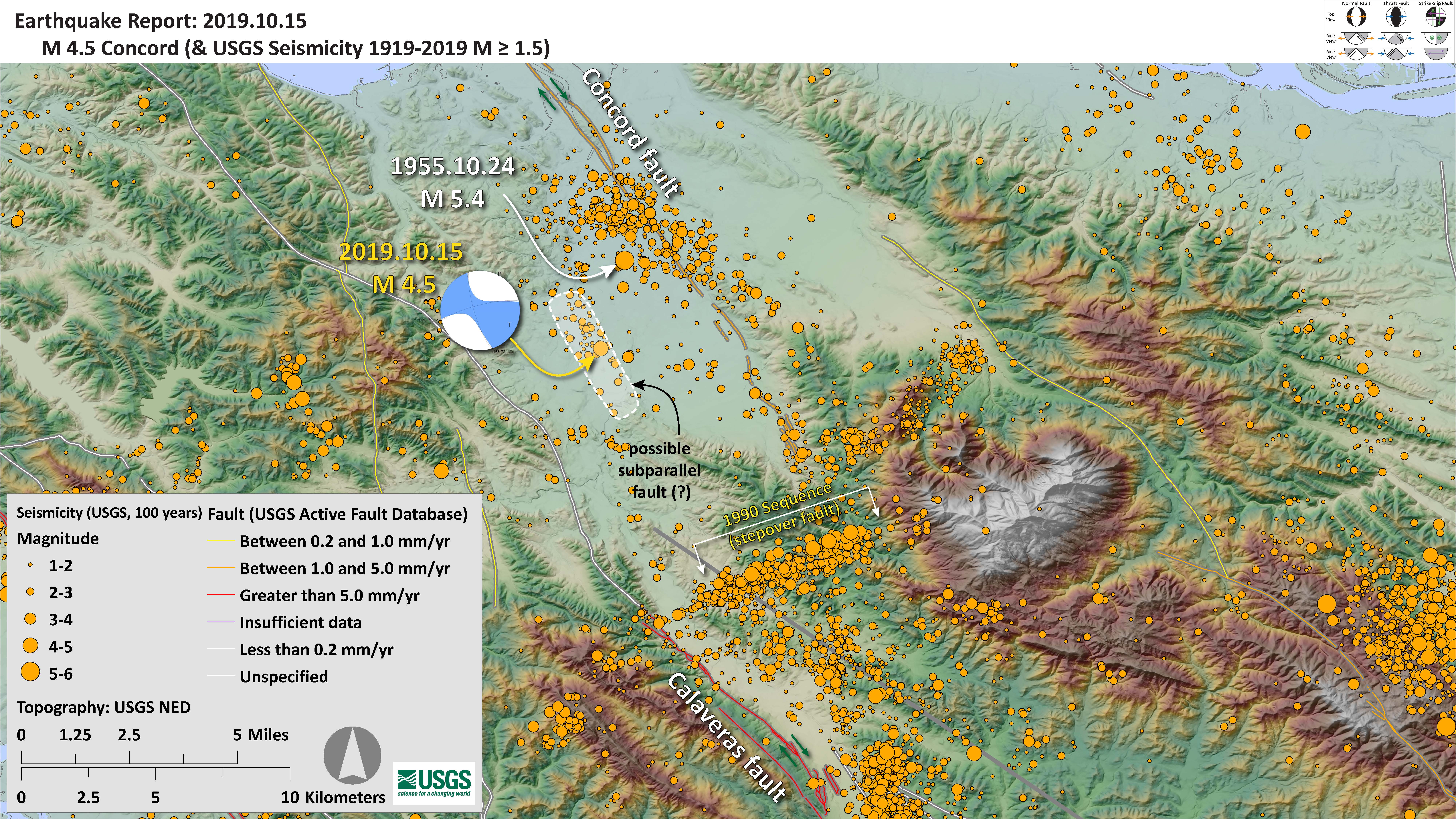
- 2019.10.15 M 4.5 Concord
https://earthquake.usgs.gov/earthquakes/eventpage/nc73291880/executive
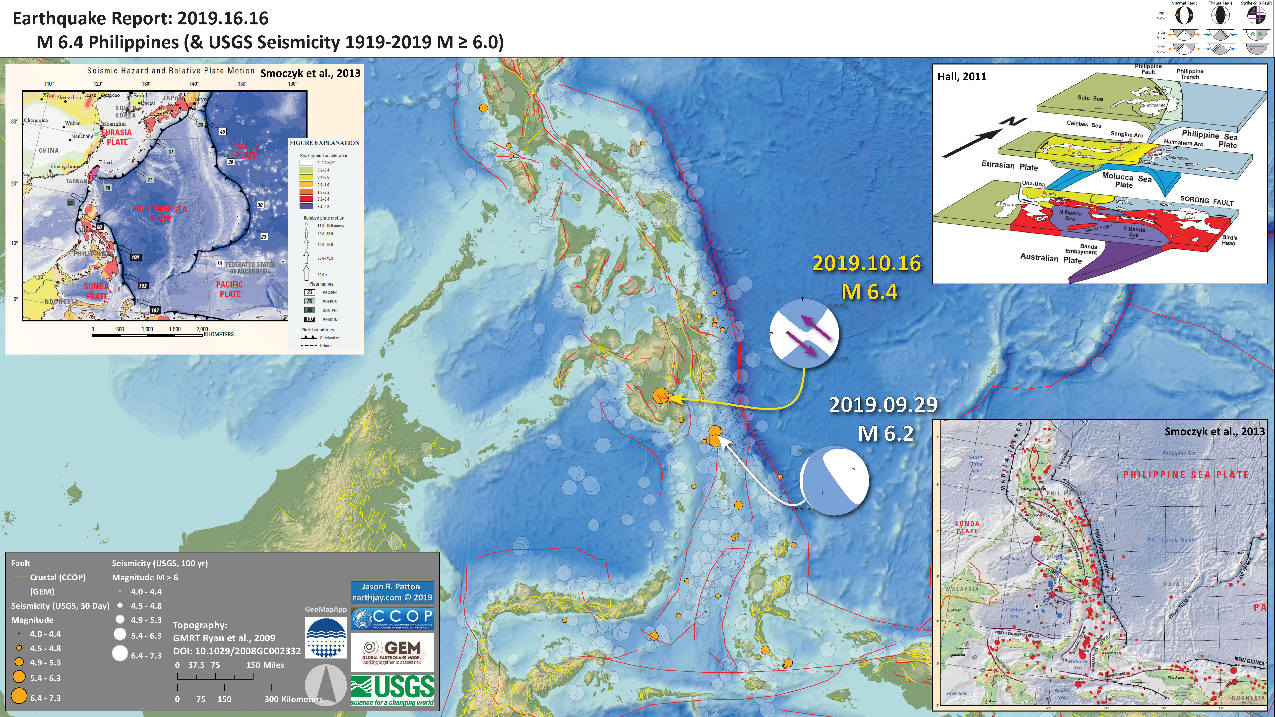
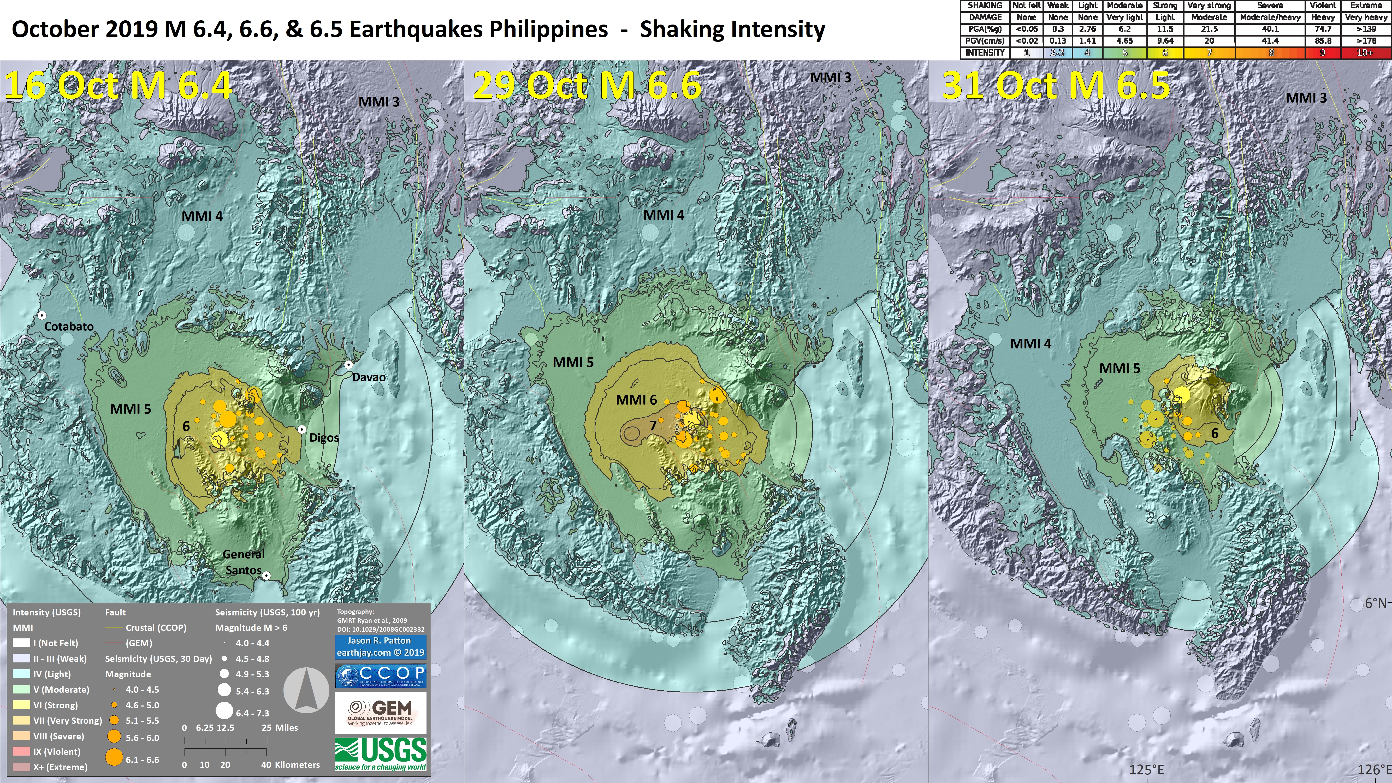
- 2019.10.15 M 6.4 Philippines
https://earthquake.usgs.gov/earthquakes/eventpage/us70005ulm/executive
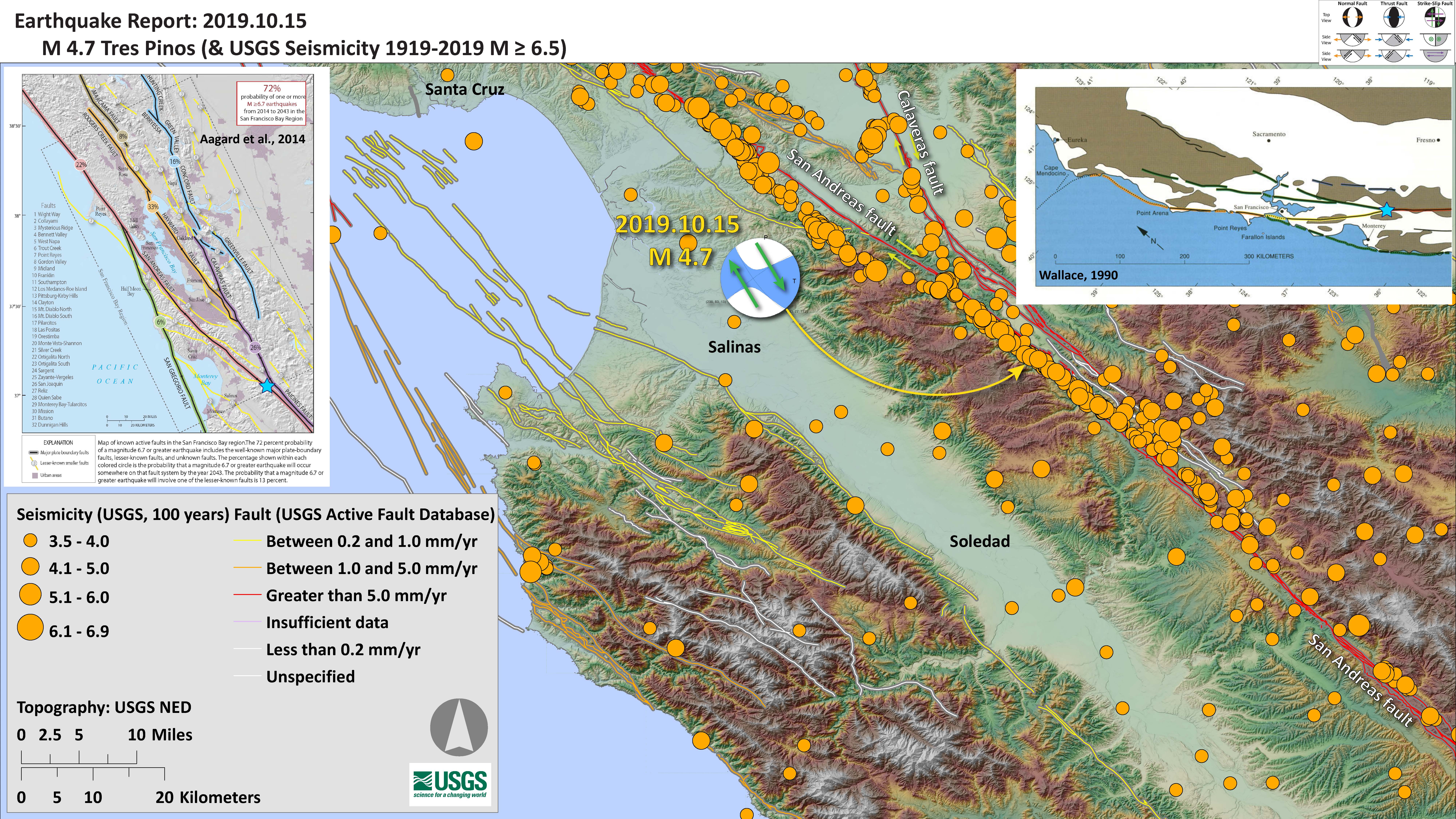
- 2019.10.15 M 4.7 Tres Pinos
https://earthquake.usgs.gov/earthquakes/eventpage/nc73292360/executive
- 2019.10.29 M 6.6 Philippines
https://earthquake.usgs.gov/earthquakes/eventpage/us6000645n/executive
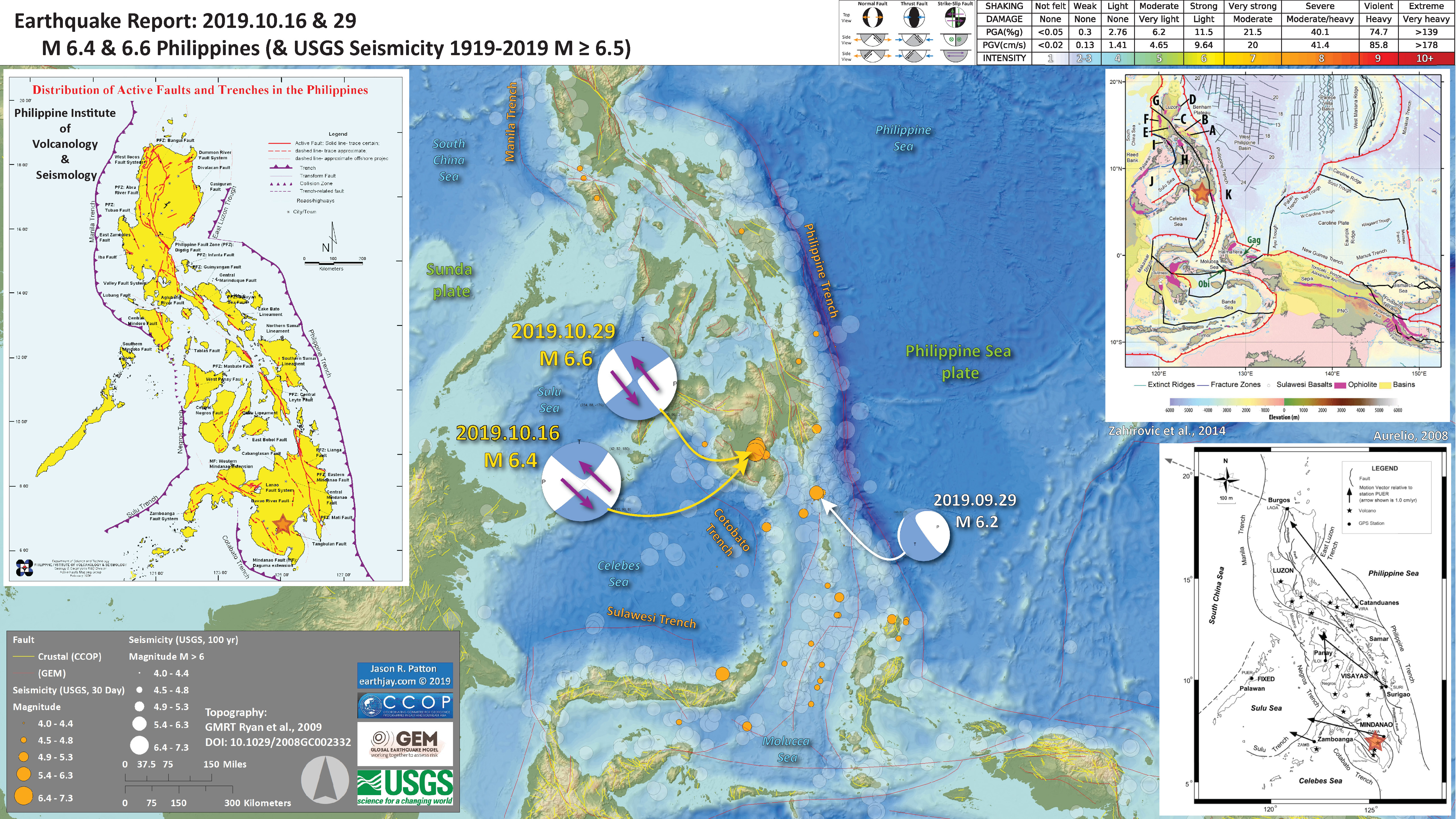
- 2019.10.31 M 6.5 Philippines
https://earthquake.usgs.gov/earthquakes/eventpage/us700061e9/executive
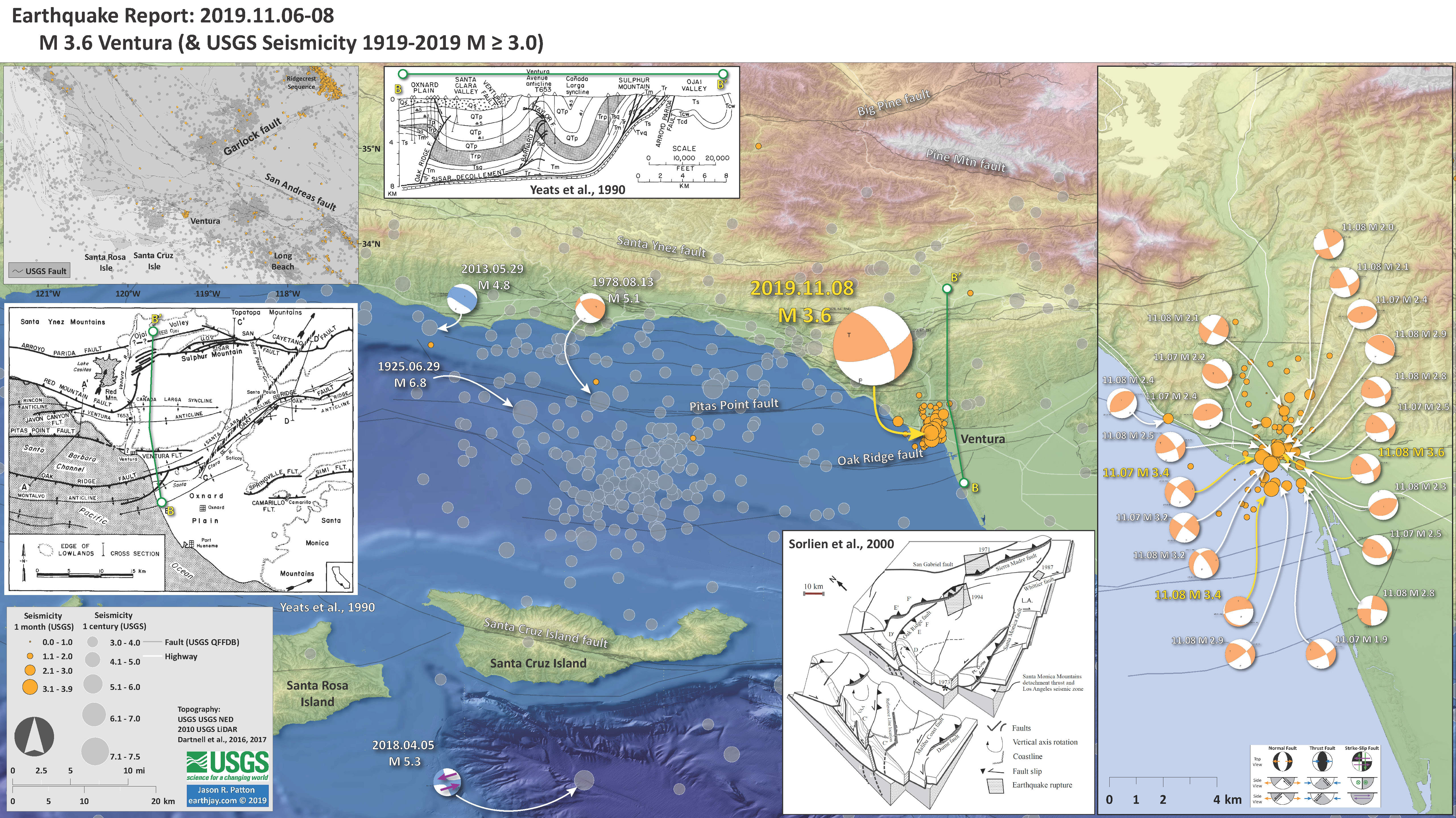
- 2019.11.08 M 3.6 Ventura
https://earthquake.usgs.gov/earthquakes/eventpage/ci38231786/executive
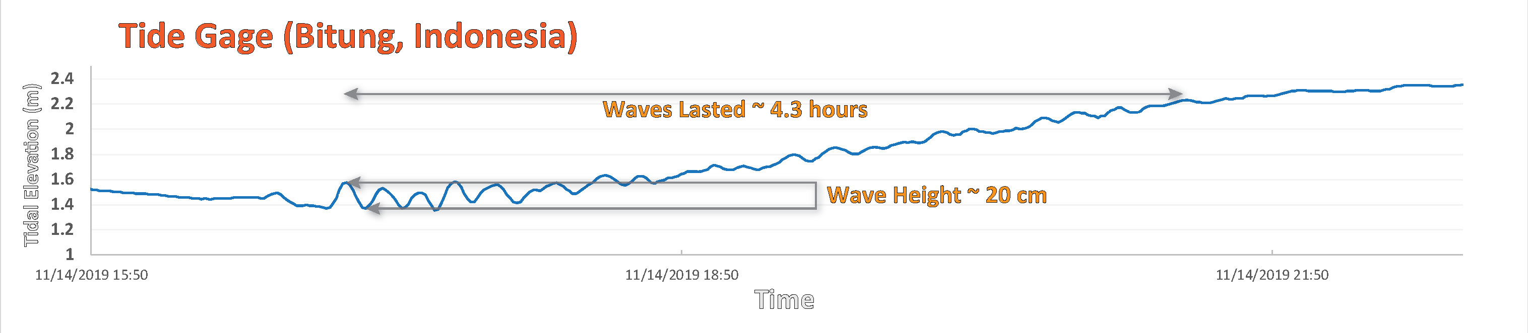
- 2019.11.14 M 7.1 Halmahera
There was a tsunamigenic earthquake in the Molucca Sea near Halmahera, Indonesia. Some of my earliest earthquake reports were from this region, but I have not had the opportunity to write anything up for earthquakes in this area for a few years.
The Halmahera Strait/Molucca Sea region is interesting as there is a pair of divergent subduction zones here. Basically, one dips to the east and one dips to the west, though it is a little more complicated.
McCaffrey et al. (1980) presented one of the first views of the subduction/thrust tectonics in this region. Since then, advances in marine geophysical methods have furthered our understanding and have generally re-enforced the early hypotheses rather well.
There was a minor tsunami recorded at a tide gage that was only 135 km (65 miles) from the epicenter. Here are those data plotted relative to time. The wave has a wave height of about 20 cm. The waves lasted several hours (it appears that maybe the waves resonated in the harbor).
Here is the interpretive poster.

Here is a map that shows shaking intensity using the MMI scale. The colors and black contours are from the USGS shaking intensity model. I also include some of the “Did You Feel It?” report observations (e.g. labeled “DYFI 4.9”).
In the upper left corner is a plot from the USGS that includes both modeled data (the orange and green lines) and DYFI data (the points and whisker plots). The legend informs us about the source of these different data.

- 2019.11.26 M 6.4 Albania
- There are 3 recognized faults in the area of this September/November sequence – the Vore, Shijak, and Lushnje faults.
- Given the data in the database, these faults may be capable of earthquakes with magnitudes of 5.5, 5.8, and 7.2 respectively.
- Most thrust faults in the region are southwest vergent (they dip down eastwards into the Earth). However, the Vore fault is northeast vergent.
- 1979 earthquake focal mechanisms along the Montenegro system are from Benetatos and Kiratzi (2006).
A couple days ago there was a deadly earthquake along the coast of Albania near the cities of Durrës and Mamurras. This M 6.4 earthquake caused many deaths and significant damage to buildings.
The west coast of Albania is a convergent plate boundary and there is a fold and thrust belt (thrust faults and folds formed due to the compression from plate convergence). Here, the Adria plate is diving beneath the Pelagonia (Eurasia) plate to form the Adriatic collision zone. The convergence here forms the Hellenides mountains. However, much of the tectonics in the region is currently extensional.
There was a sequence of earthquakes in September earlier this year. These are possibly either foreshocks to this November sequence, or they changed the stress in the surrounding crust to trigger the November sequence, or they are unrelated to the November sequence.
Below is my interpretive poster for this earthquake.

Below is a poster that shows possible fault sources.

Below is the liquefaction susceptibility and landslide probability map (Jessee et al., 2017; Zhu et al., 2017).
Please head over to that report for more information about the USGS Ground Failure products (landslides and liquefaction).

USGS Shaking Intensity
Here is a figure that shows a more detailed comparison between the modeled intensity and the reported intensity. Both data use the same color scale, the Modified Mercalli Intensity Scale (MMI). More about this can be found here. The colors and contours on the map are results from the USGS modeled intensity. The DYFI data are plotted as colored dots (color = MMI, diameter = number of reports)

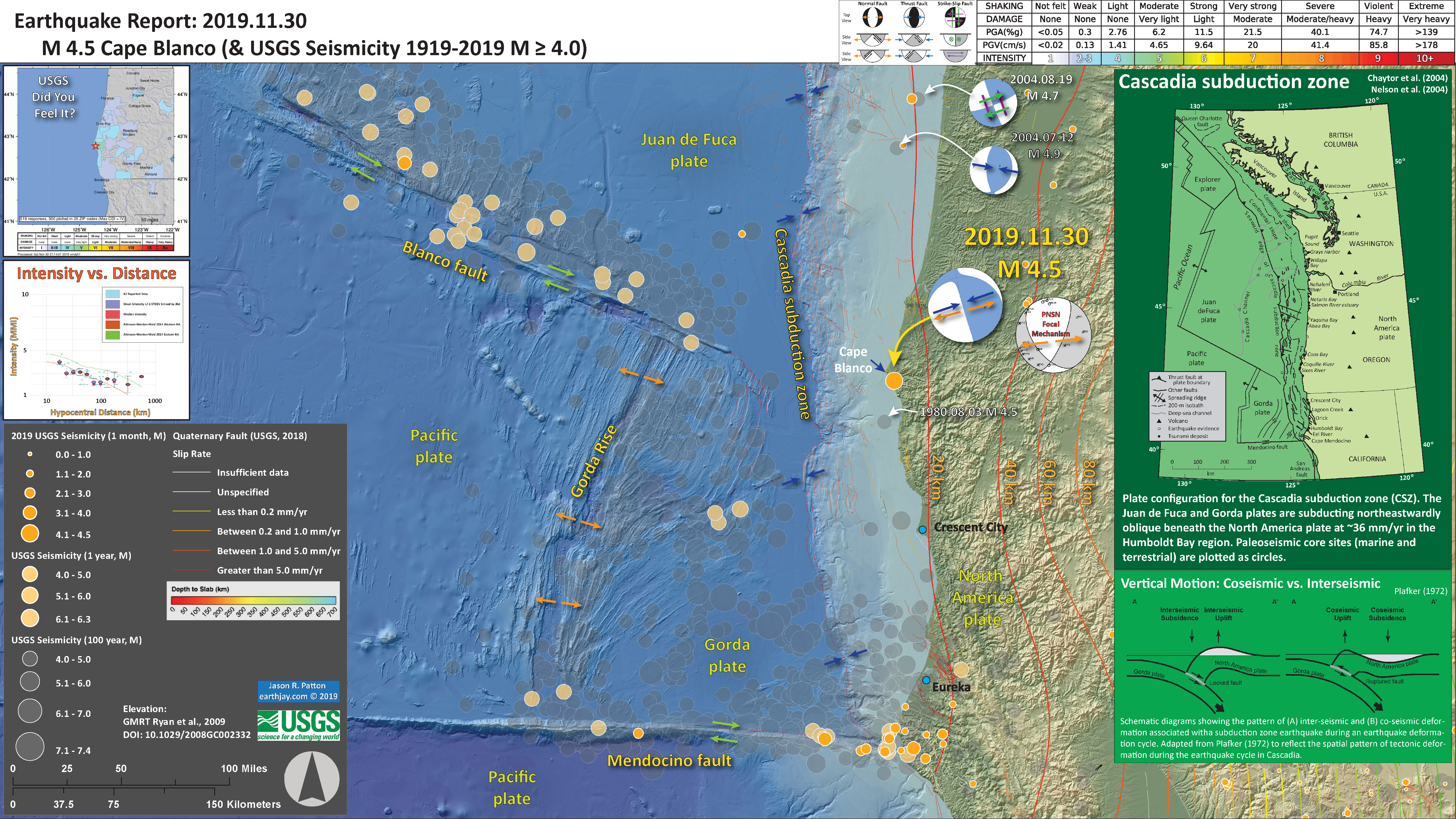
- 2019.11.30 M 4.5 Cape Blanco, Oregon
- This earthquake may be on the Cascadia megathrust subduction zone fault, or it may not.
https://earthquake.usgs.gov/earthquakes/eventpage/uw61562126/executive
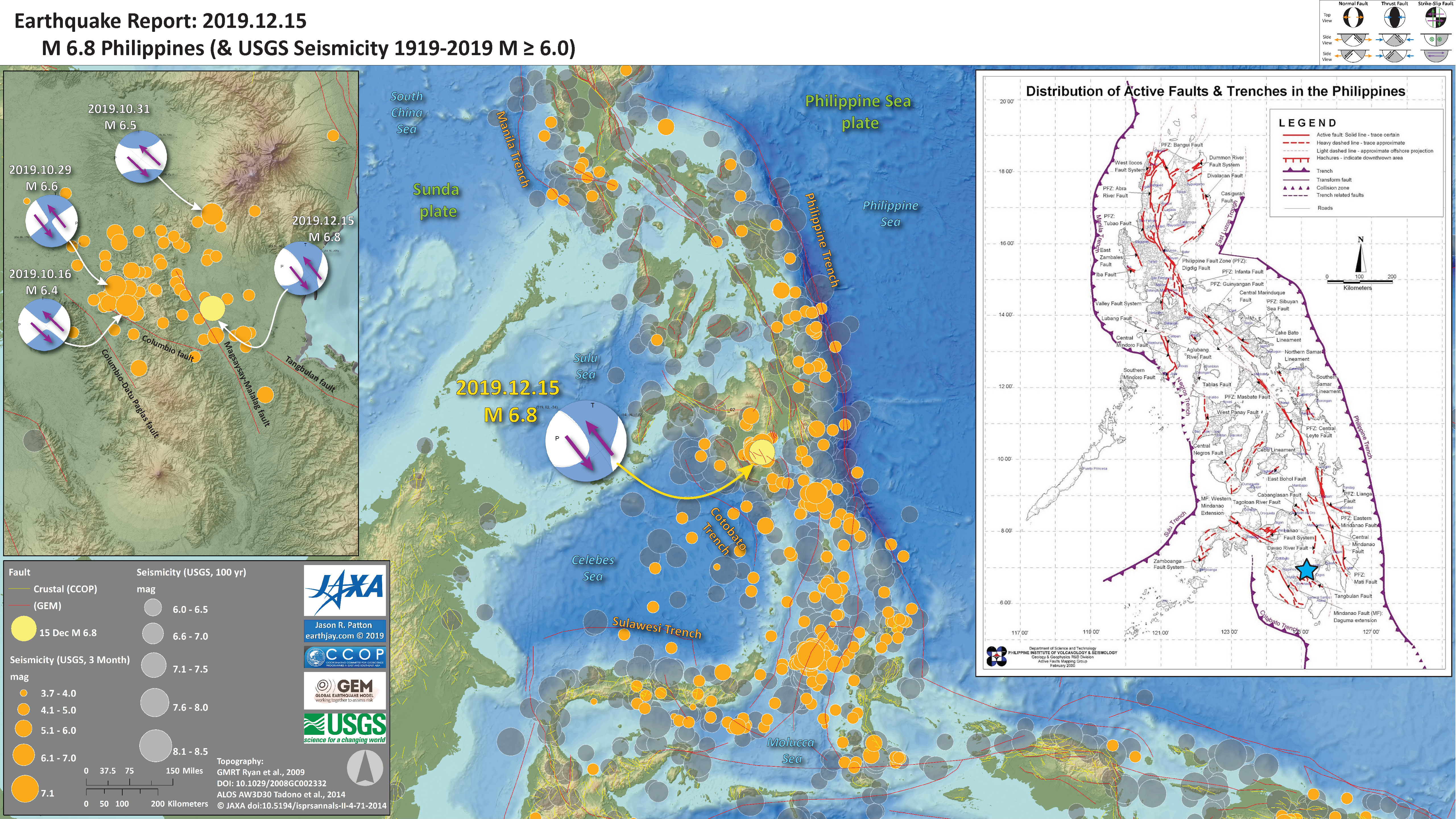
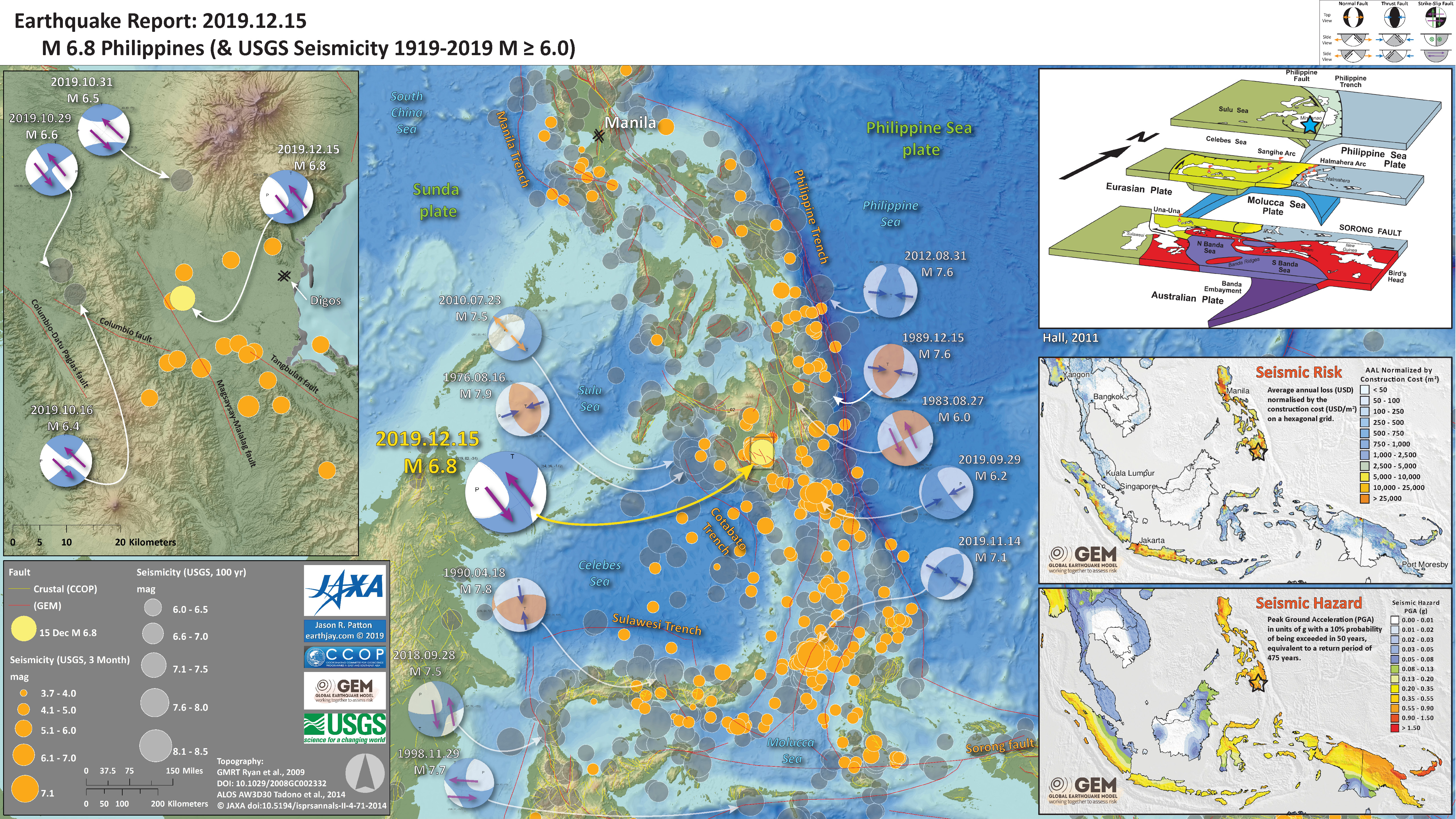
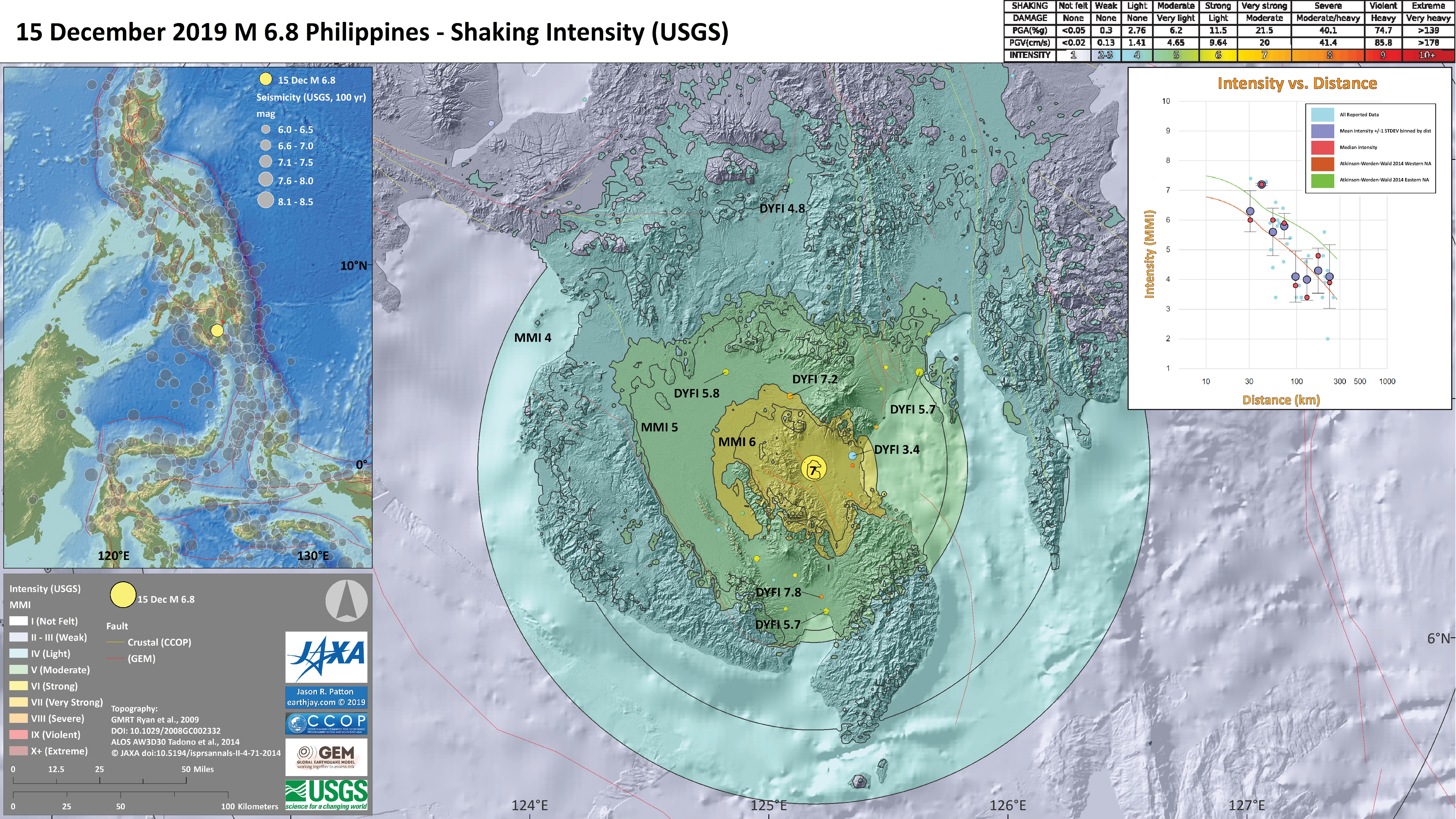
- 2019.12.15 M 6.8 Philippines
- Here is a version with more detailed presentation of the aftershocks. I also present the seismic hazard and seismic risk maps for the region from the Global Earthquake Model.
- This map shows a comparison of the USGS modeled intensity (in MMI scale) compared with USGS “Did You Feel It?” observations.
https://earthquake.usgs.gov/earthquakes/eventpage/us60006rp9/executive
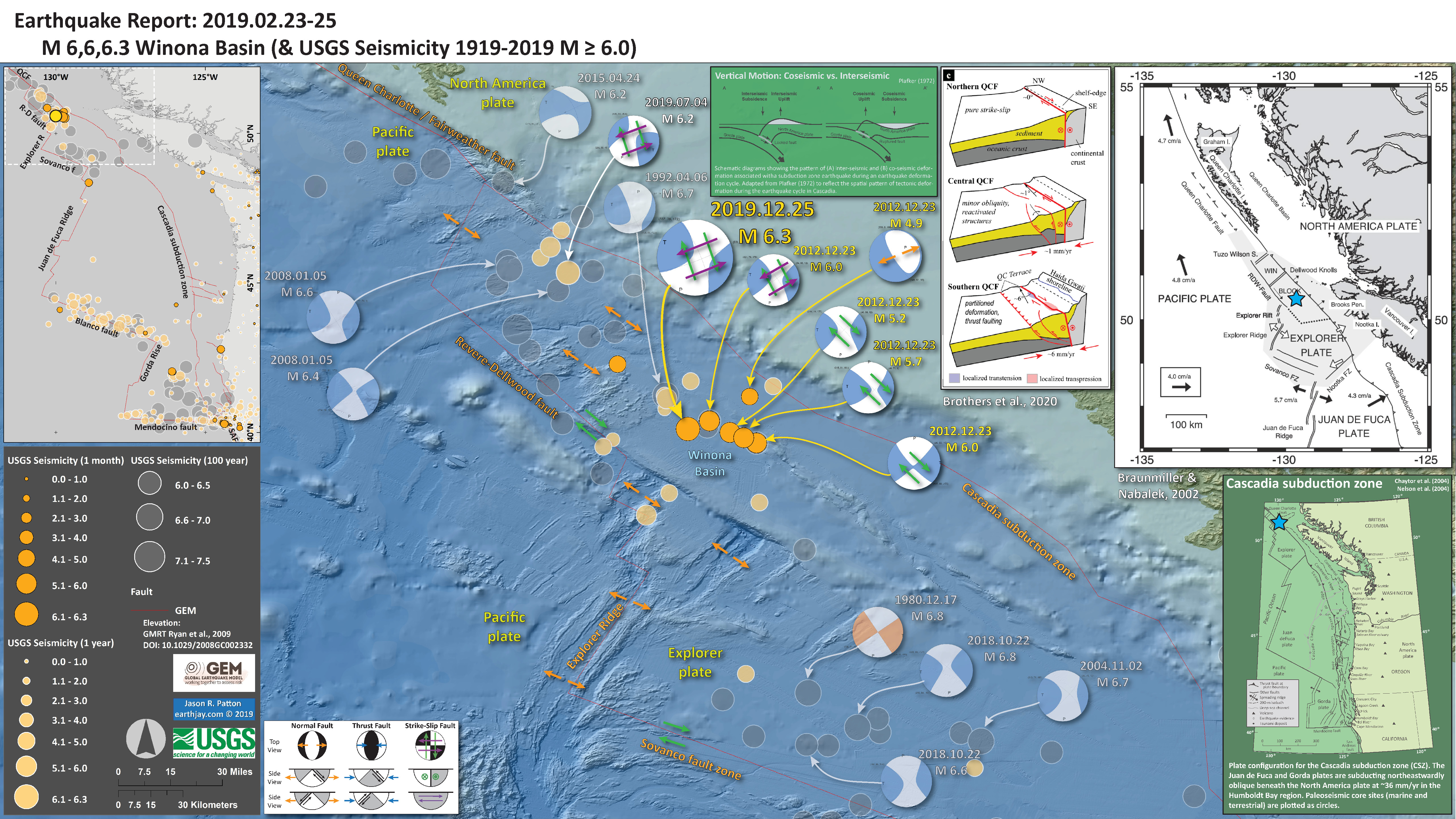
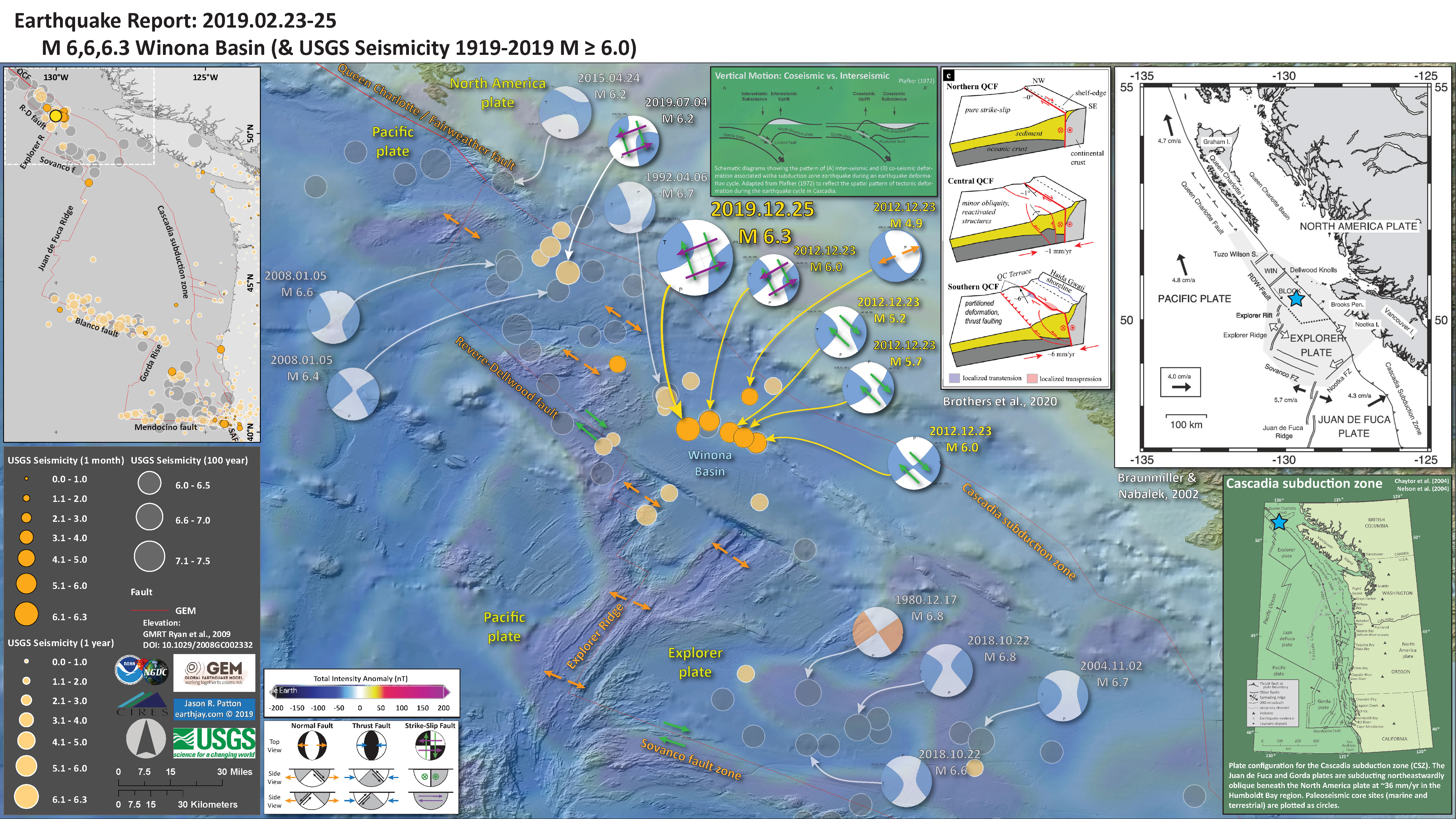
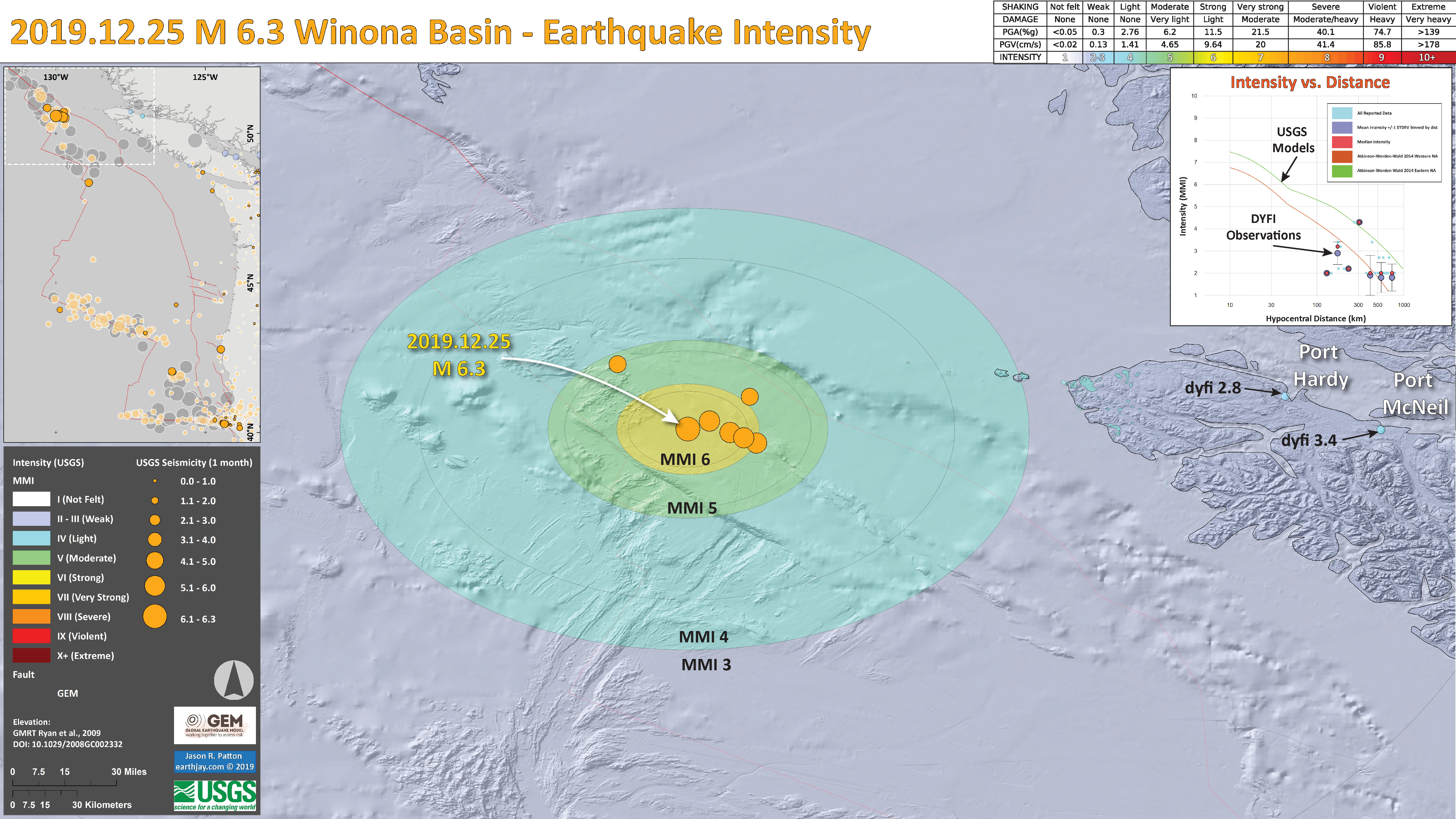
- 2019.12.23-25 M 6, 6, 6.3 Winona Basin, Canada
- The same map with magnetic anomaly data plotted. Note that these data show how the Explorer Ridge splays into two spreading ridges on the north end (the red along the ridge is a positive anomaly, which means that it has the same polarity as the modern North-South pole system).
- This map shows a comparison of the USGS modeled intensity (in MMI scale) compared with USGS “Did You Feel It?” observations.
https://earthquake.usgs.gov/earthquakes/eventpage/us70006qt7/executive
- 2019.12.29 M 5.0 Puerto Rico
https://earthquake.usgs.gov/earthquakes/eventpage/pr2019363002/executive

Return to the Earthquake Reports page.
#EarthquakeReport 2019 Significant Seismic Summary#Earthquake #Gempa #Lindol #Terremoto #Temblor #Tsunami #Landslide #Liquefaction
Annual Review of reports and posters herehttps://t.co/9nYtMuAePo pic.twitter.com/ULTHiPw4Wk
— Jason "Jay" R. Patton (@patton_cascadia) December 31, 2019
#EarthquakeReport 2019 Annual Seismic Summary#Earthquakes with magnitudes M ≥ 6.5
earthquake posters here https://t.co/9nYtMuAePo pic.twitter.com/7HDJQ7Mm5z
— Jason "Jay" R. Patton (@patton_cascadia) January 8, 2020