
Well, yesterday while I was installing the final window in a reconstruction project, there was an earthquake along the Aleutian Island Arc (a subduction zone) in the region of the Andreanof Islands. Here is the USGS website for the M 6.6 (now M 6.5) earthquake. This earthquake is close to the depth of the megathrust fault, but maybe not close enough. So, this may be on the subduction zone, but may also be on an upper plate fault (I interpret this due to the compressive earthquake fault mechanism). The earthquake has a hypocentral depth of 20 km (now 33.9 km, so much more likely on the megathrust) and the slab model (see Hayes et al., 2013 below and in the poster) is at 40 km at this location. There is uncertainty in both the slab model and the hypocentral depth.
The Andreanof Islands is one of the most active parts of the Aleutian Arc. There have been many historic earthquakes here, some of which have been tsunamigenic (in fact, the email that notified me of this earthquake was from the ITIC Tsunami Bulletin Board).
Possibly the most significant earthquake was the 1957 Andreanof Islands M 8.6 Great (M ≥ 8.0) earthquake, though the 1986 M 8.0 Great earthquake is also quite significant. As was the 1996 M 7.9 and 2003 M 7.8 earthquakes. Lest we forget smaller earthquakes, like the 2007 M 7.2. So many earthquakes, so little time.
I include some earthquakes along this plate boundary system that are also interesting as they reveal how the plate boundary changes along strike, and how the margins of the plate boundary (e.g. the western and eastern termini) behave.
The M 6.6 (now M 6.5) earthquake is the result of north-northwest compression from the subduction of the Pacific plate underneath the North America plate to the north.
The majority of the Aleutian Islands are volcanic arc islands formed as a result of the subduction of the Pacific plate beneath the North America plate. As the oceanic crust subducts, the water in the rock tends is released into the overlying mantle, leading to magma formation. This magma is less dense and rises to form volcanoes that comprise this magmatic arc.
This and other earthquakes have occurred in the region of the subduction zone west of where the Adak fracture zone is aligned. Further to the east is the Amlia fracture zone. The Amlia fracture zone is a left lateral strike slip oriented fracture zone, which displaces crust of unequal age, beneath the megathrust. The difference in age results in a variety of factors that may contribute to differences in fault stress across the fracture zone (buoyancy, thermal properties, etc). For example, older crust is colder and denser, so it sinks lower into the mantle and exerts a different tectonic force upon the overriding plate.
To the west, there is another subduction zone along the Kuril and Kamchatka volcanic arcs. These subduction zones form deep sea trenches (the deepest parts of the ocean are in subduction zone trenches). Between these 2 subduction zones is another linear trough, but this does not denote the location of a subduction zone. The plate boundary between the Kamchatka and Aleutian trenches is the Bering Kresla shear zone (BKSZ). Below I present some earthquake reports that help explain the western terminus of the Aleutian subduction zone.
This earthquake sequence is unrelated to the earthquakes in northern Alaska earlier this week. Here is my report for that sequence.
There was also a sequence (that is still experiencing aftershocks) in the Gulf of Alaska. Here is my main report (there were updates) for this Gulf of Alaska earthquake.
Below is my interpretive poster for this earthquake
I plot the seismicity from the past month, with color representing depth and diameter representing magnitude (see legend). I include earthquake epicenters from 1918-2018 with magnitudes M ≥ 3.0 in one version.
I plot the USGS fault plane solutions (moment tensors in blue and focal mechanisms in orange), in addition to some relevant historic earthquakes.
Mechanisms for historic earthquakes that come from publications other than the USGS fault plane solutions include the 1957 M 8.7 (Brown et al., 2013), the 1965 M 8.7 (Stauyder, 1968), and the 1965 M 7.6 earthquakes (Abe, 1972).
- I placed a moment tensor / focal mechanism legend on the poster. There is more material from the USGS web sites about moment tensors and focal mechanisms (the beach ball symbols). Both moment tensors and focal mechanisms are solutions to seismologic data that reveal two possible interpretations for fault orientation and sense of motion. One must use other information, like the regional tectonics, to interpret which of the two possibilities is more likely.
- I also include the shaking intensity contours on the map. These use the Modified Mercalli Intensity Scale (MMI; see the legend on the map). This is based upon a computer model estimate of ground motions, different from the “Did You Feel It?” estimate of ground motions that is actually based on real observations. The MMI is a qualitative measure of shaking intensity. More on the MMI scale can be found here and here. This is based upon a computer model estimate of ground motions, different from the “Did You Feel It?” estimate of ground motions that is actually based on real observations.
- I include the slab contours plotted (Hayes et al., 2012), which are contours that represent the depth to the subduction zone fault. These are mostly based upon seismicity. The depths of the earthquakes have considerable error and do not all occur along the subduction zone faults, so these slab contours are simply the best estimate for the location of the fault.
- In the map below, I include a transparent overlay of the magnetic anomaly data from EMAG2 (Meyer et al., 2017). As oceanic crust is formed, it inherits the magnetic field at the time. At different points through time, the magnetic polarity (north vs. south) flips, the north pole becomes the south pole. These changes in polarity can be seen when measuring the magnetic field above oceanic plates. This is one of the fundamental evidences for plate spreading at oceanic spreading ridges (like the Gorda rise).
- Regions with magnetic fields aligned like today’s magnetic polarity are colored red in the EMAG2 data, while reversed polarity regions are colored blue. Regions of intermediate magnetic field are colored light purple.
- We can see the roughly east-west trends of these red and blue stripes. These lines are parallel to the ocean spreading ridges from where they were formed. The stripes disappear at the subduction zone because the oceanic crust with these anomalies is diving deep beneath the Sunda plate (part of Eurasia), so the magnetic anomalies from the overlying Sunda plate mask the evidence for the Australia plate.
Magnetic Anomalies
- In the upper center is a map from IRIS that shows seismicity plotted relative to depth using color. One may observe that the earthquakes get deeper to the north, relative to the subduction zone fault (labeled Aleutain Trench in the posters below). I place a yellow star in the general location of this earthquake sequence (same for other figures here).
- In the center right is a companion figure from IRIS that shows a low angle oblique view of this Pacific – North America plate boundary. Note how the downgoing Pacific plate subducts beneath the North America plate as a megathrust fault.
- In the lower left corner is a figure from Torsvik et al. (2017) which shows the age progression for the seamounts along the Emperor and Hawai’i seamount chains. This age progression is a key evidence for plate tectonic theory and a foundation for our knowledge of plate motion rates globally.
- In the lower right corner is a figure from Sykes et al. (1980) that includes a map and a space-time diagram (shows spatial extent and timing for historic earthquakes along various fault systems.
- In the upper right corner is a figure that shows the historic earthquake ruptures along the Aleutian Megathrust (Peter Haeussler, USGS).
I include some inset figures.
- Here is the map with a month’s seismicity plotted.
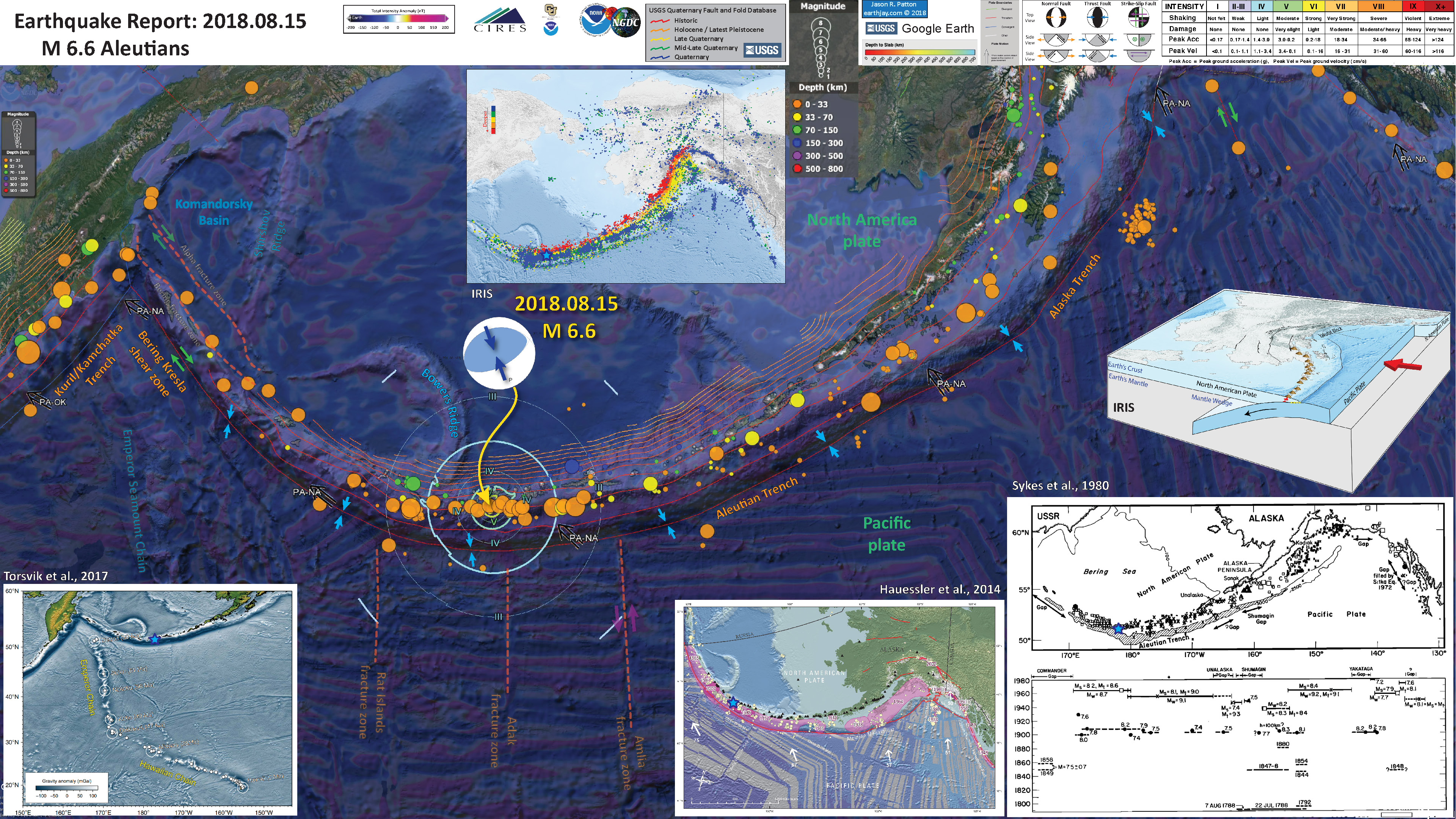
- Here is the map with a centuries seismicity plotted for earthquakes M ≥ 6.6.

Other Report Pages
Some Background about the North America – Pacific plate boundary
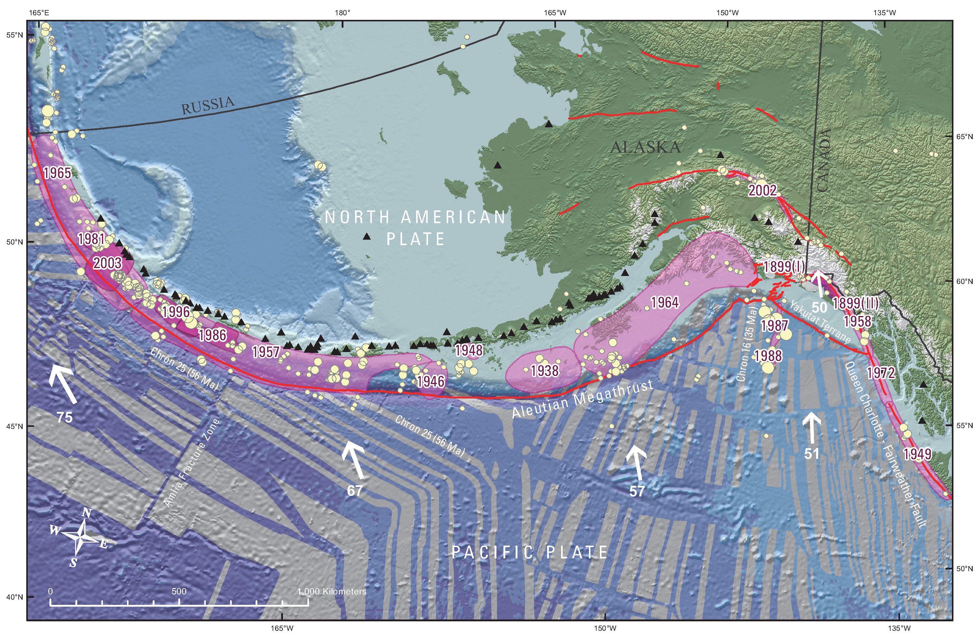
- Here is a map that shows historic earthquake slip regions as pink polygons (Peter Haeussler, USGS). Dr. Haeussler also plotted the magnetic anomalies (grey regions), the arc volcanoes (black diamonds), and the plate motion vectors (mm/yr, NAP vs PP).
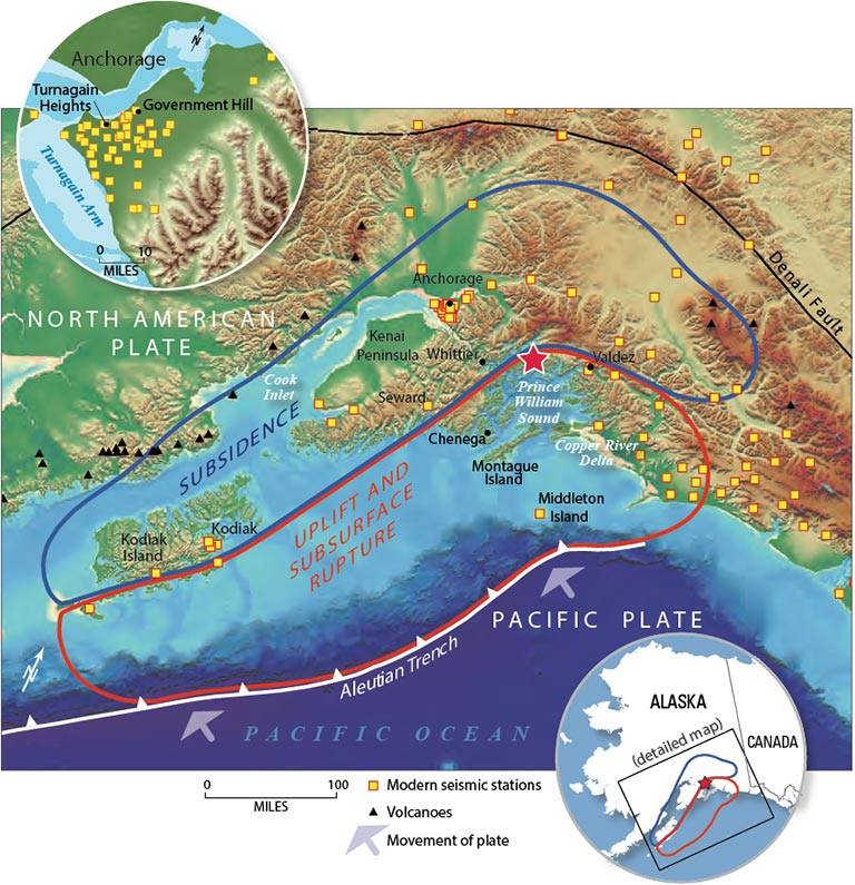
- Speaking of the 1964 earthquake, here is a map that shows the regions of coseismic uplift and subsidence observed following that earthquake. The 27 March, 1964 M 9.2 earthquake is the second largest earthquake ever recorded on modern seismometers. This figure can be compared to the cross section below.
- Here is the Plafker (1972)cross-section graphic on its own.
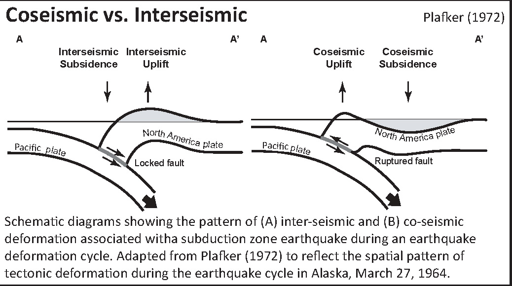
- Here is a figure recently published in the 5th International Conference of IGCP 588 by the Division of Geological and Geophysical Surveys, Dept. of Natural Resources, State of Alaska (State of Alaska, 2015). This is derived from a figure published originally by Plafker (1969). There is a cross section included that shows how the slip was distributed along upper plate faults (e.g. the Patton Bay and Middleton Island faults).
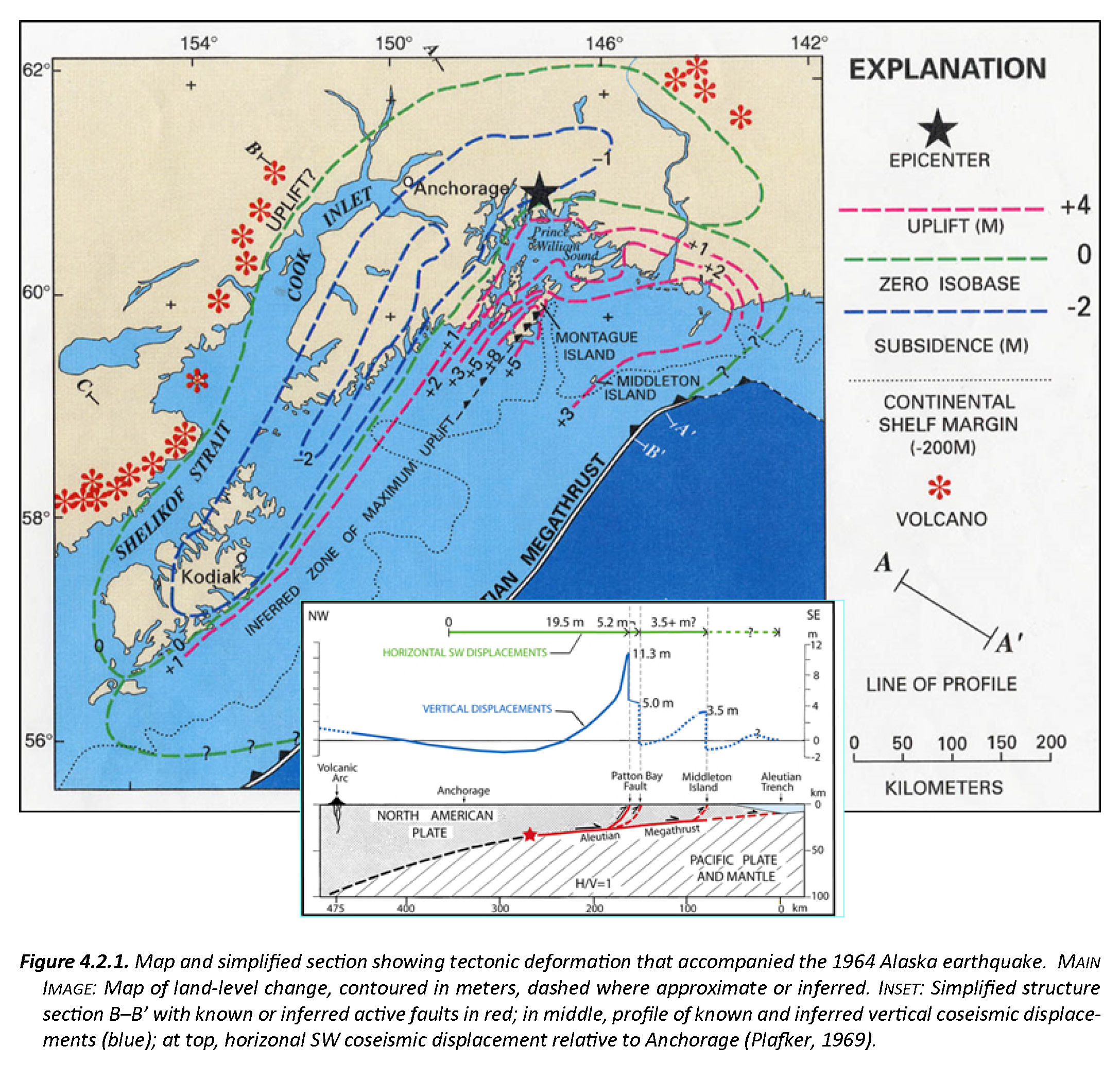
- This figure shows a summary of the measured horizontal and vertical displacements from the Good Friday Earthquake. I include a figure caption from here below as a blockquote.
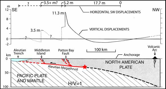
Profile and section of coseismic deformation associated with the 1964 Alaska earthquake across the Aleutian arc (oriented NW-SE through Middleton and Montague Islands). Profile of horizontal and vertical components of coseismic slip (above) and inferred slip partitioning between the megathrust and intraplate faults (below). From Plafker (1965, 1967; 1972)
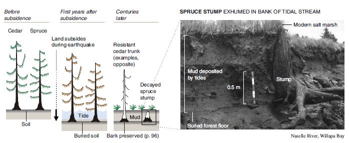
- Here is a graphic showing the sediment-stratigraphic evidence of earthquakes in Cascadia, but the analogy works for Alaska also. Atwater et al., 2005. There are 3 panels on the left, showing times of (1) prior to earthquake, (2) several years following the earthquake, and (3) centuries after the earthquake. Before the earthquake, the ground is sufficiently above sea level that trees can grow without fear of being inundated with salt water. During the earthquake, the ground subsides (lowers) so that the area is now inundated during high tides. The salt water kills the trees and other plants. Tidal sediment (like mud) starts to be deposited above the pre-earthquake ground surface. This sediment has organisms within it that reflect the tidal environment. Eventually, the sediment builds up and the crust deforms interseismically until the ground surface is again above sea level. Now plants that can survive in this environment start growing again. There are stumps and tree snags that were rooted in the pre-earthquake soil that can be used to estimate the age of the earthquake using radiocarbon age determinations. The tree snags form “ghost forests.
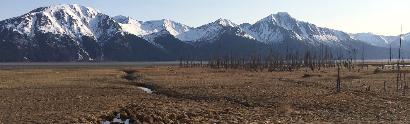
- This is a photo that I took along the Seward HWY 1, that runs east of Anchorage along the Turnagain Arm. I attended the 2014 Seismological Society of America Meeting that was located in Anchorage to commemorate the anniversary of the Good Friday Earthquake. This is a ghost forest of trees that perished as a result of coseismic subsidence during the earthquake. Copyright Jason R. Patton (2014). (Please contact me for a higher resolution version of this image: quakejay at gmail.com)
- Below is an educational video from the USGS that presents material about subduction zones and the 1964 earthquake and tsunami in particular.
Youtube Source IRIS - Animation & graphics by Jenda Johnson, geologist
- Directed by Robert F. Butler, University of Portland
- U.S. Geological Survey consultants: Robert C. Witter, Alaska Science Center Peter J. Haeussler, Alaska Science Center
- Narrated by Roger Groom, Mount Tabor Middle School
WMV file for downloading.
mp4 file for downloading.
-
Credits:
- Here is a map for the earthquakes of magnitude greater than or equal to M 7.0 between 1900 and 2016. This is the USGS query that I used to make this map. One may locate the USGS web pages for all the earthquakes on this map by following that link.
Some Relevant Discussion and Figures
- In june 2017, there was an M 6.8 earthquake that happened in a region where the Pacific-North America plate boundary transitions from a subduction zone to a shear zone. To the east of this region, the Pacific plate subducts beneath the North America plate to form the Alaska-Aleutian subduction zone. As a result of this subduction, a deep oceanic trench is formed. To the west of this earthquake, the plate boundary is in the form of a shear zone composed of several strike-slip faults. The main fault that is positioned in the trench is the Bering-Kresla shear zone (BKSZ), a right-lateral strike-slip fault. In the oceanic basin to the north of the BKSZ there are a series of parallel fracture zones, also right-lateral strike-slip faults. Below are my thoughts, some from my Earthquake Report here.
- My initial thought is that the entire Aleutian trench was a subduction zone prior to about 47 million years ago (Wilson, 1963; Torsvik et al., 2017). Prior to 47 Ma, the relative plate motion in the region of the BKSZ would have been more orthogonal (possibly leading to subduction there). After 47 Ma, the relative plate motion in the region of the BKSZ has been parallel to the plate boundary, owing to the strike-slip motion here. However, Konstantinovskaia (2001) used paleomagnetic data for a plate motion reconstruction through the Cenozoic and they have concluded that there is a much more complicated tectonic history here (with strike-slip faults in the region prior to 47 Ma and other faults extending much farther east into the plate boundary). When considering this, I was reminded that the relative plate motion in the central Aleutian subduction zone is oblique. This results in strain partitioning where the oblique motion is partitioned into fault-normal fault movement (subduction) and fault-parallel fault movement (strike-slip, along forearc sliver faults). The magmatic arc in the central Aleutian subduction zone has a forearc sliver fault, but also appears to have blocks that rotate in response to this shear (Krutikov, 2008).
- There have been several other M ~6 earthquakes to the west that are good examples of this strike-slip faulting in this area. On 2003.12.05 there was a M 6.7 earthquake along the Bering fracture zone (the first major strike-slip fault northeast of the BKSZ). On 2016.09.05 there was a M 6.3 earthquake also on the Bering fracture zone. Here is my earthquake report for the 2016 M 6.3 earthquake. The next major strike-slip fault, moving away from the BKSZ, is the right-lateral Alpha fracture zone. The M 6.8 earthquake may be related to this northwest striking fracture zone. However, aftershocks instead suggest that this M 6.8 earthquake is on a fault oriented in the northeast direction. There is no northeast striking strike-slip fault mapped in this area and the Shirshov Ridge is mapped as a thrust fault (albeit inactive). There is a left-lateral strike-slip fault that splays off the northern boundary of Bowers Ridge. If this fault strikes a little more counter-slockwise than is currently mapped at, the orientation would match the fault plane solution for this M 6.8 earthquake (and also satisfies the left-lateral motion for this orientation). The bathymetry used in Google Earth does not reveal the orientation of this fault, but the aftershocks sure align nicely with this hypothesis.
- I include some inset figures in the poster
- In the upper right corner is a figure that shows the historic earthquake ruptures along the Aleutian Megathrust (Peter Haeussler, USGS). I place a yellow star in the general location of this earthquake sequence (same for other figures here).
- In the upper left corner is a figure from Gaedicke et al. (2000) which shows some of the major tectonic faults in this region.
- In the lower right corner is a figure from Konstantnovskaia et al. (2001) that shows a very detailed view of all the faults in this complicated region.
- Here is the interpretive poster from the 2016.09.05 M 6.3 #EarthquakeReport.
- Here are several figures from Gaedicke et al. (2000) showing their tectonic reconstructions. I include their figure captions below in blockquote. The first map shows the general tectonic setting as in the poster above.
- This figure shows the complicated intersection of the BKSZ and the Kuril-Kamchatka Trench (a subduction zone).
- This figure shows a medium scale view of the faults here, along with the major historic earthquakes. In this figure the BKSZ is labeled the Aleutian fracture zone (AFZ).

Map of the Aleutian–Bering region and location of the study area (rectangle). Lines with barbs indicate subduction zones: (1) Kamchatka Trench and (2) Aleutian Trench; lines with sense of displacement mark fracture zones (FZs): (3) Steller, (4) Pikezh and (5) Bering FZs. Single arrows show relative direction of convergence of the Pacific (P) and North American (NA) plates. Bathymetric contours are in meters.

The main tectonic features of the Kamchatka–Aleutian junction area modified from Seliverstov (1983), Seliverstov et al. (1988) and Baranov et al. (1991). The eastern side of the Central Kamchatka depression is bounded by normal faults. Contour interval is 1000 m. Lines A and B indicate the locations of profiles shown in Fig. 3; the rectangle marks the location of the area shown in Fig. 4.

Rupture zones of the major earthquakes in the Kamchatka–Aleutian junction area [according to Vikulin (1997)]. Earthquakes with a magnitude of Mw>7 are shown.
- Here is a great illustration that shows how forearc sliver faults form due to oblique convergence at a subduction zone (Lange et al., 2008). Strain is partitioned into fault normal faults (the subduction zone) and fault parallel faults (the forearc sliver faults, which are strike-slip). This figure is for southern Chile, but is applicable globally.

Proposed tectonic model for southern Chile. Partitioning of the oblique convergence vector between the Nazca plate and South American plate results in a dextral strike-slip fault zone in the magmatic arc and a northward moving forearc sliver. Modified after Lavenu and Cembrano (1999).
- Here is a figure from Krutikov (2008) showing the block rotation and forearc sliver faults associated with the oblique subduction in the central Aleutian subduction zone. Note that there are blocks that are rotating to accommodate the oblique convergence. There are also margin parallel strike slip faults that bound these blocks. These faults are in the upper plate, but may impart localized strain to the lower plate, resulting in strike slip motion on the lower plate (my arm waving part of this). Note how the upper plate strike-slip faults have the same sense of motion as these deeper earthquakes.

- Here are several figures from Konstantnovskaia et al. (2001) showing their tectonic reconstructions. I include their figure captions below in blockquote. The first figure is the one included in the poster above.
- Here are 4 panels that show the details of their reconstructions. Panels shown are for 65 Ma, 55 Ma, 37 Ma, and Present.

Geodynamic setting of Kamchatka in framework of the Northwest Pacific. Modified after Nokleberg et al. (1994) and Kharakhinov (1996)). Simplified cross-section line I-I’ is shown in Fig. 2. The inset shows location of Sredinny and Eastern Ranges. [More figure caption text in the publication].


The Cenozoic evolution in the Northwest Pacific. Plate kinematics is shown in hotspot reference frame after (Engebretson et al., 1985). Keys distinguish zones of active volcanism (thick black lines), inactive volcanic belts (thick gray lines), deformed arc terranes (hatched pattern), subduction zones: active (black triangles), inactive *(empty triangles). In letters: sa = Sikhote-aline, bs = Bering shelf belts; SH = Shirshov Ridge; V = Vitus arch; KA = Kuril; RA = Ryukyu’ LA = Luzon; IBMA = Izu-Bonin-Mariana arcs; WPB = Western Philippine, BB = Bowers basins.
- On 2017.05.08 there was an earthquake further to the east, with a magnitude M 6.2. Here is my interpretive poster for this earthquake, which includes fault plane solutions for several historic earthquakes in the region. These fault plane solutions reveal the complicated intersection of these two different types of faulting along this plate boundary. Here is my earthquake report for this earthquake sequence.
- Here is the figure from Bassett and Watts (2015) for the Aleutians. They use gravity profile data to characterize subduction zones globally.

Aleutian subduction zone. Symbols as in Figure 3. (a) Residual free-air gravity anomaly and seismicity. The outer-arc high, trench-parallel fore-arc ridge and block-bounding faults are dashed in blue, black, and red, respectively. Annotations are AP = Amchitka Pass; BHR = Black-Hills Ridge; SS = Sunday Sumit Basin; PD = Pratt Depression. (b) Published asperities and slip-distributions/aftershock areas for large magnitude earthquakes. (c) Cross sections showing residual bathymetry (green), residual free-air gravity anomaly (black), and the geometry of the seismogenic zone [Hayes et al., 2012].
- Here is the schematic figure from Bassett and Watts (2015).

Schematic diagram summarizing the key spatial associations interpreted between the morphology of the fore-arc and variations in the seismogenic behavior of subduction megathrusts.
- Here is a beautiful illustration for the Aleutian Trench from Alpha (1973) as posted on the David Rumsey Collection online.

- Here is the figure from Sykes et al. (1980) that shows the space time relations for historic earthquakes in relation to the map.

Above: Rupture zones of earthquakes of magnitude M > 7.4 from 1925-1971 as delineated by their aftershocks along plate boundary in Aleutians, southern Alaska and offshore British Columbia [after Sykes, 1971]. Contours in fathoms. Various symbols denote individual aftershock sequences as follows: crosses, 1949, 1957 and 1964; squares, 1938, 1958 and 1965; open triangles, 1946; solid triangles, 1948; solid circles, 1929, 1972. Larger symbols denote more precise locations. C = Chirikof Island. Below: Space-time diagram showing lengths of rupture zones, magnitudes [Richter, 1958; Kanamori, 1977 b; Kondorskay and Shebalin, 1977; Kanamori and Abe, 1979; Perez and Jacob, 1980] and locations of mainshocks for known events of M > 7.4 from 1784 to 1980. Dashes denote uncertainties in size of rupture zones. Magnitudes pertain to surface wave scale, M unless otherwise indicated. M is ultra-long period magnitude of Kanamori 1977 b; Mt is tsunami magnitude of Abe[ 1979]. Large shocks 1929 and 1965 that involve normal faulting in trench and were not located along plate interface are omitted. Absence of shocks before 1898 along several portions of plate boundary reflects lack of an historic record of earthquakes for those areas.
- This is a map from Sykes et al. (1980) that shows the regions of slip inferred for these historic earthquakes.
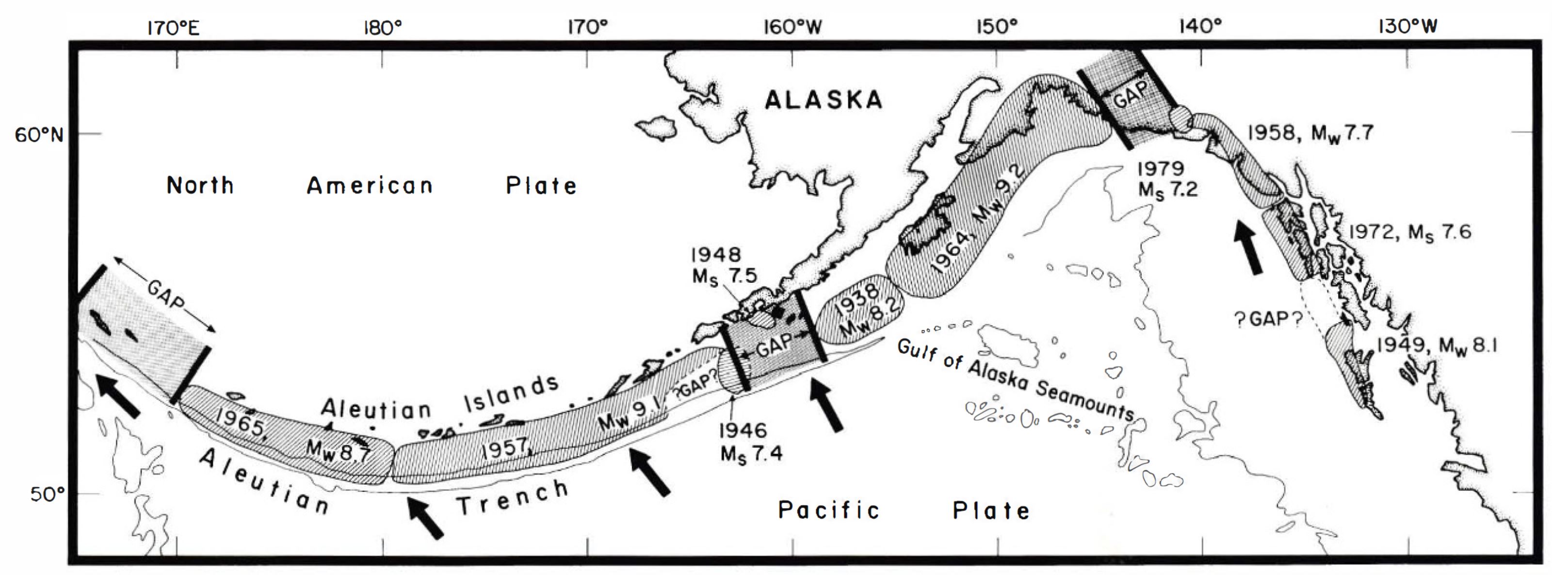
Aftershock areas of earthquakes of magnitude M > 7.4 in the Aleutians, southern Alaska and offshore British Columbia from 1938 to 1979, after Sykess [1971] and McCann et al. [1979]. Heavy arrows denote motion of Pacific plate with respect to North American plate as calculated by Chase [1978]. Two thousand fathom contour is shown for Aleutian trench. Ms and Mw denote magnitude scales described by Kanamori [1977b].
Geologic Fundamentals
- For more on the graphical representation of moment tensors and focal mechnisms, check this IRIS video out:
- Here is a fantastic infographic from Frisch et al. (2011). This figure shows some examples of earthquakes in different plate tectonic settings, and what their fault plane solutions are. There is a cross section showing these focal mechanisms for a thrust or reverse earthquake. The upper right corner includes my favorite figure of all time. This shows the first motion (up or down) for each of the four quadrants. This figure also shows how the amplitude of the seismic waves are greatest (generally) in the middle of the quadrant and decrease to zero at the nodal planes (the boundary of each quadrant).

- Here is another way to look at these beach balls.
The two beach balls show the stike-slip fault motions for the M6.4 (left) and M6.0 (right) earthquakes. Helena Buurman's primer on reading those symbols is here. pic.twitter.com/aWrrb8I9tj
— AK Earthquake Center (@AKearthquake) August 15, 2018
- There are three types of earthquakes, strike-slip, compressional (reverse or thrust, depending upon the dip of the fault), and extensional (normal). Here is are some animations of these three types of earthquake faults. The following three animations are from IRIS.
Strike Slip:
Compressional:
Extensional:
- This is an image from the USGS that shows how, when an oceanic plate moves over a hotspot, the volcanoes formed over the hotspot form a series of volcanoes that increase in age in the direction of plate motion. The presumption is that the hotspot is stable and stays in one location. Torsvik et al. (2017) use various methods to evaluate why this is a false presumption for the Hawaii Hotspot.
- Here is a map from Torsvik et al. (2017) that shows the age of volcanic rocks at different locations along the Hawaii-Emperor Seamount Chain.

A cutaway view along the Hawaiian island chain showing the inferred mantle plume that has fed the Hawaiian hot spot on the overriding Pacific Plate. The geologic ages of the oldest volcano on each island (Ma = millions of years ago) are progressively older to the northwest, consistent with the hot spot model for the origin of the Hawaiian Ridge-Emperor Seamount Chain. (Modified from image of Joel E. Robinson, USGS, in “This Dynamic Planet” map of Simkin and others, 2006.)

Hawaiian-Emperor Chain. White dots are the locations of radiometrically dated seamounts, atolls and islands, based on compilations of Doubrovine et al. and O’Connor et al. Features encircled with larger white circles are discussed in the text and Fig. 2. Marine gravity anomaly map is from Sandwell and Smith.
- Summary of the 1964 Earthquake
- 2018.08.15 M 6.6 Aleutians
- 2018.08.12 M 6.4 North Alaska
- 2018.01.23 M 7.9 Gulf of Alaska
- 2018.01.23 M 7.9 Gulf of Alaska UPDATE #1
- 2018.01.23 M 7.9 Gulf of Alaska UPDATE #2
- 2017.07.17 M 7.7 Aleutians
- 2017.07.17 M 7.7 Aleutians UPDATE #1
- 2017.06.02 M 6.8 Aleutians
- 2017.05.08 M 6.2 Aleutians
- 2017.05.01 M 6.3 British Columbia
- 2017.03.29 M 6.6 Kamchatka
- 2017.03.02 M 5.5 Alaska
- 2016.09.05 M 6.3 Bering Kresla (west of Aleutians)
- 2016.04.13 M 5.7 & 6.4 Kamchatka
- 2016.04.02 M 6.2 Alaska Peninsula
- 2016.03.27 M 5.7 Aleutians
- 2016.03.12 M 6.3 Aleutians
- 2016.01.29 M 7.2 Kamchatka
- 2016.01.24 M 7.1 Alaska
- 2015.11.09 M 6.2 Aleutians
- 2015.11.02 M 5.9 Aleutians
- 2015.11.02 M 5.9 Aleutians (update)
- 2015.07.27 M 6.9 Aleutians
- 2015.05.29 M 6.7 Alaska Peninsula
- 2015.05.29 M 6.7 Alaska Peninsula (animations)
- 1964.03.27 M 9.2 Good Friday
Alaska | Kamchatka | Kurile Earthquake Reports
General Overview
Earthquake Reports
Social Media
Today in "Alaska is really big": Sunday's magnitude 6.4 earthquake in the northern Brooks Range and today's magnitude 6.6 earthquake in the Andreanof Islands occurred over 1,600 miles apart. pic.twitter.com/mfyfxdJfpr
— AK Earthquake Center (@AKearthquake) August 15, 2018
These seismic waves (generated by a M6.6 earthquake near the Aleutian Islands) rolled through #Victoria a few minutes ago…
Not felt, but easily recorded by our seismograph on Gonzales Hill.
Details on this Alaska earthquake: https://t.co/FxCCohDiK3 pic.twitter.com/JbjmfYkOjU— John Cassidy (@earthquakeguy) August 15, 2018
- Abe, K., 1972. Lithospheric Normal Faulting Beneath the Aleutian Trench in Phys. Earth Planet. Interiors, v. 5, p. 1990-198.
- Bassett and Watts, 2015 A. Gravity anomalies, crustal structure, and seismicity at subduction zones: 1. Seafloor roughness and subducting relief in Geochemistry, Geophysics, Geosystems, v. 16, doi:10.1002/2014GC005684.
- Bassett, D. and Watts, A.B., 2015 B. Gravity anomalies, crustal structure, and seismicity at subduction zones: 2. Interrelationships between fore-arc structure and seismogenic behavior in Geochemistry, Geophysics, Geosystems, v. 16, doi:10.1002/2014GC005685.
- Brown, J.R., Prejan, S.G., Beroza, G.C., Gomberg, J.S., and Hauessler,m P.J., 2013. Deep low-frequency earthquakes in tectonic tremor along the Alaska-Aleutian subduction zone in JGR Solid Earth, v. 118, p. 1079-1090, doi:10.1029/2012JB009459
- Ikuta, R., Mitsui, Y., Kurokawa, Y., and Ando, M., 2015. Evaluation of strain accumulation in global subduction zones from seismicity data in Earth, Planets and Space, v. 67, DOI 10.1186/s40623-015-0361-5
- Lay, T., H. Kanamori, C. J. Ammon, A. R. Hutko, K. Furlong, and L. Rivera, 2009. The 2006 – 2007 Kuril Islands great earthquake sequence in J. Geophys. Res., 114, B11308, doi:10.1029/2008JB006280.
- Hayes, G.P., Wald, D.J., and Johnson, R.L., 2012. Slab1.0: A three-dimensional model of global subduction zone geometries in, J. Geophys. Res., 117, B01302, doi:10.1029/2011JB008524
- Meyer, B., Saltus, R., Chulliat, a., 2017. EMAG2: Earth Magnetic Anomaly Grid (2-arc-minute resolution) Version 3. National Centers for Environmental Information, NOAA. Model. doi:10.7289/V5H70CVX
- Gaedicke, C., Baranov, B., Seliverstov, N., Alexeiev, D., Tsukanov, N., Freitag, R., 2000. Structure of an active arc-continent collision area: the Aleutian-Kamchatka junction. Tectonophysics 325, 63–85
- Hayes, G. P., D. J. Wald, and R. L. Johnson, 2012. Slab1.0: A three-dimensional model of global subduction zone geometries, J. Geophys. Res., 117, B01302, doi:10.1029/2011JB008524.
- Koulakov, I.Y., Dobretsov, N.L., Bushenkova, N.A., and Yakovlev, A.V., 2011. Slab shape in subduction zones beneath the Kurile–Kamchatka and Aleutian arcs based on regional tomography results in Russian Geology and Geophysics, v. 52, p. 650-667.
- Konstantnovskaia, 2001. Arc-continent collision and subduction reversal in the Cenozoic evolution of the Northwest Pacific: an example from Kamchatka (NE Russia) in Tectonophysics, v. 333, p. 75-94.
- Krutikov, L., Stone, D.B., and Minyuk, P., 2008. New Paleomagnetic Data From the Central Aleutian Arc: Evidence and Implications for Block Rotations in Active Tectonics and Seismic Potential of Alaska, Geophysical Monograph Series 179 American Geophysical Union. 10.1029/179GM07
- Lange, D., Cembrano, J., Rietbrock, A., Haberland, C., Dahm, T., and Bataille, K., 2008. First seismic record for intra-arc strike-slip tectonics along the Liquiñe-Ofqui fault zone at the obliquely convergent plate margin of the southern Andes in Tectonophysics, v. 455, p. 14-24
- Plafker, G., 1972. Alaskan earthquake of 1964 and Chilean earthquake of 1960: Implications for arc tectonics in Journal of Geophysical Research, v. 77, p. 901-925.
- Portnyagin, M. and Manea, V.C., 2008. Mantle temperature control on composition of arc magmas along the Central Kamchatka Depression in Geology, v. 36, no. 7, p. 519-522.
- Rhea, S., Tarr, A.C., Hayes, G., Villaseñor, A., Furlong, K.P., and Benz, H.M., 2010. Seismicity of the Earth 1900-2007, Kuril-Kamchatka arc and vicinity: U.S. Geological Survey Open-File Report 2010-1083-C, 1 map sheet, scale 1:5,000,000.
- Saltus, R.W., and Barnett, A., 2000. Eastern Aleutian Volcanic Arc Digital Model – Version 1.0: U.S. Geological Survey Open-File Report 00
- Stauyder, W., 1968. Mechanism of the Rat Island Earthquake Sequence of February 4, 1965, with Relation to Island Arcs and Sea-Floor Spreading in JGR, v. 73, no. 12, p. 3847-3858
- Sykes, L.R., Kissinger, J.B>, House, L., Davies, J.N>, and Jacob, K.H., 1980. Rupture Zones and Repeat Times of Great Earthquakes Along the Alaska-Aleutian Arc, 1784-1980, in Maurice Ewing Series, Earthquake Prediction, An International Review, AGU
- Torsvik, T. H. et al., 2017. Pacific plate motion change caused the Hawaiian-Emperor Bend in Nat. Commun., v. 8, doi: 10.1038/ncomms15660
- Wilson, J. Tuzo, 1963. “A possible origin of the Hawaiian Islands” in Canadian Journal of Physics. v. 41, p. 863–870 doi:10.1139/p63-094.
References:
°
≥