Well, around 3 AM my time (northeastern Pacific, northern CA) there was a sequence of earthquakes including a mainshock with a magnitude M = 7.5. This earthquake happened in a highly populated region of Indonesia.
This area of Indonesia is dominated by a left-lateral (sinistral) strike-slip plate boundary fault system. Sulawesi is bisected by the Palu-Kola / Matano fault system. These faults appear to be an extension of the Sorong fault, the sinistral strike-slip fault that cuts across the northern part of New Guinea.
There have been a few earthquakes along the Palu-Kola fault system that help inform us about the sense of motion across this fault, but most have maximum magnitudes mid M 6.
GPS and block modeling data suggest that the fault in this area has a slip rate of about 40 mm/yr (Socquet et al., 2006). However, analysis of offset stream channels provides evidence of a lower slip rate for the Holocene (last 12,000 years), a rate of about 35 mm/yr (Bellier et al., 2001). Given the short time period for GPS observations, the GPS rate may include postseismic motion earlier earthquakes, though these numbers are very close.
Using empirical relations for historic earthquakes compiled by Wells and Coppersmith (1994), Socquet et al. (2016) suggest that the Palu-Koro fault system could produce a magnitude M 7 earthquake once per century. However, studies of prehistoric earthquakes along this fault system suggest that, over the past 2000 years, this fault produces a magnitude M 7-8 earthquake every 700 years (Bellier et al., 2006). So, it appears that this is the characteristic earthquake we might expect along this fault.
Based on what we know about strike-slip fault earthquakes, the portions of the fault to the north and south of today’s sequence may have an increased amount of stress due to this earthquake. Stay tuned for a Temblor.net report about this earthquake where I discuss this further.
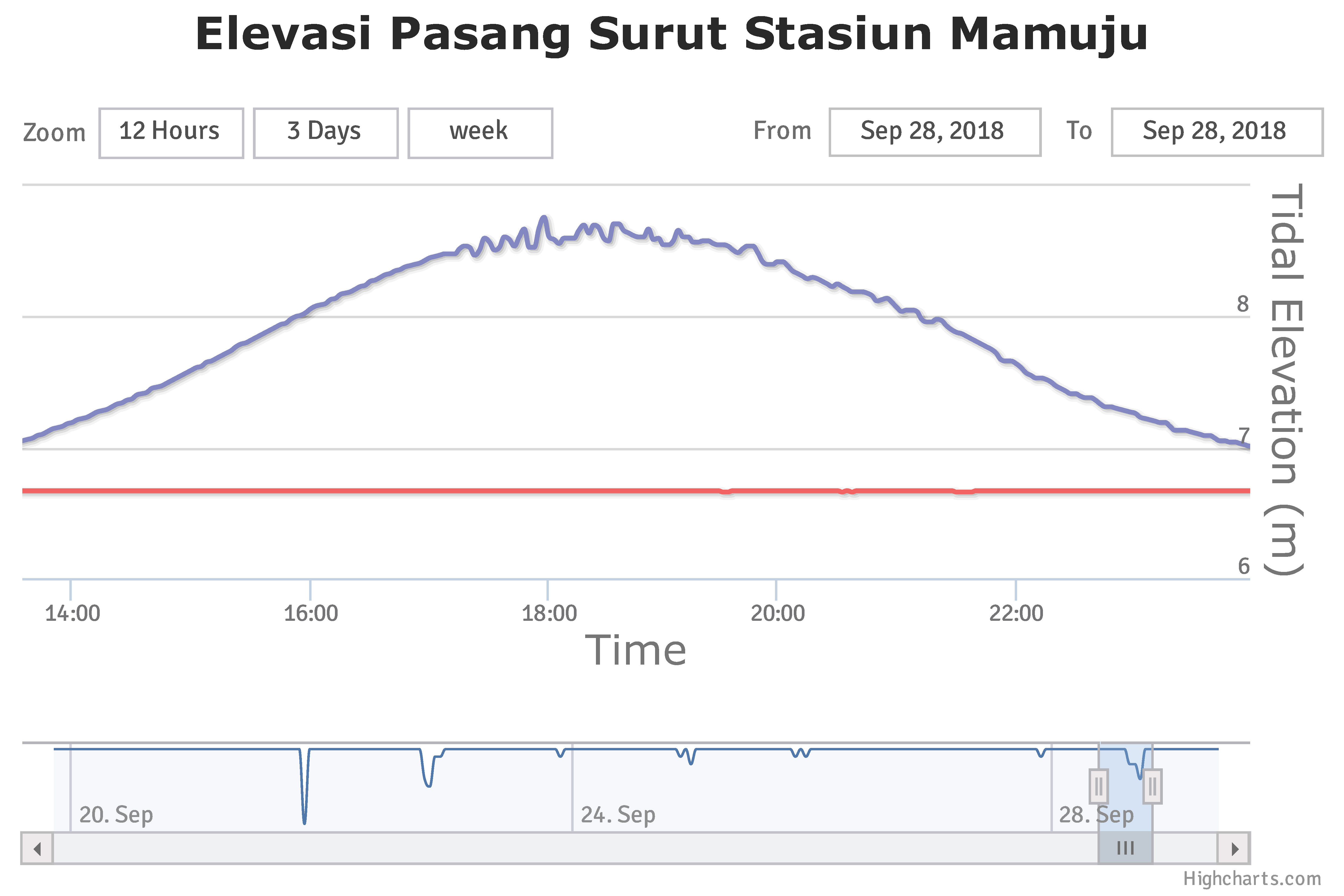
There are reports of a local tsunami with a run-up about 2 meters. However, the UNESCO Sea Level Monitoring Facility (website) does not show any tsunami observations on tide gage data in the region.
Most commonly, we associate tsunamigenic earthquakes with subduction zones and thrust faults because these are the types of earthquakes most likely to deform the seafloor, causing the entire water column to be lifted up. Strike-slip earthquakes can generate tsunami if there is sufficient submarine topography that gets offset during the earthquake. Also, if a strike-slip earthquake triggers a landslide, this could cause a tsunami. We will need to wait until people take a deeper look into this before we can make any conclusions about the tsunami and what may have caused it.
Did you feel this earthquake? If so, fill out the USGS “Did You Feel It?” form here. If not, why not? Probably because you were too far away. The closer to an earthquake, the more strong the shaking intensity and the larger chance of infrastructure damage (roads, houses, etc.). The USGS PAGER alert for this earthquake shows that there are ~282,000 people living in Palu, a city near the epicenter. The estimate for shaking intensity is a MMI VI, which could result in light damage for resistant structures and moderate damage for vulnerable structures. More about USGS PAGER alerts here. There exists a possibility that there were more than 100 fatalities from this earthquake.
UPDATE 2018.09.28 23:00
- There have been tsunami waves recorded on a tide gage over 300 km to the south of the epicenter, at a site called Mumuju. Below is a map and a plot of water surface elevations from this source.

UPDATE 2018.09.29 07:00
I awakened this morning (my time, obviously) to find that there are over 380 reported deaths from this earthquake and tsunami. More on this later in the day (clouds are preparing to our and i need to put some of my stuff under tarps).
I prepared a report for Temblor where we present results of static coulomb stress modeling. Here is that report.
UPDATE 2018.09.29 10:45
Here is a (200 MB) video that I edited slightly. Download here. This was originally posted here.
UPDATE 2018.09.30 17:00
- I was interviewed by Henry Fountain (NYT) today. Here is the story he wrote.
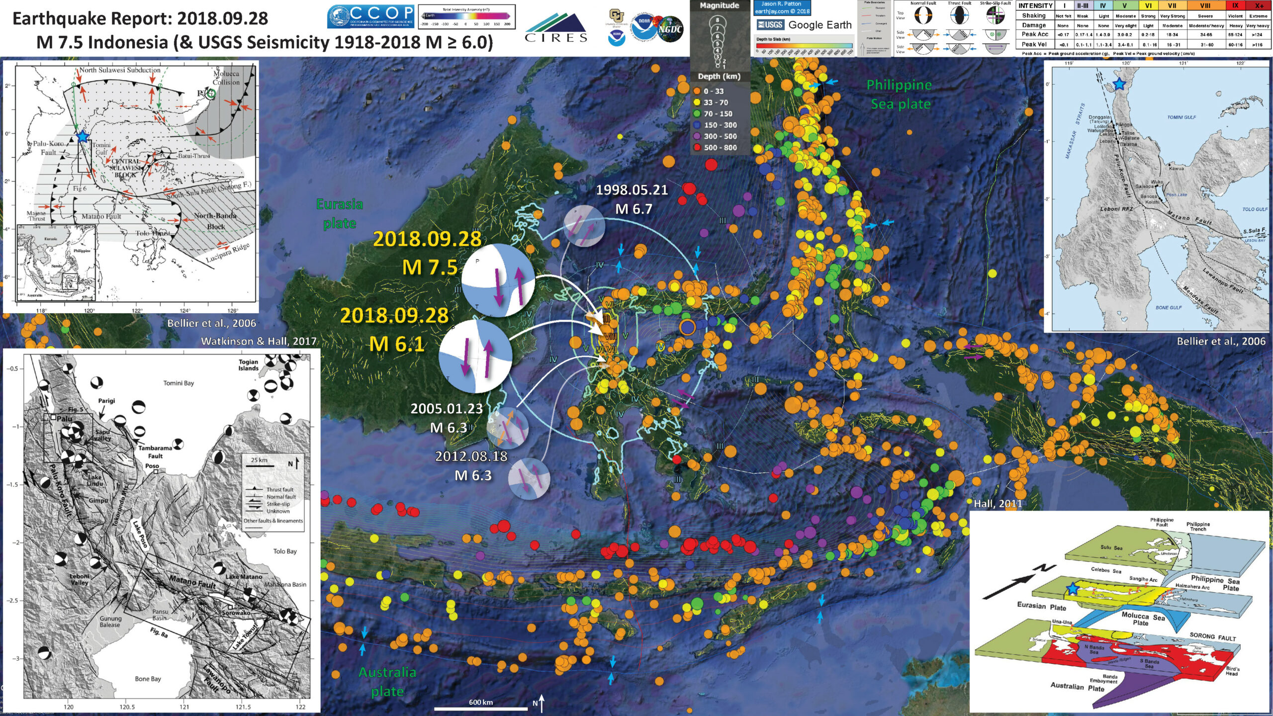
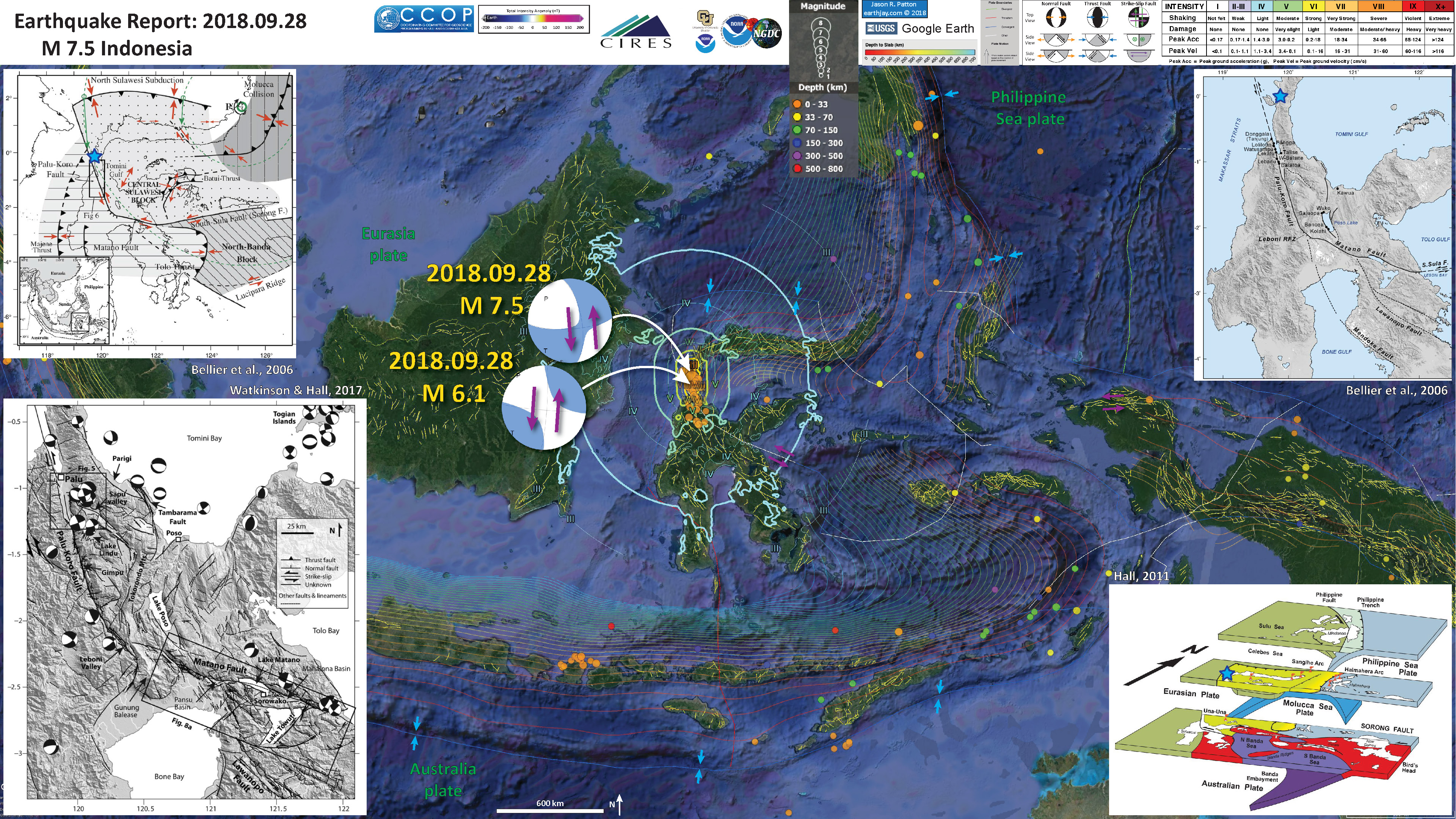
Below is my interpretive poster for this earthquake
I plot the seismicity from the past month, with color representing depth and diameter representing magnitude (see legend). I include earthquake epicenters from 1918-2018 with magnitudes M ≥ 6.0 in one version.
I plot the USGS fault plane solutions (moment tensors in blue and focal mechanisms in orange), possibly in addition to some relevant historic earthquakes.
- I placed a moment tensor / focal mechanism legend on the poster. There is more material from the USGS web sites about moment tensors and focal mechanisms (the beach ball symbols). Both moment tensors and focal mechanisms are solutions to seismologic data that reveal two possible interpretations for fault orientation and sense of motion. One must use other information, like the regional tectonics, to interpret which of the two possibilities is more likely.
- I also include the shaking intensity contours on the map. These use the Modified Mercalli Intensity Scale (MMI; see the legend on the map). This is based upon a computer model estimate of ground motions, different from the “Did You Feel It?” estimate of ground motions that is actually based on real observations. The MMI is a qualitative measure of shaking intensity. More on the MMI scale can be found here and here. This is based upon a computer model estimate of ground motions, different from the “Did You Feel It?” estimate of ground motions that is actually based on real observations.
- I include the slab 2.0 contours plotted (Hayes, 2018), which are contours that represent the depth to the subduction zone fault. These are mostly based upon seismicity. The depths of the earthquakes have considerable error and do not all occur along the subduction zone faults, so these slab contours are simply the best estimate for the location of the fault.
- In the map below, I include a transparent overlay of the magnetic anomaly data from EMAG2 (Meyer et al., 2017). As oceanic crust is formed, it inherits the magnetic field at the time. At different points through time, the magnetic polarity (north vs. south) flips, the north pole becomes the south pole. These changes in polarity can be seen when measuring the magnetic field above oceanic plates. This is one of the fundamental evidences for plate spreading at oceanic spreading ridges (like the Gorda rise).
- Regions with magnetic fields aligned like today’s magnetic polarity are colored red in the EMAG2 data, while reversed polarity regions are colored blue. Regions of intermediate magnetic field are colored light purple.
- We can see the roughly east-west trends of these red and blue stripes. These lines are parallel to the ocean spreading ridges from where they were formed. The stripes disappear at the subduction zone because the oceanic crust with these anomalies is diving deep beneath the Sunda plate (part of Eurasia), so the magnetic anomalies from the overlying Sunda plate mask the evidence for the Australia plate.
Magnetic Anomalies
- In the upper left corner is a map from Bellier et al. (2016) that shows the plate boundary faults in the region. Relative senses of motion across these faults is shown as red arrows. The M 7.5 epicenter is shown as a blue star (as in other figures).
- In the upper right corner is a larger scale map showing the strike-slip fautls that transect the island of Sulawesi, Indonesia (Bellier, et al., 2006)
- In the lower right corner is a low angle oblique view of the subducting plates in this region (Hall, 2011). Note the orientation of the Sorong fault and the Sulawesi faults.
- In the lower left corner is a large scale map showing detailed versions of these fault systems in Sulawesi. Earthquake fault mechanisms are plotted for historic earthquakes. Today’s M 7.5 occurred just to the north of the spatial extent of this map.
I include some inset figures. Some of the same figures are located in different places on the larger scale map below.
- Here is the map with a month’s seismicity plotted.
- Here is the map with a centuries worth of seismicity plotted.

Other Report Pages
- The official press release from the Meteorology Climatology and Geophysics Council is here.
- earthquake report dot com
- Dr. Erik Klemetti Discover Magazine
Some Relevant Discussion and Figures
- Here is the low angle oblique view of the plate boundaries in this region (Hall., 2011).

3D cartoon of plate boundaries in the Molucca Sea region modified from Hall et al. (1995). Although seismicity identifies a number of plates there are no continuous boundaries, and the Cotobato, North Sulawesi and Philippine Trenches are all intraplate features. The apparent distinction between different crust types, such as Australian continental crust and oceanic crust of the Philippine and Molucca Sea, is partly a boundary inactive since the Early Miocene (east Sulawesi) and partly a younger but now probably inactive boundary of the Sorong Fault. The upper crust of this entire region is deforming in a much more continuous way than suggested by this cartoon.
- Here is the seismic hazard map from the Indonesian National Agency for Disaster Management (2011). This is the full map, for which a subset is included in the interpretive poster above.

- Here is the map from Bellier et al. (2006) that shows the plate boundary faults, along with some other tectonic information.

Regional geodynamic sketch that presents the present day deformation model of Sulawesi area (after Beaudouin et al., 2003) and four main deformation systems around the Central Sulawesi block, highlighting the tectonic complexity of Sulawesi. Approximate location of the Central Sulawesi block rotation pole (P) [compatible with both GPS measurements (Walpersdorf et al., 1998a) and earthquake moment tensor analyses (Beaudouin et al., 2003)], as well as the major active structures are reported. Central Sulawesi Fault System (CSFS) is formed by the Palu–Koro and Matano faults. Arrows correspond to the compression and/or extension directions deduced from both inversion and moment tensor analyses of the focal mechanisms; arrow size being proportional to the deformation rate (e.g., Beaudouin et al., 2003).We also represent the focal mechanism provided by the Harvard CMT database [CMT data base, 2005] for the recent large earthquake (Mw=6.2; 2005/1/23; lat.=0.92° S; long.=120.10° E). The box indicates the approximate location of the Fig. 6 that corresponds to the geological map of the Palu basin region. The bottom inset shows the SE Asia and Sulawesi geodynamic frame where arrows represent the approximate Indo-Australian and Philippines plate motions relative to Eurasia.
- The is the larger scale map showing the general layout of the strike-slip faults in Sulawesi (Bellier et al., 2006).
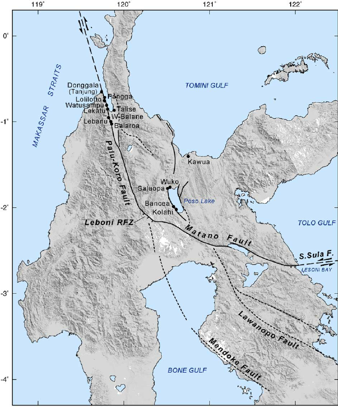
Sketch map of the Cenozoic Central Sulawesi fault system. ML represents the Matano Lake, and Leboni RFZ, the Leboni releasing fault zone that connects the Palu–Koro and Matano Faults. Triangles indicate faults with reverse component (triangles on the upthrown block). On this map are reported the fault kinematic measurement sites.
- Here is a spectacular photo/sketch pair that demonstrates the excellent geomorphic evidence for this strike-slip fault (Bellier et al., 2006).The stream channels that flow down the alluvial fan in this photo are typical of the features that were used to evaluate the Holocene slip rate. There is a modest amount of vertical motion across this fault in places, causing the formation of basins like the Palu Palu Basin (a graben). The city of Palu is in the center of the Palu Palu Basin.
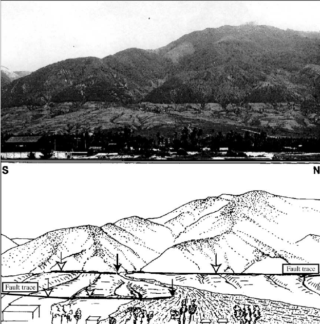
West-looking view of the Palu–Koro fault escarpment SSW of the Palu basin showing faceted spurs and a left-lateral offset of an alluvial fan. At the bottom, sketch of the photograph where white arrows point to the fault trace and black arrows point to the cumulate fan offset along the fault traces.
- This map shows how Palu is situated relative to this fault system (Bellier et al., 2006).
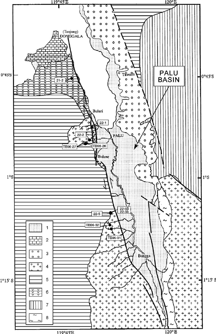
Simplified geological map of the Palu domain (modified after Sukamto, 1973) where are reported the locations of fission-track samples. 1 — Holocene alluvial deposits; 2 — Quaternary coral reef terraces; 3 — Mio-quaternary molasses, 4 — Mio-quaternary granitic rocks and granodiorites, 5 — Middle to Upper Eocene Tinombo Formation metamorphism, 6 — Tinombo Formation magmatism, 7 and 8 — metamorphic bedrock (7 — Cretaceous Latimonjong Formation; 8 — Triassic-Jurassic Gumbasa Formation).
- Some early GPS analysis was conducted by Waldpersdorf et al. (1998). Below is a map showing the location of these GPS observations relative tot he Palu-Koro fault.

The area of convergence of the Eurasian, Philippine and Australian plate is characterized by the Sula block motion. Active block boundaries are the North Sulawesi trench *(1)., the Palu-Koro (2), and the Matano (3) faults. The Palu transect is indicated buy the box, with a zoom presented in the inset. Furthermore, the two largest earthquakes (CMT) occurring during the observation period are indicated.
- Here is a map that shows the GPS velocities as vectors in the region of Palu, Indonesia (Waldpersdorf et al., 1998).

Velocities of the Palu transect stations, with respect to the PALU station. Error ellipses correspond to formal uncertainties of the global solution with a confidence level of 90%.
- Here are the Waldpersdorf et al. (1998) velocities plotted on a chart.
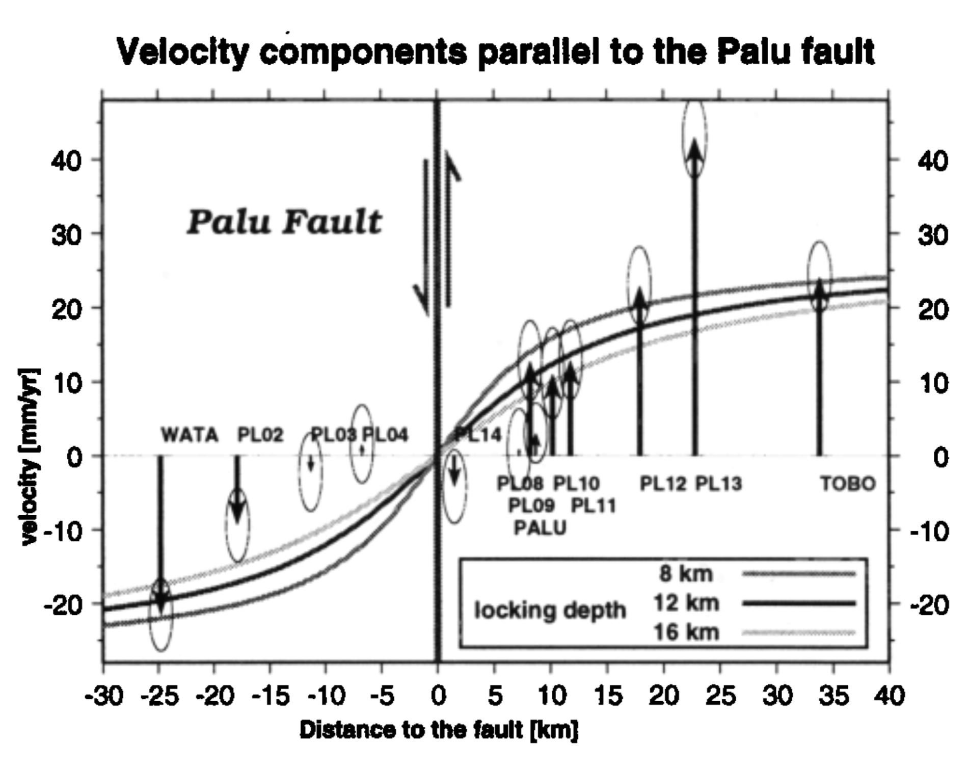
Transect station velocity components parallel to the fault, with the co-seismic deformation due to the Jan. 1996 earthquake removed. They are indicated in function of their distance to the fault. The dark grey line shows best model values (5.5 cm/yr total velocity, 12 km locking depth). Lighter grey lines correspond to locking depths of 8 and 16 km, marking an uncertainty of +-4 km.
- Below are updated results from GPS and block model analyses from Socquet et al. (2006). Arrows are vectors that represent plate motion velocity in mm/yr (scale in upper right corner). Note how the velocities are different on either side of the Palu-Koro fault.

GPS velocities of Sulawesi and surrounding sites with respect to the Sunda Plate. Grey arrows belong to the Makassar Block, black arrows belong to the northern half of Sulawesi, and white arrows belong to non-Sulawesi sites (99% confidence ellipses). Numbers near the tips of the vectors give the rates in mm/yr. The main tectonic structures of the area are shown as well.
- This map shows models plate motion velocities as informed by their block model.

Rotational part of the inferred velocity field in the Sulawesi area (relative to the Sunda Plate) as predicted by the Euler vectors of the best fit model (model 2). Error ellipses of predicted vectors show the 99% level of confidence. Also shown are poles of rotation and error ellipses (with respect to the Sunda Plate) from the best fit model. Curved arrows indicate the sense of rotation, and numbers indicate the rotation rate. MAKA, Makassar Block; MANA, Manado Block; ESUL, East Sula Block; NSUL, North Sula Block.
- Here is a map that shows the plate boundary slip velocities as color (Socquet et al., 2006).

Best fit block model derived from both GPS and earthquakes slip vector azimuth data. Center: Observed (red) and calculated (green) velocities with respect to the Sunda Block (shown are 20% confidence ellipses, after GPS reweighting; see text). The slip rate deficit (mm/yr) for the faults included in the model is represented by a color bar. The profile of Figure 7 is located by the dashed black line. The black rectangles around Palu and Gorontalo faults localize the insets. Top right and bottom left insets show details of the measured and modeled velocities across the Gorontalo and Palu faults. The bottom right inset shows residual GPS velocities with respect to the model. The value of the coupling ratio, j, for the faults included in the model is represented by the color bar. Light blue dots represent the locations of the fault nodes where the coupling ratio is estimated. Nodes along the block boundaries are at the surface of the Earth, and the others are at depth along the fault plane. In this model, j is considered uniform along strike and depth for all the faults, except for Palu Fault and Minahassa Trench, where it is allowed to vary along strike.
- This plot is similar to the one above, which shows how different GPS observations have different plate motion velocities relative to the faults in the area (Socquet et al., 2006).

Velocity profile across Makassar Trench, Palu Fault, and Gorontalo Fault (profile location in Figure 6) in Sunda reference frame. Observed GPS velocities are depicted by dots with 1-sigma uncertainty bars, while the predicted velocities are shown as curves. The profile normal component (approximately NNW) (i.e., the strike-slip component across the NW trending faults) is shown with black dots and solid line, while the profile-parallel component (normal or thrust component across the fault) is shown with grey dots and a dashed line. Where the profile crosses the faults and blocks is labeled.
- Here are their results plotted on a map (Socquet et al., 2006).

(top) GPS velocities in Palu area relative to station WATA. STRM topography is used as background. (bottom) Four parallel elastic dislocations that fit best the velocities in the Palu fault zone. The fault-parallel component of the GPS velocities (with 1-sigma error bars) is plotted with respect to their distance to the main fault scarp, in the North Sula Block reference frame. The black curve represents the fault-parallel modeled velocity of the four strand model. For comparison, the fault-parallel modeled velocity predicted by the single fault model is also plotted (grey dashed curve). The location of the modeled dislocation is represented as vertical bars for each model (black and dashed grey lines, respectively).
- Here is the fault map from Watkinson and Hall (2017).

Central Sulawesi overview digital elevation model (SRTM), CMT catalogue earthquakes, 35 km depth and structures that show geomorphic evidence of Quaternary tectonic activity. Rivers marked in white. Illumination from NE.
- Here is another fantastic view of the geomorphology associated with the Palu-Koro fault (Watkinson and Hall, 2017). The hanging valley is evidence for normal displacement (extension) along this fault. Wine glass canyons are evidence for differential uplift.

(a) The Palu and Sapu valleys showing structures that with geomorphic evidence of Quaternary tectonic activity, plus topography and drainage. Mountain front sinuosity values in bold italic text. For location, see Figure 4. Major drainage basins for Salo Sapu and Salo Wuno are marked, separated by uplift at the western end of the Sapu valley fault system. (b) View of the Palu–Koro Fault scarp from the Palu valley, showing geomorphic evidence of Quaternary tectonic activity.
- In this case, we can see how the river meanders are controlled by the fault. Places where stream offsets were used to measure slip rate are also shown (Watkinson and Hall, 2017).

Evidence of a cross-basin fault system within the Palu valley Quaternary fill. (a) Overview ASTER digital elevation model draped with ESRI imagery layer. Illumination from NW. Palu River channels traced from six separate images from 2003 to 2015. Inset shows fault pattern developed in an analogue model of a releasing bend, modified after Wu et al. (2009), reflected and rotated to mimic the Palu valley. Sidewall faults and cross-basin fault system are highlighted in the model and on the satellite imagery. (b, c) Laterally confined meander belts, interpreted as representing minor subsidence within the cross-basin fault system. (d) Laterally confined river channels directly along-strike from a Palu–Koro Fault strand seen to offset alluvial fans in the south of the valley. (c, d, e) showESRI imagery.
Geologic Fundamentals
- For more on the graphical representation of moment tensors and focal mechnisms, check this IRIS video out:
- Here is a fantastic infographic from Frisch et al. (2011). This figure shows some examples of earthquakes in different plate tectonic settings, and what their fault plane solutions are. There is a cross section showing these focal mechanisms for a thrust or reverse earthquake. The upper right corner includes my favorite figure of all time. This shows the first motion (up or down) for each of the four quadrants. This figure also shows how the amplitude of the seismic waves are greatest (generally) in the middle of the quadrant and decrease to zero at the nodal planes (the boundary of each quadrant).

- Here is another way to look at these beach balls.
The two beach balls show the stike-slip fault motions for the M6.4 (left) and M6.0 (right) earthquakes. Helena Buurman's primer on reading those symbols is here. pic.twitter.com/aWrrb8I9tj
— AK Earthquake Center (@AKearthquake) August 15, 2018
- There are three types of earthquakes, strike-slip, compressional (reverse or thrust, depending upon the dip of the fault), and extensional (normal). Here is are some animations of these three types of earthquake faults. The following three animations are from IRIS.
Strike Slip:
Compressional:
Extensional:
- This is an image from the USGS that shows how, when an oceanic plate moves over a hotspot, the volcanoes formed over the hotspot form a series of volcanoes that increase in age in the direction of plate motion. The presumption is that the hotspot is stable and stays in one location. Torsvik et al. (2017) use various methods to evaluate why this is a false presumption for the Hawaii Hotspot.
- Here is a map from Torsvik et al. (2017) that shows the age of volcanic rocks at different locations along the Hawaii-Emperor Seamount Chain.

A cutaway view along the Hawaiian island chain showing the inferred mantle plume that has fed the Hawaiian hot spot on the overriding Pacific Plate. The geologic ages of the oldest volcano on each island (Ma = millions of years ago) are progressively older to the northwest, consistent with the hot spot model for the origin of the Hawaiian Ridge-Emperor Seamount Chain. (Modified from image of Joel E. Robinson, USGS, in “This Dynamic Planet” map of Simkin and others, 2006.)

Hawaiian-Emperor Chain. White dots are the locations of radiometrically dated seamounts, atolls and islands, based on compilations of Doubrovine et al. and O’Connor et al. Features encircled with larger white circles are discussed in the text and Fig. 2. Marine gravity anomaly map is from Sandwell and Smith.
- M 9.2 Andaman-Sumatra subduction zone 2014 Earthquake Anniversary
- M 9.2 Andaman-Sumatra subduction zone SASZ Fault Deformation
- M 9.2 Andaman-Sumatra subduction zone 2016 Earthquake Anniversary
- 2018.09.28 M 7.5 Sulawesi
- 2018.08.19 M 6.9 Lombok, Indonesia
- 2018.08.05 M 6.9 Lombok, Indonesia
- 2018.07.28 M 6.4 Lombok, Indonesia
- 2017.12.15 M 6.5 Java
- 2017.08.31 M 6.3 Mentawai, Sumatra
- 2017.08.13 M 6.4 Bengkulu, Sumatra, Indonesia
- 2017.05.29 M 6.8 Sulawesi, Indonesia
- 2017.03.14 M 6.0 Sumatra
- 2017.03.01 M 5.5 Banda Sea
- 2016.10.19 M 6.6 Java
- 2016.03.02 M 7.8 Sumatra/Indian Ocean
- 2015.07.22 M 5.8 Andaman Sea
- 2015.11.08 M 6.4 Nicobar Isles
- 2012.04.11 M 8.6 Sumatra outer rise
- 2004.12.26 M 9.2 Andaman-Sumatra subduction zone
Indonesia | Sumatra
General Overview
Earthquake Reports
- 2017.12.08 M 6.5 Caroline Ridge
- 2017.12.09 M 6.5 Caroline Ridge Update #1
- 2017.08.11 M 6.2 Philippines
- 2017.04.28 M 6.9 Philippines
- 2017.04.08 M 5.9 Philippines
- 2017.01.10 M 7.3 Celebes Sea
- 2016.07.29 M 7.7 Mariana
- 2015.03.17 M 6.2 Molucca Sea
- 2014.11.26 M 6.8 Molucca Sea
- 2014.11.21 M 6.5 Molucca Sea
- 2014.11.15 M 7.1 Molucca Sea
Philippines | Western Pacific
Earthquake Reports
Social Media
#Earthquake_alert [UPDATE] – The spread of #epicenters of #Donggala #earthquake on Sep 28, 2018. Map obtained from EMSC App with a slight modification. C.c. @EricFielding @seismo_steve @patton_cascadia @janinekrippner #Indonesia #earthquake #alert #warning #mitigation #Sulawesi pic.twitter.com/NOMPtBBr1B
— Desianto F. Wibisono (@TDesiantoFW) September 28, 2018
BREAKING: Video shows tsunami hitting the Indonesian city of Palu pic.twitter.com/XCXXHZwAtu
— BNO News (@BNONews) September 28, 2018
This footage shows the catastrophic moment when #tsunami hit the city of Palu after 7.7 magnitude #earthquake shook the city this evening. #prayforpalu #prayforindonesia pic.twitter.com/I8JBi4dZjz
— Ramadhani Eko P (@ramadhaniep) September 28, 2018
First motion mechanism: Mwp7.2 #earthquake Minahassa Peninsula, Sulawesi https://t.co/kCIw9Vypa6 pic.twitter.com/PAAwEM8mGX
— Anthony Lomax 🌍🇪🇺 (@ALomaxNet) September 28, 2018
News on major western channels is starting to show up… 4 hours after the earthquake…https://t.co/lcm521Hx1f
— Anthony Lomax 🌍🇪🇺 (@ALomaxNet) September 28, 2018
Source model by @geoscope_ipgp @IPGP_officiel confirms magnitude (Mw7.5) and left-lateral strike-slip mechanism for #earthquake on Palu-Koro FZ #Sulawesi, #Indochina. Hypocenter depth estimate 18-25km.https://t.co/4AvAbHbo4Q pic.twitter.com/G22EAbo5Bc
— Robin Lacassin (@RLacassin) September 28, 2018
Left lateral movement along the Palu-Koro fault shown by GPS (figure from Walpersdorf et al. 1998) consistent with NNW nodal plane of Mw 7.4 mainshock focal mechanism. pic.twitter.com/i0Cid1jIyl
— JD Dianala (@geoloJD) September 28, 2018
Back Projection for Mw 7.5 MIZAHASSA PENINSULA #EARTHQUAKE, SULAWESI https://t.co/wxc1fnAGWQ #SulawesiTengah pic.twitter.com/RdEfD50Xkz
— IRIS Earthquake Sci (@IRIS_EPO) September 28, 2018
Its so close to my city. After earthquakes then we attack by tsunami again. Please pray for us :( #PrayForDonggala #Gempa pic.twitter.com/9Q7fWBuOer
— ★ ghy ★ (@ksjnoona) September 28, 2018
Interesting difference between locations of aftershocks of M7.5 Palu earthquake in black and the foreshocks in purple pic.twitter.com/hO7wGh8Cq6
— Jascha Polet (@CPPGeophysics) September 28, 2018
Analisis sementara ahli tsunami dsri ITB berdasarkan modeling dan kajian sebelumnya bahwa tsunami di Palu disebabkan adanya longsoran bawah laut saat gempa 7,7 SR mengguncang Donggala. Teluk Palu dan pesisir Donggala memang rawan tsunami. Masih dilakukan kajian lagi. pic.twitter.com/1YbHEFmTfT
— Sutopo Purwo Nugroho (@Sutopo_PN) September 29, 2018
Potential #tsunami impact #Palu, #Minahasa, #Sulawesi, after very strong #earthquake. Based on adjusted @USGS finite fault model and video footage. Numerical model, no observation(!) Any news on wave heights around #Baya or #Mapaga? @UKEQ_Bulletin @JuskisErdbeben @patton_cascadia pic.twitter.com/jF5DP4saL9
— CATnews (@CATnewsDE) September 28, 2018
Analisis sementara ahli tsunami dsri ITB berdasarkan modeling dan kajian sebelumnya bahwa tsunami di Palu disebabkan adanya longsoran bawah laut saat gempa 7,7 SR mengguncang Donggala. Teluk Palu dan pesisir Donggala memang rawan tsunami. Masih dilakukan kajian lagi. pic.twitter.com/1YbHEFmTfT
— Sutopo Purwo Nugroho (@Sutopo_PN) September 29, 2018
M7.5 #earthquake and #aftershocks in #Indonesia as detected by the #RaspberryShake #CitizenScience community network. See https://t.co/hbr1xPdgFN and https://t.co/iYdJRU3iub for more details. #Palu #Sulawesi #Philippines #Malaysia pic.twitter.com/WskgV2VNiK
— Raspberry Shake (@raspishake) September 28, 2018
I am pretty sure the #tsunami video is at -0.8821, 119.841 – see images. This is part of the waterfront at #Palu. If I am right, and assuming the video was shot today, then it appears that we have a significant tsunami at this location at least. pic.twitter.com/J6boTUrrcm
— Dave Petley (@davepetley) September 28, 2018
Donggala as a 7.7 magnitude #earthquake with #tsunami warning occured recently in north of #Palu Sulawesi . #PrayForDonggala 🙏🏼🇮🇩 pic.twitter.com/vcx83UtOlC
— Zabihullah Najafi (@zabinajafi) September 28, 2018
Full Video. Semoga Allah SWT memberikan keselamatan dan ketabahan untuk saudara-saudara kita di Sulawesi Tengah. 🙏🏼
After 7.7 SR earthquake strike Palu, then tsunami hit this city. #EarthQuake #Gempa #Tsunami #Palu #PrayForIndonesia #PrayForPalu #PrayForDonggala pic.twitter.com/G3JxTaUZx9— Anggunesia (@Anggunesia) September 28, 2018
#Palu before and after tsunami pic.twitter.com/MdxICg2oC0
— ROBERT VINOD (@RobertVinod) September 28, 2018
Jembatan Palu IV destroyed by the earthquake in #Palu, Central Sulawesi.#gempa #tsunami pic.twitter.com/Q8PKwvE5Hj
— Matthew Lanier (@PakMamat) September 28, 2018
Incredible and scary #tsunami video from #Palu, #Indonesia
Through google maps I found where it was shot as multiple tsunami waves funneled north to south down a long narrow bay into Palu
Shopping district on the beach. Devastating and tragic pic.twitter.com/RIogOlP0IR
— Michael Seger (@MichaelSeger) September 28, 2018
Our prayers are always with #Indonesia May Allah help all the brothers and sisters who are suffering because of #earthquake and #tsunami which happened few hours ago. #palu #donggala #prayfordonggala pic.twitter.com/gdVzzMZ6uF
— M.Abdulhakim Mahmout (@ahmahmout) September 28, 2018
Another video at moment of #Sunami at #Palu #Sulawesi in Indonesia
Earthquake just off Sulawesi island, #Indonesia. Triggering a powerful tsunami. Video captured by a local. #tsunami #breakingnews #Televisa Video del momento en el que llego el #Tsunamipic.twitter.com/bZgBUh2bGa— Andrea Legarreta (@AndeaLegarreta) September 28, 2018
In a video that appeared to be taken at night, doctor Komang Adi Sujendra said 30 people were killed and had been taken to the hospital.https://t.co/I4fko9mvwo#Quake #Indonesia #Palu #Sulawesi #Tsunami
— New Straits Times (@NST_Online) September 29, 2018
The Indonesian news-agency Kompas, states that the Agency for Meteorology, Climatology and Geophysics (BMKG) has said that a 1.5-2m. #Tsunami have hit the areas of #Palu #donggala and #Mamuju
— Øystein L. Andersen (@OysteinLAnderse) September 28, 2018
UPDATE 2018.09.29 07:00
Amazing! Did surface fault rupture pass under (and destroy) Palu Bridge IV? Apparent left-lateral offset of bridge ~~5m in still from video. M7.5 #earthquake #Palu #Indonesiahttps://t.co/Oirdl1oOPE pic.twitter.com/8licQbUufz
— Anthony Lomax 🌍🇪🇺 (@ALomaxNet) September 29, 2018
Earthquake triggering a tsunami and likely more shocks in Indonesia | https://t.co/1twVj9F84q https://t.co/tChjMILSd9 via #NSFfunded @temblor #earthquakes #temblor
— temblor (@temblor) September 29, 2018
Kondisi jembatan Ponulele di Kota Palu yang hancur akibat gempa 7,7 SR. Jembatan ini sebelumnya sebagai icon Kota Palu. Kondisinya hancur. Pascagempa tsunami menerjang pantai sekitarnya. Permukiman di bawah hancur dan terbawa tsunami. pic.twitter.com/4XrLrzHp1a
— Sutopo Purwo Nugroho (@Sutopo_PN) September 28, 2018
BBC News – Indonesia earthquake: Hundreds dead in Palu quake and tsunami https://t.co/r4qnOv6Be6
— patton_cascadia (@patton_cascadia) September 29, 2018
SITUATION UPDATE No. 1 – Sulawesi Earthquake – 29 September 2018 – Our deepest condolences for the affected communities in Sulawesi especially in #Donggala and #Palu. Stay tuned to official channels for further information https://t.co/2dLFwj3Crw … #bnpb #gempa #tsunami pic.twitter.com/toJ08oKBr8
— AHA Centre (@AHACentre) September 29, 2018
From colleagues in #Palu #centralsulawesi following yesterday’s #earthquake and #tsunami 🙏😢 pic.twitter.com/p451qx3ELq
— Richard Woods (@RichardWoodsNZ) September 29, 2018
#Peringatan Dini Tsunami di SULTENG,SULBAR, Gempa Mag:7.7, 28-Sep-18 17:02:44WIB, Lok:0.18LS,119.85BT,Kdlmn:10Km#BMKG pic.twitter.com/V9FLnJbdhs
— BMKG (@infoBMKG) September 28, 2018
Zoomed in around shoreline. pic.twitter.com/nMJ7oICQmE
— Murray Ford (@mfordNZ) September 29, 2018
Quick & rough subpixel optical correlation for images above, using MicMac (no scale or georef), 2D displacement on NS axis. Red is movement towards north, blue towards south. pic.twitter.com/ueUbVxT4Qe
— Sotiris Valkaniotis (@SotisValkan) September 29, 2018
From colleagues in #centralsulawesi following yesterday’s #earthquake and #tsunami 🙏😢 #Palu #Donggala pic.twitter.com/hit2B7ZD7V
— Richard Woods (@RichardWoodsNZ) September 29, 2018
Aerial photos of #tsunami and #earthquake damage in #Palu have been released by #Indonesia's disaster management agency @BNPB_Indonesia pic.twitter.com/vXtGxa8UZx
— Richard Woods (@RichardWoodsNZ) September 29, 2018
Aerial photos of #tsunami and #earthquake damage in #Palu have been released by #Indonesia's disaster management agency @BNPB_Indonesia pic.twitter.com/nhxoPk27Rj
— Richard Woods (@RichardWoodsNZ) September 29, 2018
Perhatikan baik² video pasca Gempa Sulawesi ini. Ada 4 point yg bisa kita liat, utk menilai betapa bikin merindingnya dampak gempa ini pic.twitter.com/rFvtnzotIs
— Eling Lan Waspada (@Jogja_Uncover) September 29, 2018
- Bellier, O., Sebrier, M., Beaudouin, T., Villenueve, M., Braucher, R., Bourles, D., Siame, L., Putranto, E., and Pratomo, I., 2001. High slip rate for a low seismicity along the Palu-Koro active fault in central Sulawesi (Indonesia) in Terra Nova, v. 13, No. 6, p. 463-470
- Bellier, O., Sebrier, M., Seward, D., Beaudouin, T., Villenueve, M., and Putranto, E., 2006. Fission track and fault kinematics analyses for new insight into the Late Cenozoic tectonic regime changes in West-Central Sulawesi (Indonesia) uin Tectonophysics, v. 413, p. 201-220, doi:10.1016/j.tecto.2005.10.036
- Hall, R., 2011. Australia-SE Asia collision: plate tectonics and crustal flow in Geological Society, London, Special Publications 2011; v. 355; p. 75-109 doi: 10.1144/SP355.5
- Hayes, G., 2018, Slab2 – A Comprehensive Subduction Zone Geometry Model: U.S. Geological Survey data release, https://doi.org/10.5066/F7PV6JNV.
- Meyer, B., Saltus, R., Chulliat, a., 2017. EMAG2: Earth Magnetic Anomaly Grid (2-arc-minute resolution) Version 3. National Centers for Environmental Information, NOAA. Model. doi:10.7289/V5H70CVX
- Socquet, A., W. Simons, C. Vigny, R. McCaffrey, C. Subarya, D. Sarsito, B. Ambrosius, and W. Spakman (2006), Microblock rotations and fault coupling in SE Asia triple junction (Sulawesi, Indonesia) from GPS and earthquake slip vector data, J. Geophys. Res., 111, B08409, doi:10.1029/2005JB003963.
- Watkinson, I.M. and Hall, R., 2017. Fault systems of the eastern Indonesian triple junction: evaluation of Quaternary activity and implications for seismic hazards in Cummins, P. R. &Meilano, I. (eds) Geohazards in Indonesia: Earth Science for Disaster Risk Reduction, Geological Society, London, Special Publications, v. 441, https://doi.org/10.1144/SP441.8,
- Walpersdorf, A., Rangin, C., and Vigny, C., 1998. GPS compared to long-term geologic motion of the north arm of Sulawesi in EPSL, v. 159, p. 47-55
- Zahirovic, S., Seton, M., and Müller, R.D., 2014. The Cretaceous and Cenozoic tectonic evolution of Southeast Asia in Solid Earth, v. 5, p. 227-273, doi:10.5194/se-5-227-2014
References:
Earthquake Report Pages
Back to the Earthquake Reports page.