I have reviewed a small portion of the literature for the tectonics of the northern Eastern California shear zone, Owens Valley fault, Garlock fault, etc. I have a basic knowledge of this region and have attended several Pacific Cell Friends of the Pleistocene field trips in this area, but have not done extensive literature review for this area (though I did help Steve Bacon (DRI PhD. student defending soon) for his work on the Owens Valley fault for his M.S. thesis at Humboldt State University, Dept. of Geology, while I was a graduate student there with “early morning” Steve).
Below I present some key overview figures from some of the papers I reviewed today. See the reference list for additional papers. However, first I present a new map.
- In review, here are my previous Earthquake Reports
The original Earthquake Report for this widely felt sequence is here.
The update #1 Earthquake Report for this widely felt sequence is here.
The update #2 Earthquake Report for this widely felt sequence is here.
The update #3 Earthquake Report for this widely felt sequence is here.
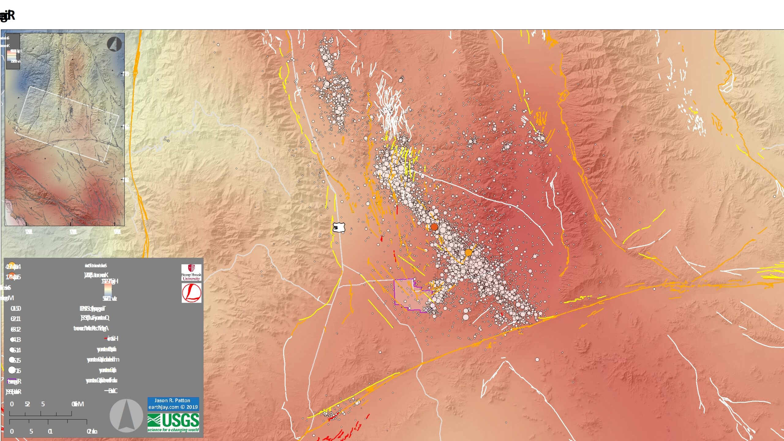
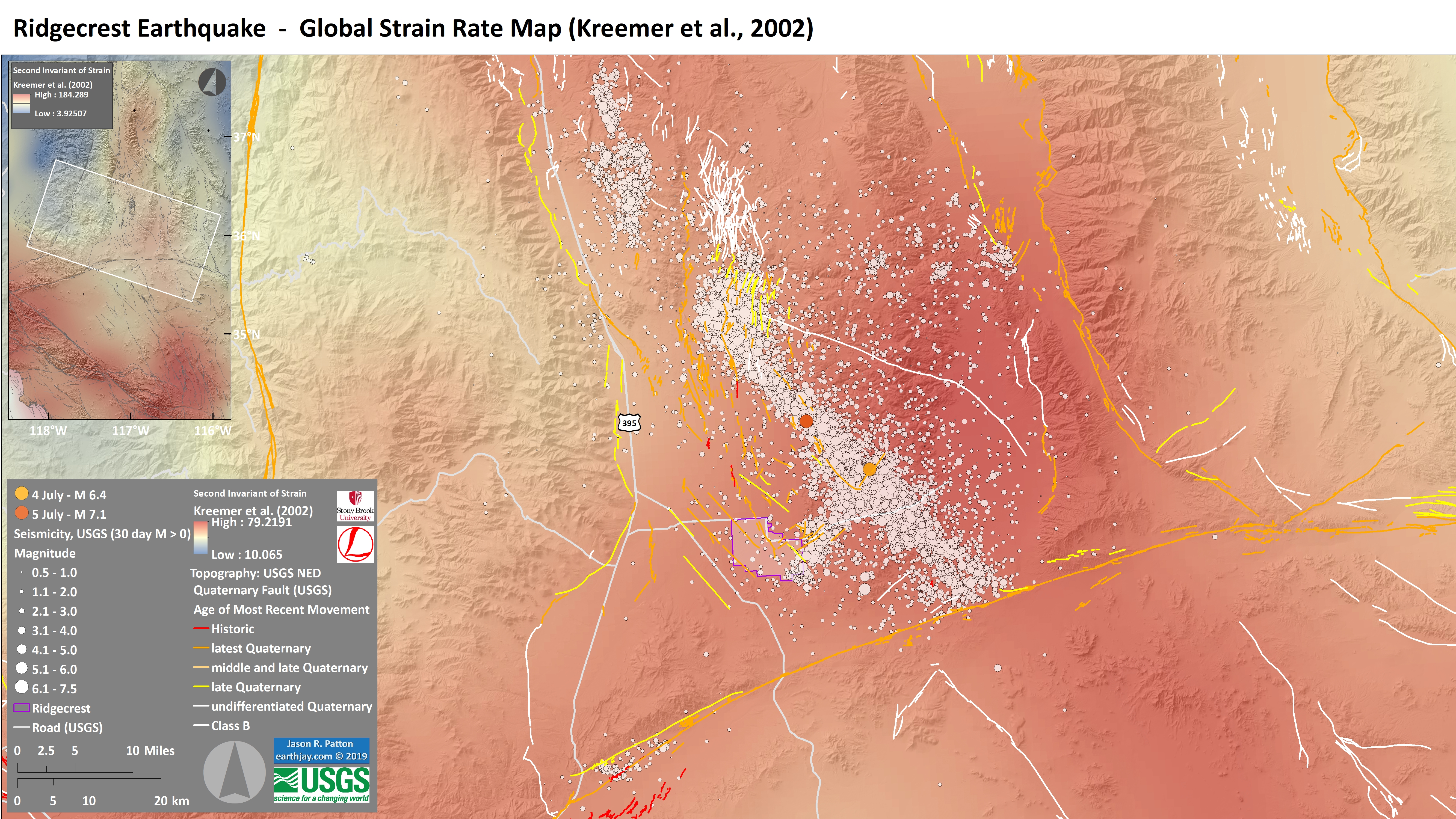
Global Strain Rate Map
- Strain is basically the change in shape or volume of a material through time. The Earth deforms with space and time in relation to geospatial variations in plate tectonic motions.
- Tectonic strain can be measured in a variety of methods. Most people are familiar with geodetic methods. Geodesy is the study of the motion of the Earth as measured at discrete locations (e.g. with GPS observations). One may use changes in position at GPS sites to measure how the Earth moves, so we can directly measure changes in shape this way.
- Geodetic data can be combined with geologic and seismicity data to evaluate tectonic strain at global, regional, and local scales.
- In 1998 the International Lithosphere Program started compiling a global dataset to support the construction of a Global Strain Rate Map (GSRM; Kreemer et al., 2000, 2002, 2003, 2014).
- The GSRM has been incorporated into the Global Earthquake Model of Seismic Hazard, v 2.1 presented online here.
- I present a map for the Ridgecrest Earthquake Sequence that uses an older version of the GSRM (v 1.2). The color ramp is based on the “second invariant” of strain. Warmer colors show regions of greater tectonic strain. Units are in 10
Geologic Map
- There are some larger scale geology maps for this region, but they cost money (Dibblee Foundation/AAPG). Needless to say, I don’t have the $50 to buy them right now. They are geotiffs, so would overlay nicely.
- The map below shows seismicity for the past month overlain upon the 1962 California Division of Mines and Geology 1:250,000 scale geologic map (Jennings et al., 1962). I prepared this on 21 July 2019 after georeferencing the map from the CGS website..

UNAVCO Response Page
- UNAVCO has event response pages where people post visualizations of data. Here is the Ridgecrest Earhquake Response Page.
OTA-measured GNSS static displacements from the real-time GNSS system (blue) compared to the seismically derived static displacements (pink).
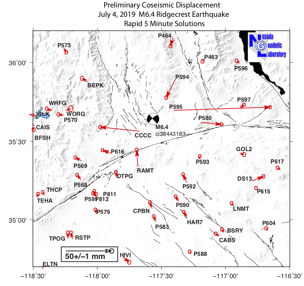
Preliminary coseismic horizontal vector displacements for the July 4, 2019 M 6.4 earthquake. The 5-minute sample rate time series were obtained using rapid orbits from the Jet Propulsion Laboratory.
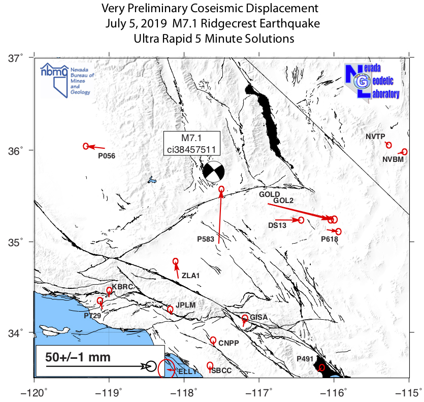
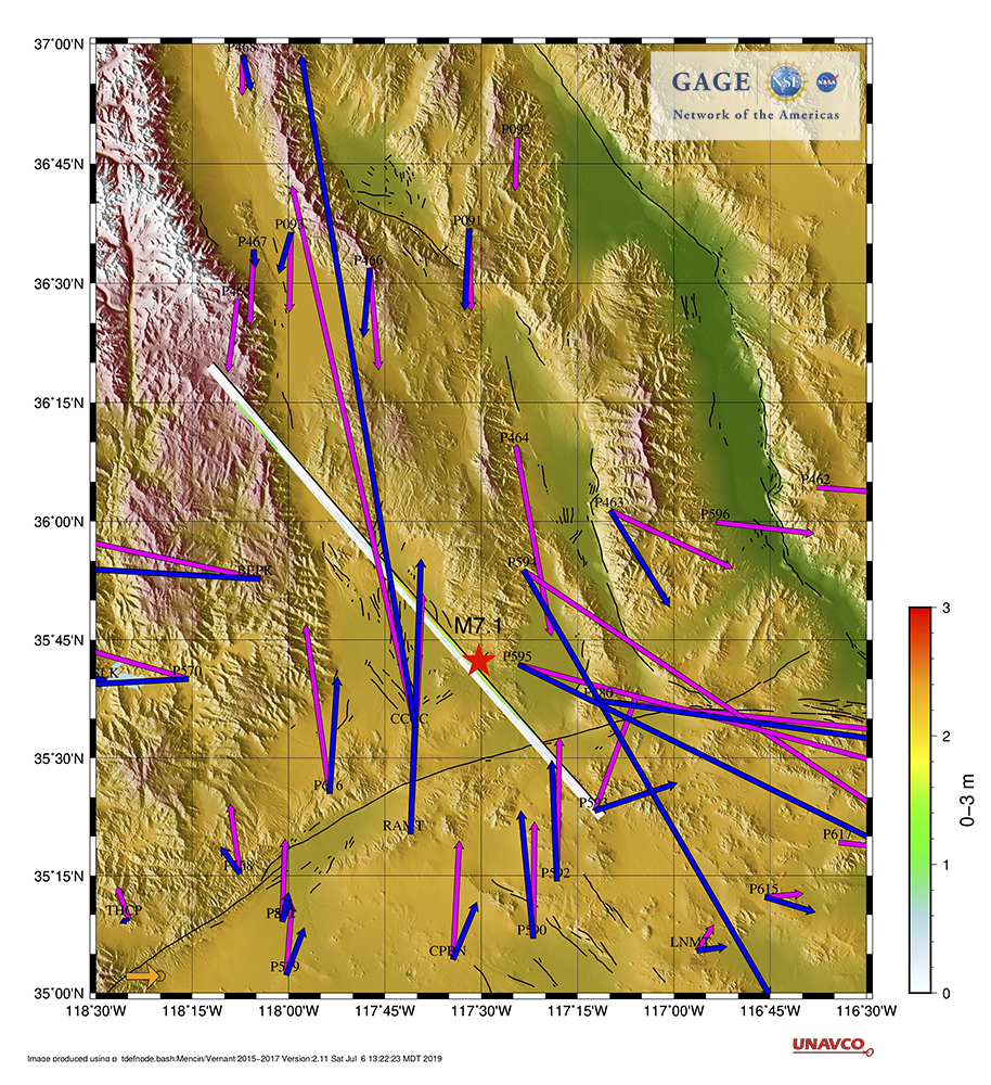
Ultra rapid analysis coseismic offsets calculated by the Nevada Geodetic Laboratory (NGL) for a subset of continuous GPS stations in the region of the July 6, 2019 M 7.1 earthquake.
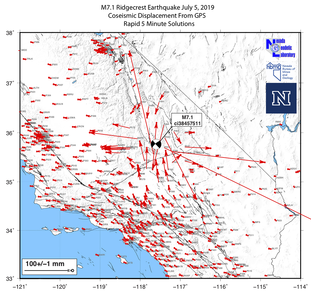
Rapid analysis coseismic offset pattern for the July 6, 2019 M 7.1 Ridgecrest earthquake, from the Nevada Geodetic Laboratory (NGL)
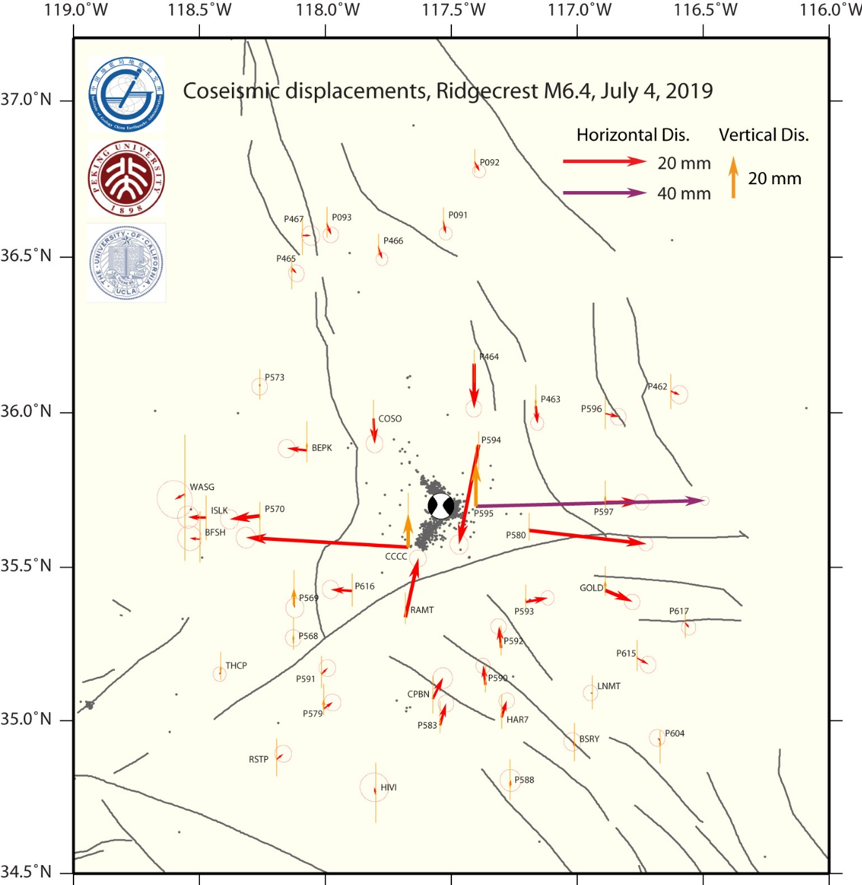
GPS derived coseismic displacements of Mw6.4 foreshock. Five days of GPS data spanning the foreshock and prior to the mainshock were processed to obtain the solution.
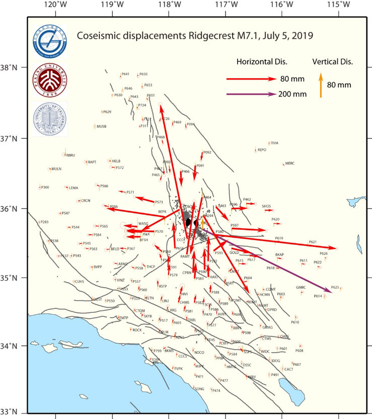
GPS derived coseismic displacements of Mw7.1 mainshock. Four days of GPS data spanning the mainshock and after the foreshock were processed to obtain the solution.
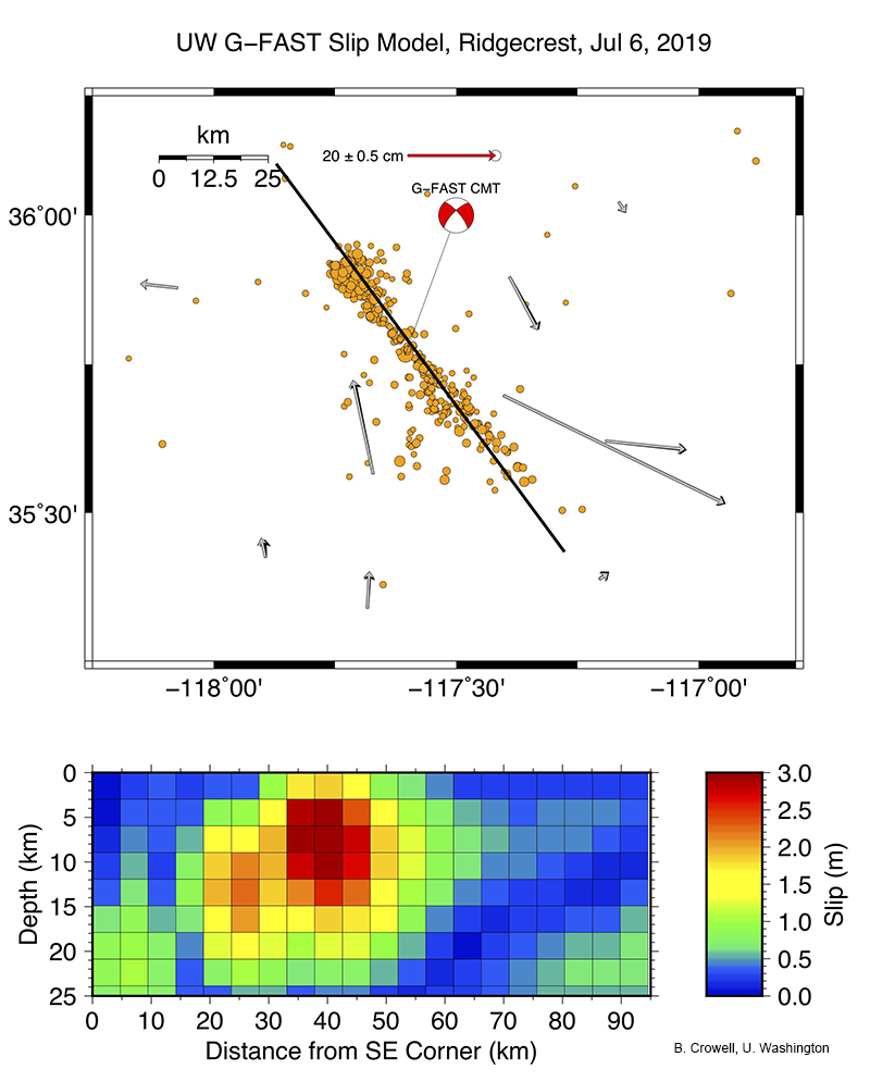
Preliminary slip results derived from geodetic and seismic data for the July 6, 2019 M 7.1 Ridgecrest earthquake, from the Pacfic Northwest Seismic Network. The slip model was run through G-FAST.
- Here is a video showing real time GPS displacement from 1Hz GPS/GNSS NOTA data analyzed by Christine Puskas.
Background Literature – Tectonics
- Here is a great overview map of the faults in the region from Oskin et al. (2008). Their paper is about their research to quantify the tectonic loading of faults in the Eastern California shear zone. Note that they use about 12 mm per year of Pacific-North America relative plate motion across this region.
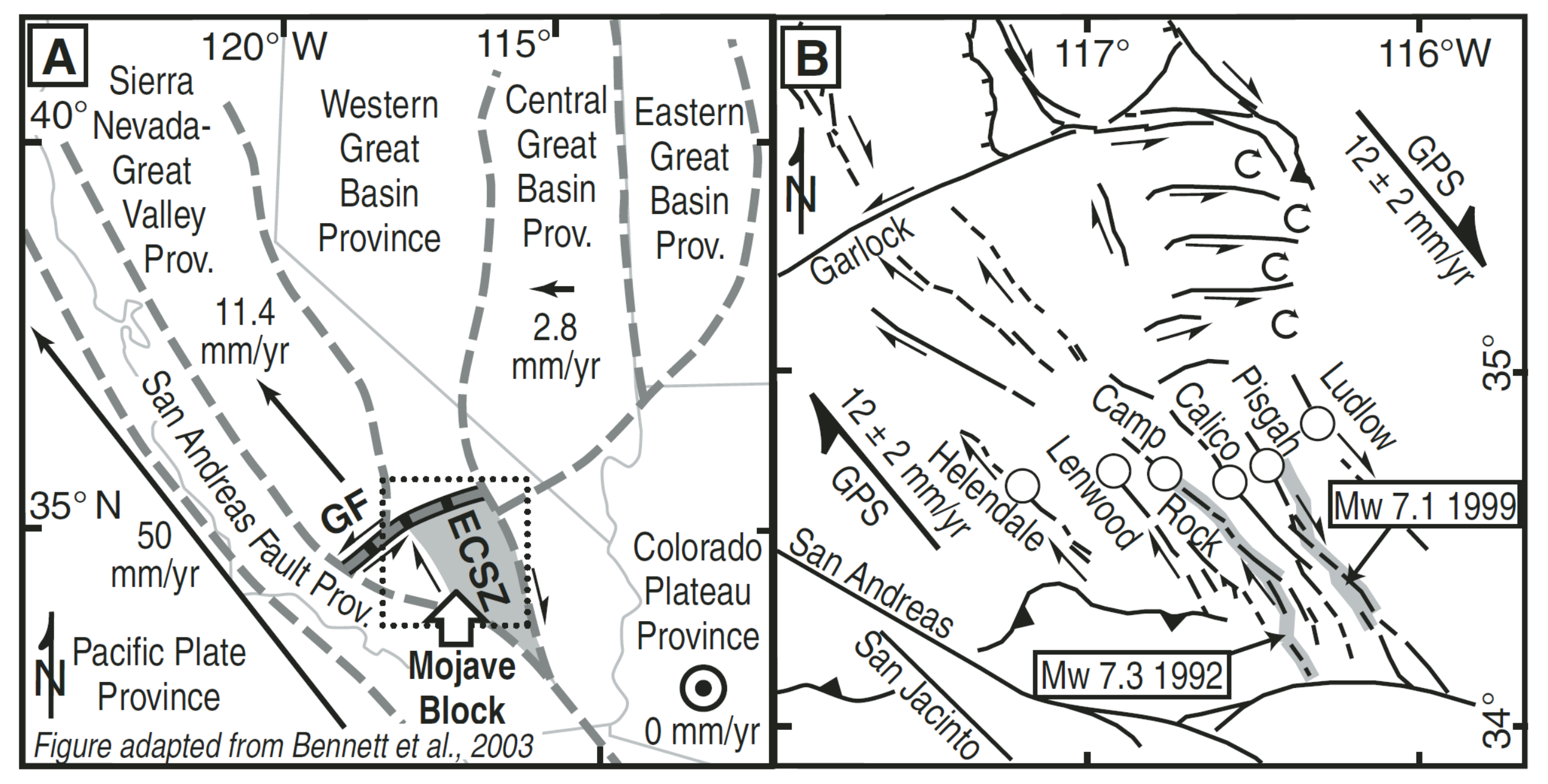
A: Index map of southwest North America showing geodetic provinces from Bennett et al. (2003) and location of Mojave block. Velocities of geodetically stable regions are shown relative to Colorado Plateau. ECSZ—eastern California shear zone in Mojave block. Shear zone continues northward into western Great Basin province. GF—Garlock fault. B: Index map of the Mojave block with active faults and locations of recent earthquake ruptures. Circles show localities of slip-rate measurements that sum to ≤6.2 ± 1.9 mm/yr across the ECSZ. GPS—global positioning system.
- Here is another good overview map, showing the faults for which Petersen and Wesnousky (1994) reviewed slip rates in that publication. They present an excellent review of all slip rate and paleoseismic investigations at the time that paper was published.
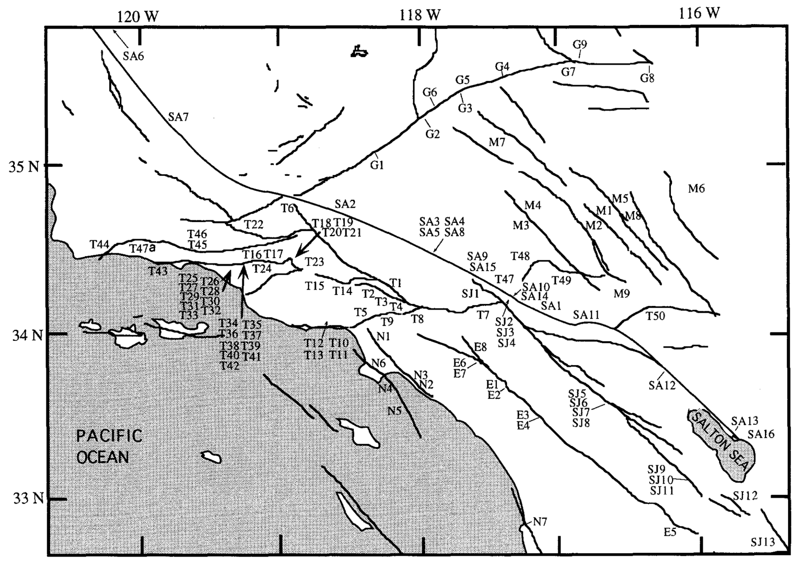
Map showing sites of slip rate studies in southern California for the San Andreas (SAI-14), San Jacinto (SJI-13), Elsinore-Whittier (El-8), Newport- Inglewood (N1-3), Palos Verdes (N4-6), Rose Canyon (N7), Transverse Ranges (T1-50), Mojave (MI-6), and Garlock (G1-9) faults.
- Oskin and Iriondo studied the Blackwater fault, the right-lateral strike-slip fault system that extends from the south into the region of the Ridgecrest Earthquake Sequence. The Blackwater fault is connected to the south with the Calico fault (a fault between the 1992 and 1999 earthquakes). This appears to be the major Eastern California Shear zone fault that extends towards the Airport Valley and Little Lake faults (which ruptured during the Ridgecrest Earthquake Sequence).
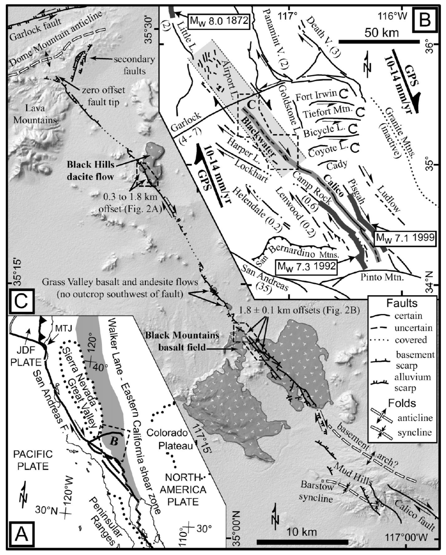
A: Index map of Pacific–North America plate boundary through southwest North America. Principal faults are shown as thick black lines. Tectonically stable areas are outlined by dotted lines. Walker Lane and Eastern California shear zone, shown as dark gray band encompassing network of active faults, together absorb 9%–23% of total plate boundary shear (Dixon et al., 2000; Dokka and Travis, 1990a). JDF—Juan de Fuca; MTJ— Mendocino triple junction. B: Index map of Eastern California shear zone showing fault slip rates (in parentheses, mm/yr) determined by paleoseismic studies (Klinger and Piety, 2000; Lee et al., 2001; McGill and Sieh, 1993; Rockwell et al., 2000; Zhang et al., 1990). Heavy dark gray lines outline historic earthquake ruptures (Beanland and Clark, 1994; Sieh et al., 1993; Treiman et al., 2002). Heavy, medium gray band highlights Blackwater–Calico fault system. Light gray band surrounding Blackwater fault and passing north of Garlock fault is zone of localized 1.2 6 0.5 mm/yr strain accumulation documented by radar interferometry (Peltzer et al., 2001). C: Neotectonic map of Blackwater fault, showing type and orientation of fault line scarps with ticks on downthrown side. Dark patterned areas are lava flows cut by Blackwater fault (Dibblee, 1968, 1967; Smith, 1964)
- Peltzer et al. (2001) evaluate the amount of tectonic strain that has accumulated over time (see geodesy section to learn more about strain). First I present their tectonic map.
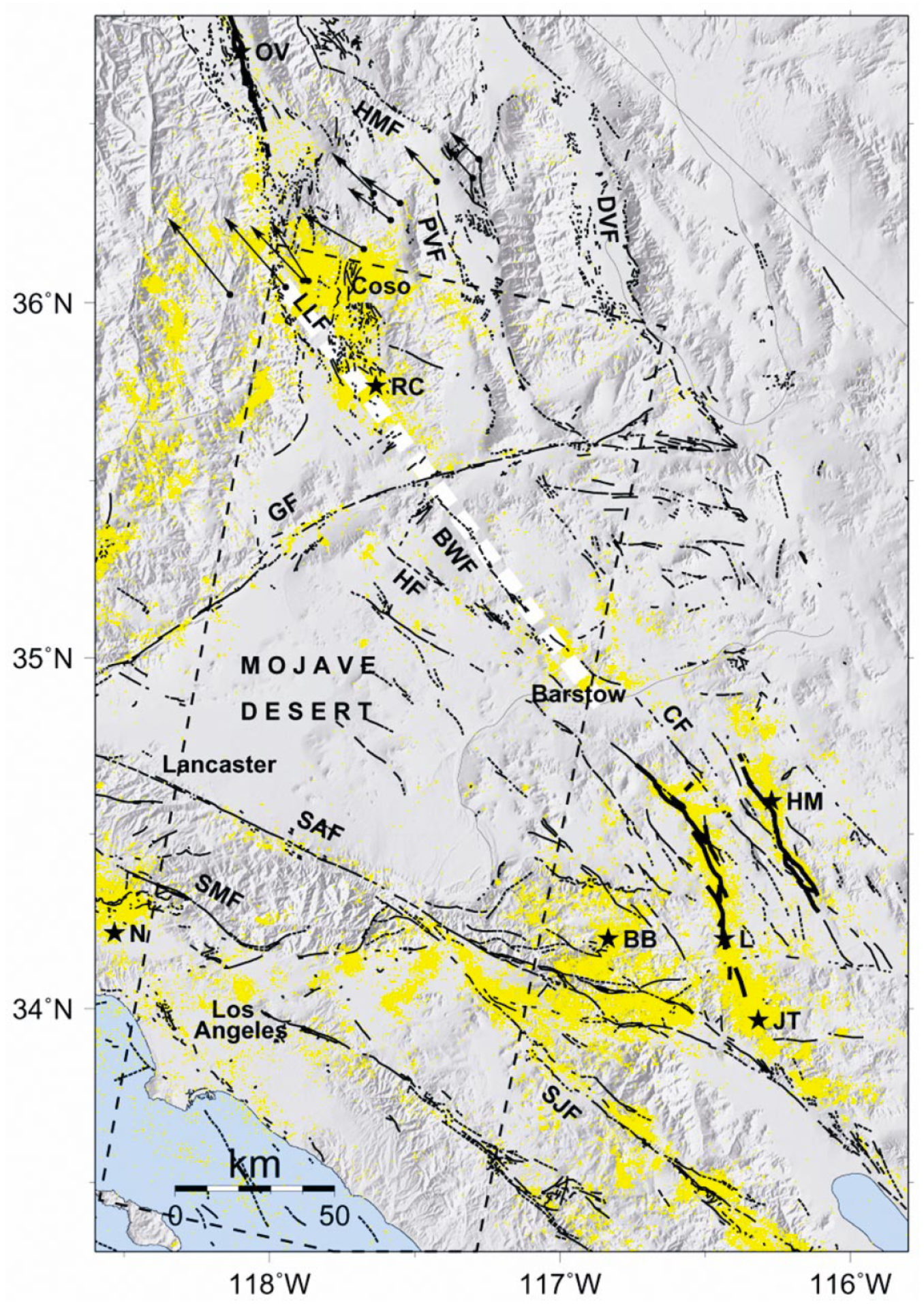
Tectonic map of southern California. Solid lines are active faults (Jennings, 1975). Yellow dots are relocated earthquakes between 1981 and 2000 (Hauksson, 2000). Dashed-line box is area covered by Earth Resource Satellite (ERS) data used in this study. White dashed line shows location of concentrated shear observed in synthetic aperture radar (SAR) data. Black stars indicate epicenters of recent earthquakes: OV—1872 Owens Valley, JT—1992 Joshua Tree, L—1992 Landers, BB—1992 Big Bear, N—1994 Northridge, RC—1994 and 1995 Ridgecrest, HM—1999 Hector Mine. Heavy solid lines depict surface ruptures of Landers (Sieh et al., 1993), Hector Mine (U.S. Geological Survey and California Division of Mines and
Geology, 2000; Peltzer et al., 2001), and Owens Valley (Beanland and Clark, 1994; only southern half of rupture is shown) earthquakes. Black dots and arrows show locations and observed velocities of 11 stations of Yucca GPS array (Gan et al., 2000).
* Faults are listed in the paper
- Guest et al. (2003) used geologic mapping and geochronologic data (ages of geologic units) to constrain a tectonic model. They suggest that some of the faults in the region developed as a result of tectonic blocks rotating about a vertical axis. First we see their geologic map.
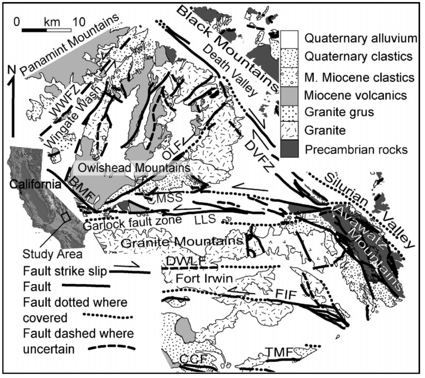
Segment of Trona sheet geologic map showing Owlshead block, southern Death Valley, and Northeast Mojave block. WWFZ— Wingate Wash fault zone, BMF—Brown Mountain fault, OLF—Owl Lake fault, DVFZ—Death Valley fault zone, MSS—Mule Springs strand, LLS—Leach Lake strand, DWLF—Drink Water Lake fault, FIF—Fort Irwin fault, CCF—Coyote Canyon fault, TMF—Tiefort
Mountain fault.
- Here is the Guest et al. (2003) map showing their interpretation of how these faults developed over time.

In this model the Owlshead and southern Panamint blocks are hypothesized to have undergone sinistral transtension in response to a clockwise rotation of their southern confining boundary (Garlock fault zone).
RTR—Radio Tower Range, SOM—Southern Owlshead Mountains, WWFZ—WingateWash fault zone, BMF—Brown Mountain fault, OLF—Owl Lake fault, GF—Garlock fault, MSS—Mule Springs strand, LLZ—Leach Lake fault zone, SDVFZ—Southern Death Valley fault zone.
Background Literature – Geodesy
- Gan et al. (2003) present a summary of geodetic data where they show that the Owens Valley, Little Lake, and Helendale faults form the generalized western boundary of the Eastern California shear zone (there are additional right-lateral faults to the west however).
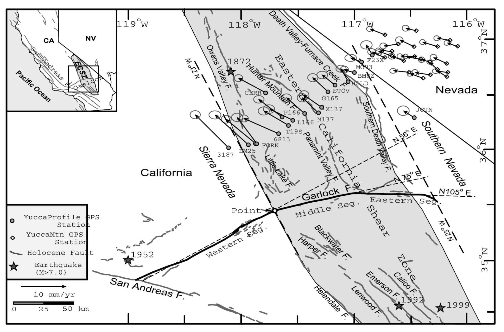
Map showing the location of the ECSZ, the GPS arrays, the station velocities (relative to the fixed North America), and the principal faults in southern California (from Jennings [1992]). The thick dashed lines directed N23°W show the boundaries of the assumed parallel-sided ECSZ. The thin dashed lines extended from the segments of the Garlock fault show the trends of the segments.
- One of the challenges with interpreting geodetic data is comparing earthquake fault slip rates inferred from geodetic methods with rates calculated using geologic data (either from long term offsets of bedrock, or from more recent rates using fault trenches).
- Chuang and Johnson (2011) present their comparisons of GPS slip rates with geologic rates.
- Blue = geologic rate
- Black = geodetic rate
- Magenta = block model rate from their analyses
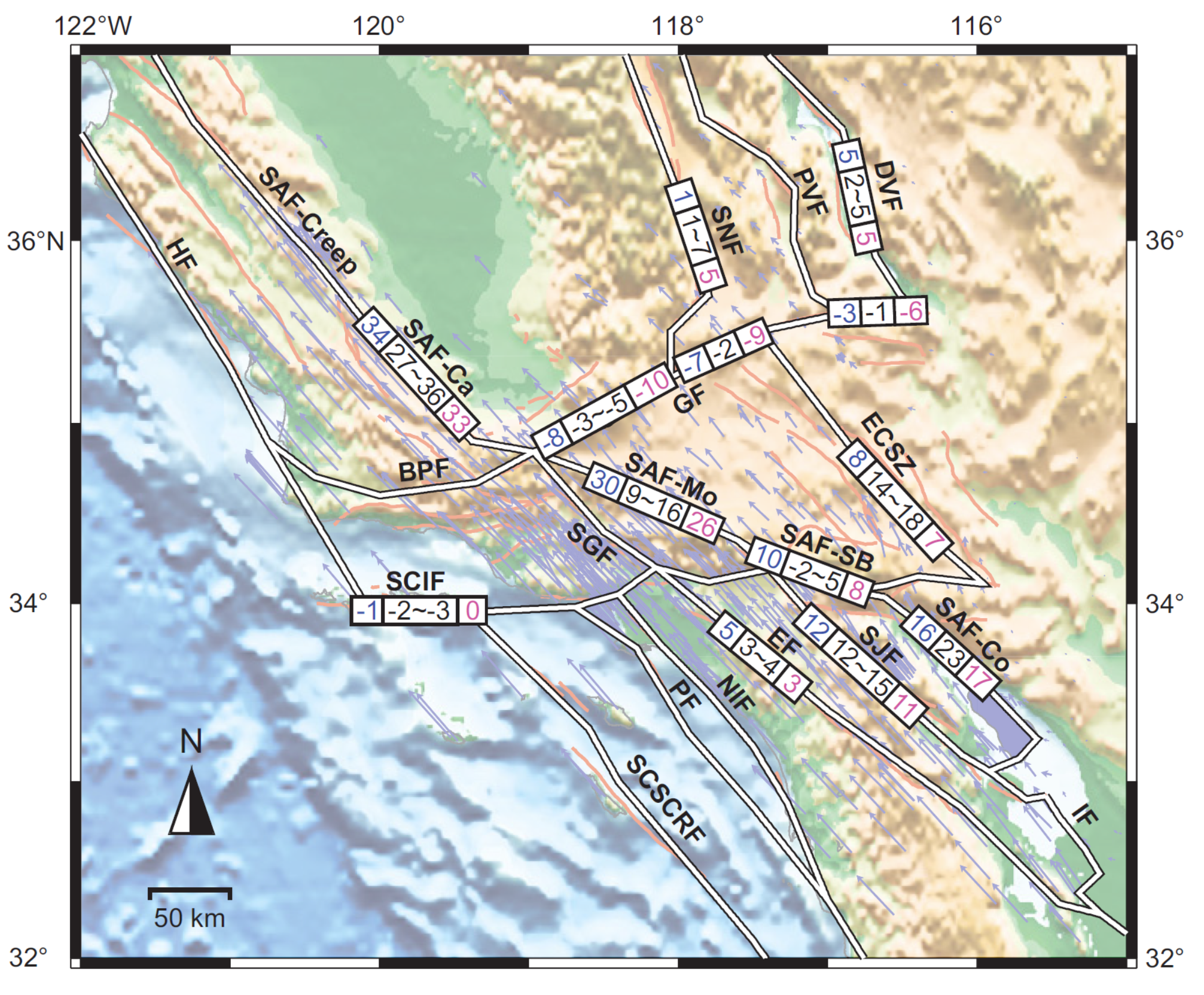
Comparison of geologic fault slip rates (blue, mm/yr) used in model, range of estimates from elastic block models (black) of Becker et al. (2005) and Meade and Hager (2005), and estimates from our block model (magenta) along major faults. Negative is left lateral. Light red lines are surface fault traces, and white thick lines are model blocks. Blue arrows are Southern California Earthquake Center (SCEC) crustal motion map 3 (Shen et al., 2003) velocities with respect to stable North America.
*See their paper for fault abbreviations.
- Here is an interesting figure showing their (Chuang and Johnson, 2011) estimate of the relative position in the earthquake cycle for these faults. This is based on published recurrence intervals for these faults (the average time between earthquakes given paleoseismic investigation data).
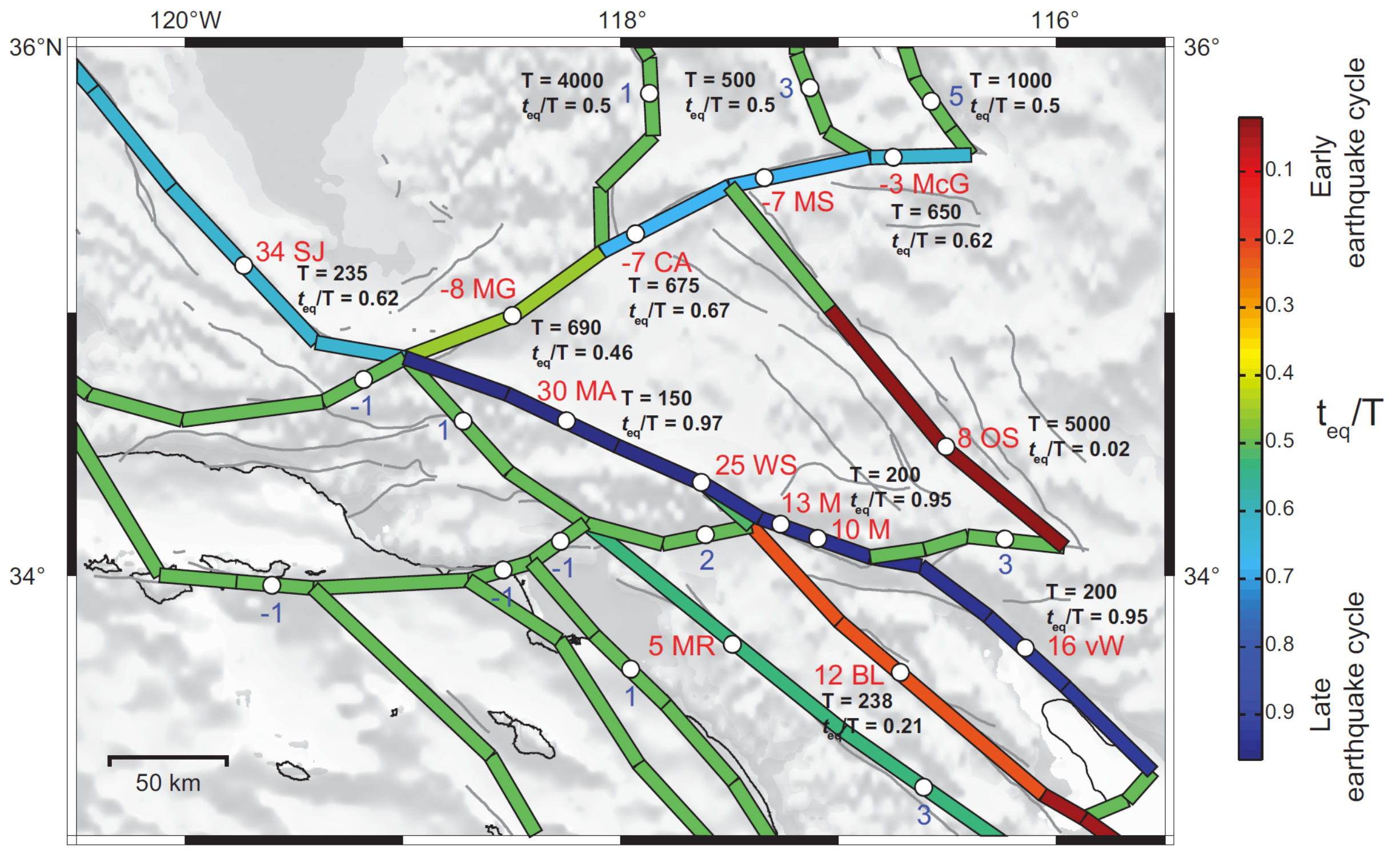
Summary of assumed geologic rates, recurrence interval (T), and time since last earthquake (teq) in Southern California. (For further discussion of sources of T and teq, see footnote 1). Blue numbers are expert opinion slip rates from Working Group on California Earthquake Probabilities (2008) and red numbers are rates from other paleoseismology data.
Color of rupture segment represents ratio of time since last earthquake and recurrence interval. Hot (red) colors show segments are in early earthquake cycle, and cold (blue) colors show late earthquake cycle.
- This is the summary of the Chuang and Johnson (2011) slip rate comparison.
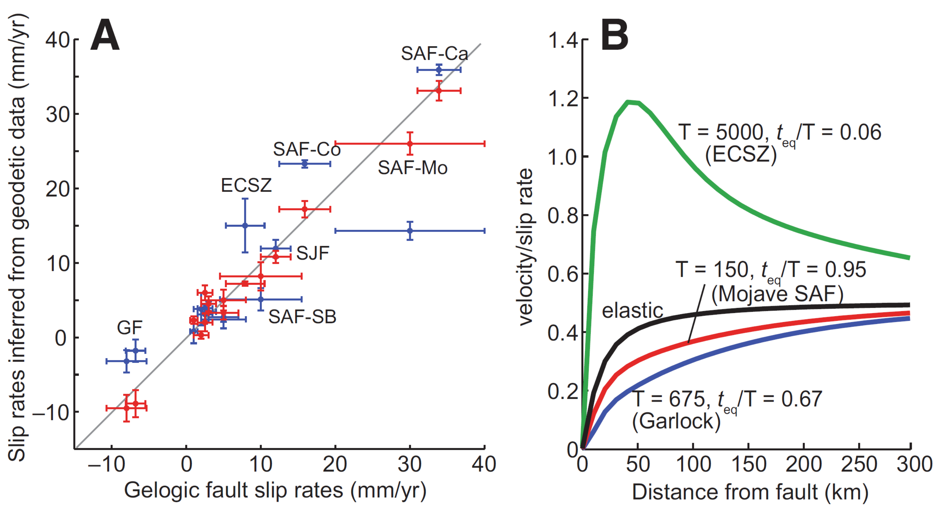
A: Geologic fault slip rates versus slip rates inferred from geodetic data. Geologic rates are summarized in Table DR1 (see footnote 1). Blue bars are slip rate comparisons from Meade and Hager (2005) and red bars are from this study. B: Normalized velocity across Garlock fault (blue), Mojave segment of San Andreas fault (red), and eastern California shear zone (ECSZ, green) from our cycle model. Black line is normalized velocity derived from elastic model.
- Here is an earlier analysis comparing geodetic rates with geologic rates (Dixon et al., 2003). First we see a map showing the faults from which the fault comparisons are shown.
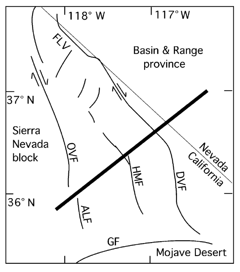
Sketch map of study area, modified from Dixon et al. (1995). Bar marks approximate location of Global Positioning System transect (Gan et al., 2000). GF— Garlock fault. Labeled faults of Eastern California shear zone: ALF— Airport Lake fault zone; OVF—Owens Valley fault zone; HMF—Hunter Mountain–Panamint Valley fault zone; DVF— Death Valley–Furnace
Creek fault zone; FLV— Fish Lake Valley fault zone.
- Here is the east west profile from Dixon et al. (2003). The horizontal axis is distance and the vertical axis is the rate that each site moves in mm per year. Their fault modeling is represented by the dark black line.
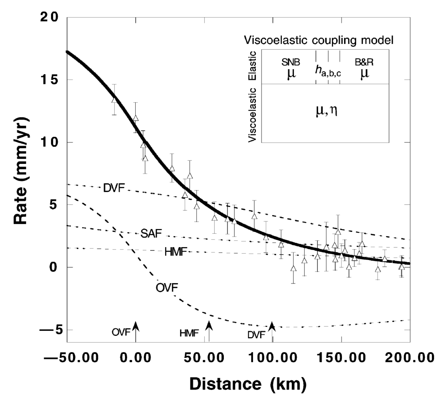
Global Positioning System velocity (triangles) and one standard error (bars) from Gan et al. (2000) compared to prediction of viscoelastic coupling model (heavy solid line), representing summed velocity contributions from four parallel faults (light dashed lines). SAF—San Andreas fault; DVF—Death Valley–Furnace Creek fault zone; HMF—Hunter Mountain–Panamint Valley fault zone; OVF—Owens Valley fault zone. Inset shows model rheology for Eastern California shear zone. SNB—Sierra Nevada block;B&R— Basin and Range Province; h is fault depth (depth of elastic layer) for three faults (a, b, or c), m is rigidity, h is viscosity. Arrows mark location of major shear-zone faults.
- Peltzer et al. (2001) use synthetic aperture radar interferometry (see my second update report for more on InSAR anslysis) to measure tectonic deformation that accumulated between 1992-2000.
- Alos, check out a more recent analysis using InSAR in CA here.
- The Coso Geothermal Field is the rainbow area in the northernmost part of the map. Indian Wells Valley is the green area to the south of the Coso Field. This is an area of elevated strain. The Garlock fault is the ~east-west black line in the center of the white inset box.
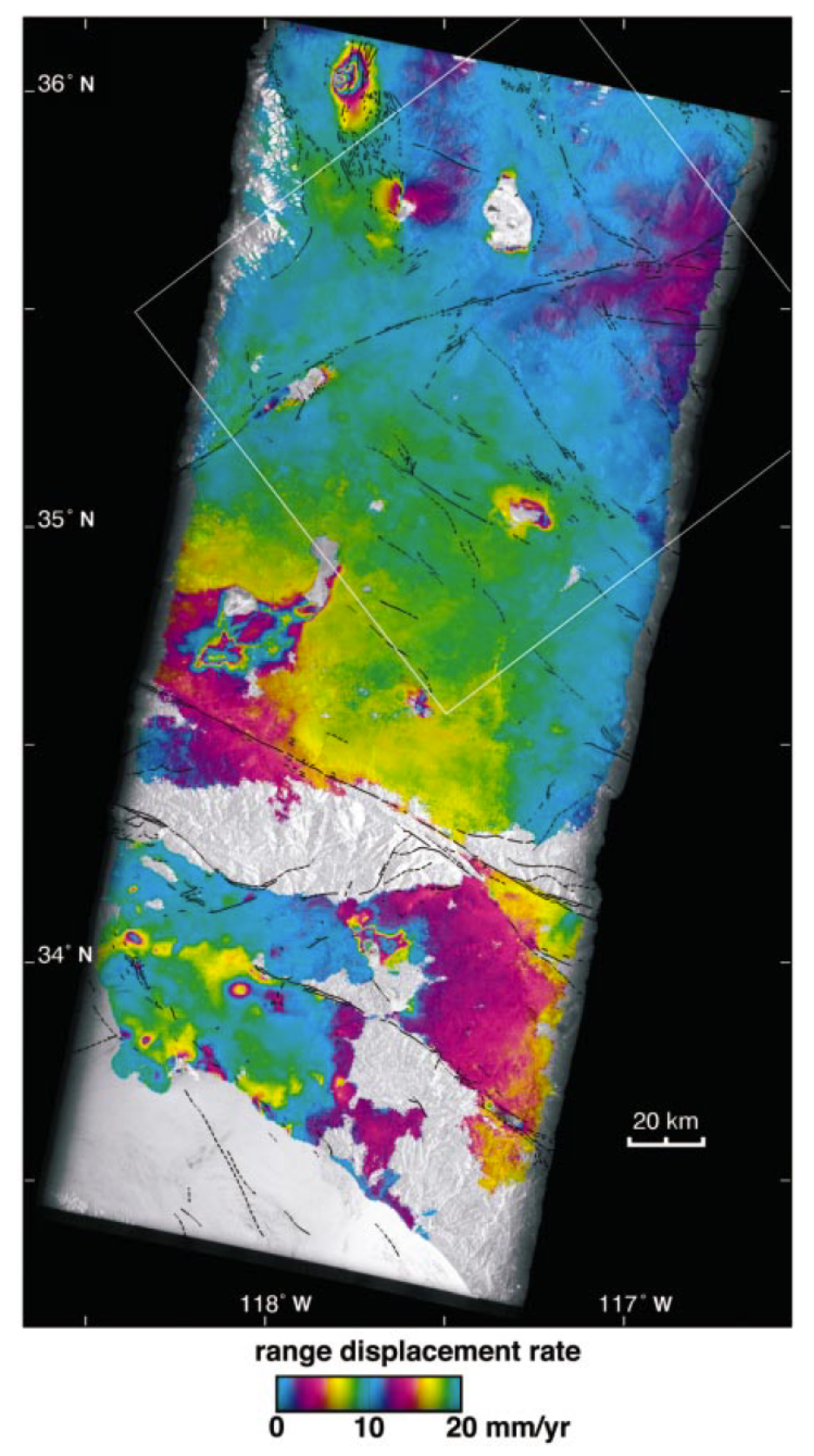
Surface velocity map obtained by averaging 25 interferograms of Los Angeles–Mojave region. One color cycle depicts 10 mm/yr of surface displacement along radar line of sight (at lat N348; ERS [Earth Resource Satellite] descending track trends S13.68W, radar looking westward at 238 off vertical incidence angle in middle of imaged swath). Gray areas are zones of low phase coherence that have been masked in processing. Black lines are active faults (Jennings, 1975). White box indicates subset of synthetic aperture radar (SAR) data that was used for profile in Figure 4. Note conspicuous shear strain along San Andreas fault and shear zone parallel to Blackwater–Little Lake fault system. Large deformation signal in northwest corner of frame is ground subsidence related to Coso volcanic and geothermal field (Fig. 1). Surface displacement associated with 1994 and 1995 Ridgecrest earthquakes is visible south of Coso area. Other patterns of surface deformation include ground subsidence due to groundwater withdrawal in Los Angeles and Lancaster areas (Fig. 1) and to seasonal change of water table level around dry lakes.
- Peltzer et al. (2001) plot observations from their radar data showing relative plate motion associated with dislocation along the Blackwater-Little Lake fault system.
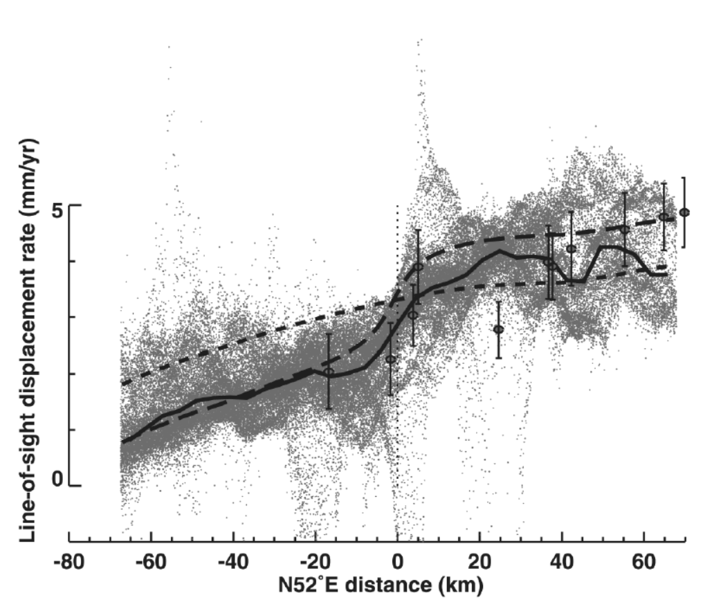
Profiles of observed and modeled line-of-sight displacement projected on vertical plane perpendicular to shear zone. Gray dots are individual data points for all radar-image pixels included in box shown in Figure 3. Solid line shows 2 km running mean of observed displacement along profile length. Note that apparent standard deviation of projected data relative to average profile reflects in part displacement gradient parallel to fault strike and not only error in data. Groups of dots that deviate from dense part of profile are due to ground subsidence near lake shores and to surface displacement associated with Ridgecrest earthquakes (Figs. 1, 3). Short-dash line is profile predicted by long-term velocity model used to estimate interferometric baseline (Shen et al., 1996). Long-dash line is profile predicted by velocity model, including additional buried dislocation along Blackwater–Little Lake fault system. Parameters of added fault are given in text. Black dots and error bars (2s) are line-of-sight projections of horizontal velocities observed by GPS at stations of Yucca transect (Gan et al., 2000).
Background Literature – Little Lake fault
- Amos et al. (2013) presented an analysis of “tectonic, geomorphic, and volcanic” features to derive a slip rate for the Little Lake fault near Little Lake, California. This is just northwest of the 2019 Ridgecrest Earthquake Sequence. Here is their tectonic map.
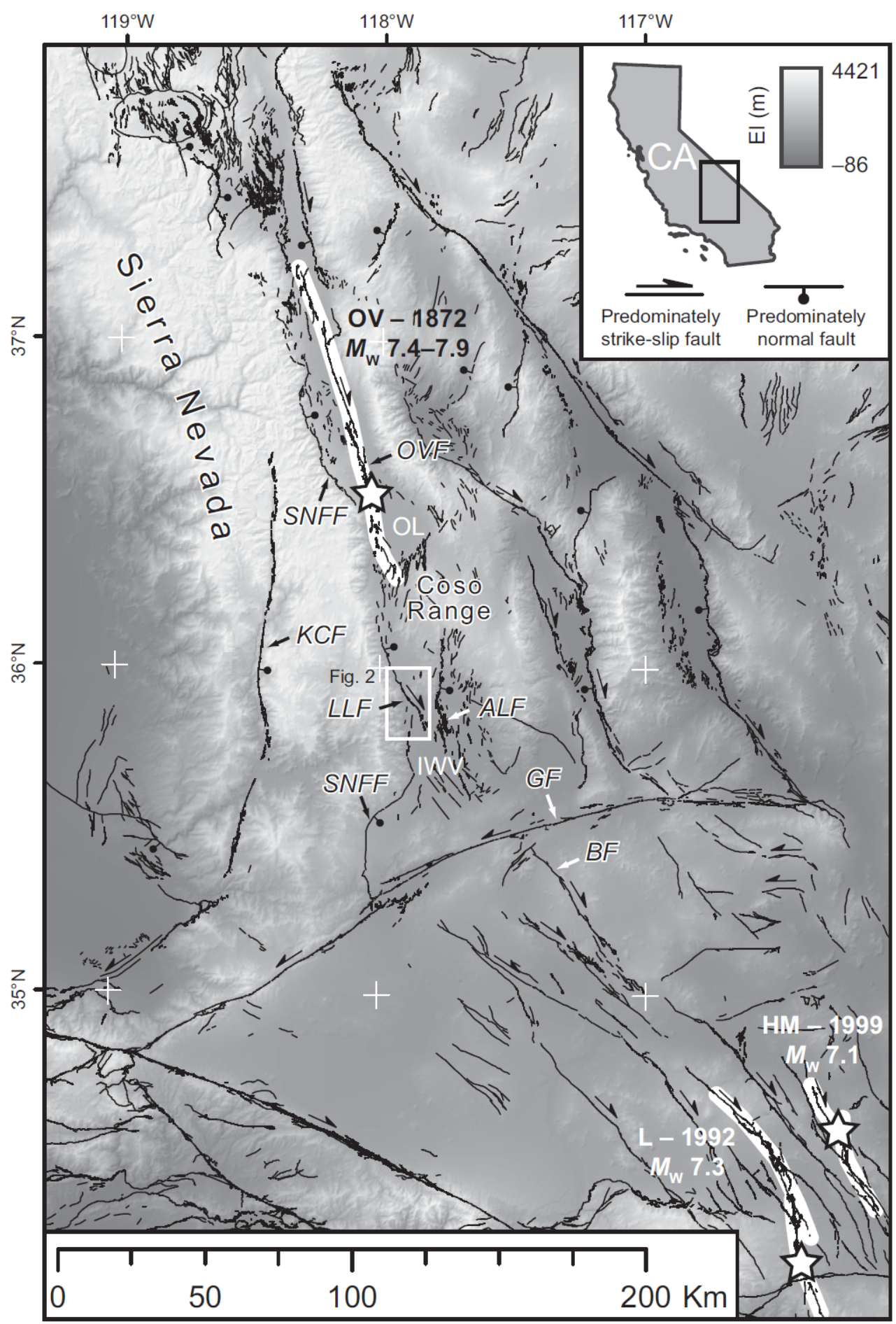
Overview of active faults and regional topography of the Eastern California shear zone (ECSZ) and southern Walker Lane belt. Labeled faults are abbreviated as follows: ALF—Airport Lake fault, BF—Blackwater fault, GF—Garlock fault, KCF—Kern Canyon fault, LLF—Little Lake fault, OVF—Owens Valley fault, SNFF—Sierra Nevada frontal fault. OL—Owens Lake, IWV—Indian Wells Valley. Major historical earthquake surface ruptures in the Eastern California shear zone and Walker Lane belt are outlined in white, with stars denoting epicentral locations: OV—1872 Owens Valley, L—Landers 1992, HM—1999 Hector Mine. Active fault traces are taken from the U.S. Geological Survey Quaternary fault and fold database, with the exception of the Kern Canyon fault, taken from Brossy et al. (2012).
- Here is a geologic map from Amos et al. (2013) that shows the mapped faults and topographic controls of river drainage for the area.
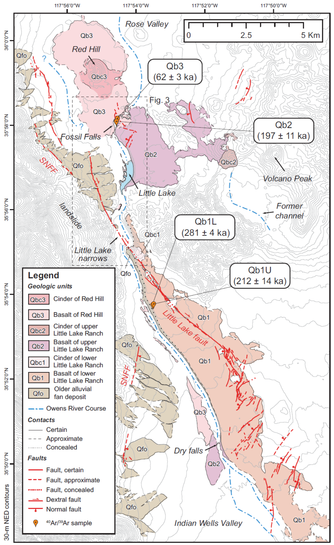
Simplified geologic map of the Little Lake fault, highlighting Quaternary volcanic and alluvial deposits bearing on the Pleistocene drainage of Owens River through the Little Lake area. Map units are named and modified from Duffield and Bacon (1981). The 30 m elevation contours are taken from the National Elevation Database (NED). The 40Ar/39Ar dates are labeled as in Table 1. SNFF—Sierra Nevada frontal fault.
- Here is a figure that shows the topography at the Amos et al. (2003) slip rate site along the Owens River. They measured topographic profiles of the ground surface across topographic landforms. These profiles were taken along the thin white lines on the map on the left.
- On the right are the profiles from the western (B) and the eastern (C) profiles are shown on the right. They use these offset features, and the distance that they are offset, to calculate the slip rate here.
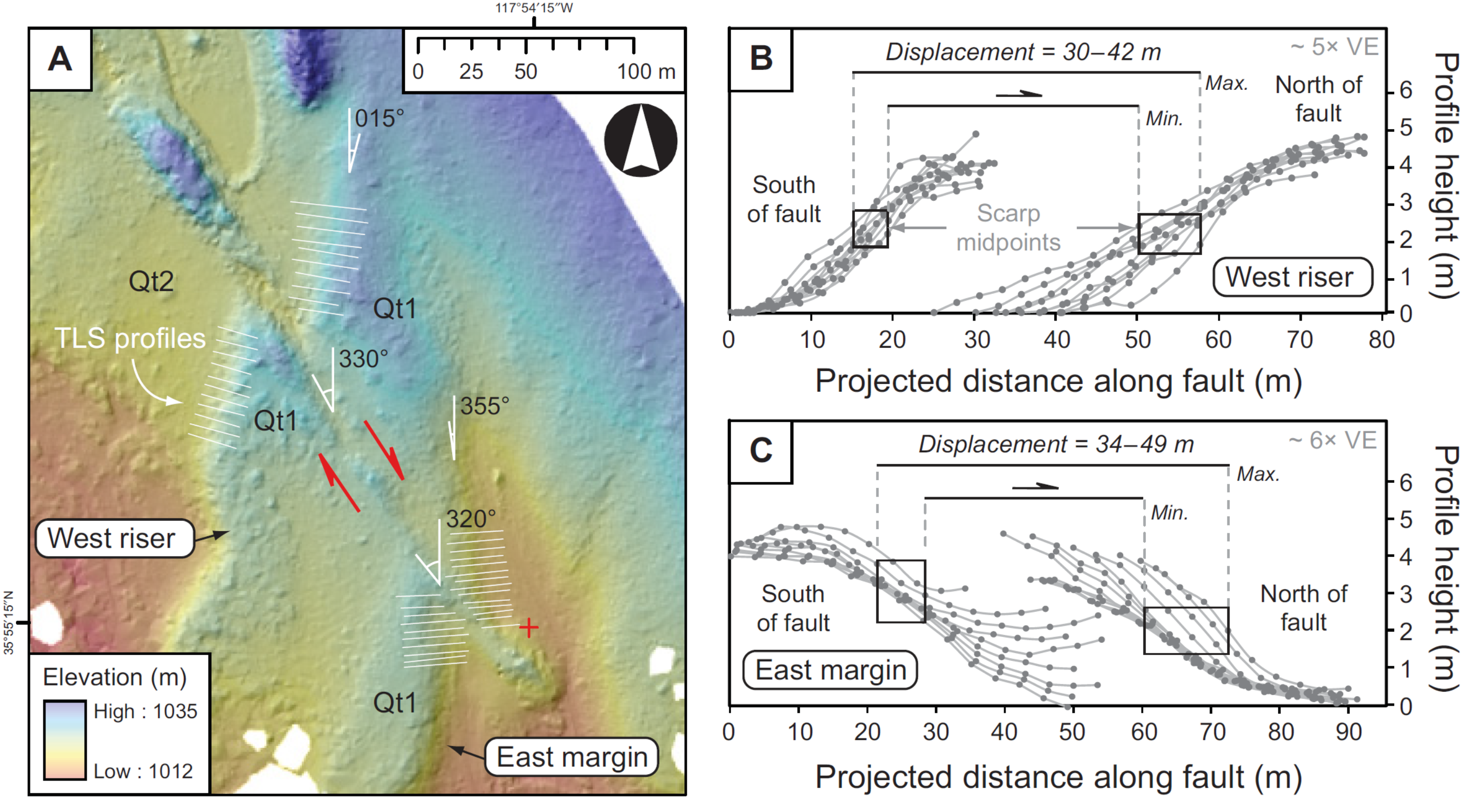
(A) 50 cm digital elevation model derived from terrestrial laser scanning (TLS) of displaced terrace risers in Little Lake narrows. (B–C) Stacked topographic profiles along the western and eastern edges of the Qt1 surface, respectively, used to reconstruct the total dextral offset of the Qt1-Qt2 terrace riser. Individual profiles were extracted perpendicular to the average riser orientation and were then projected onto a plane parallel to the local fault strike. Profile locations for each margin are shown in A. VE—vertical exaggeration.
- This is one of the coolest figures I found during my literature review. Amos et al. (2013) back calculate what the ground surface would look like if back in time, before the fault started to offset the topography here.
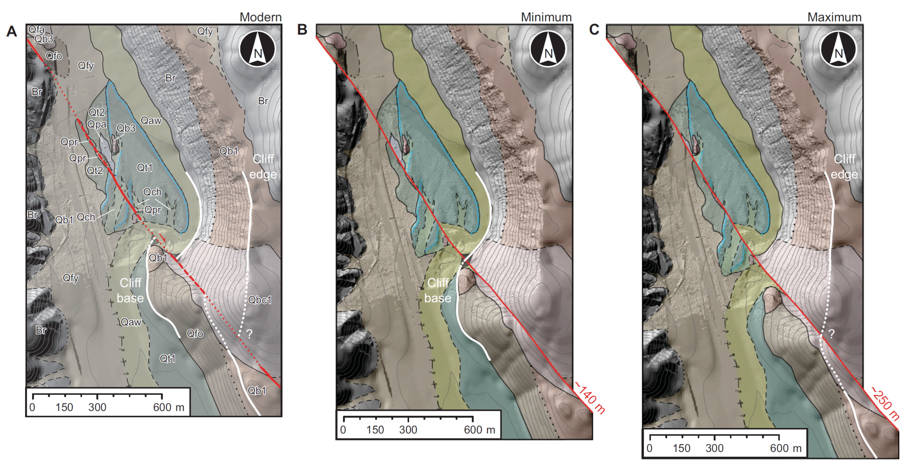
Geometric reconstruction of (A) the modern geomorphic configuration of the upper Little Lake narrows indicates between ~140 and 250 m of dextral offset for the base (B) and upper edge (C) of the eastern canyon wall. Geologic units are labeled as in Figure 3. The base image includes a hillshade image from our terrestrial laser scanning (TLS) survey, as
well as 10 m contours overlain on a National Elevation Database (NED) hillshade map. The map location is shown by the boxed area in Figure 3. Geologic units are labeled as in Figures 2 and 3.
- This is a cool figure, but not as cool as the above map. Amos et al. (2013) plot their slip rate estimates compared to published rates. First they show their observations of displacement relative to the age of the offset topographic landform. Then they plot slip rate estimates in the same manner.

(A) Compiled dextral displacements and (B) corresponding fault-slip rates as a function of age for the Little Lake, Blackwater, and Garlock faults. Linear regressions in A indicate constant slip rates through time. Geologic slip rate estimates in B are for time intervals since the respective age measurements. Geodetic measurements represent
interseismic deformation measured from interferometric synthetic aperture radar (InSAR) and global positioning system (GPS). […]
Background Literature – Garlock fault
- Astiz and Allen (1983) studied the seismicity of southern California and looked specifically at earthquake mechanisms associated with the Garlock fault. First we see their seismicity map for the region, then we zoom into the Garlock fault.
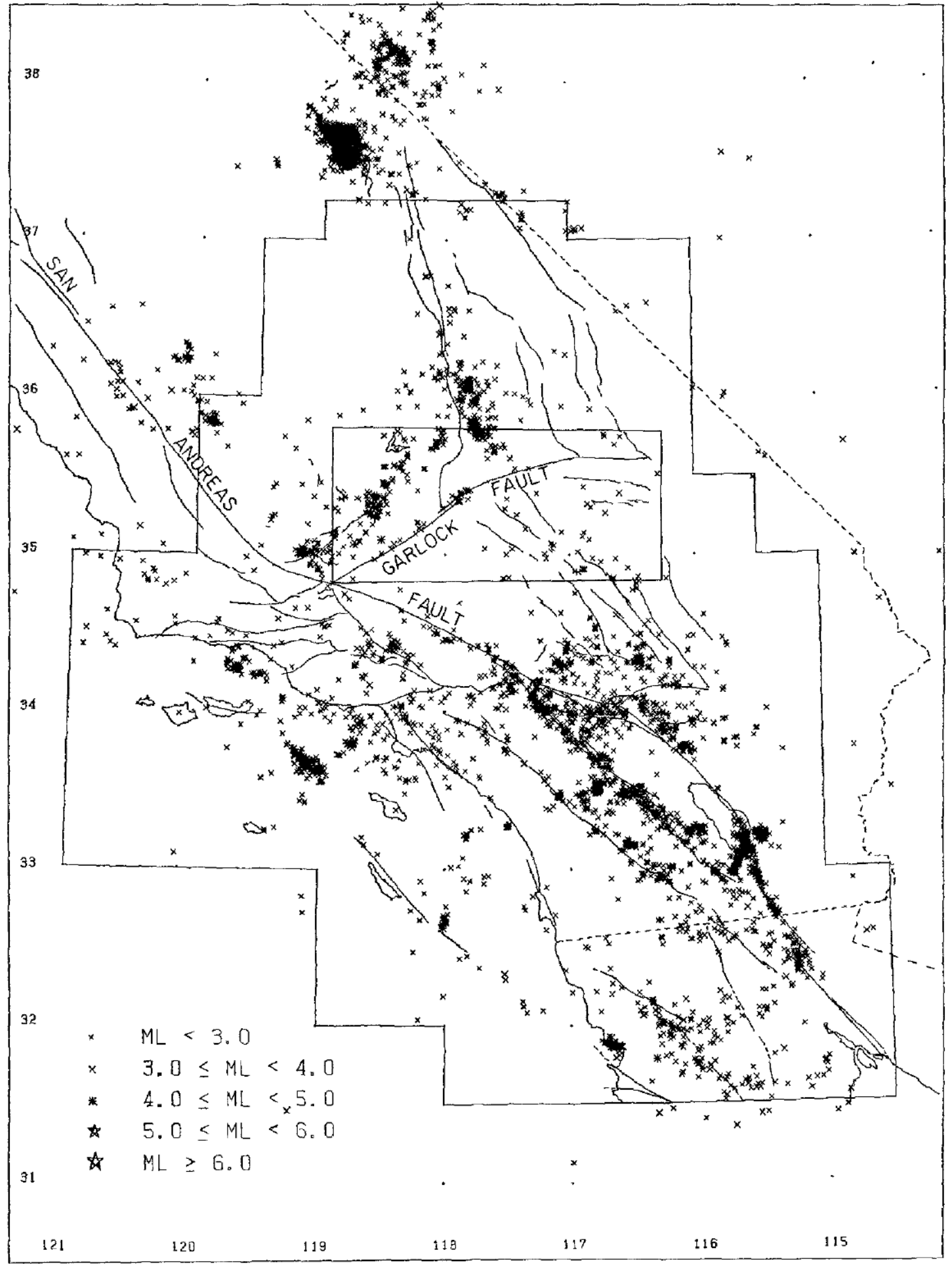
Southern California seismiclty during 1981 from Caltech-USGS catalog. The outer border corresponds to the limits of the southern California array. The inner frame is the limit of Figures 2 and 6. Notice the cluster of earthquakes along the Garlock fault trace and the smaller activity w~th respect to many other faults in southern California.
- Astiz and Allen (1983) plot the earthquake locations that they relocated for their analyses. This map shows a detailed map of the faults in the area..
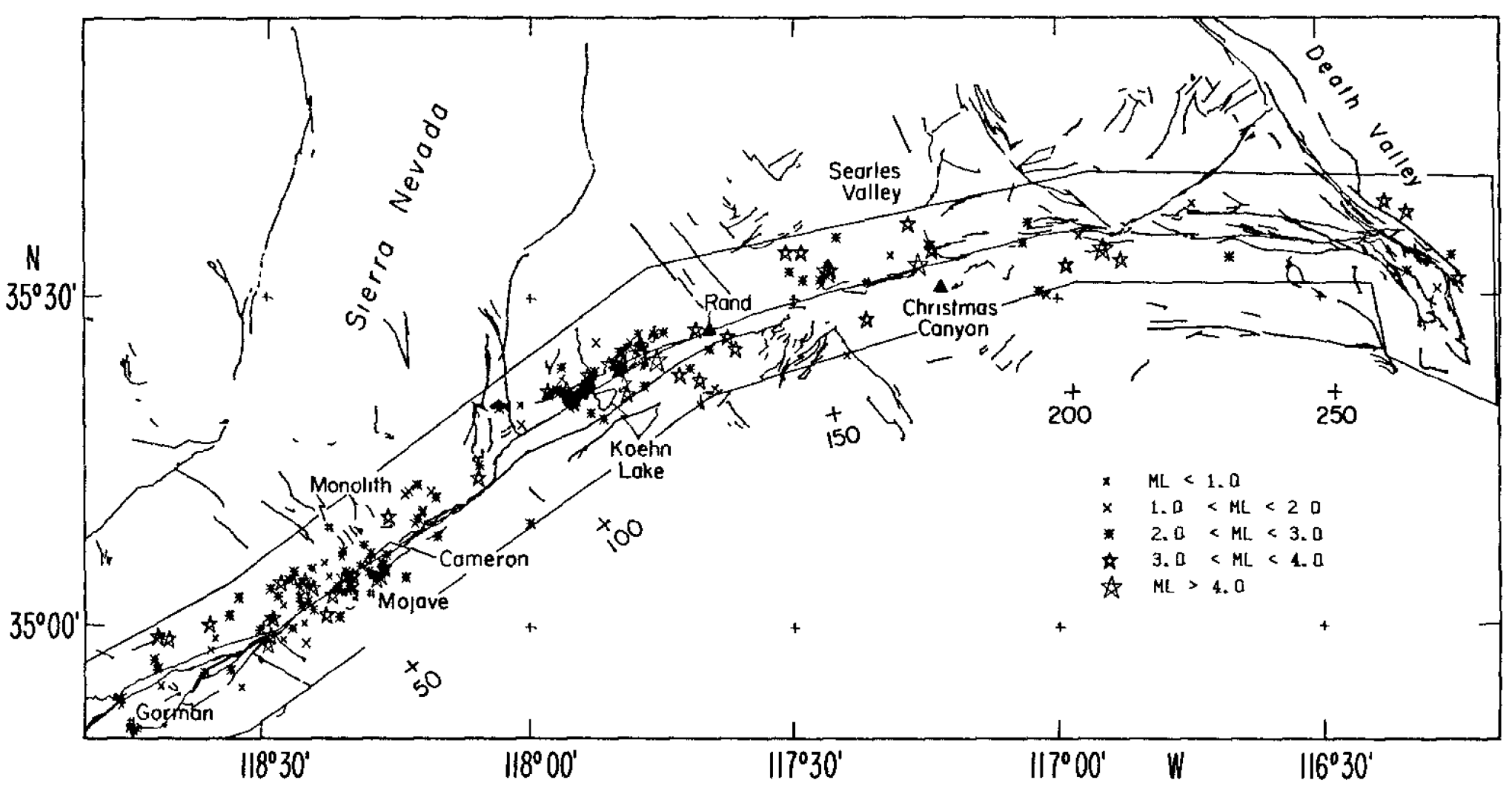
Earthquake relocations from 1932 to 1981 in the Garlock fault zone. The light line corresponds to the 25-km-wide zone around the fault from which the earthquakes were taken from the catalog. The numbers m the figure corresponds to kilometers along the fault northeast from Gorman quarry (vertical axes in Figure 3). Sohd circles are quarries, and solid triangles are alignment array locations (from Keller et al., 1978). Faults are taken from Jennings and Strand (1969), Smith (1964), and Jennings et al. (1962).
- This figure shows the earthquake mechanisms for some events that Astiz and Allen (1983) worked on to show how many faults have strike slip mechanisms, but that there are changes in earthquake type (some thrust (compression) and normal (extension) events).

Focal mechanisms for selected events that occurred m the Garlock fault zone between 1977 and 1981 Numbers correspond to those m Table 3 Event 5 is a composite mechanism of six nearby events.
- McGill et al. (2009) late Pleistocene sediments (alluvial fan) and alluvial channels (with radiocarbon ages) to constrain an earthquake fault slip rate for the Garlock fault. First we see a tectonic map for the region.
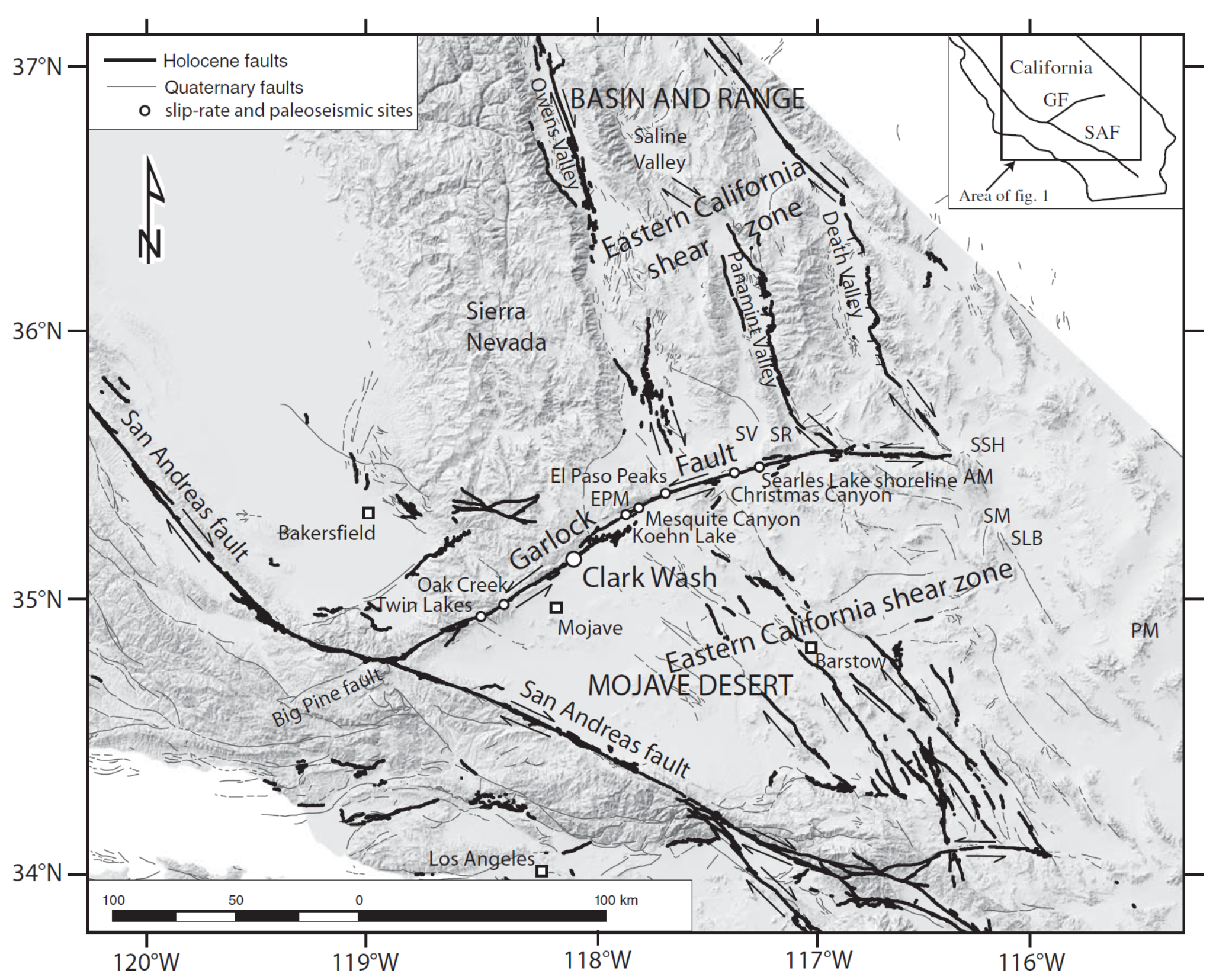
Location of the Clark Wash site (large white circle) as well as other slip-rate and paleoseismic sites (small white circles) along the Garlock fault. AM—Avawatz Mountains; EPM—El Paso Mountains; GF—Garlock fault; PM—Providence Mountains; SAF—San Andreas fault; SLB—Soda Lake Basin; SM—Soda Mountains; SR—Slate Range; SSH—Salt Spring Hills; SV—Searles
Valley.
- These authors used a variety of observations to derive a statistical estimate (using probabilistic model) for a slip rate based on an estimate of offset and radiocarbon age (which both had a range of probabilities, plotted as a probability density function). This is really cool.
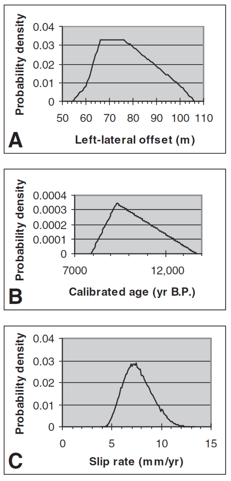
Probability density functions for left-lateral offset (A) and age (B) of Clark Wash that were assigned on the basis of quantitative constraints and subjective judgment (see text), and the resulting probability density function for the slip rate of the Garlock fault (C).
- Here is a compilation of their slip rate estimates (McGill et al., 2009).
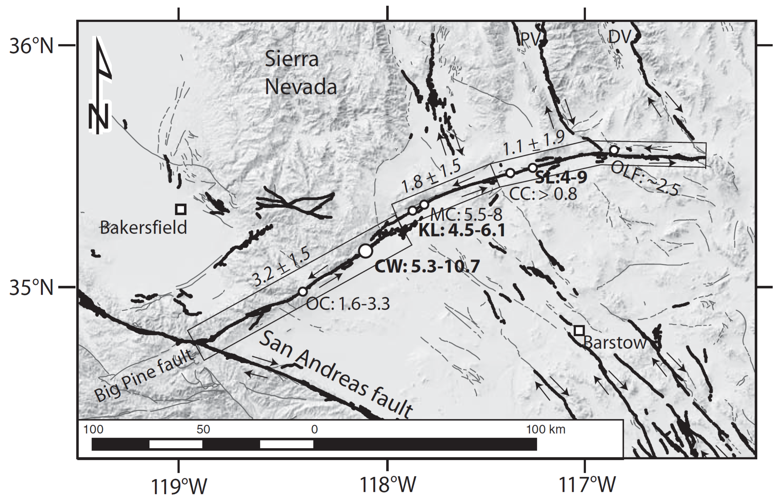
Comparison of slip-rate estimates for the Garlock fault. The three values in italics, associated with boxes that outline sections of the fault, are the slip rates and formal uncertainties from Meade and Hager’s (2005) best-fitting elastic block model of available geodetic data. They report, however, that experience with a range of models suggests that true uncertainties are ~3 mm/yr. White-filled circles mark the locations of Holocene and Late Quaternary geologic slip-rate estimates. The Holocene rates that are constrained by radiocarbon dates and are thus considered most reliable are shown in bold […].
* more abbreviations and explanation in the paper
Background Literature – Owens Valley fault
- Kylander-Clark et al. (2005) use the lateral offset of plutonic dikes (igneous rocks) to constrain a long term slip rate across the Owens Valley fault. This map shows one of the dike pairs used in their analysis. By knowing the age of these dieks, and the distance that they have been offset, we can obtain a slip rate.
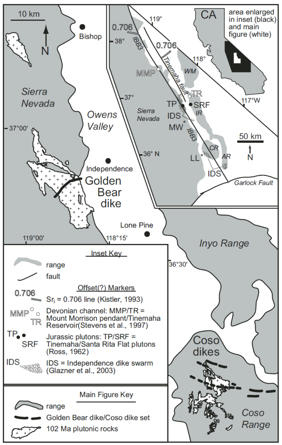
Locations of the Golden Bear and Coso dikes, adjacent to Owens Valley. Main figure shows the Golden Bear and Coso dikes striking into the valley, where they intrude 102 Ma plutons. Both the dikes and the plutons provide distinctive markers that can be matched across the valley and are consistent with 65 km of dextral displacement since 84 Ma. Inset shows other markers across Owens Valley that earlier workers suggested indicate from 0 to 65 km of dextral offset across the valley. Also shown are the traces of the Tinemaha fault (Stevens et al., 1997; Stevens and Stone, 2002) and intrabatholithic break 3 (IBB3; Kistler, 1993), which are hypothesized to accommodate offset of these markers. Note that the section of IBB3 between 38°N and 36.5°N is correlative with the eastern intrabatholithic break (EIB) of Saleeby and Busby (1993). Not all known locations of Independence dikes are indicated. Instead, patterned areas show only the densest parts of the dike swarm as defi ned by Glazner et al. (2003). AR—Argus Range; CR—Coso Range; IR—Inyo Range; WM—White Mountains
- Bacon and Pezzopane used trench excavations across earthquake faults to construct a prehistoric earthquake history for the Owens Valley fault. Below is their tectonic map for the region.

(A) Map of major Quaternary faults in the northern Eastern California shear zone and southern and central Walker Lane, as well as the locations of the Owens Valley fault. Faults are modified from Reheis and Dixon (1996) and Wesnousky (2005)
(B) Generalized fault and geology map of south-central Owens Valley, showing the A.D. 1872 Owens Valley fault rupture and major fault zones in the valley (modified from Hollett et al. [1991] and Beanland and Clark [1994]).
(For fault abbreviations, see their paper.)
- This map shows a more detailed view of the Owens Valley fault and the Owens Lake topography (Bacon and Pezzopane, 2007).
- This map shows the Bacon and Pezzopane (2007) field sites.

Shaded relief map of southern Owens Valley showing fault zones and the ages of the most recent prominent highstands and recessional shorelines of Owens Lake during the latest Quaternary (modified from Bacon et al., 2006).
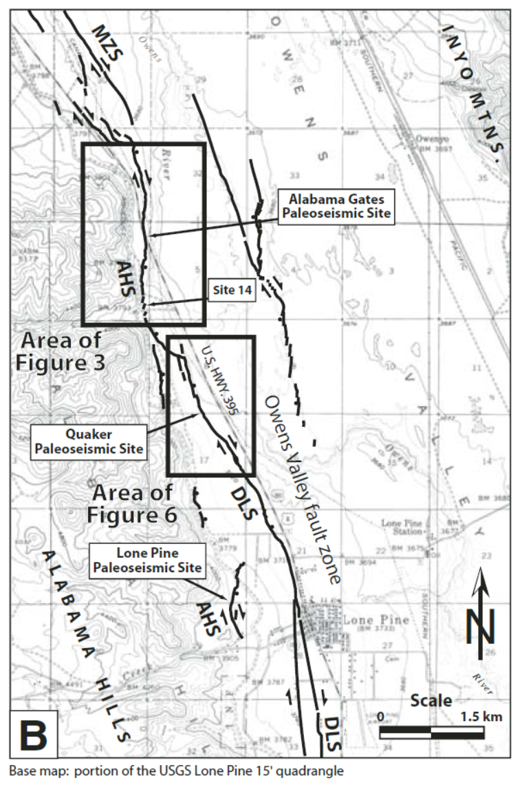
Map of the field area and locations of paleoseismic study sites in relation to the A.D. 1872 Owens Valley earthquake fault trace near Lone Pine. Study sites are located on the Alabama Hills (AHS), Diaz Lake (DLS), and Manzanar (MZS) sections of the Owens Valley fault zone mapped by Bryant (1988) and Beanland and Clark (1994) from 1:12,000 aerial photographs.
- An essential part of any earthquake fault investigation is knowledge about the geologic units that are offset by the fault. Bacon and Pezzopane (2007) also described and interpreted the sediment stratigraphy in southern Owens Valley as part of their research.
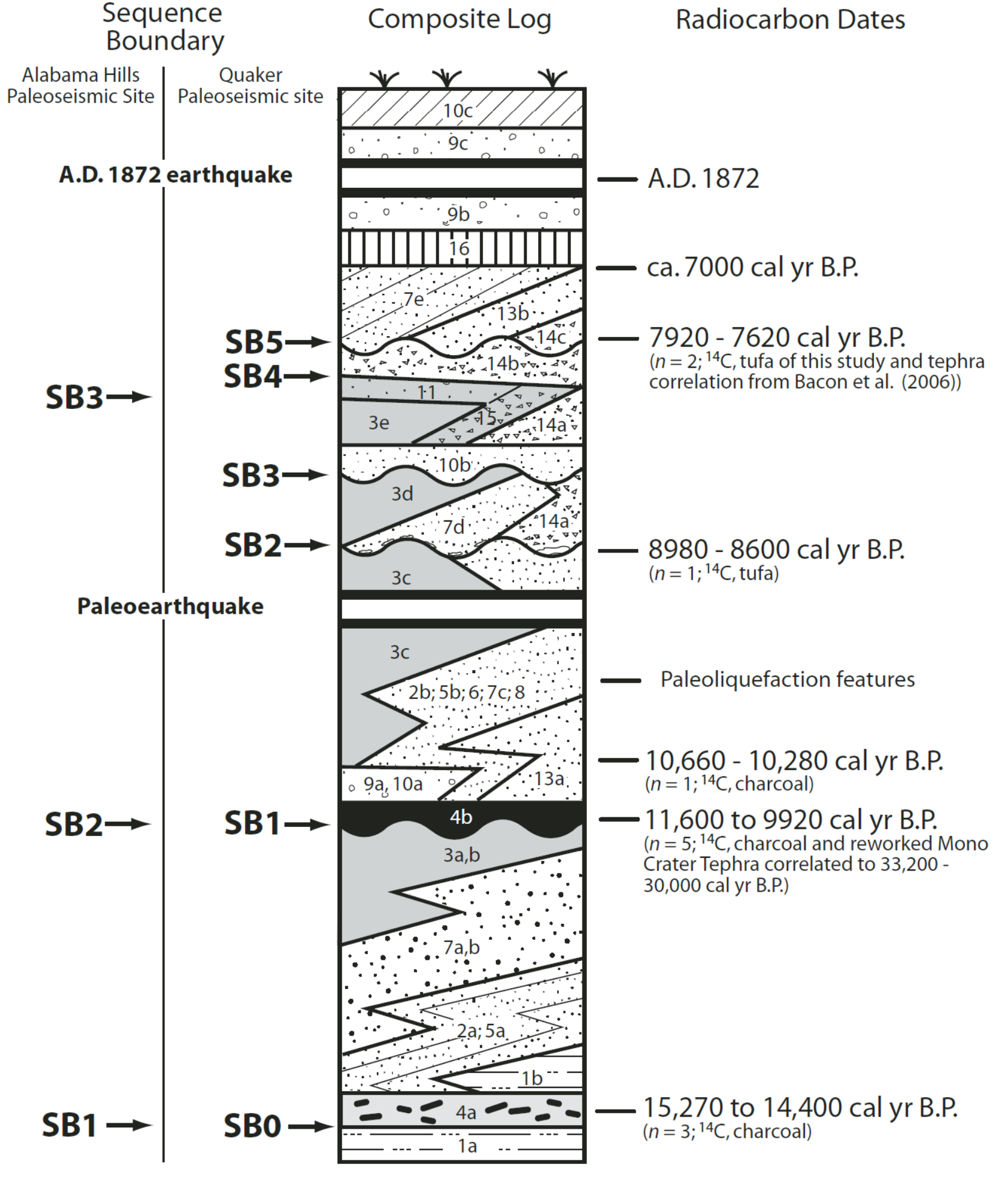
Schematic composite stratigraphic column. The generalized stratigraphic and geochronologic relations, developed from exposures at the Alabama Gates and Quaker paleoseismic sites and Owens River bluffs near Lone Pine (Bacon et al., 2006), show the positions of radiocarbon dates, sequence boundaries, and event chronologies as discussed in the text.
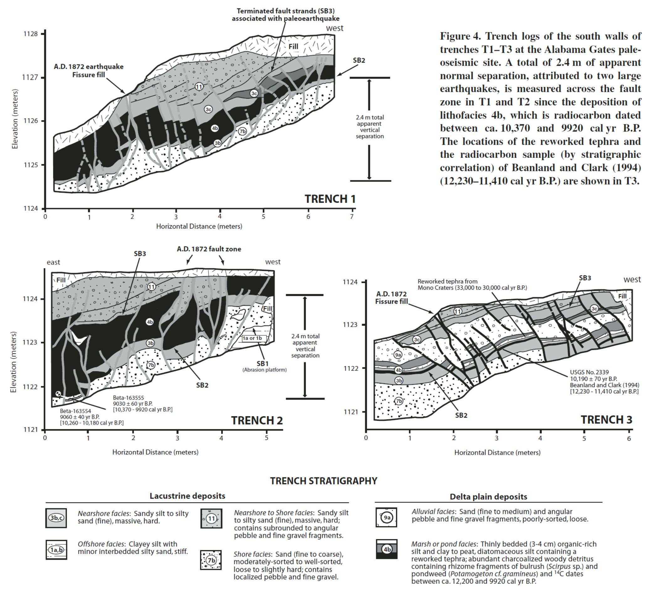
- The geologic method (McCalpin, 1996) is based on the offset of geologic materials like sedimentary deposits or bedrock lithologic units. Below are trench logs showing the geologic units that Bacon and Pezzopane (2007) use to infer an earthquake history. Geologic evidence is “primary” evidence for earthquakes.
- Here is a time series showing the sedimentary and earthquake history as interpreted by Bacon and Pezzopane (2007).
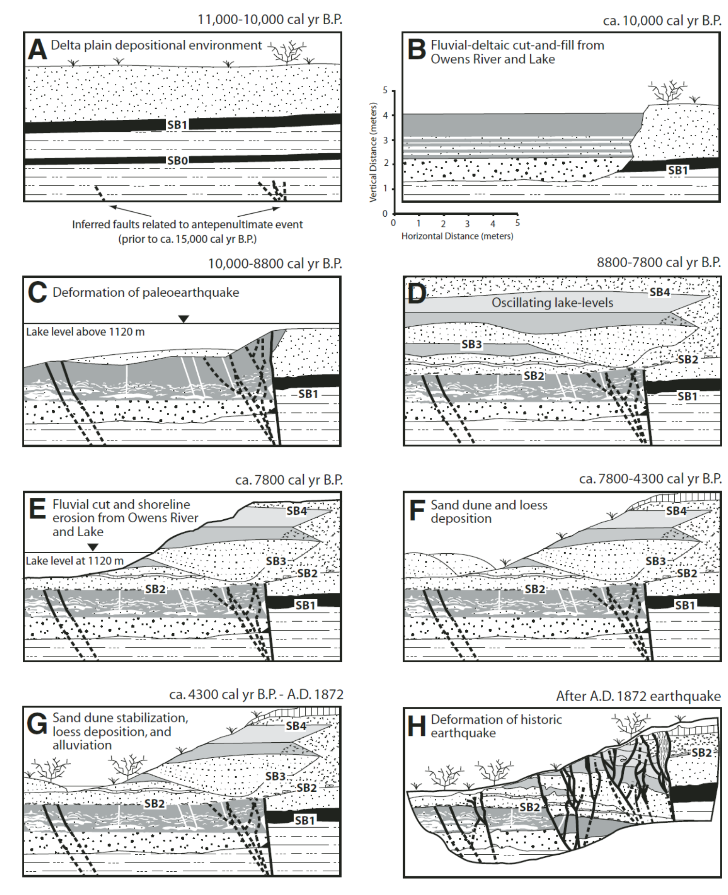
Schematic depiction of stratigraphy and structural relations at the Quaker paleoseismic site prior to the penultimate event and after the A.D. 1872 earthquake (depictions A–H). The stratigraphy and structure exposed in trench T5 (Fig. 7) was retrodeformed and reconstructed one event at a time (while also accounting for other stratigraphic and
paleoseismic relations exposed in adjacent fault trenches and stratigraphic pits). The locations of sequence boundaries (SB0–SB4) are shown and can be referenced on Figure 5.
Background Literature – Earthquake History
- Here are the results of the paleoseismic (prehistoric earthquake history) investigation for the Owens Valley fault (Bacon and Pezzopane, 2007).

Fault segmentation and section map of central and southern Owens Valley showing overlap and possible distributive faulting and linkage between the northern segment of the Owens Valley fault (OVF) and southern White Mountains fault (WMF) near Big Pine. The trace of the A.D. Owens Valley fault rupture and section boundaries of Beanland and Clark (1994) and segment boundaries of dePolo et al. (1991) are shown in relation to the central and southern White Mountains fault and the location of the Black Mountain rupture of dePolo (1989). RRF—Red Ridge fault; LP—Lone Pine; I—Independence; BP—Big Pine; OSL—optically stimulated luminescence; PE—Penultimate event; APE—antepenultimate event; MRE—most recent event.
- McGill and Rockwell (1998) and Dawson et al. (2003) used fault trenching near El Paso Peaks, California to conduct a paleoseismic investigation along the Garlock fault. Below is a map that shows their trench site relative to tectonic features in the region.

Map showing the location of the trench site along the Garlock fault. Mountains are shaded, and valleys are shown open. Stippled areas are dry lake beds. SAF is San Andreas fault, DV is Death Valley, QM is Quail Mountains, LTC is Lone Tree Canyon, and SL is Searles (dry) Lake. Modified from McGill and Sieh [1993].
- McGill and Rockwell (1998) present this figure that shows an aerial image and a geologic map showing topographic features labeled in the aerial image. Note how there is a stream channel that is left-laterally offset.

Geomorphic and geologic expression ofthe Garlock fault at the trench site. (top) An annotated aerial photograph (courtesy U.S. Geological Survey) showing the trench site and selected geomorphic features. Unlabeled arrows mark the locations of fault scarps and benches. (bottom) A geologic map of the same area. Scale and orientation of the air photo are the same as shown on the map.
- Here is an annotated aerial image that was acquired when the light from the sun was at an angle that highlights the topographic features. This low-angle sun aerial photography method was pioneered by Bert Slemmons, one of the fathers of paleoseismology (who advised my HSU professor, Gary Carver when Gary was a student).
- Note how some features on the north side of the fault are to the left of features on the south side of the fault. This is why we call these left-lateral strike-slip faults. If one turns the image upside down, they will notice that the stuff on the other side of the fault still moves to the left. So, it does not matter what side of the fault one is standing on. I rotated the image below so we can see this first hand (see how features on the top of the image are offset to the left compared to the bottom of the image.
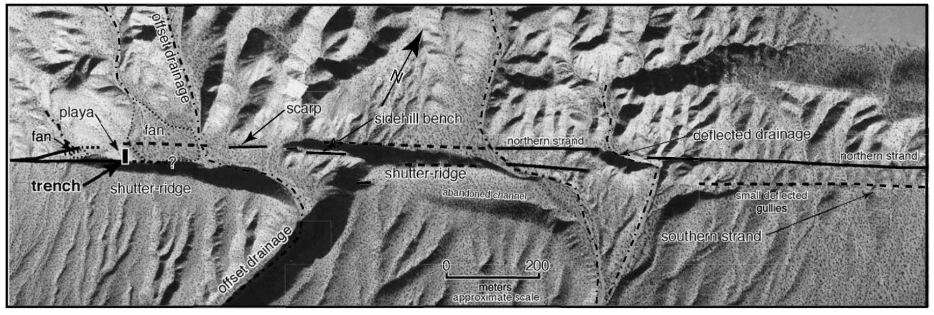
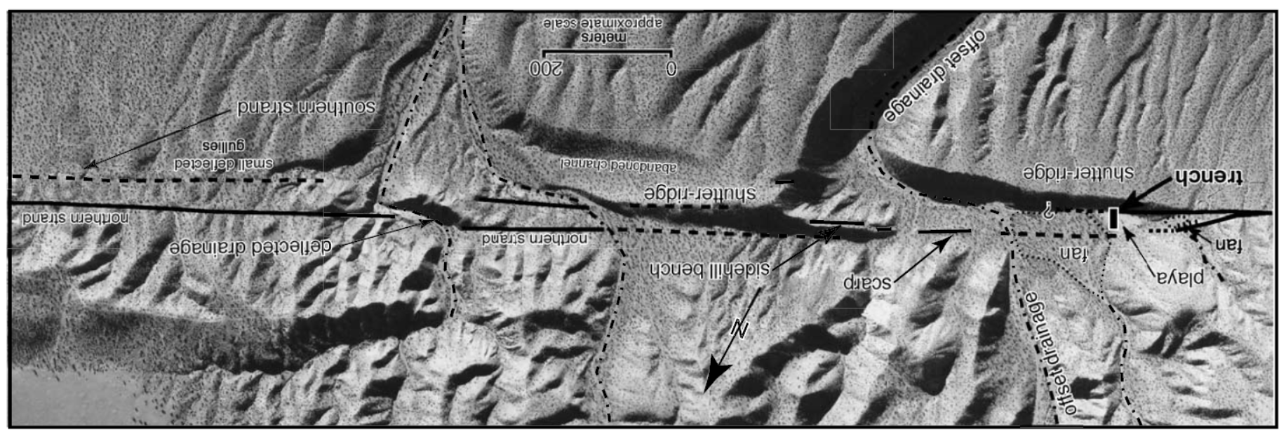
Annotated aerial photograph showing local tectonic geomorphology of the trench site. Scale is approximate. Solid lines are mappable fault traces, and dashed lines are inferred fault traces.
- This photo shows how huge and impressive the fault trenches were that Dawson et al. (2003) excavated for this study. Note the heavy equipment for scale. Read their paper to see the impressive amount of details that they used to unravel the earthquake history.
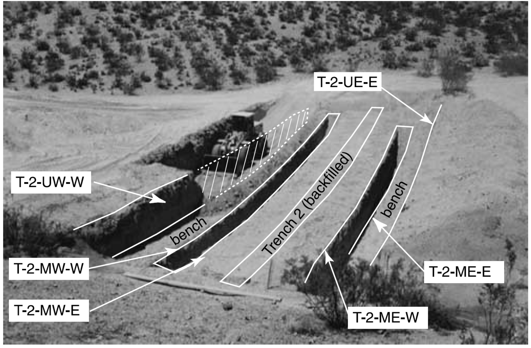
Annotated photograph illustrating some of the additional exposures that were created and documented. Note the location of trench 2, which had been backfilled at the time this photograph was taken. Trench 2 was later reexcavated to create the final and deepest exposure.
- This is but one example of the complicated sediment stratigraphy and faulting evidence that Dawson et al. (2003) used as a basis for their observations and interpretations. I show both the trench log (artwork) and the annotated panchromatic photo mosaic.
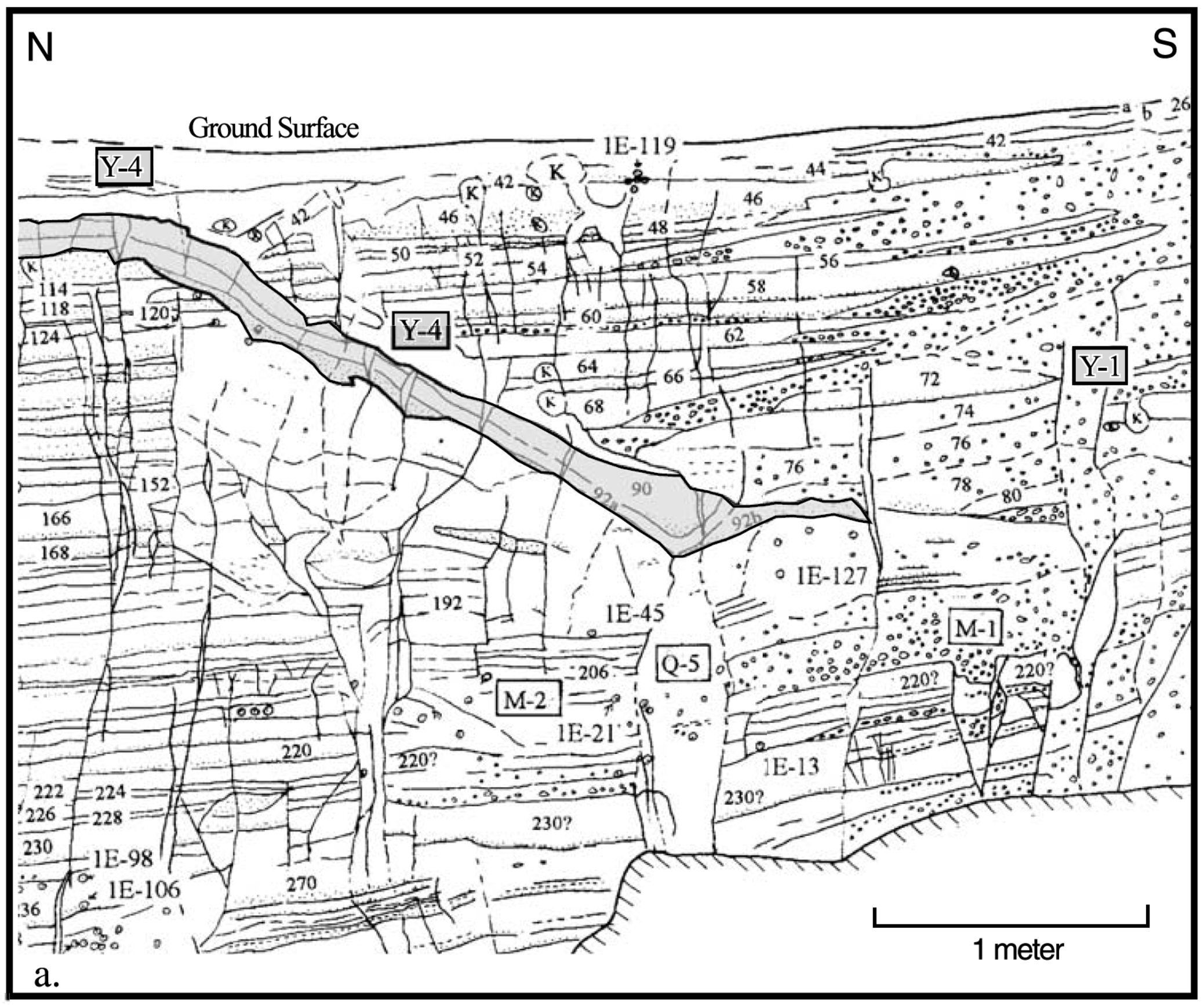
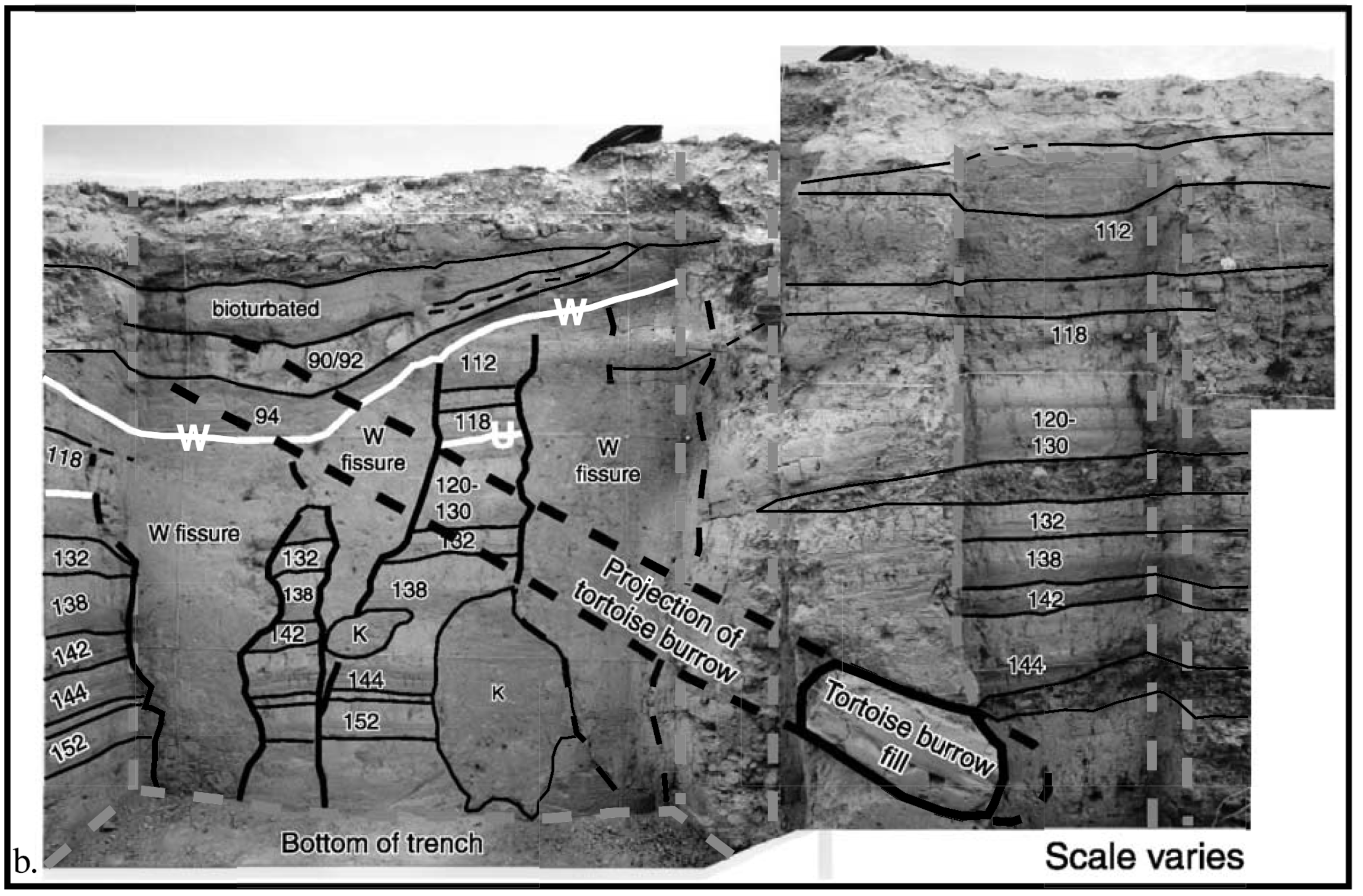
Event Y logs and three-dimensional excavation. Figure 7a is a log of a portion of trench 1 with evidence for event Y taken from McGill and Rockwell [1998]. Units shown shaded were interpreted to have been deposited in a collapse pit and then subsequently faulted by event Y. Figure 7b shows the three-dimensional excavation of this feature that shows units 90 and 92 actually being tubular in shape and units 78–42 correlative with units outside of the interpreted collapse feature. Scale varies in this mosaic due to three-dimensionality of the exposure, but the total width of the area shown is about 2.5 m. Dashed lines represent corners of 3-D exposure.
- These are complicated figures, yet elegant (McGill and Rockwell, 1998; Dawson et al., 2003). My favorite type of figure. The horizontal axis is time in calendar years (now is on the right and the past is on the left). The vertical axis is the thickness of the sedimentary deposits, with the ground surface at the top.
- Each earthquake is named an event (e.g. Event W). The dots represent radiocarbon ages (and the horizontal lines are the uncertainty associated with these ages). In the Dawson figure, the gray region represents the envelope of possible ages for the sediments between the radiocarbon ages. They assume a linear sedimentation rate between ages. Often people call these radiocarbon dates, but they are ages (it is not possible to obtain a date from radiocarbon age determinations because a date is a single day and these analyses are not that precise).

Variation of calibrated radiocarbon dates with stratigraphic depth. Errors shown are 2-sigma. The thick, diagonal line connecting the best estimates of most of the radiocarbon ages illustrates the simplest sedimentation rate history. Thinner, diagonal lines on either side represent the 2-sigma error envelope on the sedimentation rate, assuming that the date of each sample closely approximates its time of deposition. The faulting events visible within the trench are labelled along the right side of the graph, according to their stratigraphic depth; implied, preferred ages are plotted explicitly. Uncertain events are shown in parentheses. Stratigraphic depths to the earthquake horizons and to each depositional unit containing a radiocarbon sample were taken from the composite stratigraphic section shown in Figure 4.

Variation of calibrated radiocarbon dates with stratigraphic depth. Errors on the calibrated radiocarbon dates are 2-sigma. The curve connecting the solid circles connects the best estimates of the radiocarbon ages, providing the sedimentation rate. The dashed lines give the 2-sigma error envelope on the sedimentation rate.
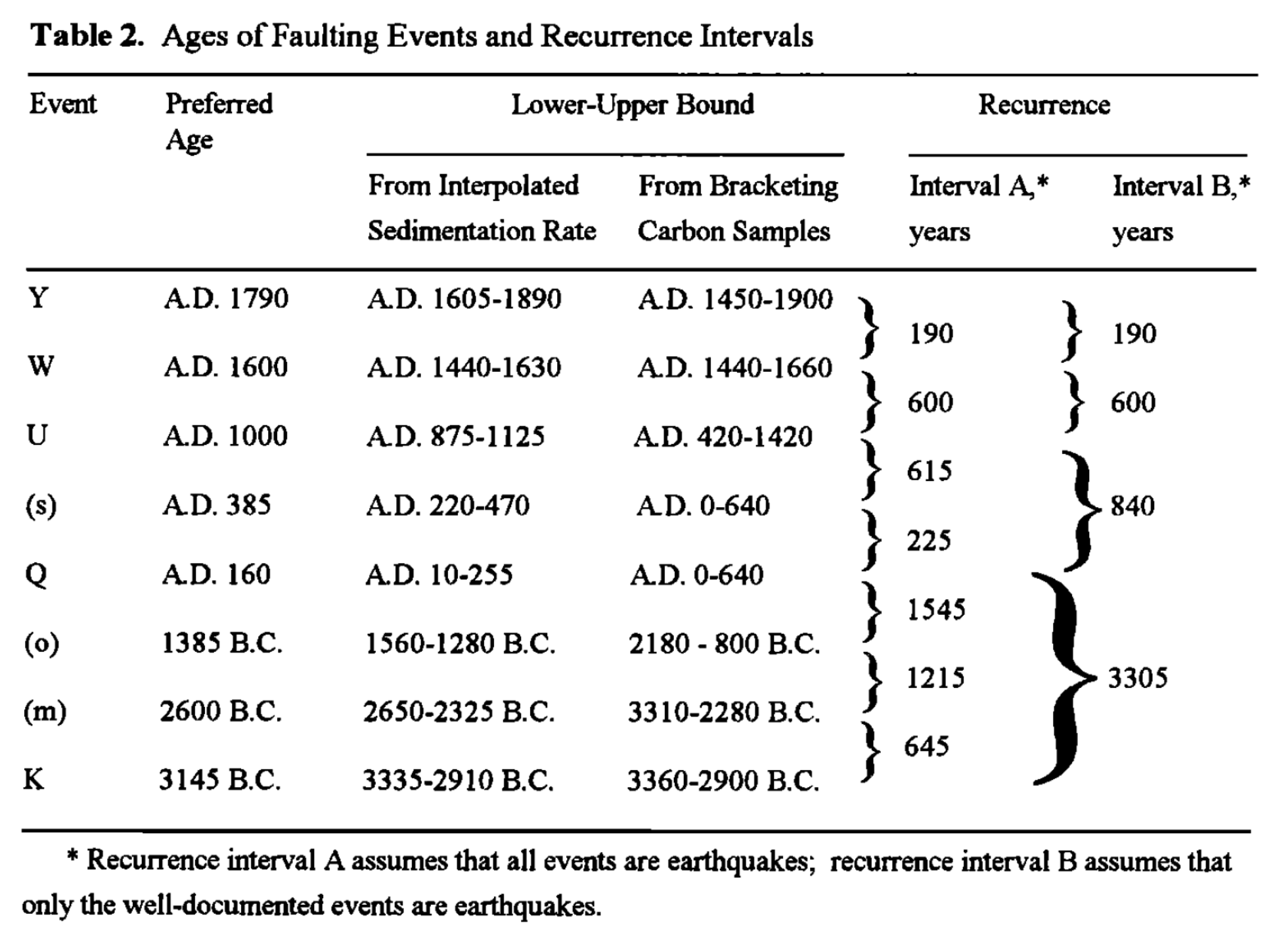
- Here is a table showing McGill and Rockwell (1998) earthquake event times and return interval for each prehistoric earthquake.
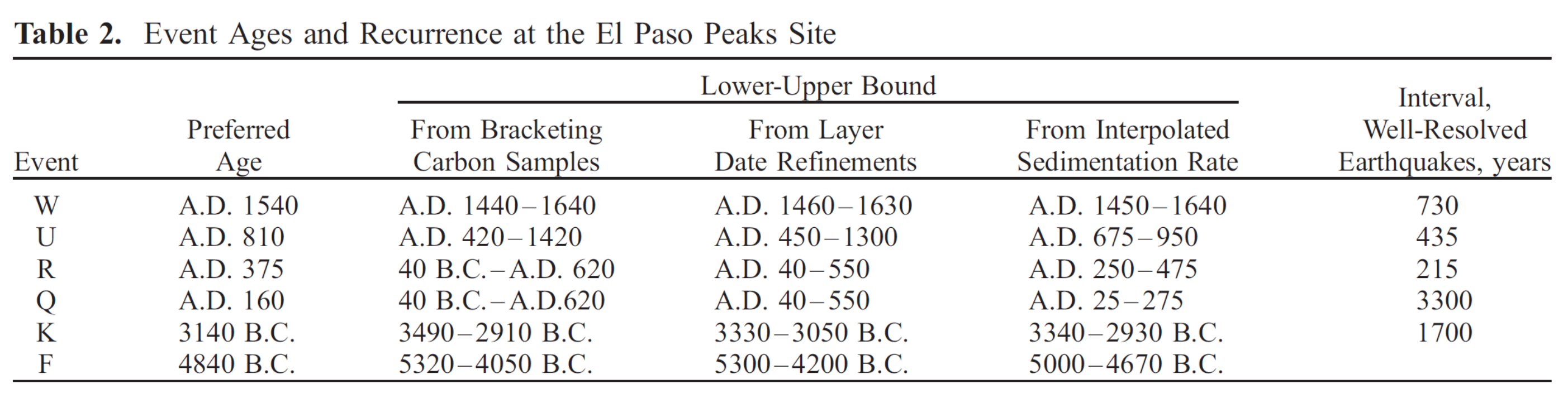
- Here is the summary of prehistoric earthquake event times for this part of the Garlock fault (Dawson et al., 2003).
- 1906.04.18 M 7.9 San Francisco
- 2017.12.14 M 4.3 Laytonville
- 2016.11.06 M 4.1 Laytonville, CA
- 2016.11.03 M 3.8 Laytonville, CA
- 2016.08.10 M 5.1 Lake Pillsbury, CA
- 2015.08.30 M 3.6 Mendocino County, CA
- 2015.07.27 M 3.5 Point Arena, CA
- 2018.07.30 M 3.7 San Pablo Bay
- 2018.01.04 M 4.4 Berkeley
- 2019.07.04 M 6.4 Ridgecrest
- 2019.07.05 M 6.4 / 7.1 Ridgecrest Update #1
- 2019.07.18 M 6.4 / 7.1 Ridgecrest Update #2
- 2019.07.20 M 6.4 / 7.1 Ridgecrest Update #3
- 2016.02.23 M 4.9 Bakersfield
- 2015.12.30 M 4.4 San Bernardino, CA
- 2015.05.03 M 3.8 Los Angeles, CA
- 2015.04.13 M 3.3 Los Angeles, CA
- 2014.04.01 M 5.1 La Habra p-3
- 2014.03.29 M 5.1 La Habra p-2
- 2014.03.28 M 5.1 La Habra p-1
- 2016.08.04 M 4.5 Honey Lake, CA
San Andreas fault
General Overview
Earthquake Reports
Northern CA
Central CA
Southern CA
Eastern CA
- 2019.06.05 M 4.3 San Clemente Island
- 2018.04.05 M 5.3 Channel Islands
- 2018.04.05 M 5.3 Channel Islands Update #1
- 1994.11.17 M 6.7 Northridge, CA
- 1971.02.09 M 6.7 Sylmar, CA
Southern CA
Earthquake Reports
Social Media (UPDATE 2019.07.21
It was an unexpected surprise today when we ran into Roger Bilham in the field. He joined us for a few hours mapping a cross fault south of the M7.1 rupture. This fault that may be an important part of the puzzle of why the rupture stopped where it did. pic.twitter.com/bzQWoO4Mdn
— Tim Dawson (@timblor) July 19, 2019
Surface rupture and relative co-seismic right-lateral movement on the main fault trace of the Mw 7.1 #RidgecrestEarthquake. Images Google Earth & DigitalGlobe (2018-2019). pic.twitter.com/NvWp4rbDQN
— Sotiris Valkaniotis (@SotisValkan) July 19, 2019
And some more clear data of horizontal displacement (using CosiCorr) #Ridgecrestearthquakes fault ruptures. Dark gradient lines mark in detail the surface rupture trace – notice width of fault zone at southeast (Imagery from GoogleEarth/DigitalGlobe@2019) pic.twitter.com/0xMGDZTfP4
— Sotiris Valkaniotis (@SotisValkan) July 19, 2019
Southern part of Ridgecrest #earthquakes surface rupture now on Google Earth (you should use image timeline tool)
Amazing righ-lateral offsets of small gullies here. pic.twitter.com/aKVrMR1YQM— Robin Lacassin (@RLacassin) July 19, 2019
And the horizontal displacement results / image correlation (#MicMac) for #Ridgecrestearthquakes surface rupture, comparing pre- and post-eq high-res imagery. Profiles show coseismic offset (Not super-accurate – Imagery from GoogleEarth/DigitalGlobe@2019) pic.twitter.com/l7VlLZdhEM
— Sotiris Valkaniotis (@SotisValkan) July 19, 2019
Identified a few places where the #RidgecrestEarthquake ruptured some sort of underground pipelines that lead to leak of fuel or water. Possible #leak points are exactly on the main surface rupture (1-4m displacement). Images from Google Earth pic.twitter.com/aeZM9xees8
— Sotiris Valkaniotis (@SotisValkan) July 19, 2019
Another view of Ridgecrest #earthquakes right-lateral surface rupture from Google Earth (with image timeline tool) pic.twitter.com/4qgYuFcw8p
— Robin Lacassin (@RLacassin) July 19, 2019
A few more detailed views of the #RidgecrestEarthquake surface ruptures. Displacement from image correlation (with CosiCorr, using GoogleEarth & DigitalGlobe imagery) at two sites; complex faulting, main fault trace (NW-SE) is not linear or single, NE-SW ruptures also visible. pic.twitter.com/hszT17ZYEY
— Sotiris Valkaniotis (@SotisValkan) July 19, 2019
California sees a constant, irregular rhythm of earthquakes, many too small to feel. The larger quakes near Los Angeles earlier this month were two 2 heavy beats in an ongoing pattern, ones that set off thousands of others in the area. https://t.co/k51QNx94nk pic.twitter.com/Coq5ljDTYL
— The New York Times (@nytimes) July 19, 2019
That was then, this is now! This is totally not your grandfather's earthquake response. Women have been out there doing great stuff, from instrumentation to geology to communications. Just a few of the geotweeps involved: @GeoGinger @DonyelleDavis @earthquakemom @FaultyAndSalty pic.twitter.com/GShIn1EbY9
— Susan Hough (@SeismoSue) July 19, 2019
The Geotechnical Extreme Events Reconnaissance (GEER) Association report for the Ridgecrest Earthquake Sequence is now online. #RidgecrestEarthquake @USGSBigQuakes @CalConservation #CAgeologicalSurvey and @UCLAengineering collaboration w/@USNavy https://t.co/OQwenwYM2x pic.twitter.com/zBlkAaksMR
— Jason "Jay" R. Patton (@patton_cascadia) July 20, 2019
High resolution displacement from image correlation using pre- and post- eq Google Earth images The July 4 #RidgecrestEarthquake Mw 6.4 rupture is visible in detail, up to the junction with the Mw7.1 NW-SE rupture. A lot of noise/errors but even w/ GE can identify fault features. pic.twitter.com/VYxy53TiZ6
— Sotiris Valkaniotis (@SotisValkan) July 20, 2019
A new possible scenario that involves more than 3 fault plane sources with @esa #sentine1 @unavco GPS @IRIS_EPO data.
Thanks @patton_cascadia for your report 2 and @SotisValkan for your S-2 maps! #RidgecrestEarthquake #@FraxInSAR @maferp_13 @SimoneAtzori73 @USGS pic.twitter.com/DUe8dDp5vk— Vincenzo De Novellis (@VDN75) July 20, 2019
Spent a few more days in the Ridgecrest area this week mapping and measuring fault rupture south of Hwy 178. Found where the main strand offset Pinnacles Road. Parked the @Jeep right on the fault because I like to live dangerously! pic.twitter.com/pUIfAMmvTz
— Brian Olson (@mrbrianolson) July 20, 2019
Awesome GIF showing a before & after image of the surface faulting from the #RidgecrestEarthqauke. The dark staining is water from a pipeline that was broken by the ground shifting 2-3 feet sideways on the other side of the fault. Thank you @SotisValkan for the imagery. pic.twitter.com/HZTG3Aks0Q
— Brian Olson (@mrbrianolson) July 20, 2019
Sub cm-scale cracks observed today along the Garlock Fault in a few locations…also multiple relatively low altitude drones flight for high-res 3D mapping, oh, and a desert tortoise too. #RidgecrestEarthquake #drones #SfM pic.twitter.com/DwiN09i3F8
— Robert Leeper (@whatsbelow) July 21, 2019
A 3D view of the central NW-SE rupture w/offsets from image correlation. View towards E-SE pic.twitter.com/uHmHSeaAgx
— Sotiris Valkaniotis (@SotisValkan) July 21, 2019
This is not about Ridgecrest, but about the time, 20 June.
Apollo 11-16 installed seismometers recording moonquakes from '69 to '77. Four kinds were identified: (1) deep moonquakes (700km deep); (2) impact of meteorites; (3) thermal quakes caused by the expansion because of sun; and (4) shallow moonquakes (20km deep). #Apollo50th pic.twitter.com/oWoNfBFP0a
— iunio iervolino (@iuniervo) July 20, 2019
UPDATE 2020.12.09
Taking a deeper look into using USDA NAIP imagery for optical correlation – Ridgecrest 2019 earthquake. Advantages of NAIP; open public data, high resolution (0.6m), pre-processed/orthorectified & ready to use. N-S component shows only minimal artifacts from mosaicking. 1/4 pic.twitter.com/E0C9rTEZvu
— Sotiris Valkaniotis (@SotisValkan) December 9, 2020
- Amos, C.B., Bwonlee, S.J., Hood, D.H., Fisher, G.B., Bürgmann, R., Renne, P.R., and Jayko, A.S., 2013. Chronology of tectonic, geomorphic, and volcanic interactions and the tempo of fault slip near Little Lake, California in GSA Bulletin, v. 125, no. 7-8, https://doi.org/10.1130/B30803.1
- Astiz, L. and Allen, C.R., 1983. Seismicity of the Garlock Fault, California in BSSA v. 73, no. 6, p. 1721-1734
- Bacon, S.N. and Pezzopane, S.K., 2007. A 25,000-year record of earthquakes on the Owens Valley fault near Lone Pine, California: Implications for recurrence intervals, slip rates, and segmentation models in GSA Bulletin, v. 119, no. 7/8, p. 823-847, https://doi.org/10.1130/B25879.1
- Bakun, W.H., Ralph A. Haugerud, Margaret G. Hopper, Ruth S. Ludwin, 2002. The December 1872 Washington State Earthquake in BSSA, v. 92, no. 8., https://doi.org/10.1785/0120010274
- Brocher, T., Margaret G. Hopper, S.T. Ted Algermissen, David M. Perkins, Stanley R. Brockman, and Edouard P. Arnold, 2048. Aftershocks, Earthquake Effects, and the Location of the Large 14 December 1872 Earthquake near Entiat, Central Washington in BSSA, v. 108, no. 1., https://doi.org/10.1785/0120170224
- Chuang, R.Y. and Johnson, K.M., 2011. Reconciling geologic and geodetic model fault slip-rate discrepancies in Southern California: Consideration of nonsteady mantle flow and lower crustal fault creep in Geology, v. 39, no. 7, p. 627630, https://doi.org/10.1130/G32120.1
- Dawson, T. E., S. F. McGill, and T. K. Rockwell, Irregular recurrence of paleoearthquakes along the central Garlock fault near El Paso Peaks, California, J. Geophys. Res., 108(B7), 2356, https://doi.org/10.1029/2001JB001744, 2003.
- Dixon, T.H., Norabuena, E., and Hotaling, L., 2003. Paleoseismology and Global Positioning System: Earthquake-cycle effects and geodetic versus geologic fault slip rates in the Eastern California shear zone in Geology, v. 31, no. 1., p. 55-58,
- Frankel, K.L., Glazner, A.F., Kirby, E., Monastero, F.C., Strane, M.D., Oskin, M.E., Unruh, J.R., Walker, J.D., Anandakrishnan, S., Bartley, J.M., Coleman, D.S., Dolan, J.F., Finkel, R.C., Greene, D., Kylander-Clark, A., Morrero, S., Owen, L.A., and Phillips, F., 2008, Active tectonics of the eastern California shear zone, in Duebendorfer, E.M., and Smith, E.I., eds., Field Guide to Plutons, Volcanoes, Faults, Reefs, Dinosaurs, and Possible Glaciation in Selected Areas of Arizona, California, and Nevada: Geological Society of America Field Guide 11, p. 43–81, doi: 10.1130/2008.fl d011(03).
- Frisch, W., Meschede, M., Blakey, R., 2011. Plate Tectonics, Springer-Verlag, London, 213 pp.
- Gan, W., Zhang, P., Shen, Z-K., Prescott, W.H., and Svarc, J.L., 2003. Initiation of deformation of the Eastern California Shear Zone: Constraints from Garlock fault geometry and GPS observations in GRL, v. 30, no. 10, https://doi.org/10.1029/2003GL017090
- Guest, B., Pavlis, T.L., Goldberg, H., and Serpa, L., 2003. Chasing the Garlock: A study of tectonic response to vertical axis rotation in Geology, v. 31, no. 6, p. 553-556
- Hayes, G., 2018, Slab2 – A Comprehensive Subduction Zone Geometry Model: U.S. Geological Survey data release, https://doi.org/10.5066/F7PV6JNV.
- Holt, W. E., C. Kreemer, A. J. Haines, L. Estey, C. Meertens, G. Blewitt, and D. Lavallee (2005), Project helps constrain continental dynamics and seismic hazards, Eos Trans. AGU, 86(41), 383–387, , https://doi.org/10.1029/2005EO410002. /li>
- Kreemer, C., J. Haines, W. Holt, G. Blewitt, and D. Lavallee, 2000. On the determination of a global strain rate model, Geophys. J. Int., 52(10), 765–770.
- Kreemer, C. , W.E. Holt, and A.J. Haines, 2002. The global moment rate distribution within plate boundary zones. In S. Stein and J.T. Freymueller (eds.): Plate Boundary Zones, Geodynamics Series, Vol. 30, https://doi.org/10/1029/030GD10
- Kreemer, C., W. E. Holt, and A. J. Haines, 2003. An integrated global model of present-day plate motions and plate boundary deformation, Geophys. J. Int., 154(1), 8–34, , https://doi.org/10.1046/j.1365-246X.2003.01917.x.
- Kreemer, C., G. Blewitt, E.C. Klein, 2014. A geodetic plate motion and Global Strain Rate Model in Geochemistry, Geophysics, Geosystems, v. 15, p. 3849-3889, https://doi.org/10.1002/2014GC005407.
- Kylander-Clark, A.R.C., Coleman, D.S., Glazner, A.F., and Bartley, J.M., 2005. Evidence for 65 km of dextral slip across Owens Valley, California, since 83 Ma in GSA Bulletin, v. 117, no. 7/8, https://doi.org/10.1130/B25624.1
- McAuliffe, L. J., Dolan, J. F., Kirby, E., Rollins, C., Haravitch, B., Alm, S., & Rittenour, T. M., 2013. Paleoseismology of the southern Panamint Valley fault: Implications for regional earthquake occurrence and seismic hazard in southern California. Journal of Geophysical Research: Solid Earth, 118, 5126-5146, https://doi.org/10.1029/jgrb.50359.
- McGill, S.F. and Rockwell, T., 1998. Ages of late Holocene earthquakes on the central Garlock fault near El Paso Peaks, California in JGR, v. 103, no. B4, p. 7265-7279
- McGill, S.F., Wells, S.G., Fortner, S.K., Kuzma, H.A., and McGill, J.D., 2009. Slip rate of the western Garlock fault, at Clark Wash, near Lone Tree Canyon, Mojave Desert, California in GSA Bulletin, v. 121, no. 3/4, https://doi.org/10.1130/B26123.1
- Meyer, B., Saltus, R., Chulliat, a., 2017. EMAG2: Earth Magnetic Anomaly Grid (2-arc-minute resolution) Version 3. National Centers for Environmental Information, NOAA. Model. https://doi.org/10.7289/V5H70CVX
- Müller, R.D., Sdrolias, M., Gaina, C. and Roest, W.R., 2008, Age spreading rates and spreading asymmetry of the world’s ocean crust in Geochemistry, Geophysics, Geosystems, 9, Q04006, https://doi.org/10.1029/2007GC001743
- Oskin, M. and Iriondo, A., 2004. Large-magnitude transient strain accumulation on the Blackwater fault, Eastern California shear zone in Geology, v. 32, no. 4, https://doi.org/10.1130/G20223.1
- Oskin, M., L. Perg, D. Blumentritt, S. Mukhopadhyay, and A. Iriondo, 2007. Slip rate of the Calico fault: Implications for geologic versus geodetic rate discrepancy in the Eastern California Shear Zone, J. Geophys. Res., v. 112, B03402, https://doi.org/10.1029/2006JB004451
- Oskin, M., Perg, L., Shelef, E., Strane, M., Gurney, E., Singer, B., and Zhang, X., 2008. Elevated shear zone loading rate during an earthquake cluster in eastern California in Geology, v. 36, no. 6, https://doi.org/10.1130/G24814A.1
- Peltzer, G., Crampe, F., Hensely, S., and Rosen, P., 2001. Transient strain accumulation and fault interaction in the Eastern California shear zone in geology, v. 29, no. 11
- Petersen, M.D. and Wesnousky, S.G., 1994. Review Fault Slip Rates and Earthquake Histories for Active Faults in Southern California in BSSA, v. 84, no. 5, p. 1608-1649
- Stein, R.S., Earthquake Conversations, Scientific American, vol. 288, 72-79, January issue, 2003. Republished in: Our Ever Changing Earth, Scientific American, Special Edition, v. 15 (2), 82-89, 2005.
- Toda, S., Stein, R. S., Richards-Dinger, K. & Bozkurt, S. Forecasting the evolution of seismicity in southern California: Animations built on earthquake stress transfer. J. Geophys. Res. 110, B05S16 (2005) https://doi.org/10.1029/2004JB003415
References:
Return to the Earthquake Reports page.
Roquemore, Zellmer, Simila?
Roquemore, G., 1980, Structure, tectonics, and stress field of the Coso Range,
Inyo County, California: Journal of Geophysical Research, v. 85, p. 2434–
2440.
Roquemore, G., 1988, Revised estimates of slip-rate on the Little Lake Fault,
California: Geological Society of America Abstracts with Programs, v.
20, no. 3, p. 225.
Roquemore, G., Simila, G.W., and Mori, J., 1996, The 1995 Ridgecrest earthquake sequence: new clues to the neotectonic development of the Indian
Wells Valley and the Cos Range, eastern California: Geological Society
of America Abstracts with Programs, v. 28, no. 5, p. 106.
Roquemore, G., and Zellmer, J., 1983a, Ground cracking associated with the
1982 Magnitude 5.2 Indian Wells Valley earthquake: California Geology,
v. 36, p. 197–200.
Roquemore, G., and Zellmer, J., 1983b, Tectonics, Seismicity, and volcanism
at the Naval Weapons Center: Naval Research Reviews, v. 35, p. 3–9.
Roquemore, G.R., 1981, A hypothesis to explain anomalous structures in the
western Basin and Range Province: US Geological Survey Open File
Report, 81-0503.
Roquemore, G.R., 1984, Ground magnetic survey in the Coso Range, California: Journal of Geophysical Research, v. 89, p. 3309–3314.
Roquemore, G.R., 1987, The microseismicity of the shallow geothermal reservoir in the Coso Range, California: Seismological Research Letters,
v. 58, p. 29.
Roquemore, G.R., and Simila, G.W., 1994, Aftershocks from the 28 June 1992
Landers earthquake, northern Mojave Desert to the Coso volcanic field,
California: Bulletin of the Seismological Society of America, v. 84,
p. 854–862
-
Thanks!!!! (sorry I missed these comments from July! I was pretty busy surveying surface rupture..)