I was finally getting around to writing a report for the deep Bolivia earthquake (Bolivia report here), when a M 5.3 earthquake struck offshore of the channel islands (south of Santa Cruz Island, west of Los Angeles). As is typical when an earthquake hits a populated region in the USA, the USGS websites stopped working (for the earthquakes in South America I was researching). After about half an hour or so, the websites started working again (the M 5.3 earthquake website never had a problem).
The Los Angeles region is dominated by the tectonics associated with the North America – Pacific transform plate boundary system of the San Andreas fault (SAF). The SAF accommodates the majority of plate motion between these two plates. There are sister faults where some of the plate boundary motion also goes. This plate boundary extends from the Pacific Ocean eastwards to Utah (the Wasatch fault system).
The SAF is considered a “mature” strike-slip fault because it is straight along most of the system. We think that strike-slip faults start out as smaller faults that develop as tectonic strain enters a region that is different from prior strain. As time passes, these smaller faults join each other, to align with the great circle aligned to the euler pole (the axis of rotation for plates).
The SAF does bend in some places, most notably in southern CA. This bend creates complexities in the fault, but also results in north-south compression (and thrust faults) forming the Transverse Ranges north of the LA Basin. Recent work by the California Geological Survey has been focusing on these thrust faults as they strike (trend) through Hollywood. These thrust faults are oriented east-west.
There are also additional faults offshore of LA in what is called the borderlands. Many of these faults are sub-parallel to the SAF. The best example is the Newport Inglewood fault (NIF), the locus of the 1933 Long Beach Earthquake. This fault is offshore, but also extends onshore. The NIF is generally a northwest-southeast striking right lateral strike-slip fault just like the SAF.
Some of the east-west faults also extend offshore. Onshore, they are generally thrust faults, but less is known about what they do offshore (i.e. they could have some strike-slip motion too).
Today’s earthquake happened south of Santa Catalina Island, where there is a major fault system that runs through the island: the Santa Cruz Island fault. This fault is mostly a left-lateral strike-slip fault, with a small portion of reverse (compression) motion (Pinter et al, 1998, 2001).
To the north of SC Island, is the Santa Barbara Basin, an oceanic basin that preserves an excellent record of flood and earthquake triggered sedimentary deposits.
If today’s M 5.3 is possibly related to the faults that form the Santa Cruz Basin. I provide some maps of this region below the interpretive poster. Based upon the work conducted by Schindler for their MS Thesis, Today’s earthquake appears associated with the East Santa Cruz Basin fault system (supporting that this was a left-lateral strike-slip earthquake). This is not included in the USGS active fault and fold database, but today’s earthquake suggests that it could be added.
These sedimentary basins are most likely formed from extension when the orientation of strike slip faults is not parallel to the plate motion. These are called “pull apart” basins and are a result of “transtension.” Do an internet search for more about transtension and how pull apart basins can form.
After one reads this report, check out the update here.
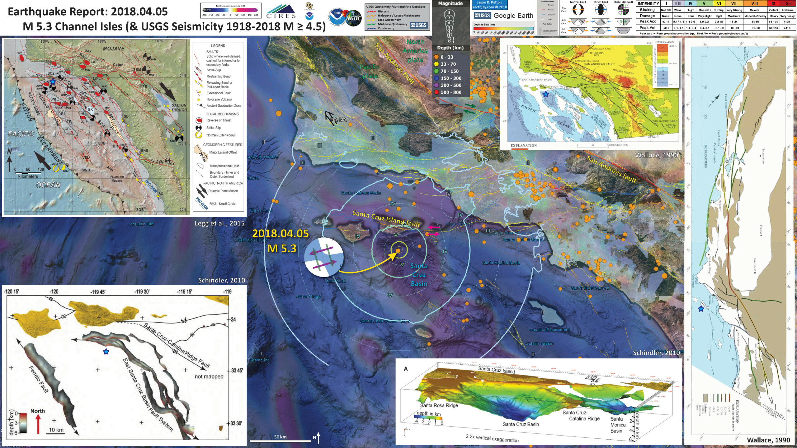
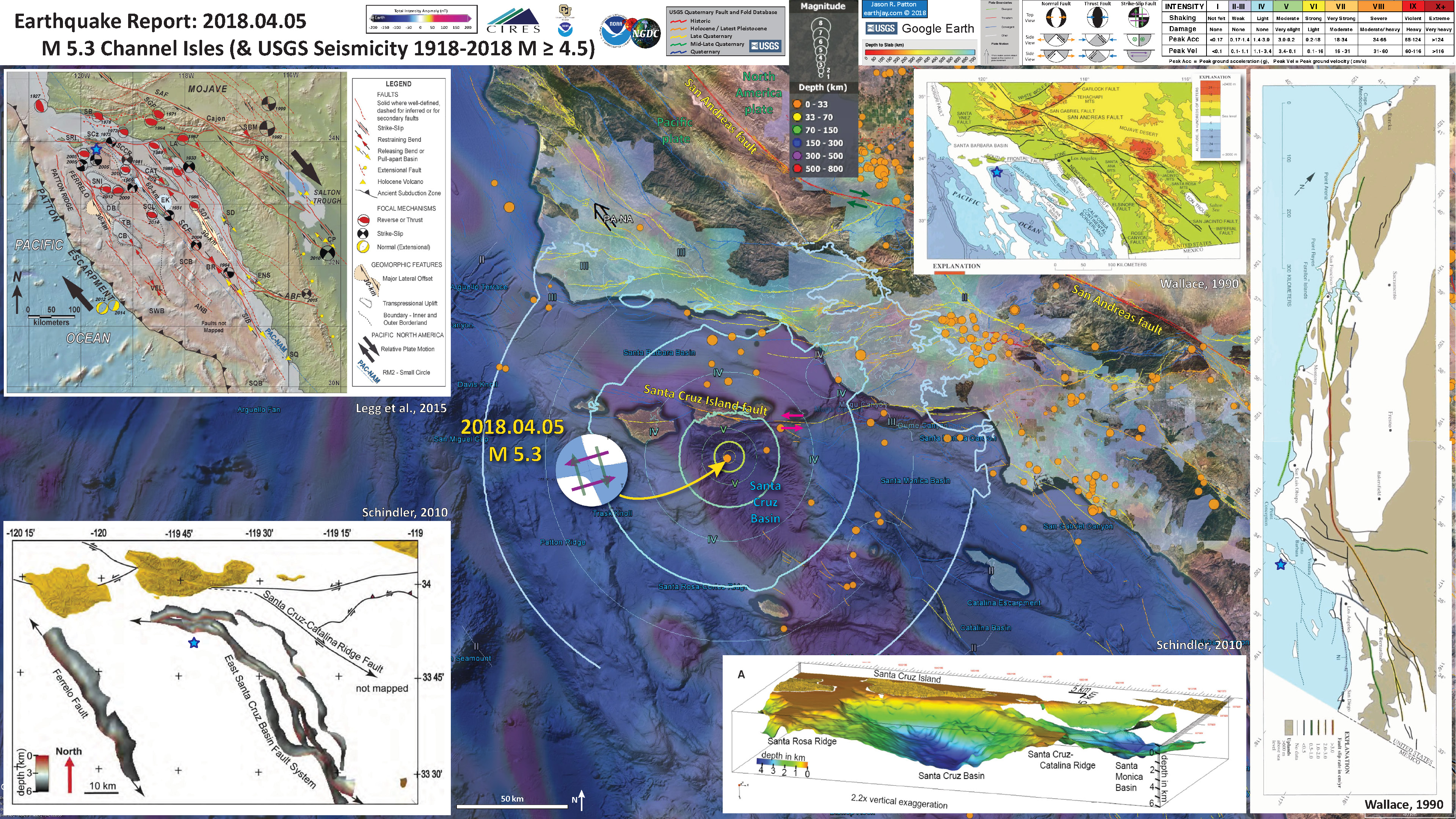
Below is my interpretive poster for this earthquake
I plot the seismicity from the past month, with color representing depth and diameter representing magnitude (see legend). I include earthquake epicenters from 1918-2018 with magnitudes M ≥ 4.5.
I plot the USGS fault plane solutions (moment tensors in blue and focal mechanisms in orange) for the M 5.3 earthquake, in addition to some relevant historic earthquakes.
- I placed a moment tensor / focal mechanism legend on the poster. There is more material from the USGS web sites about moment tensors and focal mechanisms (the beach ball symbols). Both moment tensors and focal mechanisms are solutions to seismologic data that reveal two possible interpretations for fault orientation and sense of motion. One must use other information, like the regional tectonics, to interpret which of the two possibilities is more likely.
- I also include the shaking intensity contours on the map. These use the Modified Mercalli Intensity Scale (MMI; see the legend on the map). This is based upon a computer model estimate of ground motions, different from the “Did You Feel It?” estimate of ground motions that is actually based on real observations. The MMI is a qualitative measure of shaking intensity. More on the MMI scale can be found here and here. This is based upon a computer model estimate of ground motions, different from the “Did You Feel It?” estimate of ground motions that is actually based on real observations.
-
I include some inset figures.
- On the right side of the poster are figures from Wallace (1990) and show the main faults associated with the SAF system. I place a blue star in the general location of today’s earthquake (as also in other places on this poster).
- To the upper left of the Wallace SAF map for California is a figure also from Wallace (1990) that shows more details, including elevation information (color = height or depth).
- To the lower left of the Wallace SAF map for CA is a figure that shows the high resolution bathymetry (seafloor shape) for the Santa Cruz Basin.
- In the upper left corner is a seismotectonic map of the CA Borderlands (Legg et al., 2015). They show faults and their sense of motion. There are also focal mechanisms for historic earthquakes.
- In the lower left corner is a larger scale map of this region, showing the faults as mapped by Schindler (2007).
USGS Earthquake Pages
- 2018.04.05 M 5.3 Channel Islands
These are from this current sequence
Some Relevant Discussion and Figures
- Here is the figure showing the evolution of the SAF since its inception about 29 Ma. I include the USGS figure caption below as a blockquote.
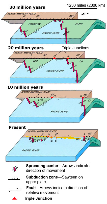
EVOLUTION OF THE SAN ANDREAS FAULT.
This series of block diagrams shows how the subduction zone along the west coast of North America transformed into the San Andreas Fault from 30 million years ago to the present. Starting at 30 million years ago, the westward- moving North American Plate began to override the spreading ridge between the Farallon Plate and the Pacific Plate. This action divided the Farallon Plate into two smaller plates, the northern Juan de Fuca Plate (JdFP) and the southern Cocos Plate (CP). By 20 million years ago, two triple junctions began to migrate north and south along the western margin of the West Coast. (Triple junctions are intersections between three tectonic plates; shown as red triangles in the diagrams.) The change in plate configuration as the North American Plate began to encounter the Pacific Plate resulted in the formation of the San Andreas Fault. The northern Mendicino Triple Junction (M) migrated through the San Francisco Bay region roughly 12 to 5 million years ago and is presently located off the coast of northern California, roughly midway between San Francisco (SF) and Seattle (S). The Mendicino Triple Junction represents the intersection of the North American, Pacific, and Juan de Fuca Plates. The southern Rivera Triple Junction (R) is presently located in the Pacific Ocean between Baja California (BC) and Manzanillo, Mexico (MZ). Evidence of the migration of the Mendicino Triple Junction northward through the San Francisco Bay region is preserved as a series of volcanic centers that grow progressively younger toward the north. Volcanic rocks in the Hollister region are roughly 12 million years old whereas the volcanic rocks in the Sonoma-Clear Lake region north of San Francisco Bay range from only few million to as little as 10,000 years old. Both of these volcanic areas and older volcanic rocks in the region are offset by the modern regional fault system. (Image modified after original illustration by Irwin, 1990 and Stoffer, 2006.)
- Here is a map that shows the shaking potential for earthquakes in CA. This comes from the state of California here. Note how Santa Cruz Island has an increased chance of hazard due to the Santa Cruz Island fault.
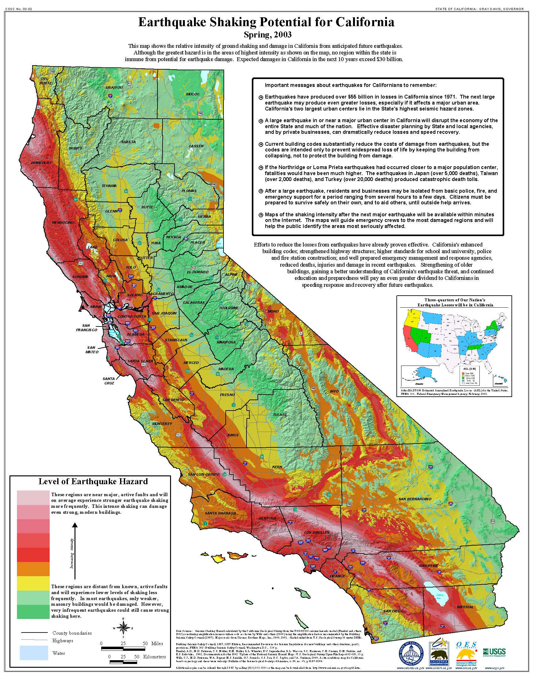
Earthquake shaking hazards are calculated by projecting earthquake rates based on earthquake history and fault slip rates, the same data used for calculating earthquake probabilities. New fault parameters have been developed for these calculations and are included in the report of the Working Group on California Earthquake Probabilities. Calculations of earthquake shaking hazard for California are part of a cooperative project between USGS and CGS, and are part of the National Seismic Hazard Maps. CGS Map Sheet 48 (revised 2008) shows potential seismic shaking based on National Seismic Hazard Map calculations plus amplification of seismic shaking due to the near surface soils.
- Here is a map that shows the tectonic provides in this region (Legg et al. (2015). While the region inherits topography and geologic structures from past tectonic regimes, the dominant tectonic control here is currently the North America – Pacific plate boundary.

Map of the California Continental Borderland showing major tectonic features and moderate earthquake locations (M >5.5). The dashed box shows area of this study. The large arrows show relative plate motions for the Pacific-North America transform fault boundary (~N40° ± 2°W; RM2 and PA-1 [Plattner et al., 2007]). BP = Banning Pass, CH = Chino Hills, CP = Cajon Pass, LA = Los Angeles, PS = Palm Springs, V = Ventura, ESC = Santa Cruz Basin, ESCBZ = East Santa Cruz Basin fault zone, SCI = Santa Catalina Island, SCL = San Clemente Island, SMB = Santa Monica Basin, and SNI = San Nicolas Island. Base map from GeoMapApp/Global Multi-Resolution Topography (GMRT) [Ryan et al., 2009].
- This shows the timeline of what has controlled the tectonics in this region (Legg et al., 2015).

Chronology of major Cenozoic events in the Southern California region (after Wright [1991] and Legg and Kamerling [2012]). Intensity of tectonic deformation is represented by the curve. Local (Los Angeles Basin) biostratigraphic zonation is shown. The slanted labels for Neogene stages represent the time-transgressive nature of these boundaries.
- Here is the figure with more details about the tectonic interpretation of the area (Legg et al., 2015)

Map showing bathymetry, Quaternary faults, and recent seismicity in the Outer Borderland. Fault locations are based on the high-resolution bathymetry, available high-resolution seismic reflection profiles, and published fault maps [cf. California Geological Survey (CGS), 2010]. The red symbols show magnitude-scaled (M>4) epicenters for seismicity recorded for the period of 1932 to 2013. Seismicity data and focal mechanisms are derived from the Southern California Seismograph Network catalogs, National Earthquake Information Center [2012–2013], and Legg [1980]. Focal mechanism event numbers correspond to Table S2 in the supporting information. The black rectangle shows location of Figure 10. The light blue lines show tracklines of multichannel seismic profiles—the labeled white profiles are shown in Figures 12 (124) and 13 (108 and 126).
- Here is the summary figure from Legg et al. (2015). This helps us put these faults systems into context.

Map showing major active tectonic elements of the northern part of the California Continental Borderland. Major active (Quaternary) faults are shown in red (SAF = San Andreas fault, ABF = Agua Blanca fault, SCF = San Clemente fault, and SCCR = Santa Cruz-Catalina Ridge, Ferrelo). Major strike-slip offsets are shown by shaded areas with estimated displacement (EK = Emery Knoll crater; Tanner Basin near DB = Dall Bank; and SDT = San Diego Trough, small pull-apart near Catalina). Other symbols show oblique fault character including transpressional restraining bends (CAT = Santa Catalina Island, CB = Cortes Bank, and TB = Tanner Bank), uplifts (SRI = Santa Rosa Island, SCz = Santa Cruz Island, SNI = San Nicolas Island, CB = Cortes Bank, TB = Tanner Bank, and SBM = San Bernardino Mountains), and transtensional pull-apart basins (SD = San Diego, ENS = Ensenada, SCB = San Clemente Basin, and SIB = San Isidro Basin). The large arrows show Pacific-North America relative plate motions with the blue dashed line (PAC-NAM) along a small circle for the RM2 [Minster and Jordan, 1978] plate motions model through San Clemente Island (SCL). Boundary between the Inner and Outer Borderland follows the East Santa Cruz Basin fault zone (dotted line; modified from Schindler [2010] and De Hoogh [2012]). Holocene volcanoes exist along the coast (SQ= San Quintín) and within the Gulf of California Rift (CP = Cerro Prieto and Obsidian Buttes, Salton Trough). Dates show year of earthquakes with mapped focal mechanisms (see Table S2 in the supporting information). SB = Santa Barbara, LA = Los Angeles, and PS = Palm Springs.
- The Santa Barbara Basin to the north has an excellent Holocene record of floods and earthquakes (Du et al., 2018). Here is a plot showing the ages of possible earthquake triggered turbidites (submarine landslide deposits) from the Santa Barbara Basin.

Probability density functions (PDFs) for the 19 turbidites (olive layers) in core MV0811-14JC and core SPR090106KC in Santa Barbara Basin generated from Bacon 2.2. Brackets show 95% confidence intervals. Estimate emergence times of the Newport-Inglewood Fault (Leeper et al., 2017) in pink, Ventura- Pitas Point Fault (Rockwell et al., 2016) in green, Ventura blind thrust fault (McAuliffe et al., 2015) in purple, Compton Thrust Fault (Leon et al., 2009) in yellow and the Goleta Slide Complex (Fisher et al., 2005)in gray. Age of slumped material in 14JC is indicated by wavy texture. (For interpretation of the references to colour in this figure legend, the reader is referred to the web version of this article.)
- As I mentioned, there is some uplift associated with compression along the Santa Cruz Island fault (Pinter et al., 2001). This plot shows uplift across the region in the form of uplifted marine terraces. This plot assumes these marine terraces were formed at the same time, so if there were no differential tectonic uplift, these lines would be horizontal.

Cross-sectional profile A-B-C on Santa Rosa Island (see Fig. 3) showing corrected terrace elevations. SRIF shows the locations of the Santa Rosa Island fault. Error bars are the sum of the ±1 s uncertainties in wave-cut platform slope and the GPS measurement errors. Note the change in vertical exaggeration between the lower and upper plots. The green curve was qualitatively fit to the T2 data in order to create the smoothest possible curve that conforms to all points; other curves are scaled versions of the T2 curve. Point spacing is too coarse and error bars too large on the other levels to show deformation details, but the scaled curves show that every measured point is consistent with the pattern measured on T2.
- This is a diagram that shows how a pull apart basin might form (Wu et al., 2009).
![]()
General characteristics of a pull-apart basin in a dextral side-stepping fault system. The pull-apart basin is defined to develop in pure strike-slip when alpha = 0 degrees and in transtension when 0 degrees < alpha 45 degrees.
- This figure shows the results of modeling in clay, showing a pull apart basin form (Wu et al., 2009).
![]()
Plan view evolution of transtensional pull-apart basin model illustrated with: (a) time-lapse overhead photography; and (b) fault interpretation and incremental basin subsidence calculated from differential laser scans. Initial and final baseplate geometry shown with dashed lines; (c) basin topography at end of experiment.
Geologic Fundamentals
- For more on the graphical representation of moment tensors and focal mechnisms, check this IRIS video out:
- Here is a fantastic infographic from Frisch et al. (2011). This figure shows some examples of earthquakes in different plate tectonic settings, and what their fault plane solutions are. There is a cross section showing these focal mechanisms for a thrust or reverse earthquake. The upper right corner includes my favorite figure of all time. This shows the first motion (up or down) for each of the four quadrants. This figure also shows how the amplitude of the seismic waves are greatest (generally) in the middle of the quadrant and decrease to zero at the nodal planes (the boundary of each quadrant).

- There are three types of earthquakes, strike-slip, compressional (reverse or thrust, depending upon the dip of the fault), and extensional (normal). Here is are some animations of these three types of earthquake faults. The following three animations are from IRIS.
Strike Slip:
Compressional:
Extensional:
Social Media
Did You Feel the M5.3 EQ that just took place off the Channel Islands, CA? Please let us know here: https://t.co/cHMIb35SOk pic.twitter.com/qhgXpT166c
— USGS (@USGS) April 5, 2018
An #earthquake just occurred on our Santa Cruz Island bald eagle camera! Watch dad & his eaglets withstand the natural disaster. pic.twitter.com/b9AQqiZEqP
— explore.org (@exploreorg) April 5, 2018
Figure 14 is a nice summary of active tectonic elements in this region: faults and recent earthquakes. Today's magnitude 5.3 seems to be similar to the 2005 magnitude 3.9 strike slip event on the Santa Rosa-Cortes Ridge (close region & focal mechanism) pic.twitter.com/Guk75RFwN3
— Lucile Bruhat (@seismolucy) April 5, 2018
Map of the felt reports received so far after M5.3 earthquake pic.twitter.com/VFUhTObCd6
— EMSC (@LastQuake) April 5, 2018
CGS @CalConservation monitoring CA coastal tide gauge recordings.
NO INDICATION of local tsunami generated from offshore M5.3 earthquake. pic.twitter.com/flm0ALVJag— Cynthia Pridmore (@earthquakemom) April 5, 2018
Overall 11000 responses to the Did You Feel It? system for today's offshore M5.3 earthquake. Remember, "not felt" reports are welcome, too: they keep the map from being too biased by a handful of remote felt reports. pic.twitter.com/2rKdoh7BxV
— Susan Hough (@SeismoSue) April 5, 2018
Webcam view of the 5.3 earlier today in SoCal, from quite near the epicenter, on Santa Cruz Island https://t.co/Wm5D7ZDx6w
— Austin Elliott (@TTremblingEarth) April 5, 2018
Earthquake eagles https://t.co/TS4tX26lBq
— Susan Hough (@SeismoSue) April 6, 2018
Offshore M5.3 apparently represented a successful test of the California earthquake early warning system: https://t.co/NOXdFnn4Q7 (also impressive given the poor station coverage near the epicenter)
— Jascha Polet (@CPPGeophysics) April 6, 2018
#Earthquake hits Santa Barbara County, CA | M5.3 https://t.co/9aXSbk6zIA pic.twitter.com/0S6T9jIfYQ
— Sismo EQ (@sismoecuador) April 6, 2018
M5.3 occurred on an unlabeled strike-slip fault in the southern California Borderland, some good visuals on the tectonics of this area can be found here:https://t.co/utfNoIywy6 pic.twitter.com/K67vLTMS8J
— Jascha Polet (@CPPGeophysics) April 6, 2018
Great animation by Dr Tanya Atwater showing the evolution of southern California, including the Channel Islands which are near today's M5.3 #earthquake. pic.twitter.com/W3dJbDZtM6
— IRIS Earthquake Sci (@IRIS_EPO) April 5, 2018
View of cliffs along Santa Cruz Island during today’s earthquake. Dust rolls off cliffs as the temblor hit close to the Island, photo taken by a private fishing boat on scene during the quake. @VCFD pic.twitter.com/1lhCo9Cwqp
— VCFD PIO (@VCFD_PIO) April 5, 2018
5.4 mag earthquake off Santa Cruz Island. Felt the shaking here in LA City Hall. Checking earthquake early warning for details. @kwhudnut @USGS pic.twitter.com/s0DW2ktOIH
— Jeff Gorell (@JeffGorell) April 5, 2018
Earthquake Early Warning System Worked, Gave Heads-Up Before 5.3 Temblor Hit Off SoCal Coast: Officials https://t.co/Ngzsr8DqeE via @ktla
— Cynthia Pridmore (@earthquakemom) April 6, 2018
. @LastQuake Woahh Californians are launching LastQuake app IMMEDIATELY after the shaking! They're real time sensors #Earthquake #California pic.twitter.com/UVfkrr9VL8
— Real News Line (@RealNewsLine) April 5, 2018
- 2017.12.14 M 4.3 Laytonville
- 2016.11.06 M 4.1 Laytonville, CA
- 2016.11.03 M 3.8 Laytonville, CA
- 2016.08.10 M 5.1 Lake Pillsbury, CA
- 2015.08.30 M 3.6 Mendocino County, CA
- 2015.07.27 M 3.5 Point Arena, CA
- 2018.01.04 M 4.4 Berkeley
- 2016.02.23 M 4.9 Bakersfield
- 2015.12.30 M 4.4 San Bernardino, CA
- 2015.05.03 M 3.8 Los Angeles, CA
- 2015.04.13 M 3.3 Los Angeles, CA
- 2014.04.01 M 5.1 La Habra p-3
- 2014.03.29 M 5.1 La Habra p-2
- 2014.03.28 M 5.1 La Habra p-1
- 2016.08.04 M 4.5 Honey Lake, CA
San Andreas fault
General Overview
Earthquake Reports
Northern CA
Central CA
Southern CA
Eastern CA
- 2018.04.05 M 5.3 Channel Islands
- 1994.11.17 M 6.7 Northridge, CA
- 1971.02.09 M 6.7 Sylmar, CA
Southern CA
Earthquake Reports
- Frisch, W., Meschede, M., Blakey, R., 2011. Plate Tectonics, Springer-Verlag, London, 213 pp.
- Hayes, G., 2018, Slab2 – A Comprehensive Subduction Zone Geometry Model: U.S. Geological Survey data release, https://doi.org/10.5066/F7PV6JNV.
- Holt, W. E., C. Kreemer, A. J. Haines, L. Estey, C. Meertens, G. Blewitt, and D. Lavallee (2005), Project helps constrain continental dynamics and seismic hazards, Eos Trans. AGU, 86(41), 383–387, , https://doi.org/10.1029/2005EO410002. /li>
- Jessee, M.A.N., Hamburger, M. W., Allstadt, K., Wald, D. J., Robeson, S. M., Tanyas, H., et al. (2018). A global empirical model for near-real-time assessment of seismically induced landslides. Journal of Geophysical Research: Earth Surface, 123, 1835–1859. https://doi.org/10.1029/2017JF004494
- Kreemer, C., J. Haines, W. Holt, G. Blewitt, and D. Lavallee (2000), On the determination of a global strain rate model, Geophys. J. Int., 52(10), 765–770.
- Kreemer, C., W. E. Holt, and A. J. Haines (2003), An integrated global model of present-day plate motions and plate boundary deformation, Geophys. J. Int., 154(1), 8–34, , https://doi.org/10.1046/j.1365-246X.2003.01917.x.
- Kreemer, C., G. Blewitt, E.C. Klein, 2014. A geodetic plate motion and Global Strain Rate Model in Geochemistry, Geophysics, Geosystems, v. 15, p. 3849-3889, https://doi.org/10.1002/2014GC005407.
- Meyer, B., Saltus, R., Chulliat, a., 2017. EMAG2: Earth Magnetic Anomaly Grid (2-arc-minute resolution) Version 3. National Centers for Environmental Information, NOAA. Model. https://doi.org/10.7289/V5H70CVX
- Müller, R.D., Sdrolias, M., Gaina, C. and Roest, W.R., 2008, Age spreading rates and spreading asymmetry of the world’s ocean crust in Geochemistry, Geophysics, Geosystems, 9, Q04006, https://doi.org/10.1029/2007GC001743
- Pagani,M. , J. Garcia-Pelaez, R. Gee, K. Johnson, V. Poggi, R. Styron, G. Weatherill, M. Simionato, D. Viganò, L. Danciu, D. Monelli (2018). Global Earthquake Model (GEM) Seismic Hazard Map (version 2018.1 – December 2018), DOI: 10.13117/GEM-GLOBAL-SEISMIC-HAZARD-MAP-2018.1
- Silva, V ., D Amo-Oduro, A Calderon, J Dabbeek, V Despotaki, L Martins, A Rao, M Simionato, D Viganò, C Yepes, A Acevedo, N Horspool, H Crowley, K Jaiswal, M Journeay, M Pittore, 2018. Global Earthquake Model (GEM) Seismic Risk Map (version 2018.1). https://doi.org/10.13117/GEM-GLOBAL-SEISMIC-RISK-MAP-2018.1
- Zhu, J., Baise, L. G., Thompson, E. M., 2017, An Updated Geospatial Liquefaction Model for Global Application, Bulletin of the Seismological Society of America, 107, p 1365-1385, https://doi.org/0.1785/0120160198
- Du, X., Hendy, I., Schimmelmann, 2018. A 9000-year flood history for Southern California: A revised stratigraphy of varved sediments in Santa Barbara Basin in Marine Geology, v. 397, p. 29-42, https://doi.org/10.1016/j.margeo.2017.11.014
- Legg, M. R., M. D. Kohler, N. Shintaku, and D. S. Weeraratne, 2015. Highresolution mapping of two large-scale transpressional fault zones in the California Continental Borderland: Santa Cruz-Catalina Ridge and Ferrelo faults, J. Geophys. Res. Earth Surf., 120, 915–942, doi:10.1002/2014JF003322.
- Pinter, N., Lueddecke, S.B., Keller, E.A., Simmons, K.R., 1998. Late Quaternary slip on the Santa Cruz Island fault, California in GSA Bulletin, v. 110, no. 6, p. 711-722
- Pinter, N., Johns, B., Little, B., Vestal, W.D., 2001. Fault-Related Folding in California’s Northern Channel Islands Documented by Rapid-Static GPS Positioning in GSA Today, May, 2001
- Schindler, C.S., 2010. 3D Fault Geometry and Basin Evolution in the Northern Continental Borderland Offshore Southern California Catherine Sarah Schindler, B.S. A Thesis Submitted to the Department of Physics and Geology California State University Bakersfield In Partial Fulfillment for the Degree of Masters of Science in Geology
- Wallace, Robert E., ed., 1990, The San Andreas fault system, California: U.S. Geological Survey Professional Paper 1515, 283 p. [https://pubs.er.usgs.gov/publication/pp1515].
References:
Basic & General References
Specific References
Return to the Earthquake Reports page.
- Sorted by Magnitude
- Sorted by Year
- Sorted by Day of the Year
- Sorted By Region