
A couple days ago there was a deep focus earthquake in the downgoing Nazca plate deep beneath Bolivia. This earthquake has an hypocentral depth of 562 km (~350 miles).
We are still unsure what causes an earthquake at such great a depth. The majority of earthquakes happen at shallower depths, caused largely by the frictional between differently moving plates or crustal blocks (where earth materials like the crust behave with brittle behavior and not elastic behavior). Some of these shallow earthquakes are also due to internal deformation within plates or crustal blocks.
As plates dive into the Earth at subduction zones, they undergo a variety of changes (temperature, pressure, stress). However, because people cannot directly observe what is happening at these depths, we must rely on inferences, laboratory analogs, and other indirect methods to estimate what is going on.
So, we don’t really know what causes earthquakes at the depth of this Bolivia M 6.8 earthquake. Below is a review of possible explanations as provided by Thorne Lay (UC Santa Cruz) in an interview in response to the 2013 M 8.3 Okhotsk Earthquake.
There are lots of examples in this region of South America for deep earthquakes. They are all extensional (normal fault) earthquakes.
One option could be “fluid-assisted faulting,” in which water is released from minerals as they change phases during faulting, thus lubricating the plates, Lay says.
But although this is a common mechanism for earthquakes between 70 and 400 kilometers deep, it’s unlikely to be the cause of this quake because the plate is significantly dewatered by the time it reaches 400 kilometers deep. Minerals releasing carbon dioxide as they are compacted could provide an alternative fluid to lubricate the fault, he says, much like water does at shallower depths.
And another possibility is that a transition in mineral form from low-pressure polymorphs (the form in which a mineral is stable at the surface) to high-pressure polymorphs (a denser form of a mineral that is stable at greater depths), gives the fault a start. According to this model, the plate subducts too quickly for the mineral to slowly transition to its denser form. The mineral will reach depths greater than where it is normally stable, and thus the transformation may be a catastrophic process, causing a jolt at 600 kilometers, which would allow for movement along the fault, Lay says.
There have been a number of deep earthquakes globally in the past several years. These include the 2013 M 8.3 in the Sea of Okhtosk, the 2015 M 7.8 along the Izu-Bonin Arc, and several along the central Andes. I present some interpretive posters for these earthquakes below.
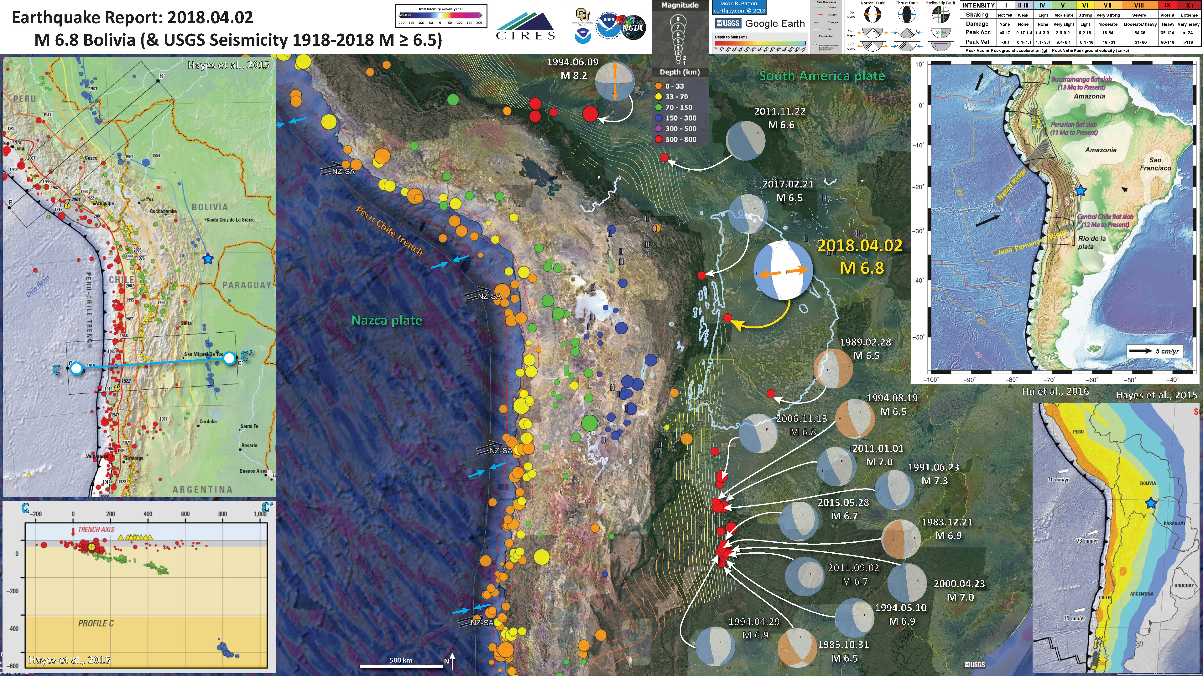
Below is my interpretive poster for this earthquake
I plot the seismicity from the past month, with color representing depth and diameter representing magnitude (see legend). I include earthquake epicenters from 1918-2018 with magnitudes M ≥ 6.5.
I plot the USGS fault plane solutions (moment tensors in blue and focal mechanisms in orange) for the M 6.8 earthquake, in addition to some relevant historic earthquakes.
I include the magnetic anomaly data (EMAG2) which helps reveal the structure of the Nazca plate.
- I placed a moment tensor / focal mechanism legend on the poster. There is more material from the USGS web sites about moment tensors and focal mechanisms (the beach ball symbols). Both moment tensors and focal mechanisms are solutions to seismologic data that reveal two possible interpretations for fault orientation and sense of motion. One must use other information, like the regional tectonics, to interpret which of the two possibilities is more likely.
- I also include the shaking intensity contours on the map. These use the Modified Mercalli Intensity Scale (MMI; see the legend on the map). This is based upon a computer model estimate of ground motions, different from the “Did You Feel It?” estimate of ground motions that is actually based on real observations. The MMI is a qualitative measure of shaking intensity. More on the MMI scale can be found here and here. This is based upon a computer model estimate of ground motions, different from the “Did You Feel It?” estimate of ground motions that is actually based on real observations.
- I include the slab contours plotted (Hayes et al., 2012), which are contours that represent the depth to the subduction zone fault. These are mostly based upon seismicity. The depths of the earthquakes have considerable error and do not all occur along the subduction zone faults, so these slab contours are simply the best estimate for the location of the fault.
-
I include some inset figures.
- In the upper right corner is a plate tectonic map from Hu et al. (2016), which shows the major plate boundaries in the region. The subduction zone is indicated as a black line with triangles (the triangles show the direction that the Nazca plate is subducting below the South America plate). I place a cyan star in the general location of this M 6.8 earthquake (as in other figures).
- In the upper left corner is a part of the map from Hayes et al. (2015) that shows historic seismicity. Below the map is a cross section showing seismicity. This is the cross section C-C’ shown on the map above in cyan.
- In the lower right corner is part of the seismic hazard map for South America (Hayes et al., 2015). Color represents the relative amount of shaking a location may experience in the next 50 years (“10% in 50 years peak acceleration”). Yellow areas may experience 1.6-3.2 m/s^2 (gravity is 9.8 m/s^2). Green may experience between 0.8-1.6 m/s^2.
USGS Earthquake Pages
- 2018.04.02 M 6.8 Bolivia
These are from this current sequence
- 2015.11.24 22:45 M 7.6 Peru
- 2015.11.24 22:50 M 7.6 Peru
- 2015.11.26 M 6.7 Brazil
- 2017.02.21 M 6.5 Bolivia
These are from earlier earthquakes
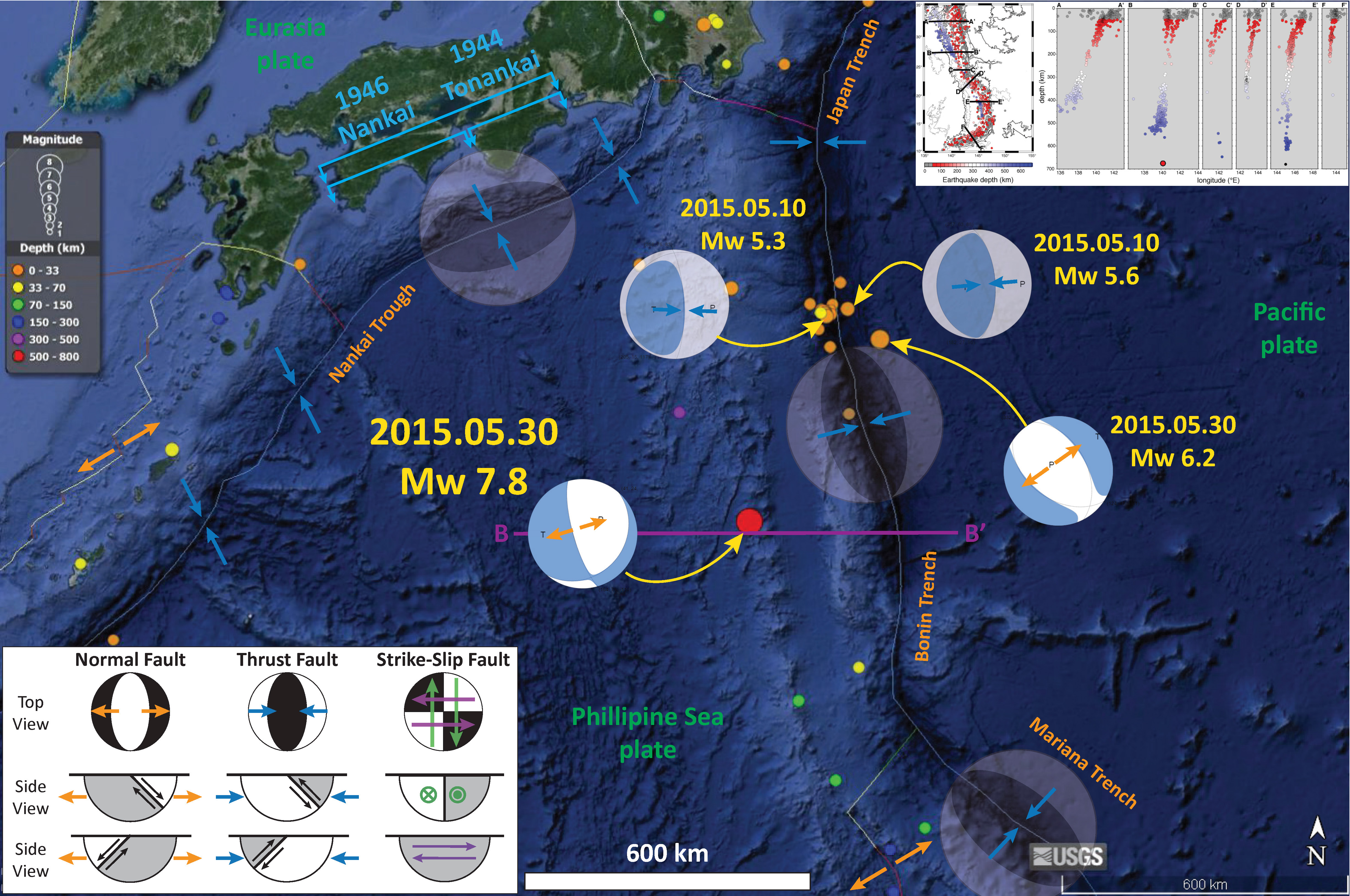
- Here is my interpretive poster for the 2015 Izu Bonin earthquake (click here for the report).
- Here is my interpretive poster for the 2015 deep Peru earthquakes. (click here for the report)

Some Relevant Discussion and Figures
- Here is an animation from IRIS that reviews the tectonics of the Peru-Chile subduction zone. For the animation, first is a screen shot and below that is the embedded video. This animation is from IRIS. Written and directed by Robert F. Butler, University of Portland. Animation and Graphics: Jenda Johnson, geologist. Consultant: Susan Beck, University or Arizona. Narration: Elayne Shapiro, University of Portland.
- Here is a download link for the embedded video below (34 MB mp4)

- The Goes et al. (2017) paper presents an excellent review of the various forces and earthquake types along subduction zones globally. This paper is open source and free to download. Below are some summary figures.
- This shows the general relations between various forces exerted on a subducting slab.
- Here is a plot showing their summary of observations for various subduction zones globally.
![]()
Schematic diagram showing the main forces that affect how slabs interact with the transition zone. The slab sinks driven by its negative thermal buoyancy (white filled arrows). Sinking is resisted by viscous drag in the mantle (black arrows) and the frictional/viscous coupling between the subducting and upper plate (pink arrows). To be able to sink, the slab must bend at the trench. This bending is resisted by slab strength (curved green arrow). The amount the slab needs to bend depends on whether the trench is able to retreat, a process driven by the downward force of the slab and resisted (double green arrow) by upper-plate strength and mantle drag (black arrows) below the upper plate. At the transition from ringwoodite to the postspinel phases of bridgmanite and magnesiowüstite (rg – bm + mw), which marks the interface between the upper and lower mantle, the slab’s further sinking is hampered by increased viscous resistance (thick black arrows) as well as the deepening of the endothermic phase transition in the cold slab, which adds positive buoyancy (open white arrow) to the slab.
By contrast, the shallowing of exothermic phase transition from olivine to wadsleyite (ol-wd) adds an additional driving force (downward open white arrow), unless it is kinetically delayed in the cold core of the slab (dashed green line), in which case it diminishes the driving force. Phase transitions in the crustal part of the slab (not shown) will additionally affect slab buoyancy. Buckling of the slab in response to the increased sinking resistance at the upper-lower mantle boundary is again resisted by slab strength.
![]()
Summary of morphologies of transition-zone slabs as imaged by tomographic studies and their Benioff stress state. Arrows on the map indicate the approximate locations of the cross sections shown around the map, with their points in downdip direction. Blue shapes are schematic representations of slab morphologies (based on the extent of fast seismic anomalies that were tomographically resolvable from the references listed). Horizontal black lines indicate the base of the transition zone (~660 km depth). For flattened slabs, the approximate length of the flat section is given in white text inside the shapes. For penetrating slabs, the approximate depth to which the slabs are continuous is given in black text next to the slabs. Circles inside the slabs indicate whether the mechanisms of earthquakes at intermediate (100–350 km) and deep (350–700 km) are predominantly downdip extensional (black) or compressional (white). Stress states are from the compilations of Isacks and Molnar (1971), Alpert et al. (2010), Bailey et al. (2012), complemented by Gorbatov et al. (1997) for Kamchatka, Stein et al. (1982) for the Antilles, McCrory et al. (2012) for Cascadia, Papazachos et al. (2000) for the Hellenic zone, and Forsyth (1975) for Scotia. The subduction zones considered are (from left to right and top to bottom): RYU—Ryukyu, IZU—Izu, HON—Honshu, KUR—Kuriles, KAM—Kamchatka, ALE—Aleutians, ALA—Alaska, CAL—Calabria, HEL—Hellenic, IND—India, MAR—Marianas, CAS—Cascadia, FAR—Farallon, SUM—Sumatra, JAV—Java, COC—Cocos, ANT—Antilles, TON—Tonga, KER—Kermadec, CHI—Chile, PER—Peru, SCO—Scotia. Numbers next to the red subduction zone codes refer to the tomographic studies used to define the slab shapes
Geologic Fundamentals
- For more on the graphical representation of moment tensors and focal mechnisms, check this IRIS video out:
- Here is a fantastic infographic from Frisch et al. (2011). This figure shows some examples of earthquakes in different plate tectonic settings, and what their fault plane solutions are. There is a cross section showing these focal mechanisms for a thrust or reverse earthquake. The upper right corner includes my favorite figure of all time. This shows the first motion (up or down) for each of the four quadrants. This figure also shows how the amplitude of the seismic waves are greatest (generally) in the middle of the quadrant and decrease to zero at the nodal planes (the boundary of each quadrant).

- There are three types of earthquakes, strike-slip, compressional (reverse or thrust, depending upon the dip of the fault), and extensional (normal). Here is are some animations of these three types of earthquake faults. The following three animations are from IRIS.
Strike Slip:
Compressional:
Extensional:
Social Media
Today's deep M6.9 Bolivia quake hanging out by itself at the bottom(?) of the subducting slab, in (relative) isolation
(Of course, let's not forget about the other deep earthquakes in the greater area such as the famous 1994 M8.2 at 650 km depth) pic.twitter.com/QgHOC1qkpX— Jascha Polet (@CPPGeophysics) April 3, 2018
- 2010.02.27 M 8.8 Earthquake Review
- 2018.04.02 M 6.8 Bolivia
- 2018.01.14 M 7.1 Peru
- 2018.01.15 M 7.1 Peru Update #1
- 2017.06.30 M 6.0 Ecuador
- 2017.04.24 M 6.9 Chile
- 2017.04.23 M 5.9 Chile
- 2016.12.25 M 7.6 Chile
- 2016.11.24 M 7.0 El Salvador
- 2016.11.04 M 6.4 Maule, Chile
- 2016.04.16 M 7.8 Ecuador
- 2016.04.16 M 7.8 Ecuador Update #1
- 2015.11.29 M 5.9 Argentina
- 2015.11.11 M 6.9 Chile
- 2015.11.24 M 7.6 Peru
- 2015.11.26 M 7.6 Peru Update
- 2015.09.16 M 8.3 Chile
- 2014.04.01 M 8.2 Chile
- 2010.02.27 M 8.8 Chile
- 1960.05.22 M 9.5 Chile
Chile | South America
General Overview
Earthquake Reports
- Chlieh et al., 2011. Interseismic coupling and seismic potential along the Central Andes subduction zone, Journal of Geophysical Research, v. 116, B12405, 21 p.
- Espurt, N., Baby, P., Brusset, S., Roddaz, M., Hermoza, W., Regard, V., Antoine, P.-O., Salas-Gismodi, R., and Bolaños, R., 2007. How does the Nazca Ridge subduction influence the modern Amazonian foreland basin? in Geology, v. 35, no. 6, p. 515-518.
- Goes, S., Agrusta, R., van Hunen, J., and Garel, F., 2017. Subduction-transition zone interaction: A review: Geosphere, v. 13, no. 3, p. 1–21, doi:10.1130/GES01476.1.
- Hayes, G. P., D. J. Wald, and R. L. Johnson, 2012. Slab1.0: A three-dimensional model of global subduction zone geometries, J. Geophys. Res., 117, B01302, doi:10.1029/2011JB008524.
- Hayes, G.P., Smoczyk, G.M., Benz, H.M., Villaseñor, Antonio, and Furlong, K.P., 2015. Seismicity of the Earth 1900–2013, Seismotectonics of South America (Nazca Plate Region): U.S. Geological Survey Open-File Report 2015–1031–E, 1 sheet, scale 1:14,000,000, http://dx.doi.org/10.3133/ofr20151031E.
- Hu, J., Liu, L., Hermosillo, A., Zhou, Q., 2016. Simulation of late Cenozoic South American flat-slab subduction using geodynamic models with data assimilation in EPSL, v. 438, p. 1-13, http://dx.doi.org/10.1016/j.epsl.2016.01.011
- Kirby, S.H., Okal, E.A., and Engdahl, E.R., 1995. The 9 June 94 Bolivian deep earthquake: An exceptional event in an extraordinary subduction zone in Geophysical Research Letters, v. 22, no. 16, p. 2233-2236.
- Silver., P.G., Beck, S.L., Wallace, T.C., Meade, C., Myers, S.C., James, D.E., and Kuehnel, R., 1995. Rupture Characteristics of the Deep Bolivian Earthquake of 9 June 1994 and the Mechanism of Deep-Focus Earthquakes in Science, v. 268, p. 69-73.
- Trabant, C., A. R. Hutko, M. Bahavar, R. Karstens, T. Ahern, and R. Aster, 2012. Data Products at the IRIS DMC: Stepping Stones for Research and Other Applications, Seismological Research Letters, 83(5), 846–854, doi:10.1785/0220120032.
- Zhan, Z., Kanamori, H., Tsai, V.C., Helmberger, D.V., and Wei, S., 2014. Rupture complexity of the 1994 Bolivia and 2013 Sea of Okhotsk deep earthquakes in Earth and Planetary Science Letters, v. 385, p. 89-96.