I have been busy working on a paleoseismic investigation of the newly identified Shively fault in northern California (in the Mendocino triple junction region).
Here is a summary of this paleoseismic investigation.
During this work, there have been several large damaging earthquakes. I will prepare Earthquake Reports for these earthquakes over the next few weeks.
This earthquake is a magnitude M 7.7 earthquake offshore of the island of Flores, Indonesia.
https://earthquake.usgs.gov/earthquakes/eventpage/us6000tkt2/executive
This region of the world is dominated by the tectonics associated with the Java subduction zone where the Australia plate subducts beneath the Sunda plate (part of Eurasia).
The megathrust subduction zone forms the Java trench south of the island of Flores, where the Australia plate dives northwards.
Along the north side of the island of Flores, there is the Flores fault. The Flores fault is a backthrust to the subduction zone and it dips to the south beneath the island.
This M 7.7 earthquake generated a local to regional tsunami that had waves on the order of one-meter locally. (Indonesia operates a large network of tide gages but they only serve data for two days, so I missed the opportunity to download these tsunami data.)
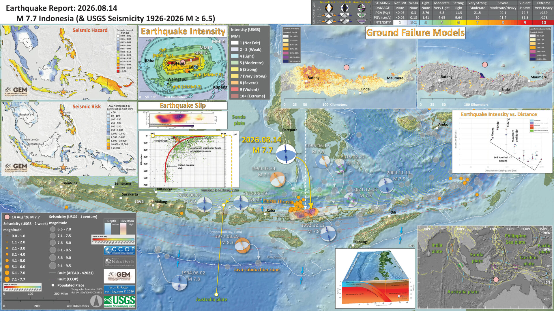
Below is my interpretive poster for this earthquake
- I plot the seismicity from the past month, with diameter representing magnitude (see legend). I include earthquake epicenters from 1925-2025 with magnitudes M ≥ 3.0 in one version.
- I plot the USGS fault plane solutions (moment tensors in blue and focal mechanisms in orange), possibly in addition to some relevant historic earthquakes.
- A review of the basic base map variations and data that I use for the interpretive posters can be found on the Earthquake Reports page. I have improved these posters over time and some of this background information applies to the older posters.
- Some basic fundamentals of earthquake geology and plate tectonics can be found on the Earthquake Plate Tectonic Fundamentals page.
- In the lower right corner is a map showing plate boundary fault lines and the major tectonic plates.
- To the left of the plate tectonic map is an inset showing a low angle oblique view of the Java subduction zone.
- In the upper left corner are maps that show the seismic hazard and seismic risk for Indonesia. I spend more time explaining this below. I place the M 7.7 epicenter on the maps as orange stars.
- In the center top-left is a map that shows earthquake intensity using the Modified Mercalli Intensity (MMI) Scale.
- To the center right is a plot that shows the same intensity (both modeled and reported) data as displayed on the map. Note how the intensity gets smaller with distance from the earthquake. I label some of the large cities, some are shown on the maps.
- In the upper right corner are two maps showing the possibility of earthquake triggered landslides and earthquake induced liquefaction for these two earthquakes.
- Below the intensity map is a view of the USGS finite fault slip model. This shows the amount that they estimate that the fault slipped during the earthquake. The fault may have slipped more than 2.5 meters. I placed an overlay of this fault slip on the main map.
- Below the fault slip model is a plot of seismicity from Hangesh and Whitney (2016). The location of this cross section is shown on the main map. One may observe that both the subduction zone and the Flores backthrust are shown on the cross section. I place the location of the M 7.7 on the cross section as an orange star.
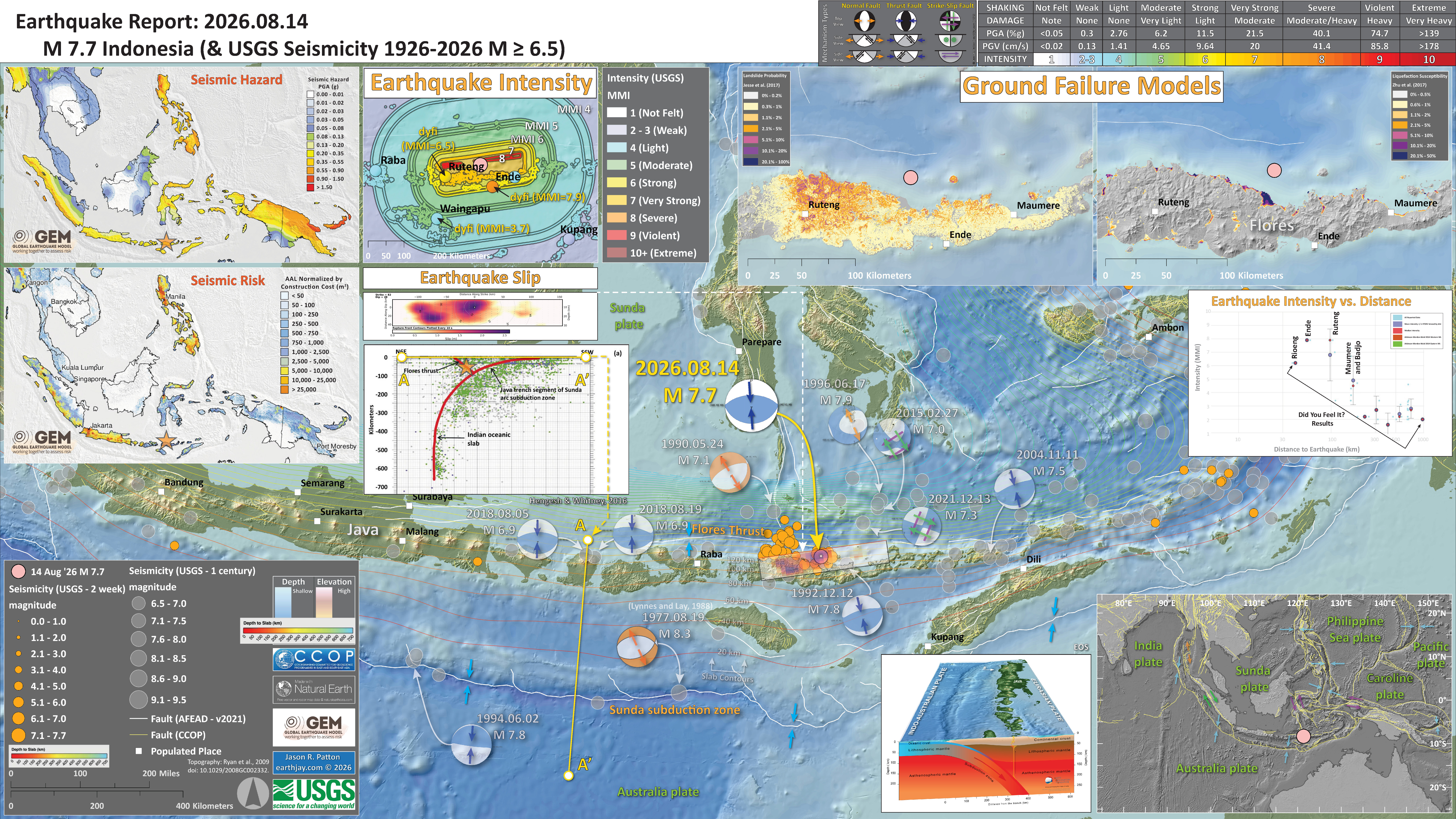
I include some inset figures. Some of the same figures are located in different places on the larger scale map below.
- Here is the map with a month’s seismicity plotted.
Other Report Pages
Shaking Intensity
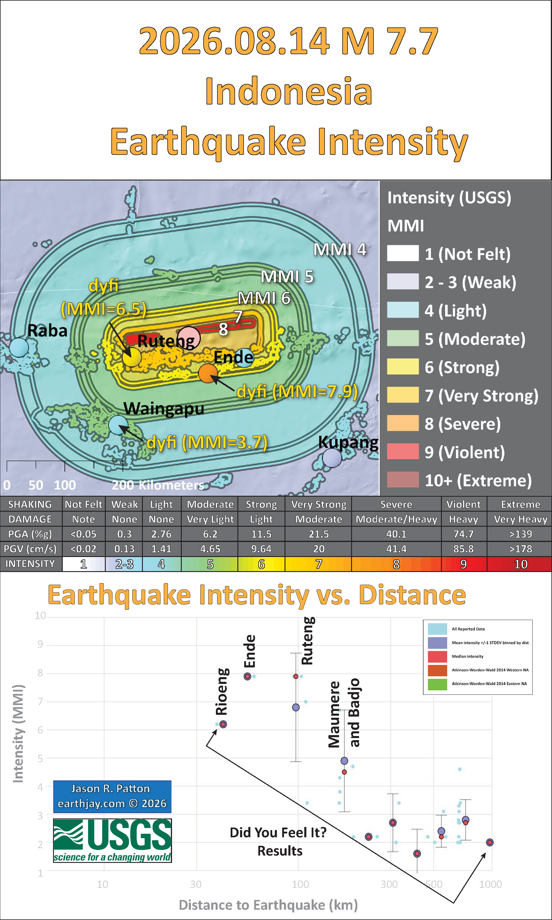
- Here is a figure that shows a more detailed comparison between the modeled intensity and the reported intensity. Both data use the same color scale, the Modified Mercalli Intensity Scale (MMI). More about this can be found here. The colors and contours on the map are results from the USGS modeled intensity. The DYFI data are plotted as colored dots (color = MMI, diameter = number of reports).
- In the upper panel is the USGS Did You Feel It reports map, showing reports as colored dots using the MMI color scale. Underlain on this map are colored areas showing the USGS modeled estimate for shaking intensity (MMI scale).
- In the lower panel is a plot showing MMI intensity (vertical axis) relative to distance from the earthquake (horizontal axis). The models are represented by the green and orange lines. The DYFI data are plotted as light blue dots. The mean and median (different types of “average”) are plotted as orange and purple dots. Note how well the reports fit the green line (the model that represents how MMI works based on quakes in California).
- Below the map and the lower plot is the USGS MMI Intensity scale, which lists the level of damage for each level of intensity, along with approximate measures of how strongly the ground shakes at these intensities, showing levels in acceleration (Peak Ground Acceleration, PGA) and velocity (Peak Ground Velocity, PGV).
Potential for Ground Failure
- Below are a series of maps that show the potential for landslides and liquefaction. These are all USGS data products.
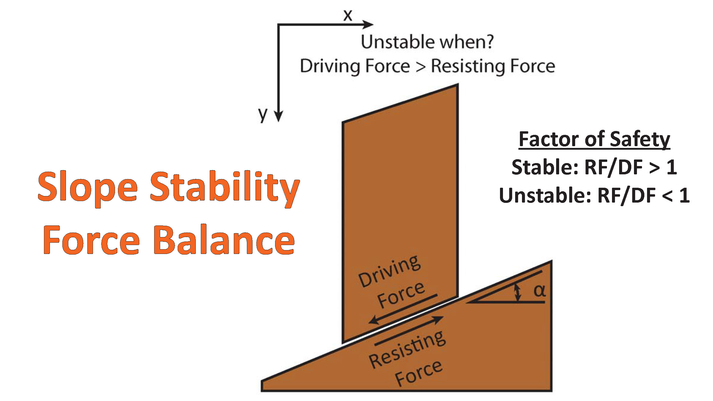
There are many different ways in which a landslide can be triggered. The first order relations behind slope failure (landslides) is that the “resisting” forces that are preventing slope failure (e.g. the strength of the bedrock or soil) are overcome by the “driving” forces that are pushing this land downwards (e.g. gravity). The ratio of resisting forces to driving forces is called the Factor of Safety (FOS). We can write this ratio like this:FOS = Resisting Force / Driving Force
- When FOS > 1, the slope is stable and when FOS < 1, the slope fails and we get a landslide. The illustration below shows these relations. Note how the slope angle α can take part in this ratio (the steeper the slope, the greater impact of the mass of the slope can contribute to driving forces). The real world is more complicated than the simplified illustration below.
- Landslide ground shaking can change the Factor of Safety in several ways that might increase the driving force or decrease the resisting force. Keefer (1984) studied a global data set of earthquake triggered landslides and found that larger earthquakes trigger larger and more numerous landslides across a larger area than do smaller earthquakes. Earthquakes can cause landslides because the seismic waves can cause the driving force to increase (the earthquake motions can “push” the land downwards), leading to a landslide. In addition, ground shaking can change the strength of these earth materials (a form of resisting force) with a process called liquefaction.
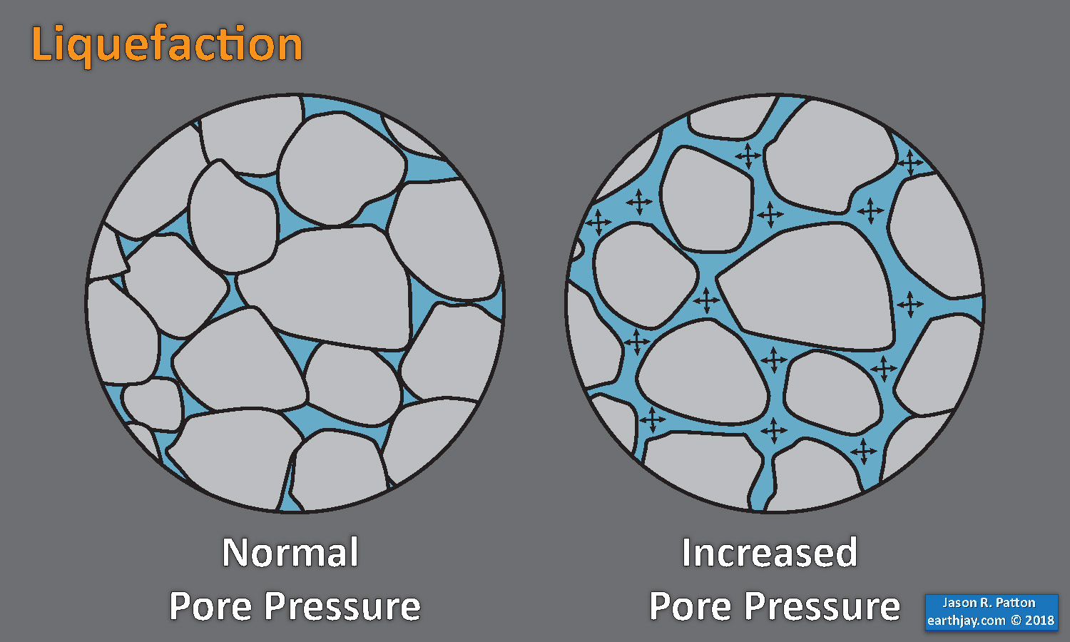
- Sediment or soil strength is based upon the ability for sediment particles to push against each other without moving. This is a combination of friction and the forces exerted between these particles. This is loosely what we call the “angle of internal friction.” Liquefaction is a process by which pore pressure increases cause water to push out against the sediment particles so that they are no longer touching.
- An analogy that some may be familiar with relates to a visit to the beach. When one is walking on the wet sand near the shoreline, the sand may hold the weight of our body generally pretty well. However, if we stop and vibrate our feet back and forth, this causes pore pressure to increase and we sink into the sand as the sand liquefies. Or, at least our feet sink into the sand.
- Below is a diagram showing how an increase in pore pressure can push against the sediment particles so that they are not touching any more. This allows the particles to move around and this is why our feet sink in the sand in the analogy above. This is also what changes the strength of earth materials such that a landslide can be triggered.
- Here Dr. Bohon demonstrates the phenomena of liquefaction.
- And, another video demonstration.
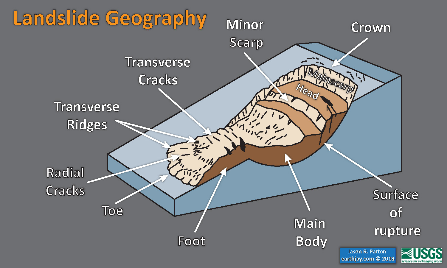
- Below is a diagram based upon a publication designed to educate the public about landslides and the processes that trigger them (USGS, 2004). Additional background information about landslide types can be found in Highland et al. (2008). There was a variety of landslide types that can be observed surrounding the earthquake region. So, this illustration can help people when they observing the landscape response to the earthquake whether they are using aerial imagery, photos in newspaper or website articles, or videos on social media. Will you be able to locate a landslide scarp or the toe of a landslide? This figure shows a rotational landslide, one where the land rotates along a curvilinear failure surface.
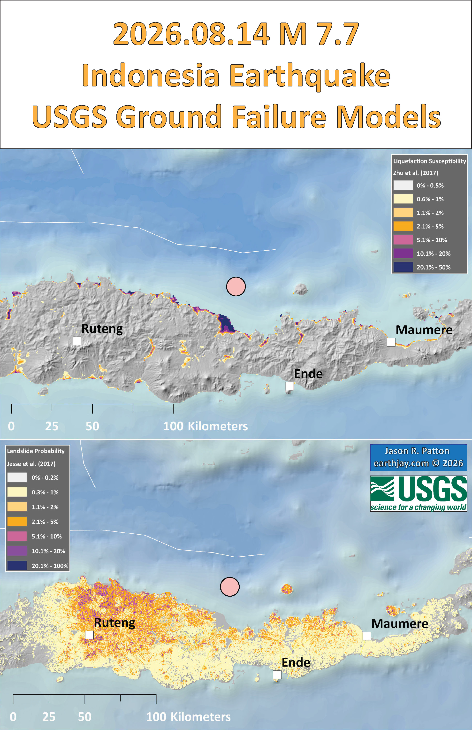
- Below is the liquefaction susceptibility and landslide probability map (Jessee et al., 2017; Zhu et al., 2017). Please head over to that report for more information about the USGS Ground Failure products (landslides and liquefaction). Basically, earthquakes shake the ground and this ground shaking can cause landslides.
- I use the same color scheme that the USGS uses on their website. Note how the areas that are more likely to have experienced earthquake induced liquefaction are in the valleys. Learn more about how the USGS prepares these model results here.
@drwendyrocksit #Liquefaction is a process by which water-saturated sediment temporarily loses strength and acts as a fluid. This can happen during #earthquake shaking. #geophysics #geology ♬ Quicksand – Hatchie
This liquefaction experiment conducted by the Tokyo Geological Survey of Japan at the Disaster Prevention Exhibition in 2015, shows the effects of different foundations and how hollow objects such as water pipes come to the surface [source, full video: https://t.co/xYLjPY4IHZ] pic.twitter.com/r8LXtmvrO0
— Massimo (@Rainmaker1973) April 17, 2021
Some Relevant Discussion and Figures
- Below is a map showing historic seismicity (Jones et al., 2014). Cross sections B-B’ and C-C’ are shown. The seismicity for the cross sections below are sourced from within each respective rectangle.
- Here are the seismcity cross sections.
- Below are the maps and cross sections from Darman et al., 2012.
- Here is the map in the interpretive poster above.
- Here is the seismicity cross section in the interpretive poster above.
- Here is their interpretations of seismic data used to interpret the tectonics of the subduction zone and Flores thrust.
- Here is the map from McCaffrey and Nabelek (1987). They used seismic reflection profiles, gravity modeling along these profiles, seismicity, and earthquake source mechanism analyses to support their interpretations of the structures in this region.
- Here is the Audley (2011) cross section showing how the backthrust relates to the subduction zone beneath Timor. I include their figure caption in blockquote below.
- This are the seismicity cross sections from Hangesh and Whitney (2016). These are shown to compare the subduction zone offshore of Java and the collision zone in the Timor region.
- Here is a map of the same general area from Silver et al. (1986), used here to locate the following large scale map.
- This is the large scale map showing the detailed thrust fault mapping (Silver et al., 1986).
- Here is the tectonic map from Hangesh and Whitney (2016).
- Here are some focal mechanisms from earthquakes in the region from Hangesh and Whitney (2016). Symbol color represents depth.
- This map from Hangesh and Whitney (2016) shows the GPS velocities in this region. Note the termination of the Flores thrust and the north-northeast striking (oriented) cross fault between Lombok and Sumbawa.
- Below are the 4 figures from Koulani et al., 2016. First is the plate tectonic map. I include their figure captions in block quote.
- This figure shows their estimates for plate motion relative velocities as derived from GPS data, constrained by the fault geometry in their block modeling.
- This figure shows their estimates of slip rate deficit along all the plate boundary faults in this region.
- Here is their figure that shows the slip deficit along the plate boundary faults.


Tectonic map of the Lesser Sunda Islands, showing the main tectonic units, main faults, bathymetry and location of seismic sections discussed in this paper.

This plot shows the earthquake localizations on a South-North cross section for the lat -14°/-4° long 114°/124° quadrant corresponding to the Lesser Sunda Islands region. The localizations are extracted from the USGS database and corresponds to magnitude greater than 4.5 in the 1973-2004 time period (shallow earthquakes with undetermined depth have been omitted.

Six 15 km deep seismic sections acquired by BGR from west to east traversing oceanic crust, deep sea trench, accretionary prism, outer arc high and fore-arc basin, derived from Kirchoff prestack depth migration (PreSDM) with a frequency range of 4-60 Hz. Profile BGR06-313 shows exemplarily a velocity-depth model according to refraction/wide-angle
seismic tomography on coincident profile P31 (modified after Lüschen et al, 2011).

Tectonic and geographic map of the eastern Sunda arc and vicinity. Active volcanoes are represented by triangles, and bathymetric contours are in kilometers. Thrust faults are shown with teeth on the upper plate. The dashed box encloses the study area.

Cartoon cross section of Timor today, (cf. Richardson & Blundell 1996, their BIRPS figs 3b, 4b & 7; and their fig. 6 gravity model 2 after Woodside et al. 1989; and Snyder et al. 1996 their fig. 6a). Dimensions of the filled 40 km deep present-day Timor Tectonic Collision Zone are based on BIRPS seismic, earthquake seismicity and gravity data all re-interpreted here from Richardson & Blundell (1996) and from Snyder et al. (1996). NB. The Bobonaro Melange, its broken formation and other facies are not indicated, but they are included with the Gondwana mega-sequence. Note defunct Banda Trench, now the Timor TCZ, filled with Australian continental crust and Asian nappes that occupy all space between Wetar Suture and the 2–3 km deep deformation front north of the axis of the Timor Trough. Note the much younger decollement D5 used exactly the same part of the Jurassic lithology of the Gondwana mega-sequence in the older D1 decollement that produced what appears to be much stronger deformation.

Comparison of hypocentral profiles across the (a) Java subduction zone and (b) Timor collision zone (paleo-Banda trench). Catalog compiled from multiple reporting agencies listed in Table 1. Events of Mw>4.0 are shown for period 1815 to 2015.

Location of SeaMARC II survey (Plate 1 and Figures 2) and geographic features discussed in text. Triangles on upper plates of thrust zones.
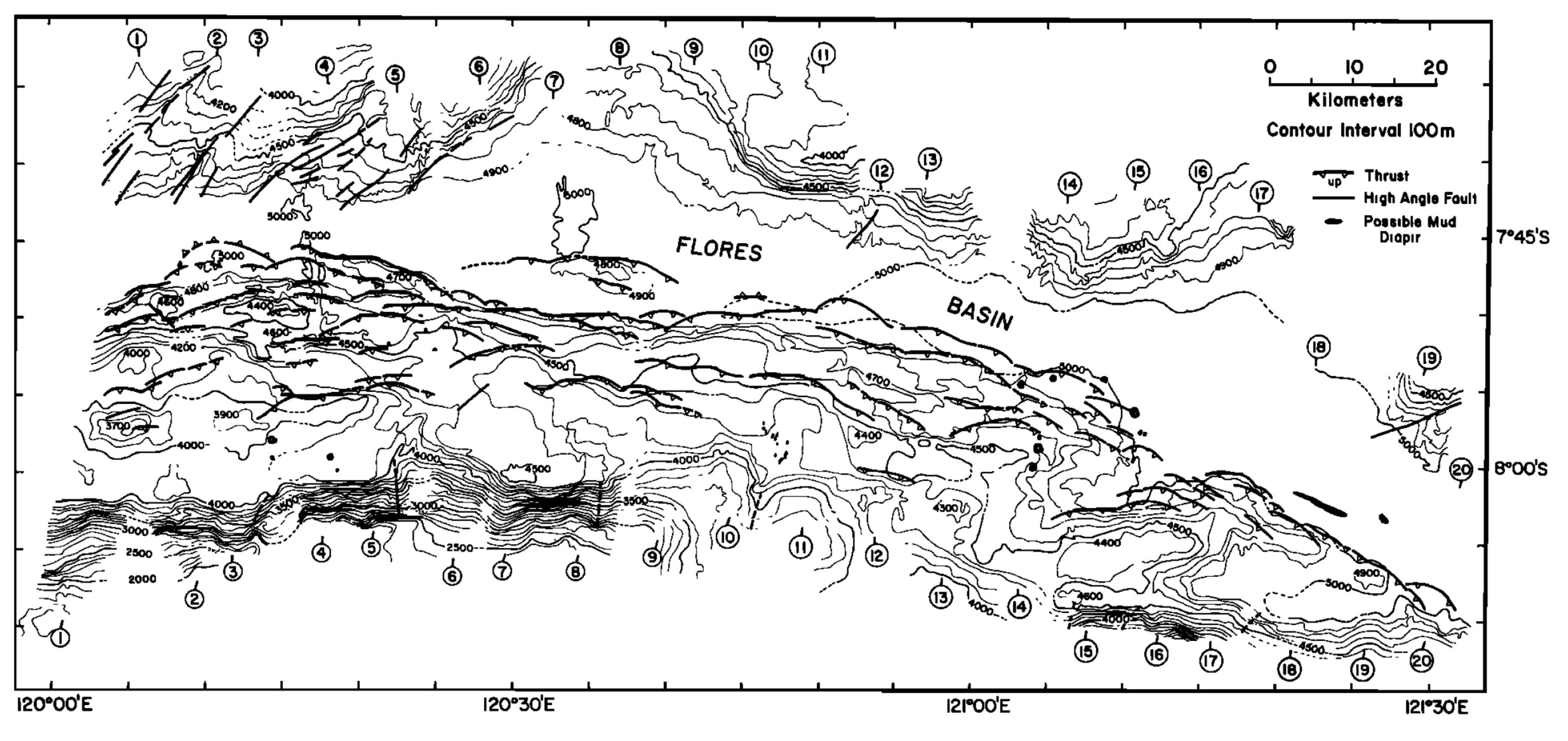
Bathymetry, faults, and mud diapirs of the central Flores thrust zone, based on interpretation of SeaMARC II data and seismic reflection profiles. Shown also are locations (circled numbers) of all seismic profiles. Mud diapirs are solid black. Triangles on upper plates of thrust faults.
Bathymetry, faults, and mud diapirs of the central Flores thrust zone, based on interpretation of SeaMARC II data and seismic reflection profiles. Shown also are locations (circled numbers) of all seismic profiles. Mud diapirs are solid black. Triangles on upper plates of thrust faults.

Illustration of major tectonic elements in triple junction geometry: tectonic features labeled per Figure 1; seismicity from ISC-GEM catalog [Storchak et al., 2013]; faults in Savu basin from Rigg and Hall [2011] and Harris et al. [2009]. Purple line is edge of Australian continental basement and fore arc [Rigg and Hall, 2011]. Abbreviations: AR = Ashmore Reef; SR = Scott Reef; RS = Rowley Shoals; TCZ = Timor Collision Zone; ST = Savu thrust; SB = Savu Basin; TT = Timor thrust; WT =Wetar thrust; WASZ = Western Australia Shear Zone. Open arrows indicate relative direction of motion; solid arrows direction of vergence.

(a) Focal mechanism solutions for the study region. The focal mechanisms are classified based on depth intervals to illustrate the style of faulting within the different structural domains. Note (b) sinistral reverse motion along Timor trough, (c) subduction related pattern along Java trench, and dextral solutions along the western Australia extended margin (Figure 4a) north of 20°S. Centroid moment tensor (CMT) solutions [Dziewonski et al., 1981] are from the CMT project [Ekström et al., 2012; http://www.globalcmt.org/CMTcite.html] for events of Mw>5.0 for the period 1976 onward.

GPS velocities of Sunda and Banda arc region. Large black and grey arrow shows motion of Australia relative to Eurasia [DeMets et al., 1994]. Thin black arrows show GPS velocities of Sunda and Banda arc regions relative to Australia [Nugroho et al., 2009]. Seismicity from ISC-GEM catalog [Storchak et al., 2013]. Note reduction of station velocities from west to east indicating progressive coupling of the Banda arc to the Australian plate compared to the area along the Sunda arc.

Seismotectonic setting of the Sunda-Banda arc-continent collision, East Indonesia. Major faults (thick black lines) [Hamilton, 1979]. Topography and bathymetry are from Shuttle Radar Topography Mission (http://topex.ucsd.edu/www_html/srtm30_plus.html). Focal mechanisms are from the Global Centroid Moment Tensor. Blue mechanisms correspond to earthquakes with Mw>7 (brown transparent ellipses are the corresponding rupture areas for Flores 1992 and Alor 2004 earthquakes), while the green focal mechanism shows the highest magnitude recorded in Sumbawa. Red dots indicate the locations of major historical earthquakes [Musson, 2012].

GPS velocities determined in this study with respect to Sunda Block. Uncertainty ellipses represent 95% confidence level. The inset figure corresponds to the area of the dashed rectangle in the map. Light blue arrows show the velocities for East and West Makassar Blocks.

Relative slip vectors across block boundaries, derived from our best fit model. Arrows show motion of the hanging wall (moving block) relative to the footwall (fixed block) with 95% confidence ellipses. The tails of arrows is located within the “moving” block. Black thick lines show well-defined boundaries we use as active faults in our model and dashed lines show less well-defined boundaries (green : free-slipping boundaries and black: fixed locked faults) . Principal axes of the horizontal strain tensor estimated for the SUMB, EMAK, and EJAV are shown in pink. The thick pink arrow shows the relative motion of Australia with respect to Sunda (AUST/SUND). Abbreviations are Sumba Block (SUMB), West Makassar Block (WMAK), East Makassar Block (EMAK), East Java Block (EJAV), and Timor Block (TIMO). The background seismicity is from the International Seismological Centre catalog with magnitudes ≥5.5 and depths <40 km.

Fault slip rate components: (a) fault normal (extension positive) and (b) fault parallel (right-lateral positive).
Seismic Hazard and Seismic Risk
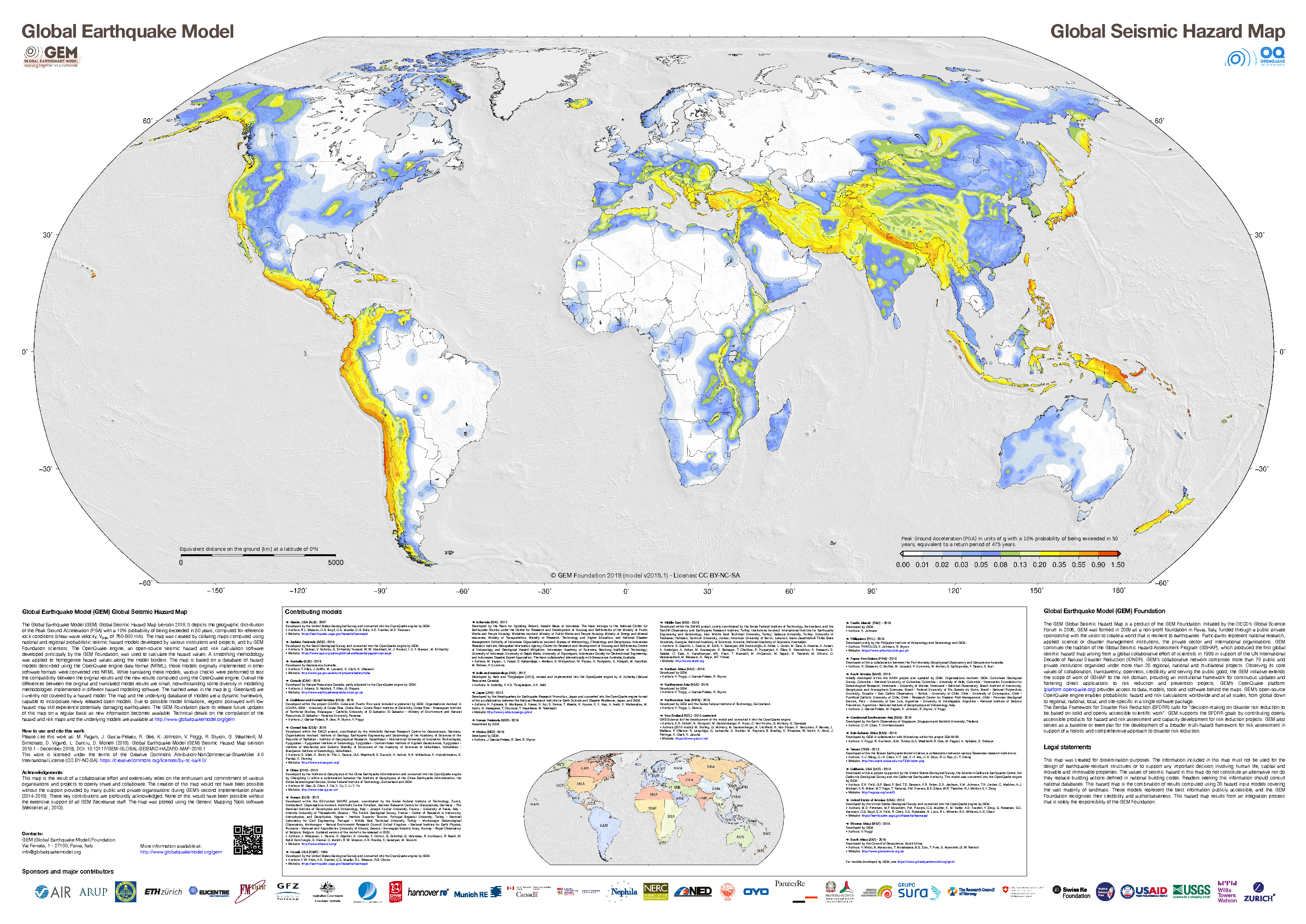
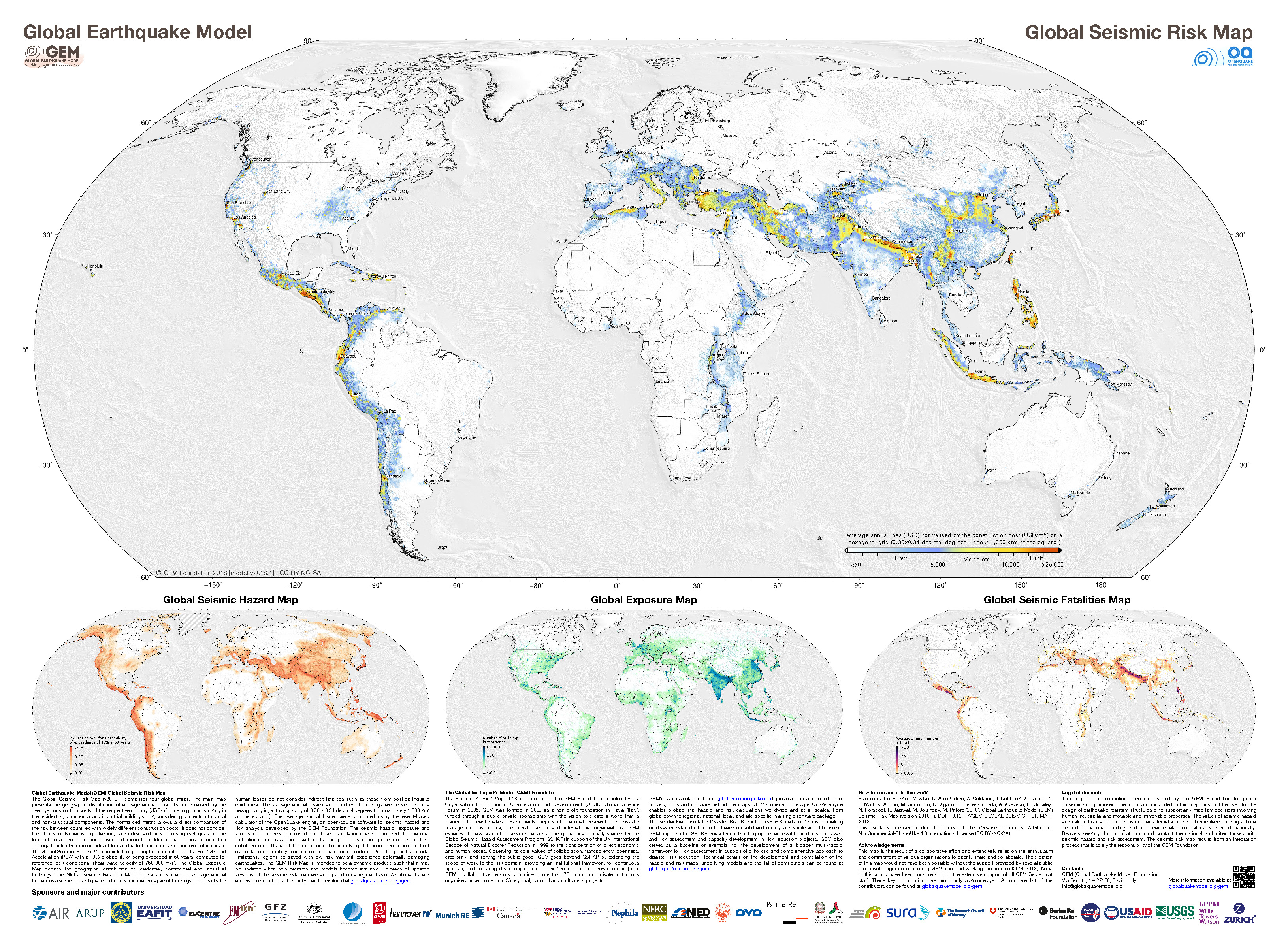
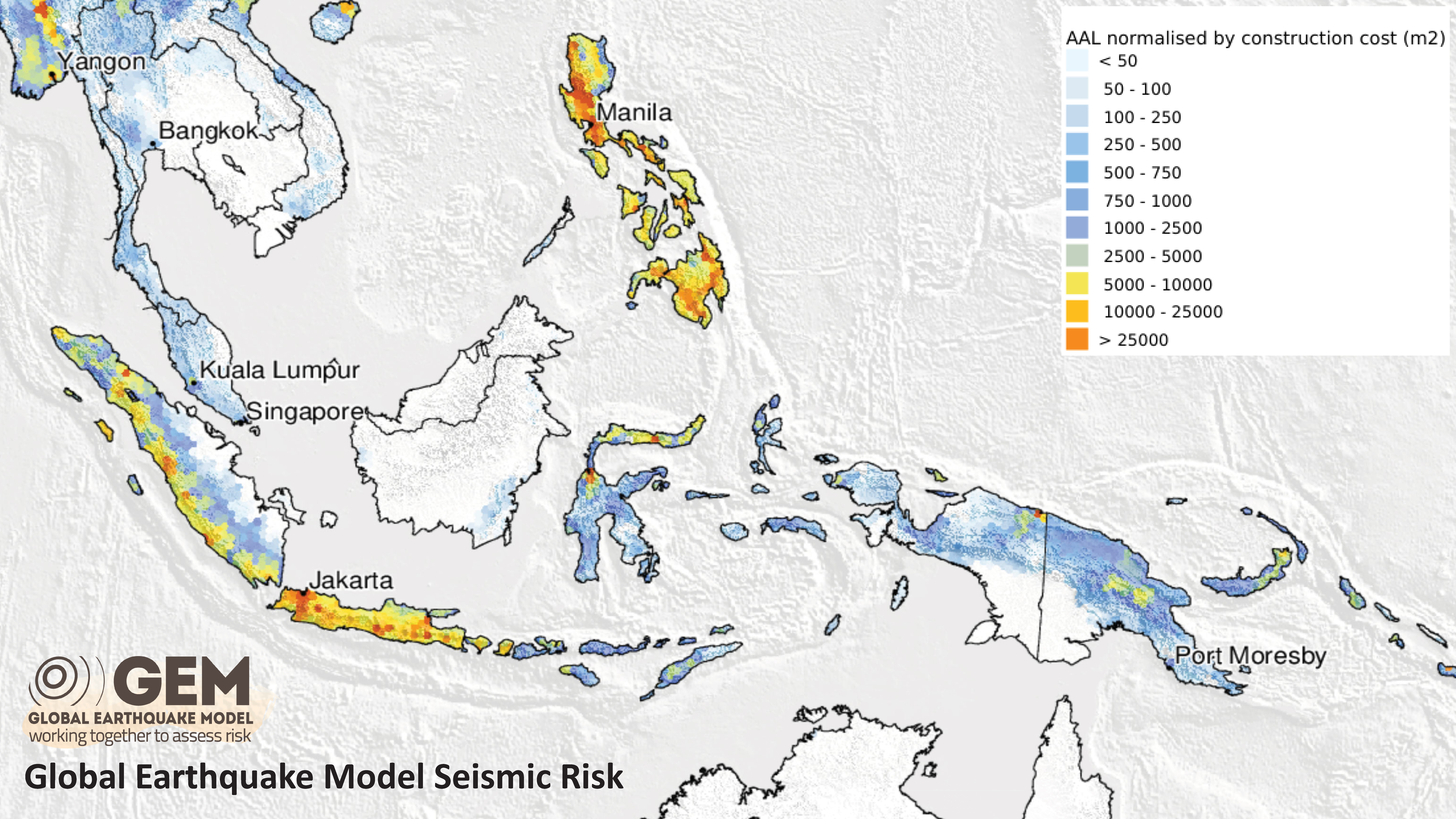
- These are the two maps shown in the map above, the GEM Seismic Hazard and the GEM Seismic Risk maps from Pagani et al. (2018) and Silva et al. (2018).
- The GEM Seismic Hazard Map:
- The Global Earthquake Model (GEM) Global Seismic Hazard Map (version 2018.1) depicts the geographic distribution of the Peak Ground Acceleration (PGA) with a 10% probability of being exceeded in 50 years, computed for reference rock conditions (shear wave velocity, VS30, of 760-800 m/s). The map was created by collating maps computed using national and regional probabilistic seismic hazard models developed by various institutions and projects, and by GEM Foundation scientists. The OpenQuake engine, an open-source seismic hazard and risk calculation software developed principally by the GEM Foundation, was used to calculate the hazard values. A smoothing methodology was applied to homogenise hazard values along the model borders. The map is based on a database of hazard models described using the OpenQuake engine data format (NRML). Due to possible model limitations, regions portrayed with low hazard may still experience potentially damaging earthquakes.
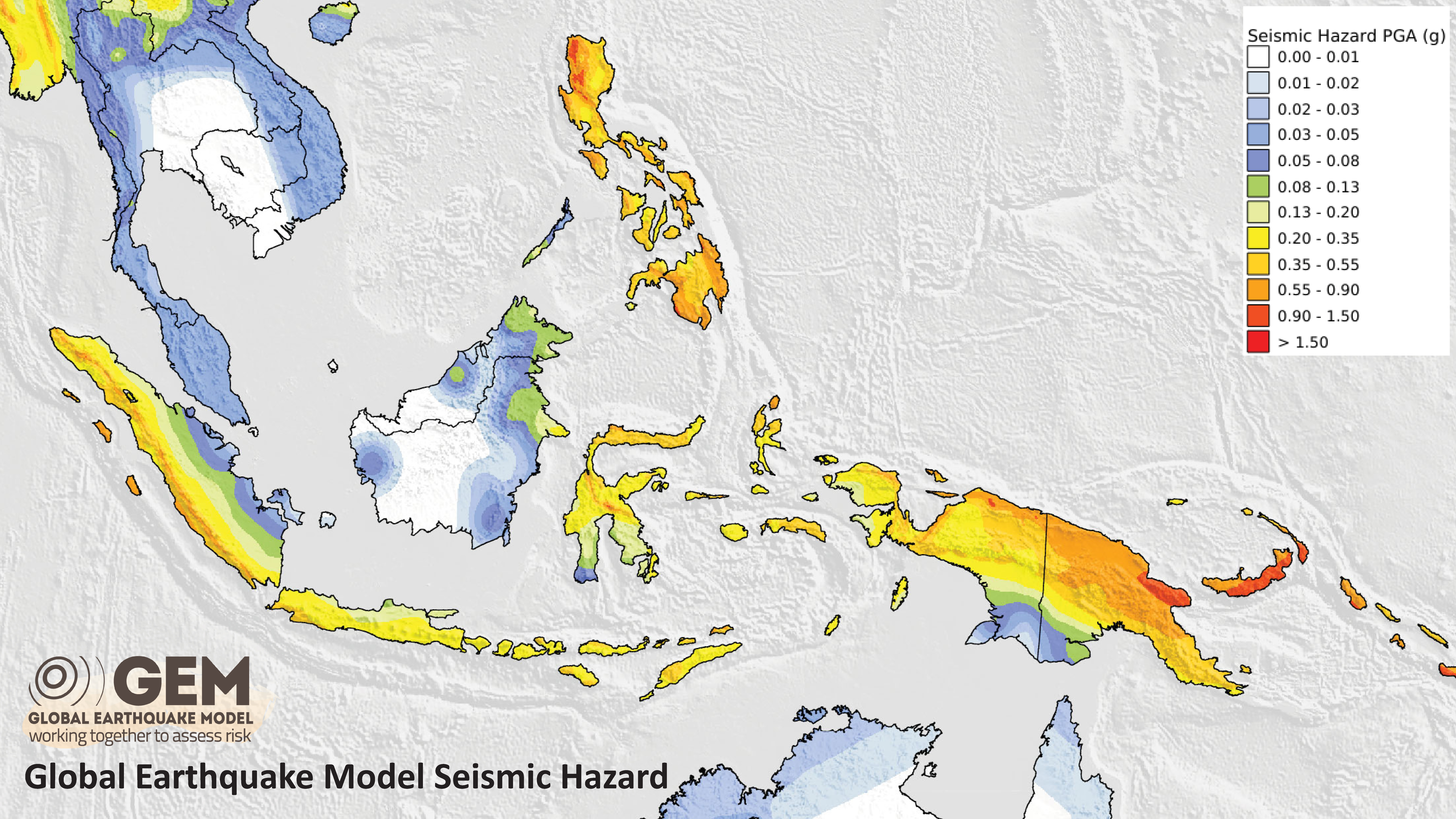
- Here is a view of the GEM seismic hazard map for Indonesia.
- The USGS Seismic Hazard Map:
- Here is another version of the seismic hazard for this region (Smoczyk et al., 2013). The GEM map suggests that the islands along the Halmahera Strait may have accelerations between 0.8-1.6 m2. This translates to 0.08 to 0.16 g. The GEM seismic hazard map shows a potential shaking of 0.20-0.35 g, slightly higher.
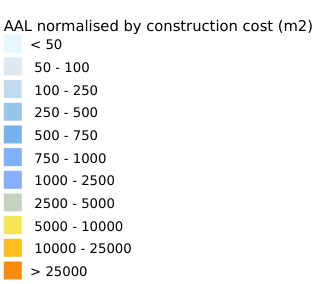
- The GEM Seismic Risk Map:
- The Global Seismic Risk Map (v2018.1) presents the geographic distribution of average annual loss (USD) normalised by the average construction costs of the respective country (USD/m2) due to ground shaking in the residential, commercial and industrial building stock, considering contents, structural and non-structural components. The normalised metric allows a direct comparison of the risk between countries with widely different construction costs. It does not consider the effects of tsunamis, liquefaction, landslides, and fires following earthquakes. The loss estimates are from direct physical damage to buildings due to shaking, and thus damage to infrastructure or indirect losses due to business interruption are not included. The average annual losses are presented on a hexagonal grid, with a spacing of 0.30 x 0.34 decimal degrees (approximately 1,000 km2 at the equator). The average annual losses were computed using the event-based calculator of the OpenQuake engine, an open-source software for seismic hazard and risk analysis developed by the GEM Foundation. The seismic hazard, exposure and vulnerability models employed in these calculations were provided by national institutions, or developed within the scope of regional programs or bilateral collaborations.


Tsunami Hazard
- Here are two maps that show the results of probabilistic tsunami modeling for the nation of Indonesia (Horspool et al., 2014). These results are similar to results from seismic hazards analysis and maps. The color represents the chance that a given area will experience a certain size tsunami (or larger).
- The first map shows the annual chance of a tsunami with a height of at least 0.5 m (1.5 feet). The second map shows the chance that there will be a tsunami at least 3 meters (10 feet) high at the coast.
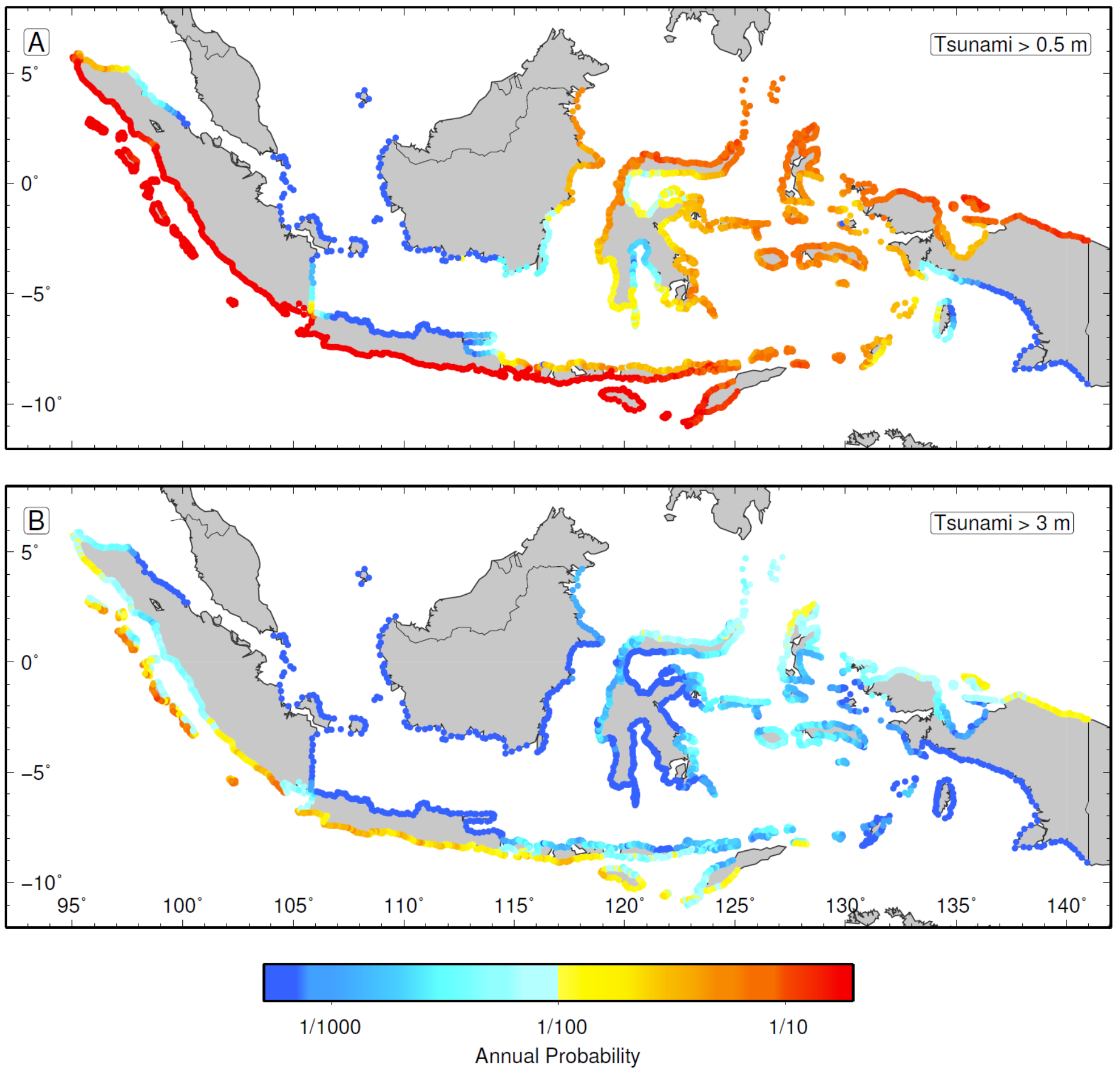
Annual probability of experiencing a tsunami with a height at the coast of (a) 0.5m (a tsunami warning) and (b) 3m (a major tsunami warning).
- M 9.2 Andaman-Sumatra subduction zone 2014 Earthquake Anniversary
- M 9.2 Andaman-Sumatra subduction zone SASZ Fault Deformation
- M 9.2 Andaman-Sumatra subduction zone 2016 Earthquake Anniversary
- 2026.08.14 M 7.7 Indonesia (Flores Isle) 350
- 2023.11.08 M 7.1 Banda Sea
- 2023.08.28 M 7.1 Lombok & Bali, Indonesia
- 2023.04.24 M 7.1 Sumatra
- 2022.11.18 M 6.9 Sumatra
- 2022.02.25 M 6.2 Sumatra
- 2020.05.06 M 6.8 Banda Sea
- 2019.08.02 M 6.9 Indonesia
- 2019.06.23 M 7.3 Banda Sea
- 2019.04.12 M 6.8 Sulawesi, Indonesia
- 2018.09.28 M 7.5 Sulawesi
- 2018.10.16 M 7.5 Sulawesi UPDATE #1
- 2018.08.19 M 6.9 Lombok, Indonesia
- 2018.08.05 M 6.9 Lombok, Indonesia
- 2018.07.28 M 6.4 Lombok, Indonesia
- 2017.12.15 M 6.5 Java
- 2017.08.31 M 6.3 Mentawai, Sumatra
- 2017.08.13 M 6.4 Bengkulu, Sumatra, Indonesia
- 2017.05.29 M 6.8 Sulawesi, Indonesia
- 2017.03.14 M 6.0 Sumatra
- 2017.03.01 M 5.5 Banda Sea
- 2016.10.19 M 6.6 Java
- 2016.03.02 M 7.8 Sumatra/Indian Ocean
- 2015.07.22 M 5.8 Andaman Sea
- 2015.11.08 M 6.4 Nicobar Isles
- 2012.04.11 M 8.6 Sumatra outer rise
- 2004.12.26 M 9.2 Andaman-Sumatra subduction zone
Indonesia | Sumatra
General Overview
Earthquake Reports
Social Media
My thread:
#EarthquakeReport for M 7.7 #Gempa #Earthquake offshore of Timor #Indonesia
Reverse (compressional) earthquake mechanism
Appears related to Flores backthrust fault
Hopefully few casualties
Tectonic setting in 2019 report https://t.co/i5eSZKqY8Yhttps://t.co/NvQMfmYk1P pic.twitter.com/WKwr0nQgVB
— Jason "Jay" R. Patton (@patton_cascadia) August 14, 2026
- Frisch, W., Meschede, M., Blakey, R., 2011. Plate Tectonics, Springer-Verlag, London, 213 pp.
- Hayes, G., 2018, Slab2 – A Comprehensive Subduction Zone Geometry Model: U.S. Geological Survey data release, https://doi.org/10.5066/F7PV6JNV.
- Holt, W. E., C. Kreemer, A. J. Haines, L. Estey, C. Meertens, G. Blewitt, and D. Lavallee (2005), Project helps constrain continental dynamics and seismic hazards, Eos Trans. AGU, 86(41), 383–387, , https://doi.org/10.1029/2005EO410002. /li>
- Jessee, M.A.N., Hamburger, M. W., Allstadt, K., Wald, D. J., Robeson, S. M., Tanyas, H., et al. (2018). A global empirical model for near-real-time assessment of seismically induced landslides. Journal of Geophysical Research: Earth Surface, 123, 1835–1859. https://doi.org/10.1029/2017JF004494
- Kreemer, C., J. Haines, W. Holt, G. Blewitt, and D. Lavallee (2000), On the determination of a global strain rate model, Geophys. J. Int., 52(10), 765–770.
- Kreemer, C., W. E. Holt, and A. J. Haines (2003), An integrated global model of present-day plate motions and plate boundary deformation, Geophys. J. Int., 154(1), 8–34, , https://doi.org/10.1046/j.1365-246X.2003.01917.x.
- Kreemer, C., G. Blewitt, E.C. Klein, 2014. A geodetic plate motion and Global Strain Rate Model in Geochemistry, Geophysics, Geosystems, v. 15, p. 3849-3889, https://doi.org/10.1002/2014GC005407.
- Meyer, B., Saltus, R., Chulliat, a., 2017. EMAG2: Earth Magnetic Anomaly Grid (2-arc-minute resolution) Version 3. National Centers for Environmental Information, NOAA. Model. https://doi.org/10.7289/V5H70CVX
- Müller, R.D., Sdrolias, M., Gaina, C. and Roest, W.R., 2008, Age spreading rates and spreading asymmetry of the world’s ocean crust in Geochemistry, Geophysics, Geosystems, 9, Q04006, https://doi.org/10.1029/2007GC001743
- Pagani,M. , J. Garcia-Pelaez, R. Gee, K. Johnson, V. Poggi, R. Styron, G. Weatherill, M. Simionato, D. Viganò, L. Danciu, D. Monelli (2018). Global Earthquake Model (GEM) Seismic Hazard Map (version 2018.1 – December 2018), DOI: 10.13117/GEM-GLOBAL-SEISMIC-HAZARD-MAP-2018.1
- Silva, V ., D Amo-Oduro, A Calderon, J Dabbeek, V Despotaki, L Martins, A Rao, M Simionato, D Viganò, C Yepes, A Acevedo, N Horspool, H Crowley, K Jaiswal, M Journeay, M Pittore, 2018. Global Earthquake Model (GEM) Seismic Risk Map (version 2018.1). https://doi.org/10.13117/GEM-GLOBAL-SEISMIC-RISK-MAP-2018.1
- Storchak, D. A., D. Di Giacomo, I. Bondár, E. R. Engdahl, J. Harris, W. H. K. Lee, A. Villaseñor, and P. Bormann (2013), Public release of the ISC-GEM global instrumental earthquake catalogue (1900–2009), Seismol. Res. Lett., 84(5), 810–815, doi:10.1785/0220130034.
- Zhu, J., Baise, L. G., Thompson, E. M., 2017, An Updated Geospatial Liquefaction Model for Global Application, Bulletin of the Seismological Society of America, 107, p 1365-1385, https://doi.org/0.1785/0120160198
- Audley-Charles, M.G., 1986. Rates of Neogene and Quaternary tectonic movements in the Southern Banda Arc based on micropalaeontology in: Journal of fhe Geological Society, London, Vol. 143, 1986, pp. 161-175.
- Audley-Charles, M.G., 2011. Tectonic post-collision processes in Timor, Hall, R., Cottam, M. A. &Wilson, M. E. J. (eds) The SE Asian Gateway: History and Tectonics of the Australia–Asia Collision. Geological Society, London, Special Publications, 355, 241–266.
- Baldwin, S.L., Fitzgerald, P.G., and Webb, L.E., 2012. Tectonics of the New Guinea Region in Annu. Rev. Earth Planet. Sci., v. 41, p. 485-520.
- Benz, H.M., Herman, Matthew, Tarr, A.C., Hayes, G.P., Furlong, K.P., Villaseñor, Antonio, Dart, R.L., and Rhea, Susan, 2011. Seismicity of the Earth 1900–2010 New Guinea and vicinity: U.S. Geological Survey Open-File Report 2010–1083-H, scale 1:8,000,000.
- Given, J. W., and H. Kanamori (1980). The depth extent of the 1977 Sumbawa, Indonesia, earthquake, in EOS Trans. AGU., v. 61, p. 1044.
- Gusnman, A.R., Tanioka, Y., Matsumoto, H., and Iwasakai, S.-I., 2009. Analysis of the Tsunami Generated by the Great 1977 Sumba Earthquake that Occurred in Indonesia in BSSA, v. 99, no. 4, p. 2169-2179, https://doi.org/10.1785/0120080324
- Hall, R., 2011. Australia-SE Asia collision: plate tectonics and crustal flow in Geological Society, London, Special Publications 2011; v. 355; p. 75-109 doi: 10.1144/SP355.5
- Hangesh, J. and Whitney, B., 2014. Quaternary Reactivation of Australia’s Western Passive Margin: Inception of a New Plate Boundary? in: 5th International INQUA Meeting on Paleoseismology, Active Tectonics and Archeoseismology (PATA), 21-27 September 2014, Busan, Korea, 4 pp.
- Koulali, A., S. Susilo, S. McClusky, I. Meilano, P. Cummins, P. Tregoning, G. Lister, J. Efendi, and M. A. Syafi’i, 2016. Crustal strain partitioning and the associated earthquake hazard in the eastern Sunda-Banda Arc in Geophys. Res. Lett., 43, 1943–1949, doi:10.1002/2016GL067941
- Okal, E. A., & Reymond, D., 2003. The mechanism of great Banda Sea earthquake of 1 February 1938: applying the method of preliminary determination of focal mechanism to a historical event in EPSL, v. 216, p. 1-15.
- Osada, M. and Abe, K., 1981. Mechanism and tectonic implications of the great Banda Sea earthquake of November 4, 1963 in Physics of the Earth and Plentary Interiors, v. 25, p. 129-139
- Pownall, J.M., Hall, R., Armstrong,, R.A., and Forster, M.A., 2014. Earth’s youngest known ultrahigh-temperature granulites discovered on Seram, eastern Indonesia in Geology, v. 42, no. 4, p. 379-282, https://doi.org/10.1130/G35230.1
- Spakman, W. and Hall, R., 2010. Surface deformation and slab–mantle interaction during Banda arc subduction rollback in Nature Geosceince, v. 3, p. 562-566, https://doi.org/10.1038/NGEO917
- Whitney, B.B. and Hengesh, J.V., 2015. A new model for active intraplate tectonics in western Australia in Proceedings of the Tenth Pacific Conference on Earthquake Engineering Building an Earthquake-Resilient Pacific 6-8 November 2015, Sydney, Australia, paper number 82
- Zahirovic, S., Seton, M., and Müller, R.D., 2014. The Cretaceous and Cenozoic tectonic evolution of Southeast Asia in Solid Earth, v. 5, p. 227-273, doi:10.5194/se-5-227-2014
References:
Basic & General References
Specific References
Return to the Earthquake Reports page.
- Sorted by Magnitude
- Sorted by Year
- Sorted by Day of the Year
- Sorted By Region