This morning (my time) there was a moderately deep earthquake along the coast of southern Mexico and northern Guatemala. Here is my Temblor article about this M=6.6 earthquake and how it might relate to the 2017 M=8.2 quake.
https://earthquake.usgs.gov/earthquakes/eventpage/us2000jbub/executive
Offshore of Guatemala and Mexico, the Middle America trench is formed by the subduction of the oceanic Cocos plate beneath the North America and Caribbean plates.
To the east of Guatemala and Mexico, the North America and Caribbean plates are separated by a left lateral (sinistral) strike-slip plate boundary fault (that forms the Cayman Trough beneath the Caribbean Sea).
As this plate boundary comes onshore, this fault forms multiple splays, including the Polochi-Montagua fault. As this system trends westwards across Central America, it joins another strike-slip plate boundary associated with the subduction zone (the Volcanic Arc fault).
South of about 15°N, the relative plate motion between the Caribbean and Cocos plates is oblique (they are not moving towards each other in a direction perpendicular to the subduction zone fault). At plate boundaries where plate convergence is oblique (like also found in Sumatra), the strain is partitioned onto the subduction zone (for fault normal component of the relative plate motion) and a forearc sliver fault (for the fault parallel relative motion).
The Tehuantepec fracture zone (TFZ) is a major structure in the Cocos plate. Coincidentally, the strike-slip fault systems trend towards where the TFZ intersects the trench.
There is left-lateral offset of the seafloor across the TFZ so the crust is about 10 million years older on the north side of the eastern TFZ. This age offset changes the depth of the crust across the TFZ and also may affect the megathrust fault properties on either side of the TFZ.
In addition, the TFZ may have geological properties that also affect the fault properties when this part of the plate subducts (affecting where, when, and how the fault slips).
There are so many things going on, but I will mention one more thing. Something that also appears to be happening in this part of the subduction zone is that there may be gaps in the slab beneath the megathrust. If this is true (Mann, 2007), then there may be changes in slab pull tension along strike as a result of different widths of attached downgoing slab.
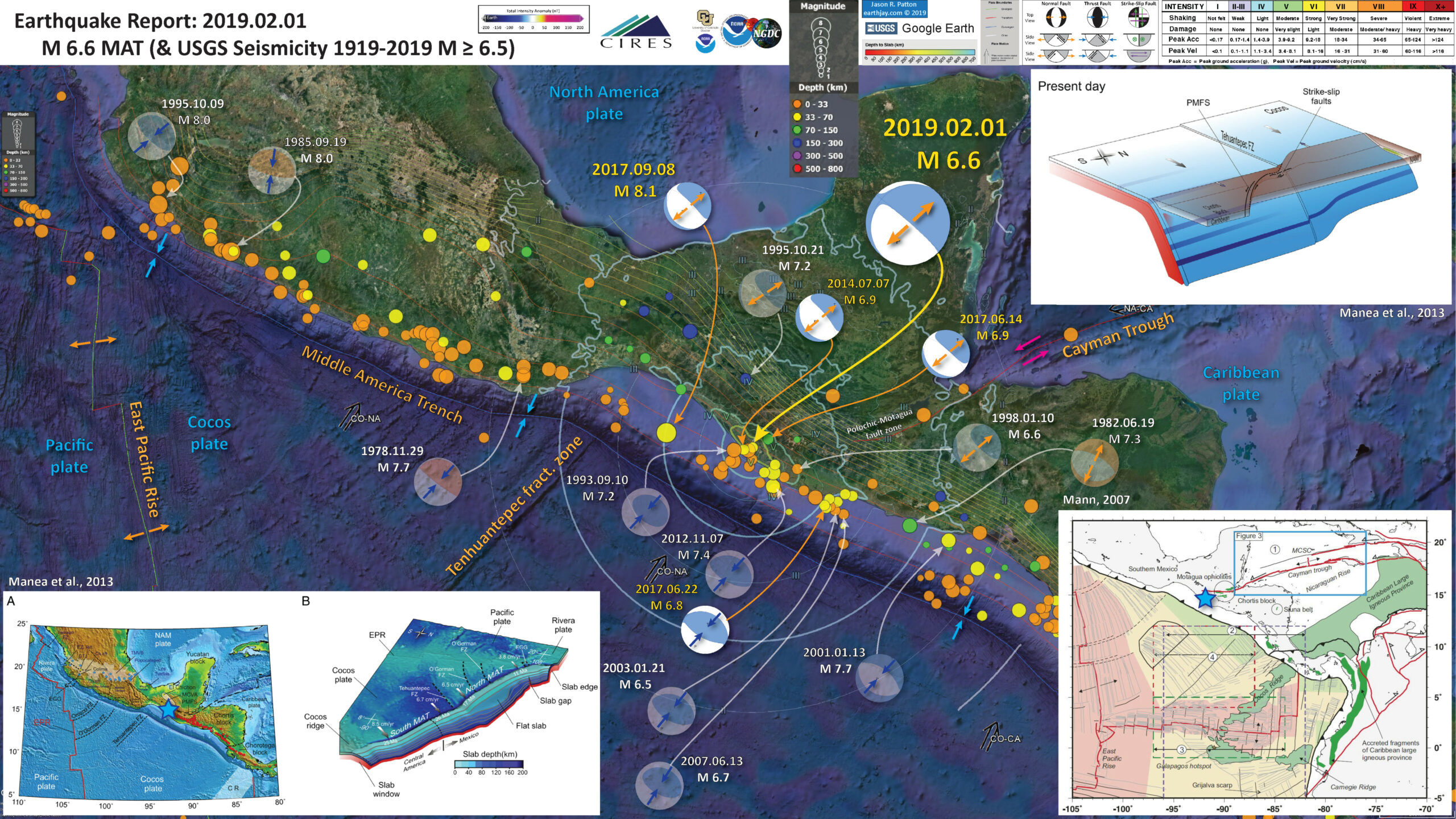
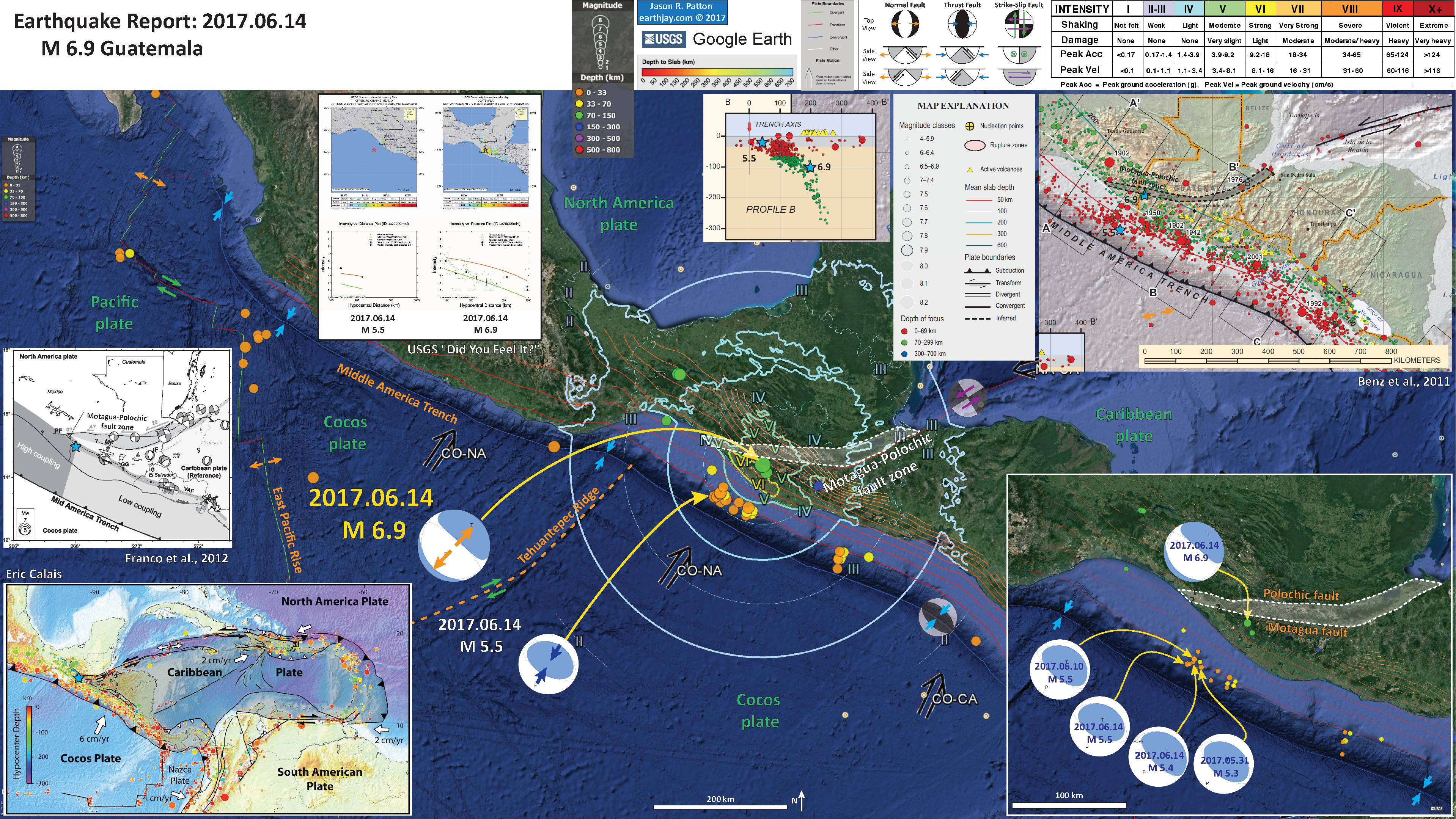
Below is my interpretive poster for this earthquake
I plot the seismicity from the past month, with color representing depth and diameter representing magnitude (see legend). I include earthquake epicenters from 1919-2019 with magnitudes M ≥ 6.5 in one version.
I plot the USGS fault plane solutions (moment tensors in blue and focal mechanisms in orange), possibly in addition to some relevant historic earthquakes.
- I placed a moment tensor / focal mechanism legend on the poster. There is more material from the USGS web sites about moment tensors and focal mechanisms (the beach ball symbols). Both moment tensors and focal mechanisms are solutions to seismologic data that reveal two possible interpretations for fault orientation and sense of motion. One must use other information, like the regional tectonics, to interpret which of the two possibilities is more likely.
- I also include the shaking intensity contours on the map. These use the Modified Mercalli Intensity Scale (MMI; see the legend on the map). This is based upon a computer model estimate of ground motions, different from the “Did You Feel It?” estimate of ground motions that is actually based on real observations. The MMI is a qualitative measure of shaking intensity. More on the MMI scale can be found here and here. This is based upon a computer model estimate of ground motions, different from the “Did You Feel It?” estimate of ground motions that is actually based on real observations.
- I include a transparent version of the slab 2.0 contours plotted (Hayes, 2018), which are contours that represent the depth to the subduction zone fault. These are mostly based upon seismicity. The depths of the earthquakes have considerable error and do not all occur along the subduction zone faults, so these slab contours are simply the best estimate for the location of the fault.li>
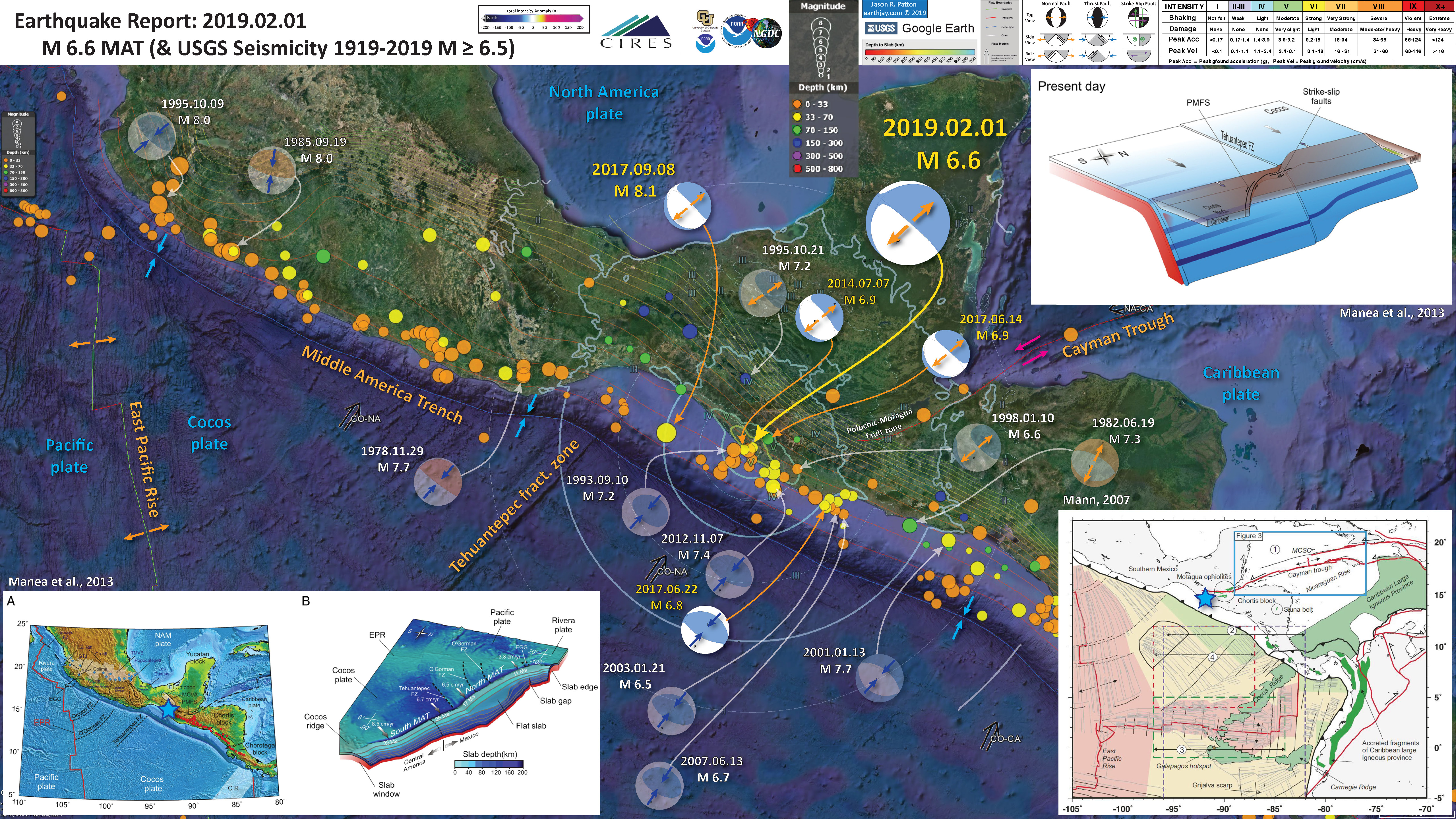
- In the map below, I include a transparent overlay of the magnetic anomaly data from EMAG2 (Meyer et al., 2017). As oceanic crust is formed, it inherits the magnetic field at the time. At different points through time, the magnetic polarity (north vs. south) flips, the north pole becomes the south pole. These changes in polarity can be seen when measuring the magnetic field above oceanic plates. This is one of the fundamental evidences for plate spreading at oceanic spreading ridges (like the Gorda rise).
- Regions with magnetic fields aligned like today’s magnetic polarity are colored red in the EMAG2 data, while reversed polarity regions are colored blue. Regions of intermediate magnetic field are colored light purple.
Magnetic Anomalies
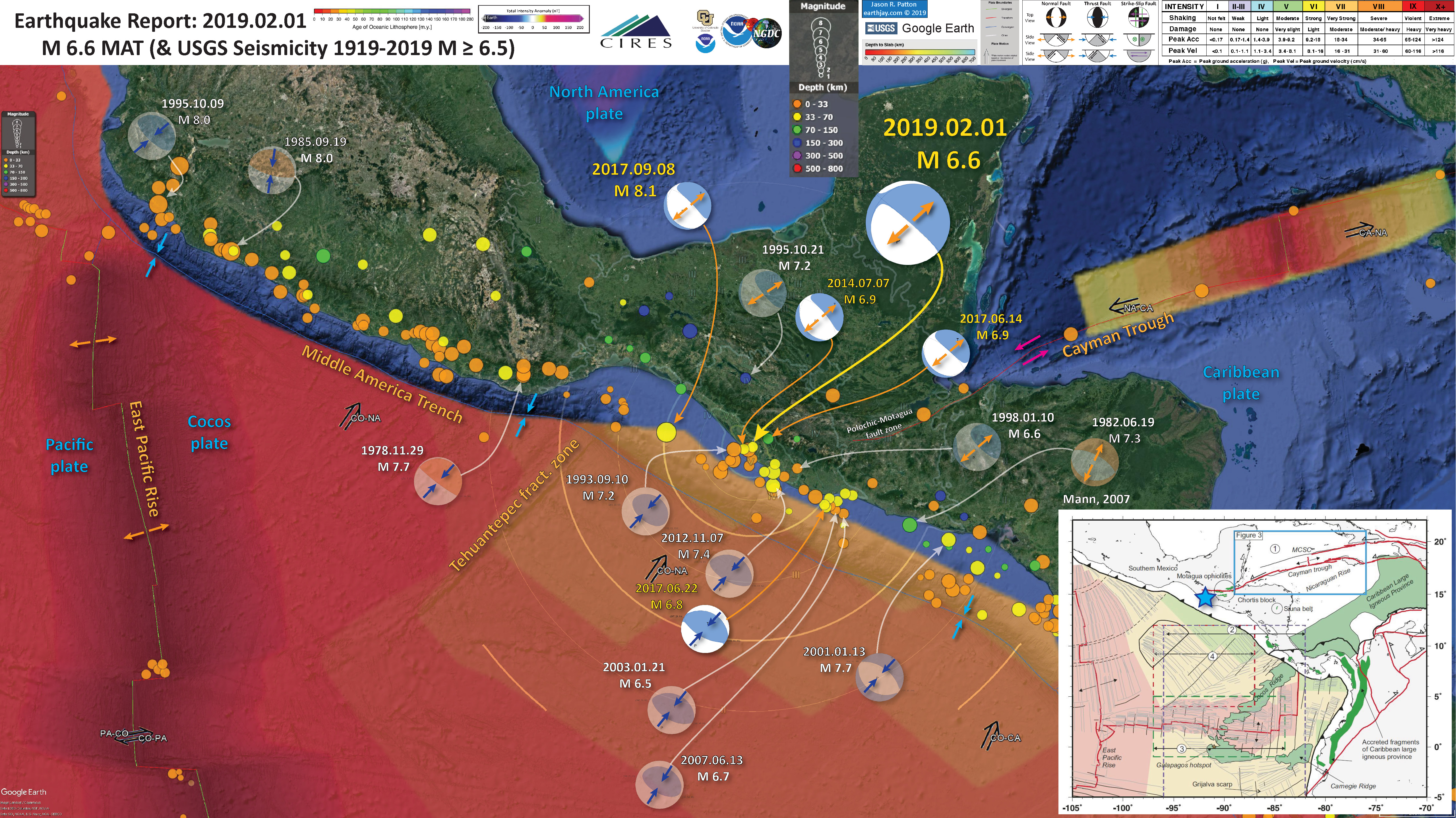
- In one map below, I include a transparent overlay of the age of the oceanic crust data from Agegrid V 3 (Müller et al., 2008).
- Because oceanic crust is formed at oceanic spreading ridges, the age of oceanic crust is youngest at these spreading ridges. The youngest crust is red and older crust is yellow (see legend at the top of this poster).
Age of Oceanic Lithosphere
- In the lower left corner is a pair of figures from Manea et al. (2013). On the left is a map showing some major plate boundary faults and other fault systems relevant to this region. On the right is a low angle oblique visualization of the Cocos plate. North is to the lower right. The depth of the slab is shown in shades of blue (see legend). Note the offset of blue color across the TFZ.
- In the upper right corner is another low angle oblique visualization of the structures (Manea et al., 2013). Note the difference in depth of the slab across the TFZ and how the forearc sliver and North America / Caribbean strike-slip faults cross the upper plate. Read more about the forearc sliver in this report about an earthquake in El Salvador.
- In the lower right corner is a map of the region showing details of the structures in the Cocos plate (Mann, 2007). There are an abundance of faults associated with the spreading ridges and offsets of these by numerous fracture zones. Note how the Cocos plate is formed by 2 different spreading ridges.
I include some inset figures. Some of the same figures are located in different places on the larger scale map below.
- Here is the map with a century’s seismicity plotted.
- Here is the map with a century’s seismicity plotted, using the age of the crust as an overlay.
There are also some interesting relations between different historic earthquakes.
In 2017 there was a series of large magnitude earthquakes in the region of today’s M=6.6 and further to the south. These quakes are highlighted in the posters above, notable are the 6 Jun M=6.9 and 22 Jun M=6.8. The first quake was a deep extensional event, followed by a thrust event (possibly triggered by the M=6.9). In addition, there was a M=6.9 extensional earthquake in 2014 that also may have been a player.
I presented an interpretive poster showing the zone of aftershocks associated with the June sequence. Later, in Sept, there was a M=8.2 extensional tsunamigenic earthquake to the north of the June sequence. If we look at the aftershock zone for the M=8.2 quake, it looks like a sausage link adjacent to the sausage link formed by the June aftershocks. mmmm veggie sausages.
However there was no megathrust earthquake in the area of the M=8.2 sequence.
- Here is an interpretive poster showing how the 2017 June and September sequences spatially relate.
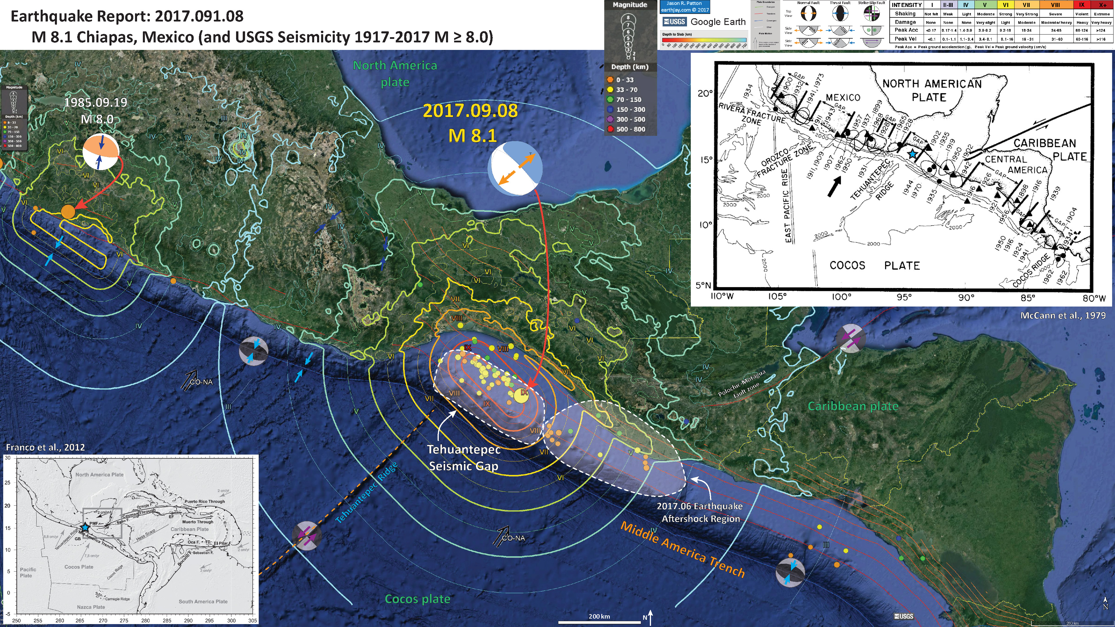
- Here is a report where I discuss the June 2017 sequence in greater detail.
Other Report Pages
Some Relevant Discussion and Figures
- Here are some figures from Manea et al. (2013). First are the map and low angle oblique view of the Cocos plate.
- Here is the figure that shows how the upper and lower plate structures interplay.

A. Geodynamic and tectonic setting alongMiddle America Subduction Zone. JB: Jalisco Block; Ch. Rift—Chapala rift; Co. rift—Colima rift; EGG—El Gordo Graben; EPR: East Pacific Rise; MCVA: Modern Chiapanecan Volcanic Arc; PMFS: Polochic–Motagua Fault System; CR—Cocos Ridge. Themain Quaternary volcanic centers of the TransMexican Volcanic Belt (TMVB) and the Central American Volcanic Arc (CAVA) are shown as blue and red dots, respectively. B. 3-D view of the Pacific, Rivera and Cocos plates’ bathymetrywith geometry of the subducted slab and contours of the depth to theWadati–Benioff zone (every 20 km). Grey arrows are vectors of the present plate convergence along theMAT. The red layer beneath the subducting plate represents the sub-slab asthenosphere.

Kinematic model (mantle reference frame) of the subducting Cocos slab along the MAT in the vicinity of Cocos–Caribbe–North America triple junction since Early Miocene. The evolution of Caribbean–North America tectonic contact is based on the model of Witt et al. (2012). The blue strips represent markers on the Cocos plate. Note how trench roll forward is associated with steep slab in Central America, whereas trench roll back is associated with flat slab in Mexico.
- Here are 2 different figures from Mann (2007). First we see a map that shows the structures in the Cocos plate. Note the 3 profile locations labeled 1, 2, and 3. These coincide with the profiles in the lower panel.
- Here are 2 different views of the slabs in the region. These were modeled using seismic tomography (like a CT scan, but using seismic waves instead of X-Rays). The upper maps show the slabs in map-view at 3 different depths. The lower panels are cross sections 1, 2, and 3. Today’s M=6.6 earthquake happened between sections 1 & 2.
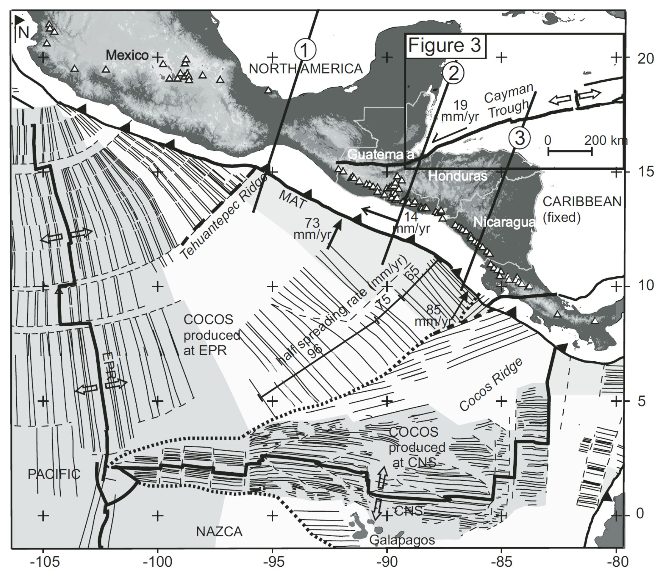
Present setting of Central America showing plates, Cocos crust produced at East Pacifi c Rise (EPR), and Cocos-Nazca spreading center (CNS), triple-junction trace (heavy dotted line), volcanoes (open triangles), Middle America Trench (MAT), and rates of relative plate motion (DeMets et al., 2000; DeMets, 2001). East Pacifi c Rise half spreading rates from Wilson (1996) and Barckhausen et al. (2001). Lines 1, 2, and 3 are locations of topographic and tomographic profi les in Figure 6.
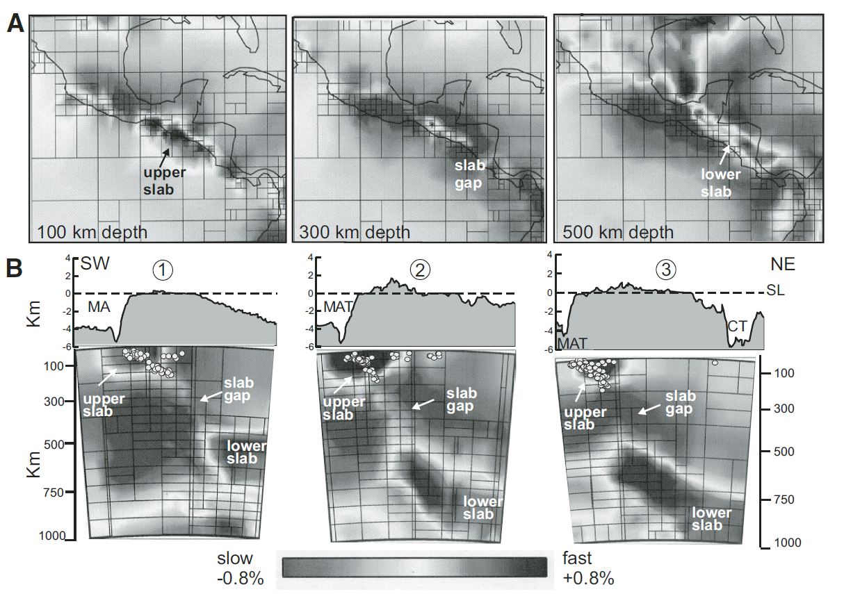
(A) Tomographic slices of the P-wave velocity of the mantle at depths of 100, 300, and 500 km beneath Central America. (B) Upper panels show cross sections of topography and bathymetry. Lower panels: tomographic profi les showing Cocos slab detached below northern Central America, upper Cocos slab continuous with subducted plate at Middle America Trench (MAT), and slab gap between 200 and 500 km. Shading indicates anomalies in seismic wave speed as a ±0.8% deviation from average mantle velocities. Darker shading indicates colder, subducted slab material of Cocos plate. Circles are earthquake hypocenters. Grid sizes on profi les correspond to quantity of ray-path data within that cell of model; smaller boxes indicate regions of increased data density. CT—Cayman trough; SL—sea level (modifi ed from Rogers et al., 2002).
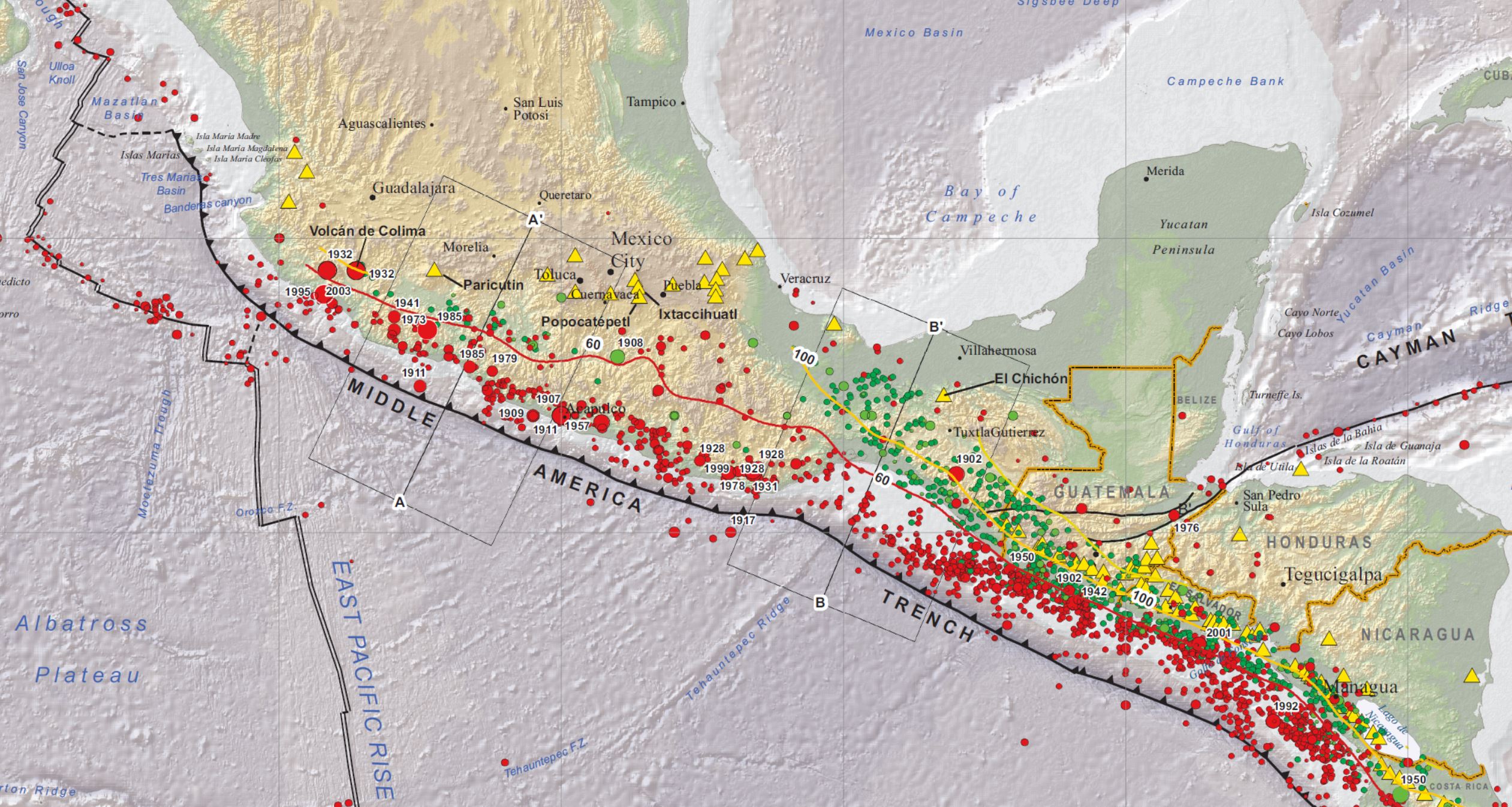
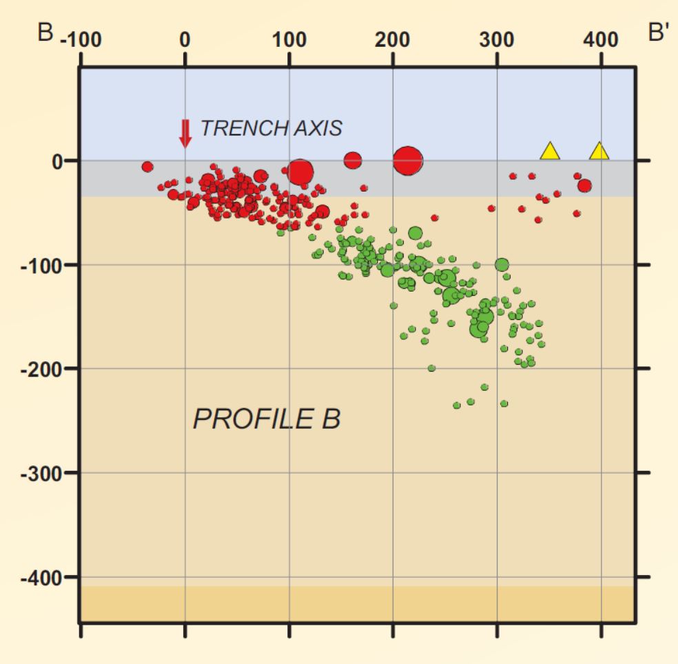
- These figures are from the USGS publication (Benz et al., 2011) that presents an educational poster about the historic seismicity and seismic hazard along the Middle America Trench.
- First is a map showing earthquake depth as color (green depth > red). Seismicity cross section B-B’ is shown on the map. Today’s M=6.6 quake is nearest this section.
- Franco et al. (2012) used GPS observations to evaluate the kinematics (how the plates move and interact relative to each other) of this region. Below is a map that shows earthquake mechanisms that reveal the strike-slip faults as they converge. The forearc sliver (the block between the megathrust and the forearc sliver fault) is shaded gray.
- These authors also use a model to estimate how much the megathrust is locked and accumulating elastic strain. They evaluate a range of possible physical properties of the find that the megathrust north of the forearc sliver is more highly locked (seismogenically coupled).
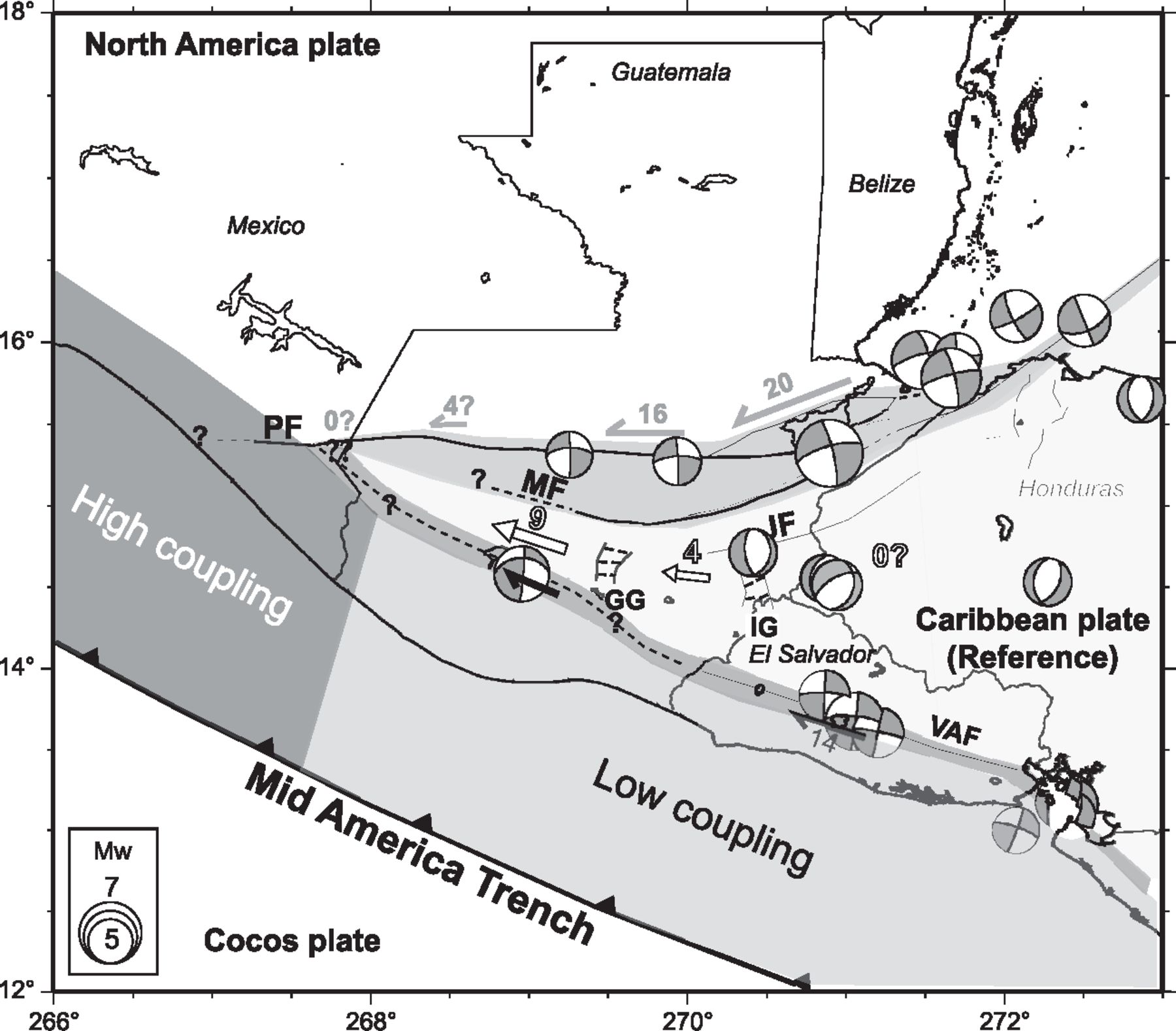
Proposed model of faults kinematics and coupling along the Cocos slab interface, revised from Lyon-Caen et al. (2006). Numbers are velocities relative to CA plate in mmyr−1. Focal mechanisms are for crustal earthquakes (depth ≤30 km) since 1976, from CMT Harvard catalogue.
- Here is a map from Benz et al. (2011) that shows the seismic hazard for this region.

- Below is a video that explains seismic tomography from IRIS.
Geologic Fundamentals
- For more on the graphical representation of moment tensors and focal mechnisms, check this IRIS video out:
- Here is a fantastic infographic from Frisch et al. (2011). This figure shows some examples of earthquakes in different plate tectonic settings, and what their fault plane solutions are. There is a cross section showing these focal mechanisms for a thrust or reverse earthquake. The upper right corner includes my favorite figure of all time. This shows the first motion (up or down) for each of the four quadrants. This figure also shows how the amplitude of the seismic waves are greatest (generally) in the middle of the quadrant and decrease to zero at the nodal planes (the boundary of each quadrant).

- Here is another way to look at these beach balls.
The two beach balls show the stike-slip fault motions for the M6.4 (left) and M6.0 (right) earthquakes. Helena Buurman's primer on reading those symbols is here. pic.twitter.com/aWrrb8I9tj
— AK Earthquake Center (@AKearthquake) August 15, 2018
- There are three types of earthquakes, strike-slip, compressional (reverse or thrust, depending upon the dip of the fault), and extensional (normal). Here is are some animations of these three types of earthquake faults. The following three animations are from IRIS.
Strike Slip:
Compressional:
Extensional:
- This is an image from the USGS that shows how, when an oceanic plate moves over a hotspot, the volcanoes formed over the hotspot form a series of volcanoes that increase in age in the direction of plate motion. The presumption is that the hotspot is stable and stays in one location. Torsvik et al. (2017) use various methods to evaluate why this is a false presumption for the Hawaii Hotspot.
- Here is a map from Torsvik et al. (2017) that shows the age of volcanic rocks at different locations along the Hawaii-Emperor Seamount Chain.

A cutaway view along the Hawaiian island chain showing the inferred mantle plume that has fed the Hawaiian hot spot on the overriding Pacific Plate. The geologic ages of the oldest volcano on each island (Ma = millions of years ago) are progressively older to the northwest, consistent with the hot spot model for the origin of the Hawaiian Ridge-Emperor Seamount Chain. (Modified from image of Joel E. Robinson, USGS, in “This Dynamic Planet” map of Simkin and others, 2006.)

Hawaiian-Emperor Chain. White dots are the locations of radiometrically dated seamounts, atolls and islands, based on compilations of Doubrovine et al. and O’Connor et al. Features encircled with larger white circles are discussed in the text and Fig. 2. Marine gravity anomaly map is from Sandwell and Smith.
- 2019.02.01 M 6.6 Guatemala & Mexico
- 2018.02.16 M 7.2 Oaxaca, Mexico
- 2018.01.19 M 6.3 Gulf of California
- 2017.09.19 M 7.1 Puebla, Mexico
- 2017.09.19 M 7.1 Puebla, Mexico Update #1
- 2017.09.08 M 8.1 Chiapas, Mexico
- 2017.09.08 M 8.1 Chiapas, Mexico Update #1
- 2017.09.23 M 8.1 Chiapas, Mexico Update #2
- 2017.06.22 M 6.8 Guatemala
- 2017.06.14 M 6.9 Guatemala
- 2017.05.12 M 6.2 El Salvador
- 2017.03.29 M 5.7 Gulf of California
- 2016.11.24 M 7.0 El Salvador
- 2016.04.29 M 6.6 East Pacific Rise / MAT
- 2016.01.21 M 6.6 Mexico
- 2015.09.13 M 6.6 Gulf California
- 2015.09.13 M 6.6 Gulf California Update #1
- 2014.10.14 M 7.3 El Salvador
- 2013.10.20 M 6.4 Gulf California
Mexico | Central America
Earthquake Reports
Social Media
“When a fault slips during an #earthquake, there are changes in stress in the surrounding crust. These changes can either promote or inhibit the subsequent earthquake, depending on the orientation and type of fault on which the stress is imparted.” https://t.co/Qj4iOTQLwR
— Dr Lucy Jones Center (@DLJCSS) February 3, 2019
- Benz, H.M., Dart, R.L., Villaseñor, Antonio, Hayes, G.P., Tarr, A.C., Furlong, K.P., and Rhea, Susan, 2011 a. Seismicity of the Earth 1900–2010 Mexico and vicinity: U.S. Geological Survey Open-File Report 2010–1083-F, scale 1:8,000,000.
- Franco, A., Lasserre, C., Lyon-Caen, H., Kostoglodov, V., Molina, E., Guzman-Speziale, M., Monterosso, D., Robles, V., Figueroa, C., Amaya, W., Barrier, E., Chiquin, L., Moran, S., Flores, O., Romero, J., Santiago, J.A., Manea, M., Manea, V.C., 2012. Fault kinematics in northern Central America and coupling along the subduction interface of the Cocos Plate, from GPS data in Chiapas (Mexico), Guatemala and El Salvador in Geophysical Journal International., v. 189, no. 3, p. 1223-1236 https://doi.org/10.1111/j.1365-246X.2012.05390.x
- Frisch, W., Meschede, M., Blakey, R., 2011. Plate Tectonics, Springer-Verlag, London, 213 pp.
- Hayes, G., 2018, Slab2 – A Comprehensive Subduction Zone Geometry Model: U.S. Geological Survey data release, https://doi.org/10.5066/F7PV6JNV.
- Manea, V.C., Manea, M., and Ferrari, L., 2013. A geodynamical perspective on the subduction of Cocos and Rivera plates beneath Mexico and Central America in Tectonophysics, http://doi.org/10.1016/j.tecto.2012.12.039
- Mann, P., 2007, Overview of the tectonic history of northern Central America, in Mann, P., ed., Geologic and tectonic development of the Caribbean plate boundary
in northern Central America: Geological Society of America Special Paper 428, p. 1–19, https://doi.org/10.1130/2007.2428(01). - Meyer, B., Saltus, R., Chulliat, a., 2017. EMAG2: Earth Magnetic Anomaly Grid (2-arc-minute resolution) Version 3. National Centers for Environmental Information, NOAA. Model. http://doi:10.7289/V5H70CVX
- Meyer, B., Saltus, R., Chulliat, a., 2017. EMAG2: Earth Magnetic Anomaly Grid (2-arc-minute resolution) Version 3. National Centers for Environmental Information, NOAA. Model. http://doi:10.7289/V5H70CVX
- Müller, R.D., Sdrolias, M., Gaina, C. and Roest, W.R., 2008, Age spreading rates and spreading asymmetry of the world’s ocean crust in Geochemistry, Geophysics, Geosystems, 9, Q04006, http://doi:10.1029/2007GC001743
References:
Return to the Earthquake Reports page.