
There was just now an earthquake in Oaxaca, Mexico between the other large earthquakes from last 2017.09.08 (M 8.1) and 2017.09.08 (M 7.1). There has already been a M 5.8 aftershock.Here is the USGS website for today’s M 7.2 earthquake.
This M 7.2 earthquake has a depth that is close to where we think the subduction zone fault is. Currently, the hypocentral depth is 24.7 km and the depth to the slab based upon the Hayes et al. (2012) Slab 1.0 model is about 40 km. So this earthquake may be in the upper North America plate and not on the subduction zone.
UPDATE: The SSN has a reported depth of 12 km, further supporting evidence that this earthquake was in the North America plate.
This region of the subduction zone dips at a very shallow angle (flat and almost horizontal).
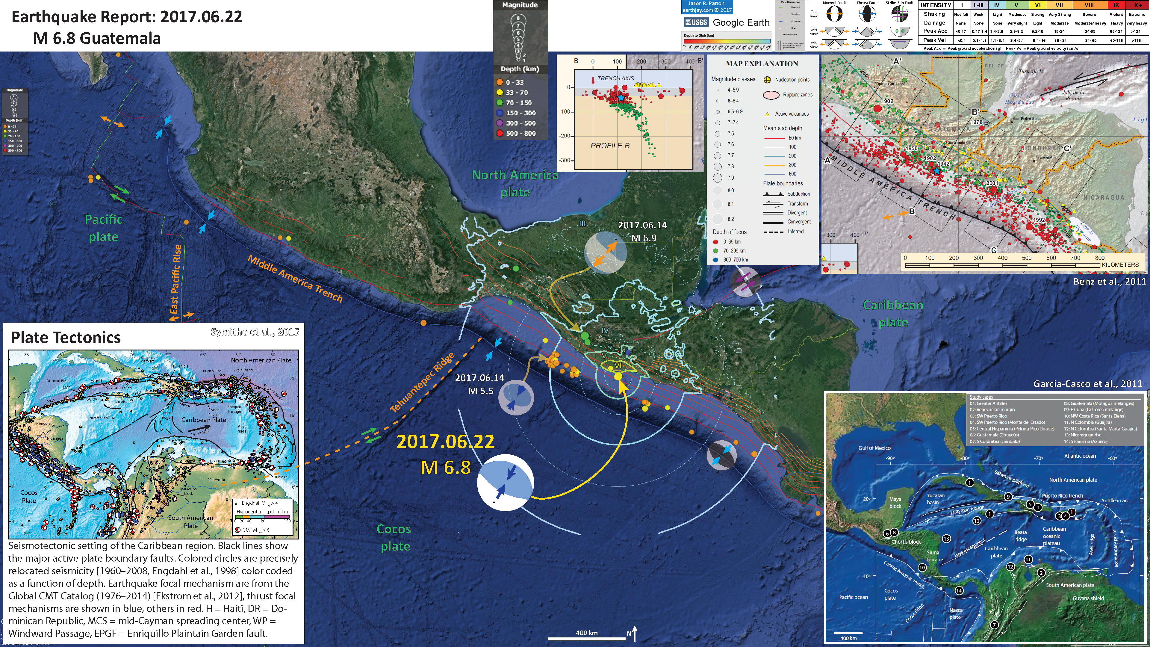
There was also a sequence of earthquakes offshore of Guatemala in June, which could possibly be related to the M 8.1 earthquake. Here is my earthquake report for the Guatemala earthquake.
The poster also shows the seismicity associated with the M 7.6 earthquake along the Swan fault (southern boundary of the Cayman trough). Here is my earthquake report for the Guatemala earthquake.
Today’s earthquake happened in a region that had a slightly elevated static coulomb stress following the 2017.09.08 M 8.1 earthquake as calculated by Shinji Toda from Temblor.
UPDATE: I misinterpreted the stress change results as noticed by Eric Fielding:
Coulomb stress change map from Temblor was for receiver faults with orientation of the September M7.1 normal quake, not thrust faults like February M7.2, so effects will be different
— Eric Fielding (@EricFielding) February 17, 2018
- Here are my earthquake reports for these two recent earthquakes in Mexico
- 2017.09.19 M 7.1 Puebla, Mexico
- 2017.09.19 M 7.1 Puebla, Mexico Update #1
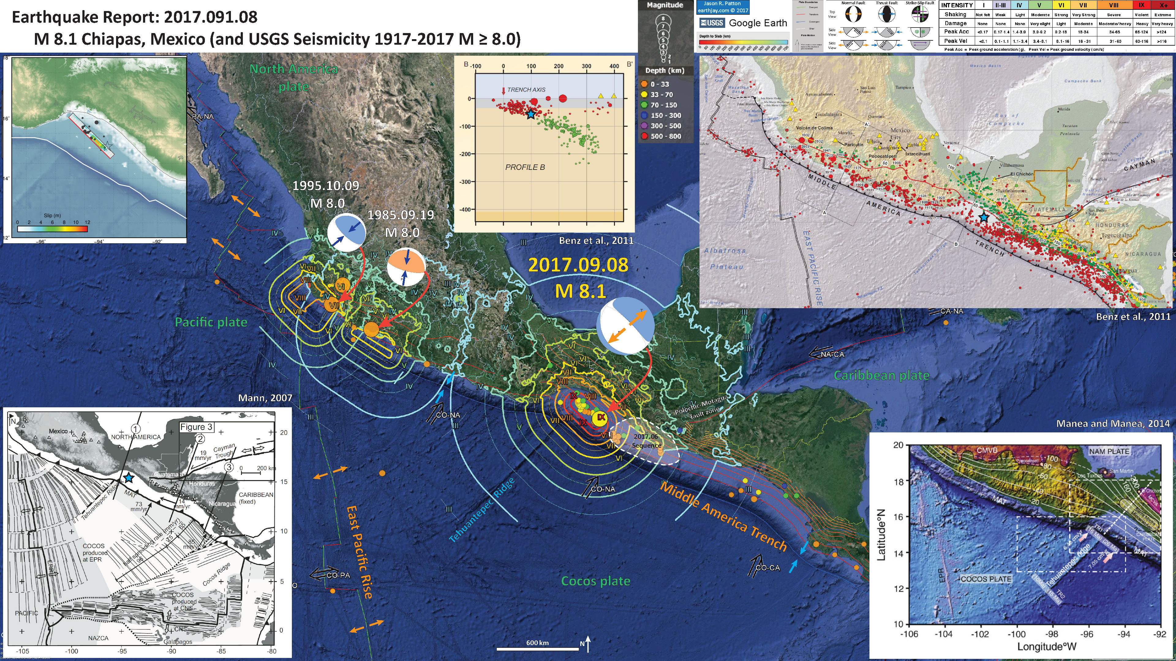
- 2017.09.08 M 8.1 Chiapas, Mexico
- 2017.09.08 M 8.1 Chiapas, Mexico Update #1
- 2017.09.23 M 8.1 Chiapas, Mexico Update #2
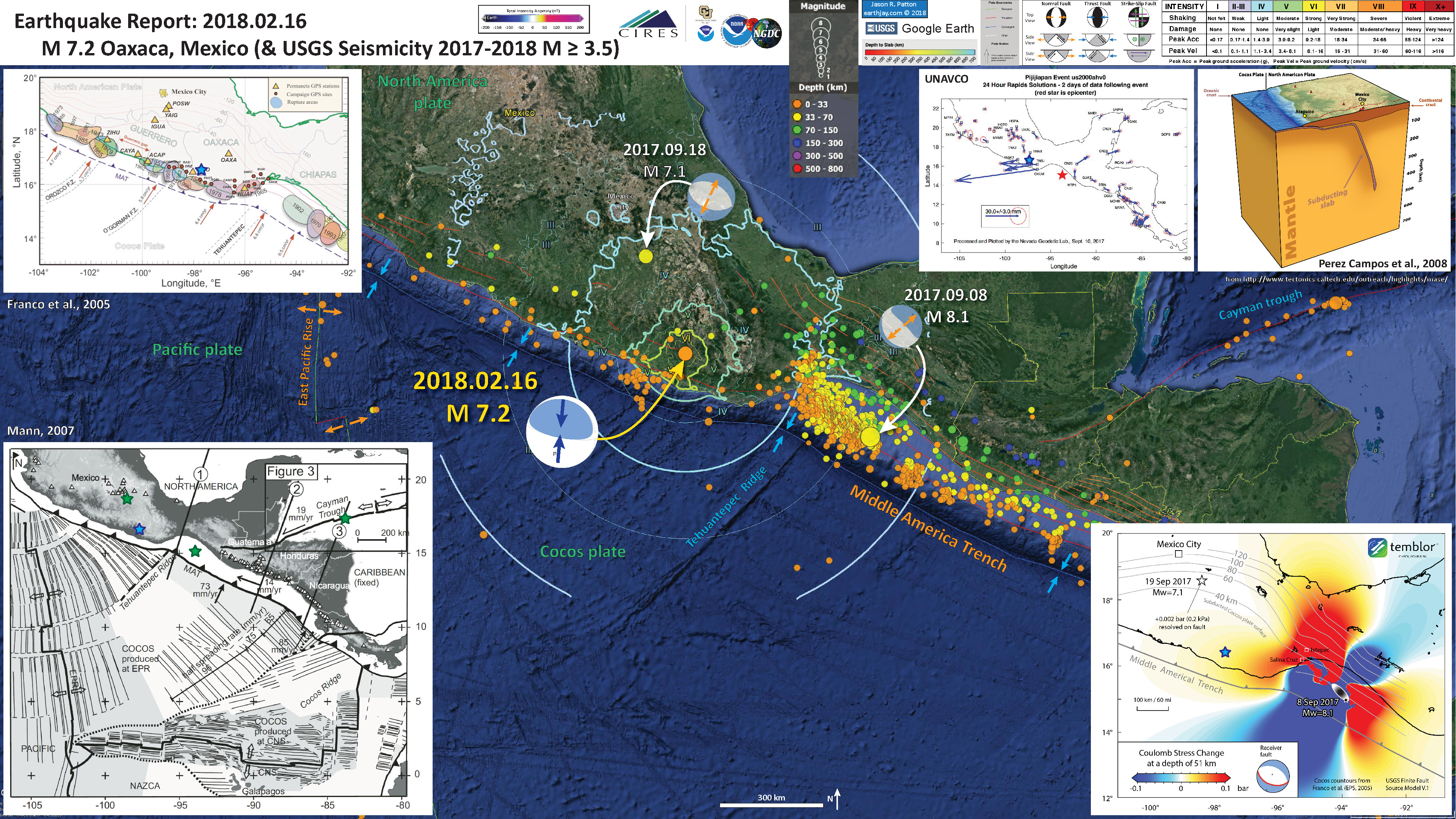
Below is my interpretive poster for this earthquake
I plot the seismicity from the past year, with color representing depth and diameter representing magnitude (see legend). I include earthquake epicenters from 1918-2018 with magnitudes M ≥ 3.5.
Note the difference in aftershock patterns between the shallower M 8.2 earthquake and the deeper M 7.1 earthquake. (hint: the deep M 8.1 did not have any aftershocks)
I plot the USGS fault plane solutions (moment tensors in blue and focal mechanisms in orange) for the M 7.2 earthquake, in addition to some relevant recent earthquakes.
- I placed a moment tensor / focal mechanism legend on the poster. There is more material from the USGS web sites about moment tensors and focal mechanisms (the beach ball symbols). Both moment tensors and focal mechanisms are solutions to seismologic data that reveal two possible interpretations for fault orientation and sense of motion. One must use other information, like the regional tectonics, to interpret which of the two possibilities is more likely.
- I also include the shaking intensity contours on the map. These use the Modified Mercalli Intensity Scale (MMI; see the legend on the map). This is based upon a computer model estimate of ground motions, different from the “Did You Feel It?” estimate of ground motions that is actually based on real observations. The MMI is a qualitative measure of shaking intensity. More on the MMI scale can be found here and here. This is based upon a computer model estimate of ground motions, different from the “Did You Feel It?” estimate of ground motions that is actually based on real observations.
- We can observe that Mexico City even shook more strongly due to the basin effects. Mexico City is locate on the map and there is a MMI IV.5 contour that surrounds the large valley. Mexico City was hit strongly by a M 8.0 earthquake in 1985 and again last September. See my report for more about the basin amplification.
- I include the slab contours plotted (Hayes et al., 2012), which are contours that represent the depth to the subduction zone fault. These are mostly based upon seismicity. The depths of the earthquakes have considerable error and do not all occur along the subduction zone faults, so these slab contours are simply the best estimate for the location of the fault.
-
I include some inset figures.
- In the lower left corner is a map from Mann (2007) that shows the regional tectonics. Plate boundary faults are in bold line, while lineations representing the spreading history are represented by thinner lines. I place a blue star in the general location of tonight’s M 7.2 earthquake (also in other inset maps) and green stars for the other 3 earthquakes discussed here.
- In the upper right corner is a figure from Perez and Campos (2008; as presented here) which shows the interpreted geometry of the subducting slab in this region. The profile of the seismic array used as a basis for this interpretation (the MASE array) is denoted by the brown dashed line. This line is also shown on the figure in the lower right corner).
- To the left of the cross section is a plot showing a 2 day solution for GPS positions in this region following the M 8.1 earthquake. Note how today’s M 7.2 earthquake (the blue star) is in an area that moved significantly during and following the M 8.1 earthquake.
- In the lower right corner is a figure prepared by Temblor here, a company that helps people learn and prepare to be more resilient given a variety of natural hazards. This figure is the result of numerical modeling of static coulomb stress changes in the lithosphere following the 2017 M 8.1 earthquake. This basically means that regions that are red have an increased stress (an increased likelihood for an earthquake) following the earthquake, while blue represents a lower stress, or likelihood. The change in stress are very very small compared to the overall stress on any tectonic fault. This means that an earthquake may be triggered from this change in stress ONLY IF the fault is already highly strained (i.e. that the fault is about ready to generate an earthquake within a short time period, like a day, month, or year or so). The take away: the M 8.1 earthquake did not increase the stress on faults in the region of the M 7.1 (Temblor suggests the amount of increased stress near the M 7.1 is about the amount of force it takes to snap one’s fingers).
However, today’s M 7.2 earthquake did have an increase in the stress on faults in the region of the M 7.1 earthquake. - In the upper left corner is a map that shows some historic earthquake patches along the Middle America Trench. Today’s earthquake happened near the and 1978 M 7.7 earthquake and a 1999 M 7.5 earthquake not shown on this map (but in region of the 1968 earthquake.
Relevant Interpretive Posters
- 2017.06.22 M 6.8 Guatemala
- 2017.06.14 M 6.9 Guatemala
- 2017.09.08 M 8.1 Chiapas, Mexico
- 2017.09.08 M 8.1 Chiapas, Mexico Update #1
- 2017.09.23 M 8.1 Chiapas, Mexico Update #2
- 2017.09.19 M 7.1 Puebla, Mexico
- 2017.09.19 M 7.1 Puebla, Mexico Update #1

Some Relevant Discussion and Figures
- Here is the Franco et al. (2012) tectonic map.
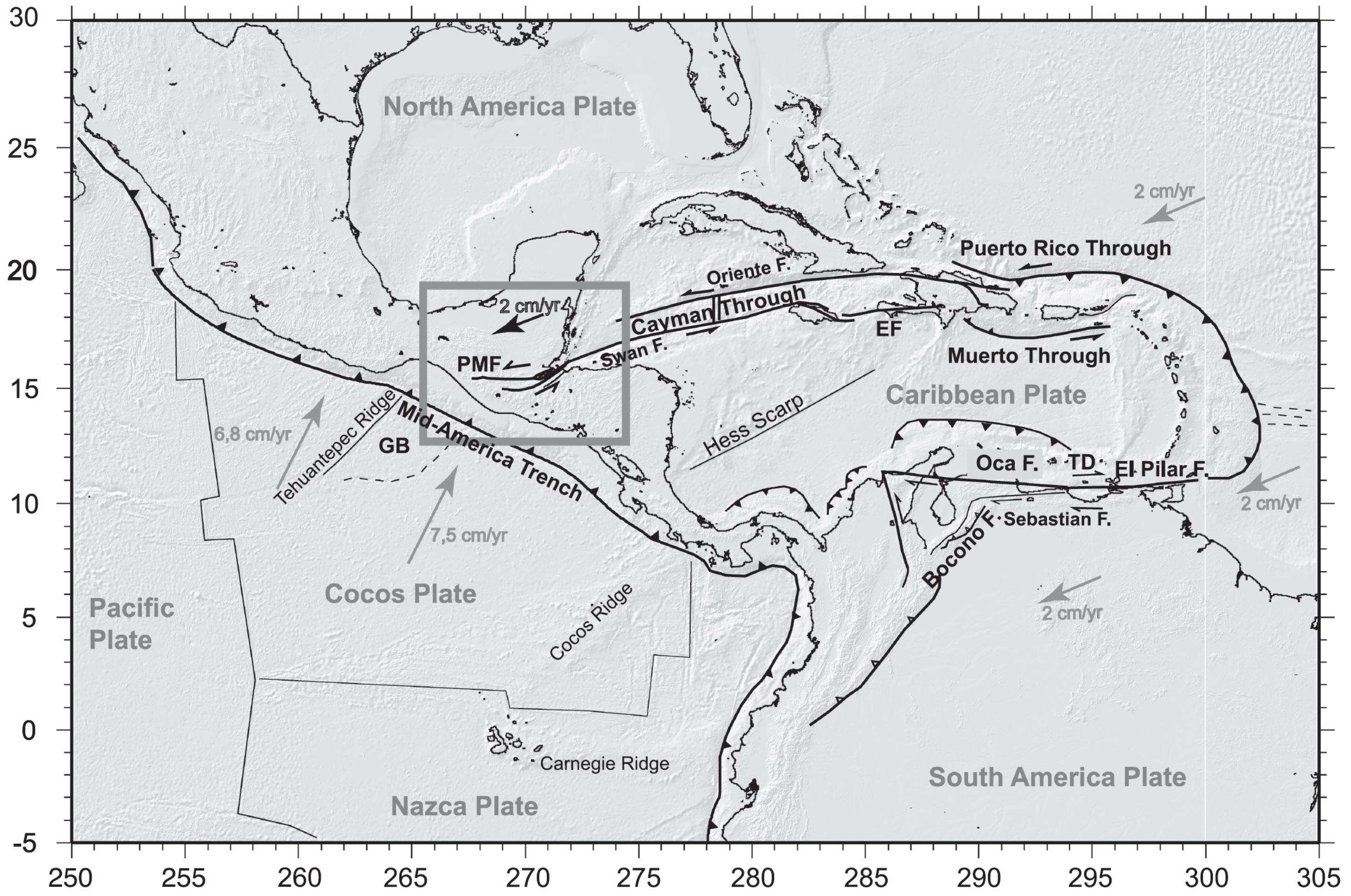
Tectonic setting of the Caribbean Plate. Grey rectangle shows study area of Fig. 2. Faults are mostly from Feuillet et al. (2002). PMF, Polochic–Motagua faults; EF, Enriquillo Fault; TD, Trinidad Fault; GB, Guatemala Basin. Topography and bathymetry are from Shuttle Radar Topography Mission (Farr&Kobrick 2000) and Smith & Sandwell (1997), respectively. Plate velocities relative to Caribbean Plate are from Nuvel1 (DeMets et al. 1990) for Cocos Plate, DeMets et al. (2000) for North America Plate and Weber et al. (2001) for South America Plate.
- Here is the figure from Gérault et al. (2015) that shows the slab contours.

(a) Geodynamic context of southwestern Mexico. Topography and bathymetry from ETOPO1 [Amante and Eakins, 2009]. A white curve outlines the Trans-Mexican Volcanic Belt (TMVB) [Ferrari et al., 2012]. The black lines show the isodepths of the Cocos slab at a 20 km interval, using seismicity up to ∼45 km depth and tomography below [Kim et al., 2012a]. These slab contours show that distinct topographic domains are associated with variations in slab geometry. The yellow vector shows the relative convergence velocity between the Cocos and North America Plate near Acapulco, holding North America fixed [DeMets et al., 2010]. The pink circles show the locations of the Meso-America Subduction Experiment (MASE) stations. (b) Moho depth (red) and upper slab limit (blue) from Kim et al. [2012a, 2013]. The dashed line shows the simplified Moho depth that we used in the numerical models. (c) Measured and smoothed topography along the MASE profile as a function of the distance from the southernmost seismic station, near Acapulco. The topography is smoothed using three passages of a rectangular sliding average of width 15 km.
- Here are some figures from Pérez-Campos et al. (2008) that show results from the MASE seismic experiment. First is the map showing the seismic array in the tectonic context.
- These authors used receiver functions to estimate the depth to the Cocos plate (the slab depth). Below is their figure showing their results. Receiver function analyses use an array (a linear network, or grid network, but a linear network in this case) of seismometers. “A receiver function technique is a way to model the structure of the Earth by using the information from teleseismic earthquakes recorded at a three component seismograph.” More can be found on this here and here.
- And finally, here is their model of the subducting slab. The authors also use seismic tomography to evaluate the geometry of the plates in this region. Seismic tomography is the same as a CT scan of the Earth. We can think of seismic tomography as a 3-D X-Ray of the Earth, just using seismic waves instead.

MASE seismic array. Slab isodepth contours from Pardo and Sua´rez [1995] are in blue dashed lines. The dots represent epicenters of M>4 earthquakes, reported by the Servicio Sismolo´gico Nacional (SSN; in pink) from December 2004 through June 2007 and those re-located by Pardo and Sua´rez [1995] (in green). The thick orange line represents the profile of Figures 2 and 3. The arrows indicate the beginning (dark blue) and end (light blue) of the flat segment, and the tip of the slab (red).

Receiver function images. The black triangles denote the position of the stations along the profile with elevation exaggerated 10 times. The thick brown line denotes the extent of the TMVB. Seismicity (SSN: pink; Pardo and Sua´rez [1995]: green), within 50 km of the MASE profile, is shown as dots. The bottom left plot shows RFs for one teleseismic event along the flat slab portion of the slab; the bottom middle plot illustrates the corresponding model (LVM = low velocity mantle and OC = oceanic crust). Compressional-wave velocity models A, B, and C shown in the bottom right plot were determined from waveform modeling of RFs. They correspond to the structure at A, B, and C of the bottom left plot.

Composite model: tomographic and RF image showing the flat and descending segments of the slab. The key features are the flat under-plated subduction for 250 km, and the location and truncation of the slab at 500 km. The zone separating the ocean crust from the continental Moho is estimated to be less than 10 km in thickness. NA = North America, C = Cocos, LC = lower crust, LVM = low velocity mantle, OC = oceanic crust.
Some Background Materials
- For more on the graphical representation of moment tensors and focal mechnisms, check this IRIS video out:
- Here is a fantastic infographic from Frisch et al. (2011). This figure shows some examples of earthquakes in different plate tectonic settings, and what their fault plane solutions are. There is a cross section showing these focal mechanisms for a thrust or reverse earthquake. The upper right corner includes my favorite figure of all time. This shows the first motion (up or down) for each of the four quadrants. This figure also shows how the amplitude of the seismic waves are greatest (generally) in the middle of the quadrant and decrease to zero at the nodal planes (the boundary of each quadrant).

- There are three types of earthquakes, strike-slip, compressional (reverse or thrust, depending upon the dip of the fault), and extensional (normal). Here is are some animations of these three types of earthquake faults. Many of the earthquakes people are familiar with in the Mendocino triple junction region are either compressional or strike slip. The following three animations are from IRIS.
- Below is a video that explains seismic tomography from IRIS.
- Here is an educational animation from IRIS that helps us learn about how different earth materials can lead to different amounts of amplification of seismic waves. Recall that Mexico City is underlain by lake sediments with varying amounts of water (groundwater) in the sediments.
- Here is an educational video from IRIS that helps us learn about resonant frequency and how buildings can be susceptible to ground motions with particular periodicity, relative to the building size.
- 2018.02.16 M 7.2 Oaxaca, Mexico
- 2018.01.19 M 6.3 Gulf of California
- 2017.09.19 M 7.1 Puebla, Mexico
- 2017.09.19 M 7.1 Puebla, Mexico Update #1
- 2017.09.08 M 8.1 Chiapas, Mexico
- 2017.09.08 M 8.1 Chiapas, Mexico Update #1
- 2017.09.23 M 8.1 Chiapas, Mexico Update #2
- 2017.06.22 M 6.8 Guatemala
- 2017.06.14 M 6.9 Guatemala
- 2017.05.12 M 6.2 El Salvador
- 2017.03.29 M 5.7 Gulf of California
- 2016.11.24 M 7.0 El Salvador
- 2016.04.29 M 6.6 East Pacific Rise / MAT
- 2016.01.21 M 6.6 Mexico
- 2015.09.13 M 6.6 Gulf California
- 2015.09.13 M 6.6 Gulf California Update #1
- 2014.10.14 M 7.3 El Salvador
- 2013.10.20 M 6.4 Gulf California
- Benz, H.M., Dart, R.L., Villaseñor, Antonio, Hayes, G.P., Tarr, A.C., Furlong, K.P., and Rhea, Susan, 2011 a. Seismicity of the Earth 1900–2010 Mexico and vicinity: U.S. Geological Survey Open-File Report 2010–1083-F, scale 1:8,000,000.
- Benz, H.M., Tarr, A.C., Hayes, G.P., Villaseñor, Antonio, Furlong, K.P., Dart, R.L., and Rhea, Susan, 2011 b. Seismicity of the Earth 1900–2010 Caribbean plate and vicinity: U.S. Geological Survey Open-File Report 2010–1083-A, scale 1:8,000,000.
- Cruz-Atienza et al., 2016. Long Duration of Ground Motion in the Paradigmatic Valley of Mexico in Scientific Reports, v. 6, DOI: 10.1038/srep38807
- Franco, A., C. Lasserre H. Lyon-Caen V. Kostoglodov E. Molina M. Guzman-Speziale D. Monterosso V. Robles C. Figueroa W. Amaya E. Barrier L. Chiquin S. Moran O. Flores J. Romero J. A. Santiago M. Manea V. C. Manea, 2012. Fault kinematics in northern Central America and coupling along the subduction interface of the Cocos Plate, from GPS data in Chiapas (Mexico), Guatemala and El Salvador in Geophysical Journal International., v. 189, no. 3, p. 1223-1236. DOI: https://doi.org/10.1111/j.1365-246X.2012.05390.x
- Franco, S.I., Kostoglodov, V., Larson, K.M., Manea, V.C>, Manea, M., and Santiago, J.A., 2005. Propagation of the 2001–2002 silent earthquake and interplate coupling in the Oaxaca subduction zone, Mexico in Earth Planets Space, v. 57., p. 973-985.
- Frisch, W., Meschede, M., Blakey, R., 2011. Plate Tectonics, Springer-Verlag, London, 213 pp.
- Garcia-Casco, A., Projenza, J.A., Iturralde-Vinent, M.A., 2011. Subduction Zones of the Caribbean: the sedimentary, magmatic, metamorphic and ore-deposit records UNESCO/iugs igcp Project 546 Subduction Zones of the Caribbean in Geologica Acta, v. 9, no., 3-4, p. 217-224
- Gérault, M., Husson, L., Miller, M.S., and Humphreys, E.D., 2015. Flat-slab subduction, topography, and mantle dynamics in southwestern Mexico in Tectonics, v. 34, p. 1892-1909, doi:10.1002/2015TC003908.
- Quzman-Speziale, M. and Zunia, F.R., 2015. Differences and similarities in the Cocos-North America and Cocos-Caribbean convergence, as revealed by seismic moment tensors in Journal of South American Earth Sciences, http://dx.doi.org/10.1016/j.jsames.2015.10.002
- Hayes, G. P., D. J. Wald, and R. L. Johnson, 2012. Slab1.0: A three-dimensional model of global subduction zone geometries, J. Geophys. Res., 117, B01302, doi:10.1029/2011JB008524.
- Lay et al., 2011. Outer trench-slope faulting and the 2011 Mw 9.0 off the Pacific coast of Tohoku Earthquake in Earth Planets Space, v. 63, p. 713-718.
- Manea, M., and Manea, V.C., 2014. On the origin of El Chichón volcano and subduction of Tehuantepec Ridge: A geodynamical perspective in JGVR, v. 175, p. 459-471.
- Mann, P., 2007, Overview of the tectonic history of northern Central America, in Mann, P., ed., Geologic and tectonic development of the Caribbean plate boundary in northern Central America: Geological Society of America Special Paper 428, p. 1–19, doi: 10.1130/2007.2428(01). For
- McCann, W.R., Nishenko S.P., Sykes, L.R., and Krause, J., 1979. Seismic Gaps and Plate Tectonics” Seismic Potential for Major Boundaries in Pageoph, v. 117
- Pérez-Campos, Z., Kim, Y., Husker, A., Davis, P.M. ,Clayton, R.W., Iglesias,k A., Pacheco, J.F., Singh, S.K., Manea, V.C., and Gurnis, M., 2008. Horizontal subduction and truncation of the Cocos Plate beneath central Mexico in GRL, v. 35, doi:10.1029/2008GL035127
- Polltz, F.F., Stein, R.S., Sevigen, V., Burgmann, R., 2012. The 11 April 2012 east Indian Ocean earthquake triggered large aftershocks worldwide in Nature, v. 000, doi:10.1038/nature11504
- Symithe, S., E. Calais, J. B. de Chabalier, R. Robertson, and M. Higgins, 2015. Current block motions and strain accumulation on active faults in the Caribbean in J. Geophys. Res. Solid Earth, v. 120, p. 3748–3774, doi:10.1002/2014JB011779.
Strike Slip:
Compressional:
Extensional:
Social Media
Interactive Earthquake Browser images showing 1) earthquakes in the region around the recent M7.2 in Mexico. 2) Earthquakes of M7.0+ in the same region. The current event is circled. https://t.co/KpNl88d90R #earthquake #Mexico pic.twitter.com/4OAZFo0307
— IRIS Earthquake Sci (@IRIS_EPO) February 17, 2018
Look at the seismic waves from the M7.2 #earthquake in #Mexico using this tool – https://t.co/BK7uFxUZEP. Simply choose a seismic station to see the data! (The image below is from a station in Panama) pic.twitter.com/PIAUJFBQA5
— IRIS Earthquake Sci (@IRIS_EPO) February 17, 2018
Mw=7.2, OAXACA, MEXICO (Depth: 20 km), 2018/02/16 23:39:42 UTC – Full details here: https://t.co/VGTOMqHuuX pic.twitter.com/MzQyca3JB1
— Earthquakes (@geoscope_ipgp) February 17, 2018
Seismic waves from the M7.2 Mexico earthquake rolled through #Victoria and #Vancouver a few minutes ago. Not felt in Canada – but easily recorded by our seismographs. The fastest-travelling P-waves took just under 7 minutes to travel nearly 4200 km. pic.twitter.com/fcZlFyf8U1
— John Cassidy (@earthquakeguy) February 17, 2018
Cross-section of seismicity near today's M7.2 indicates that the earthquake occurred in a region of flat slab subduction, near the bottom of the coupled zone, on the interface between the two plates. pic.twitter.com/9FERcjwo97
— Jascha Polet (@CPPGeophysics) February 17, 2018
Map of historical seismicity and recent (since September of 2017) large earthquakes in Mexico. Today's M7.2 is the first large subduction thrust earthquake in this sequence, on the interface between the two plates and not within the subducting slab. pic.twitter.com/hRKuyLpwJQ
— Jascha Polet (@CPPGeophysics) February 17, 2018
Although I have seen a few reports of this being a "seismic gap" rupturing subduction interface event, today's quake did not occur near a gap (map from https://t.co/FOf2ZYziMP red/white circle approximate location of today's M7.2) pic.twitter.com/sv0dmt4OgI
— Jascha Polet (@CPPGeophysics) February 17, 2018
Reportan los primeros daños por el #Sismo en Pinotepa Oaxaca. Aún sin víctimas que lamentar. Viviendas en la Costa, y tiendas en la colonia Reforma en la capital. pic.twitter.com/BdF1auXGif
— Alternativa Oaxaca (@AlternativaOAX) February 17, 2018
RAW VIDEO: Magnitude-7.2 earthquake slams Mexico. https://t.co/XaqZz8gq1w
— The Associated Press (@AP) February 17, 2018
La alerta sísmica de México se activó 72 Segundos antes de la llegada del sismo a CDMX
pic.twitter.com/aAALHiFzXQ— 🌏Tuitero Sismico 🌎 (@TuiteroSismico) February 17, 2018
Mexico City buildings sway in M=7.2 earthquake | https://t.co/1twVj9WIVY https://t.co/z2UhvZlBr6 via @temblor
— temblor (@temblor) February 17, 2018
Strong (M7.2) and shallow (12 km) #earthquake in Oaxaca state, Mexico, according to SSN https://t.co/YM26VKYT8E
— Stéphane Baize (@stef92320) February 17, 2018
My @raspishake caught the M7.2 Mexico earthquake from earlier today. pic.twitter.com/noOlPB5BGr
— Ryan Hollister (@phaneritic) February 17, 2018
Southern Mexico—Earthquakes, Tectonics, & Earthquake Early Warning https://t.co/bNzhZbsvrv #earthquakes #mexico pic.twitter.com/qNnGyzUlc5
— IRIS Earthquake Sci (@IRIS_EPO) February 17, 2018
Mexico earthquake: Strong tremor hits Oaxaca state – BBC News https://t.co/4gitQzX0Zh #Mexico #Oaxaca #earthquake
— Lauri Kinnunen (@energyenviro) February 17, 2018
Asi se sintió el #sismo de 7,2 en la redacción de @Milenio en #Mexico
El epicentro fue en Pinotepa Nacional, #Oaxacapic.twitter.com/xBcl2H4KG4
— Vini (@VinicioGarzon) February 17, 2018
Toda una tragedia. Al menos 13 muertos en el accidente del #helicóptero que supervisaba el #terremoto de #México https://t.co/wHfvSxmbZN pic.twitter.com/8jRNcf7HVC
— Sismo EQ (@sismoecuador) February 17, 2018
Video shows in 30 sec seismic activity in Pinotepa National , Mexico from Feb 15 to Feb 17@EricFielding @patton_cascadia @seismo_steve pic.twitter.com/IGQMR6IrAi
— ffloresm (@ffloresm) February 17, 2018
It is clear now that depth was probably close to correct but preliminary epicenters were probably about 30 km too far NE, as I also saw for M6.1 Ixtepec Earthquake in Oaxaca last September. https://t.co/UCLQjYpCKz
— Eric Fielding (@EricFielding) February 17, 2018