I am continuing to catch up on the Earthquake Reports for 2026. In June I was devoted to my fault trenching project. Then, later, I had total knee replacement surgery.
In June, there was a magnitude M 7.8 earthquake in the southern Philippines.
https://earthquake.usgs.gov/earthquakes/eventpage/us7000srb1/executive
The mainshock has a thrust earthquake mechanism (moment tensor). Thrust fault earthquakes are the result of horizontal compression.
The Philippine’s archipelago is quite complicated. Convergent plate boundary tectonics are the dominant driving force.
Due to the relative orientation of the plate boundaries, there are some large strike-slip faults that formed as strain and earthquake slip are partitioned along different faults. As for other natural systems, tectonic faults form to release stored energy in the most efficient way possible.
When plate convergence is misaligned to the plate boundaries (e.g., when the plates are converging in a direction perpendicular to the plate boundary, convergence is aligned and all tectonic strain and fault slip are localized along the subduction zone and associated thrust or reverse faults), the portion of the relative motion that is parallel to the boundary is consumed by strike-slip faults parallel to the plate boundary.
These are called forearc sliver faults. One good example of a forearc sliver fault is the Sumatra fault in Indonesia.
A forearc sliver fault has formed along central Philippines, called the Philippines fault.
The M 7.8 earthquake appears to be associated with the megathrust subduction zone that forms the Cotabato trench offshore of southwestern Mindanao, Philippines.
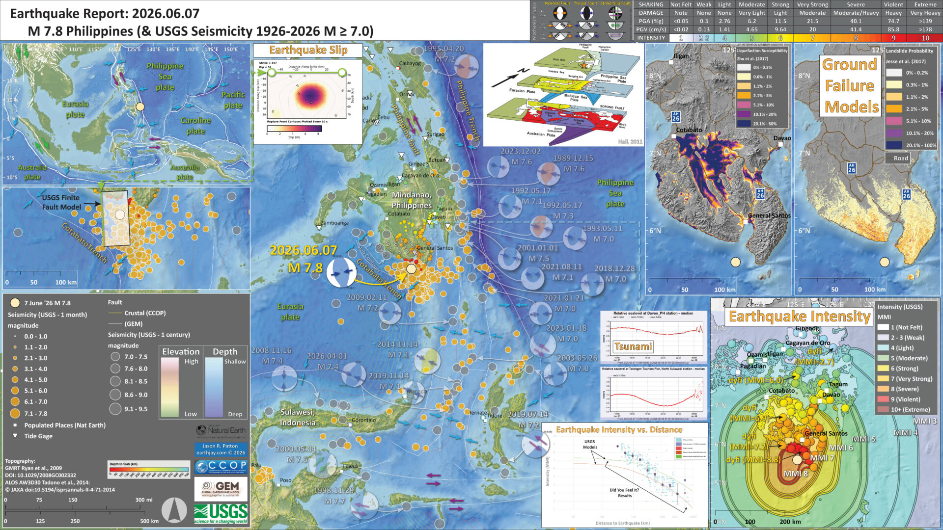
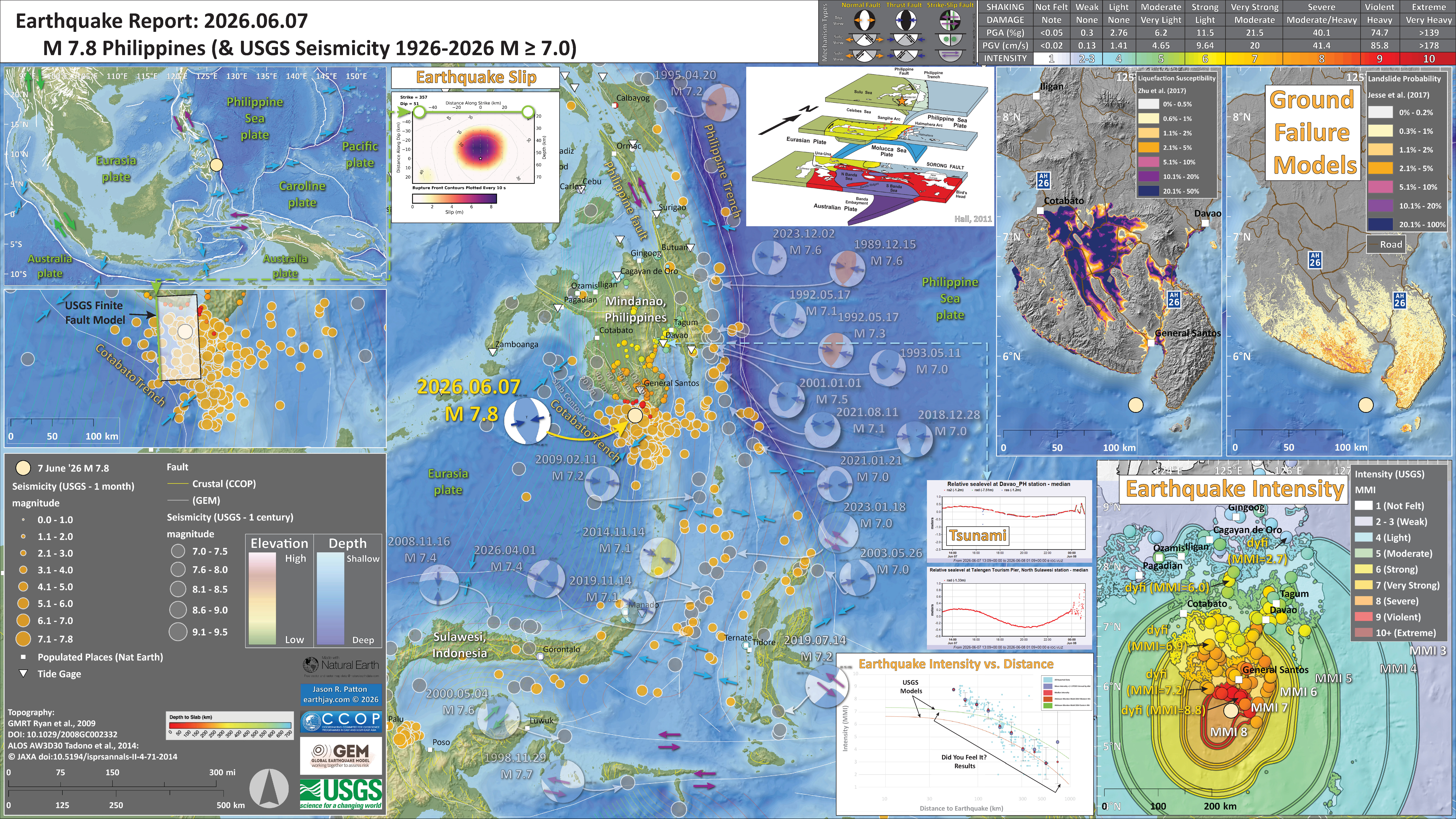
Below is my interpretive poster for this earthquake
- I plot the seismicity from the past month, with diameter representing magnitude (see legend). I include earthquake epicenters from 1926-2026 with magnitudes M ≥ 7.0 in one version.
- I plot the USGS fault plane solutions (moment tensors in blue and focal mechanisms in orange), possibly in addition to some relevant historic earthquakes.
- A review of the basic base map variations and data that I use for the interpretive posters can be found on the Earthquake Reports page. I have improved these posters over time and some of this background information applies to the older posters.
- Some basic fundamentals of earthquake geology and plate tectonics can be found on the Earthquake Plate Tectonic Fundamentals page.
- In the upper left corner is a small scale map showing the major plate boundaries.
- Below the tectonic overview map, on the left, is a large scale map showing the aftershock region for this M 7.8 earthquake sequence. I overlay the US Geological Survey finite fault slip model. The top of the fault that slipped is on the western edge of this ffm. The USGS estimates that the fault slipped up to about 8 meters.
- In the lower right corner is a map that shows the M 7.4 earthquake intensity using the modified Mercalli intensity scale. Earthquake intensity is a measure of how strongly the Earth shakes during an earthquake, so gets smaller the further away one is from the earthquake epicenter. The map colors represent a model of what the intensity may be. The USGS has a system called “Did You Feel It?” (DYFI) where people enter their observations from the earthquake and the USGS calculates what the intensity was for that person. The dots with yellow labels show what people actually felt in those different locations.
- To the left of the intensity map is a plot that shows the same intensity (both modeled and reported) data as displayed on the map. Note how the intensity gets smaller with distance from the earthquake.
- Above the intensity plot are two tide gage plots from Davao (location shown on map) and from Sulawesi (location not shown on map but the island is labeled).
- In the upper right corner is a map that shows the results of the USGS earthquake triggered landslide and earthquake induced liquefaction model. Read more about this model here.
- In the upper left is the USGS finite fault model that shows their estimate of the amount that the fault slipped during this earthquake.
- In the top-center is a map from Hall (2001) that shows the tectonic setting for the entire region. I place an orange star in the location of the M 7.8 earthquake.
I include some inset figures. Some of the same figures are located in different places on the larger scale map below.
- Here is the map with a month’s seismicity plotted.
Other Report Pages
Shaking Intensity
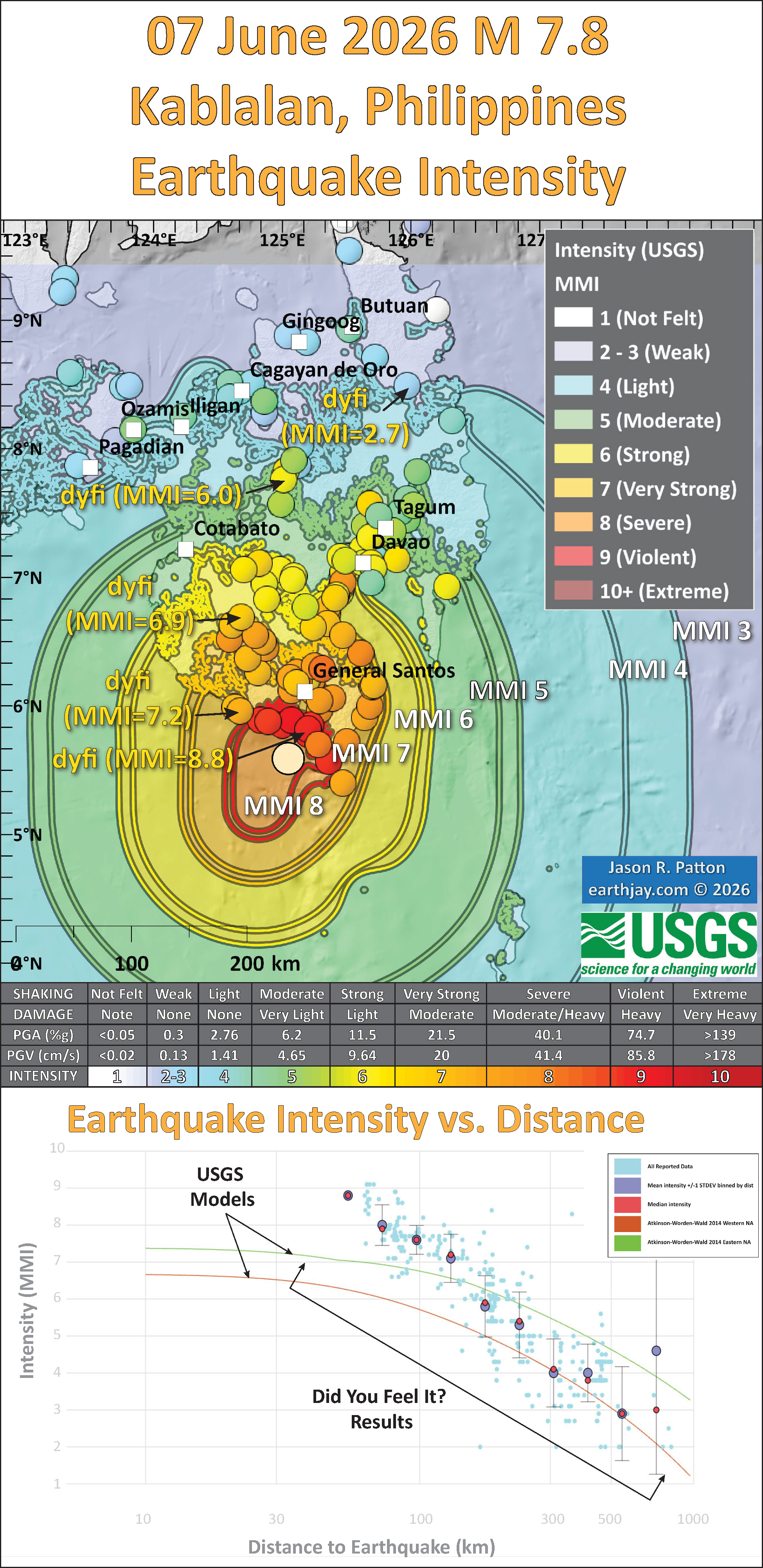
- Here is a figure that shows a more detailed comparison between the modeled intensity and the reported intensity. Both data use the same color scale, the Modified Mercalli Intensity Scale (MMI). More about this can be found here. The colors and contours on the map are results from the USGS modeled intensity. The DYFI data are plotted as colored dots (color = MMI, diameter = number of reports).
- In the upper panel is the USGS Did You Feel It reports map, showing reports as colored dots using the MMI color scale. Underlain on this map are colored areas showing the USGS modeled estimate for shaking intensity (MMI scale).
- In the lower panel is a plot showing MMI intensity (vertical axis) relative to distance from the earthquake (horizontal axis). The models are represented by the green and orange lines. The DYFI data are plotted as light blue dots. The mean and median (different types of “average”) are plotted as orange and purple dots. Note how well the reports fit the green line (the model that represents how MMI works based on quakes in California).
- Below the map and the lower plot is the USGS MMI Intensity scale, which lists the level of damage for each level of intensity, along with approximate measures of how strongly the ground shakes at these intensities, showing levels in acceleration (Peak Ground Acceleration, PGA) and velocity (Peak Ground Velocity, PGV).
Potential for Ground Failure
- Below are a series of maps that show the potential for landslides and liquefaction. These are all USGS data products.
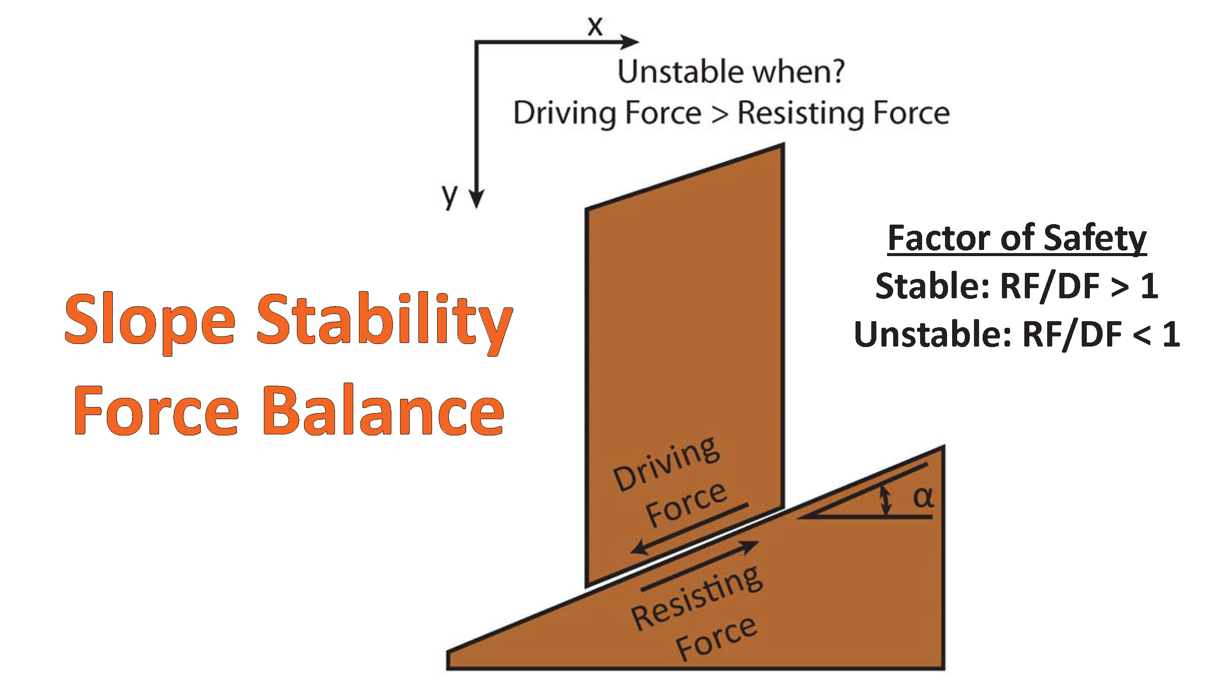
There are many different ways in which a landslide can be triggered. The first order relations behind slope failure (landslides) is that the “resisting” forces that are preventing slope failure (e.g. the strength of the bedrock or soil) are overcome by the “driving” forces that are pushing this land downwards (e.g. gravity). The ratio of resisting forces to driving forces is called the Factor of Safety (FOS). We can write this ratio like this:FOS = Resisting Force / Driving Force
- When FOS > 1, the slope is stable and when FOS < 1, the slope fails and we get a landslide. The illustration below shows these relations. Note how the slope angle α can take part in this ratio (the steeper the slope, the greater impact of the mass of the slope can contribute to driving forces). The real world is more complicated than the simplified illustration below.
- Landslide ground shaking can change the Factor of Safety in several ways that might increase the driving force or decrease the resisting force. Keefer (1984) studied a global data set of earthquake triggered landslides and found that larger earthquakes trigger larger and more numerous landslides across a larger area than do smaller earthquakes. Earthquakes can cause landslides because the seismic waves can cause the driving force to increase (the earthquake motions can “push” the land downwards), leading to a landslide. In addition, ground shaking can change the strength of these earth materials (a form of resisting force) with a process called liquefaction.
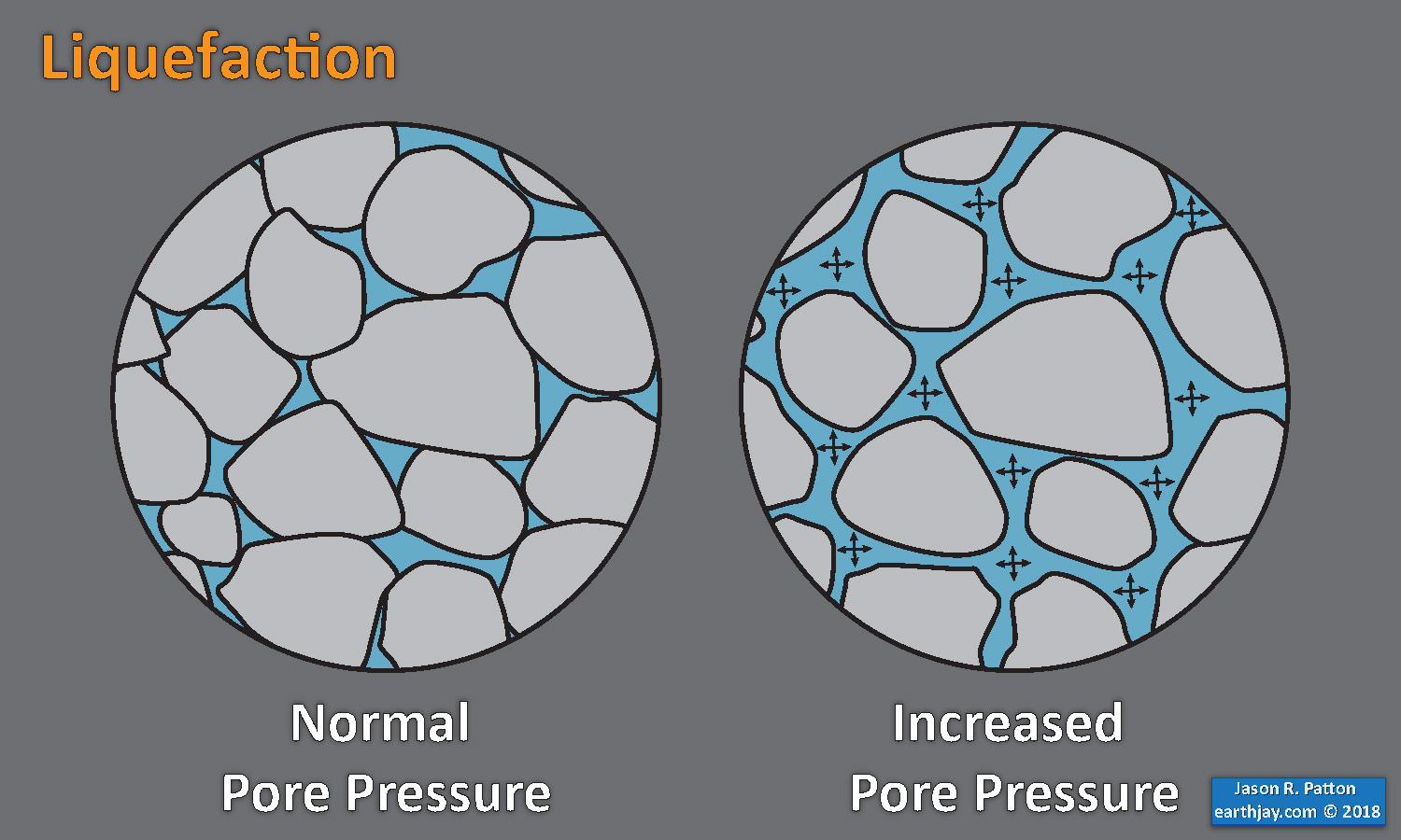
- Sediment or soil strength is based upon the ability for sediment particles to push against each other without moving. This is a combination of friction and the forces exerted between these particles. This is loosely what we call the “angle of internal friction.” Liquefaction is a process by which pore pressure increases cause water to push out against the sediment particles so that they are no longer touching.
- An analogy that some may be familiar with relates to a visit to the beach. When one is walking on the wet sand near the shoreline, the sand may hold the weight of our body generally pretty well. However, if we stop and vibrate our feet back and forth, this causes pore pressure to increase and we sink into the sand as the sand liquefies. Or, at least our feet sink into the sand.
- Below is a diagram showing how an increase in pore pressure can push against the sediment particles so that they are not touching any more. This allows the particles to move around and this is why our feet sink in the sand in the analogy above. This is also what changes the strength of earth materials such that a landslide can be triggered.
- Here Dr. Bohon demonstrates the phenomena of liquefaction.
- And, another video demonstration.
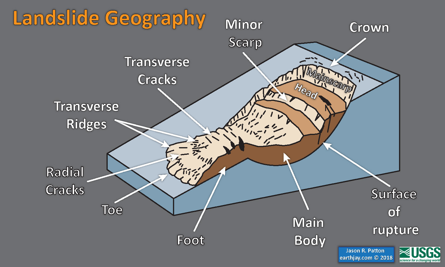
- Below is a diagram based upon a publication designed to educate the public about landslides and the processes that trigger them (USGS, 2004). Additional background information about landslide types can be found in Highland et al. (2008). There was a variety of landslide types that can be observed surrounding the earthquake region. So, this illustration can help people when they observing the landscape response to the earthquake whether they are using aerial imagery, photos in newspaper or website articles, or videos on social media. Will you be able to locate a landslide scarp or the toe of a landslide? This figure shows a rotational landslide, one where the land rotates along a curvilinear failure surface.
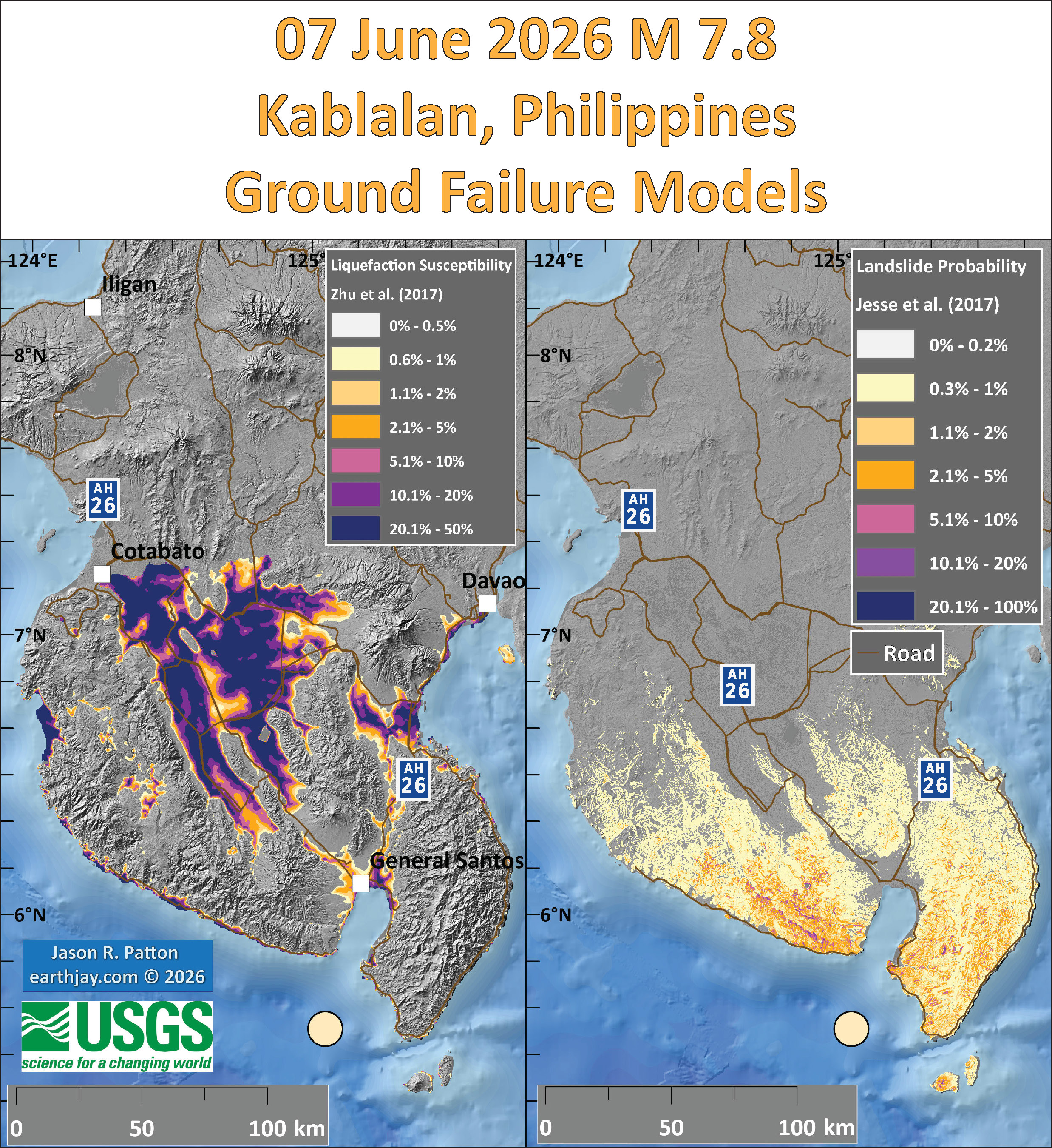
- Below is the liquefaction susceptibility and landslide probability map (Jessee et al., 2017; Zhu et al., 2017). Please head over to that report for more information about the USGS Ground Failure products (landslides and liquefaction). Basically, earthquakes shake the ground and this ground shaking can cause landslides.
- I use the same color scheme that the USGS uses on their website. Note how the areas that are more likely to have experienced earthquake induced liquefaction are in the valleys. Learn more about how the USGS prepares these model results here.
- There was an earthquake sequence in 2019. Sadly, I did not prepare an Earthquake Report for this sequence.
- These 2019 earthquakes (four M 6+ mainshocks) slipped along strike-slip crustal faults.
- Ferrario et al. (2019) mapped landslides that were triggered by these earthquakes (they also considered hydrologic triggering).
- These maps show the landslide number density and landslide area percentage for three time periods (earthquakes 3 & 4 happened in the same time period).
- Some more maps showing the frequency of landslides with different intensities.
- These plots show how the number of slides, landslide area, affected area, and landslide intensity all relate to earthquake magnitude.
- These data are compared to an existing dataset (Malamud et al., 2004).
@drwendyrocksit #Liquefaction is a process by which water-saturated sediment temporarily loses strength and acts as a fluid. This can happen during #earthquake shaking. #geophysics #geology ♬ Quicksand – Hatchie
This liquefaction experiment conducted by the Tokyo Geological Survey of Japan at the Disaster Prevention Exhibition in 2015, shows the effects of different foundations and how hollow objects such as water pipes come to the surface [source, full video: https://t.co/xYLjPY4IHZ] pic.twitter.com/r8LXtmvrO0
— Massimo (@Rainmaker1973) April 17, 2021
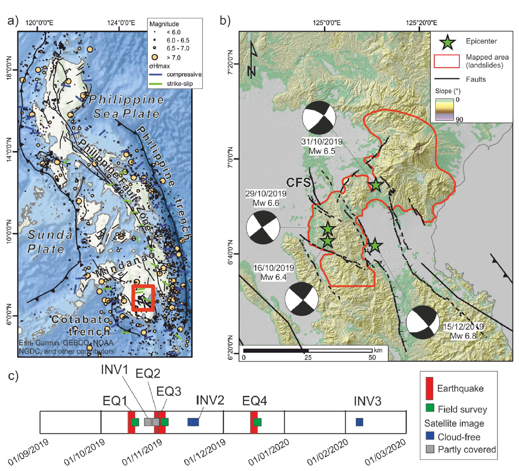
Tectonic setting of the study area. a sketch of the regional seismotectonic setting and historical seismicity, σHmax after Heidbach et al. (2018); b epicenter of the Mw > 6.0 events and mapped area (in red, i.e., the region where landslides have been mapped from satellite images); CFS: Cotabato fault system. Digital surface model AW3D30 (Jaxa) and derived slope map are shown in the background; c timeline showing the dates of analyzed satellite images and earthquakes (EQ: earthquake; INV: landslide inventory)
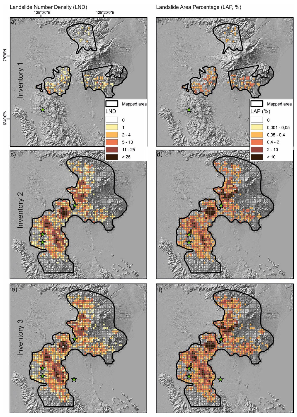
Landslide density and landslide area percentage for the three inventories.
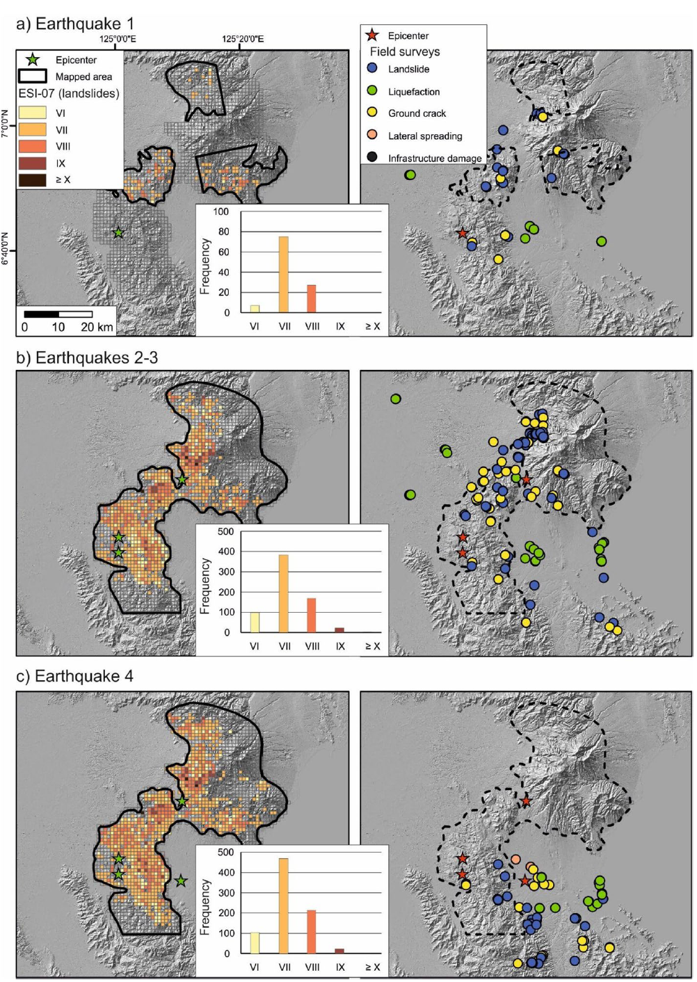
ESI-07 grid maps (left) and location of points surveyed in the field (right) after EQ1 (a), EQs 1–3 (b) and at the end of the sequence (c); for the left panels, histograms show the ESI-07 distribution of grid
cells.
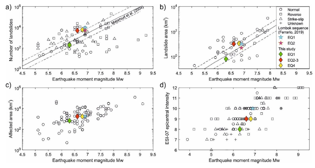
Comparison of the Cotabato–Davao del Sur sequence with global studies, including the multi-temporal inventory provided by Ferrario (2019) for the Lombok (Indonesia) seismic sequence. a the number of landslides vs MW, regression is after Malamud et al. (2004); b landslide area vs MW, regression is after
Malamud et al. (2004); c affected area vs MW; d ESI-07 epicentral intensity vs MW, dataset is after Ferrario et al. (2022)
Some Relevant Discussion and Figures
- Here is a tectonic map for this part of the world from Zahirovic et al., 2014. I left out all the acronym definitions (you’re welcome), but they are listed in the paper.
- Here are maps showing the regional tectonics (Smoczyk et al., 2013).
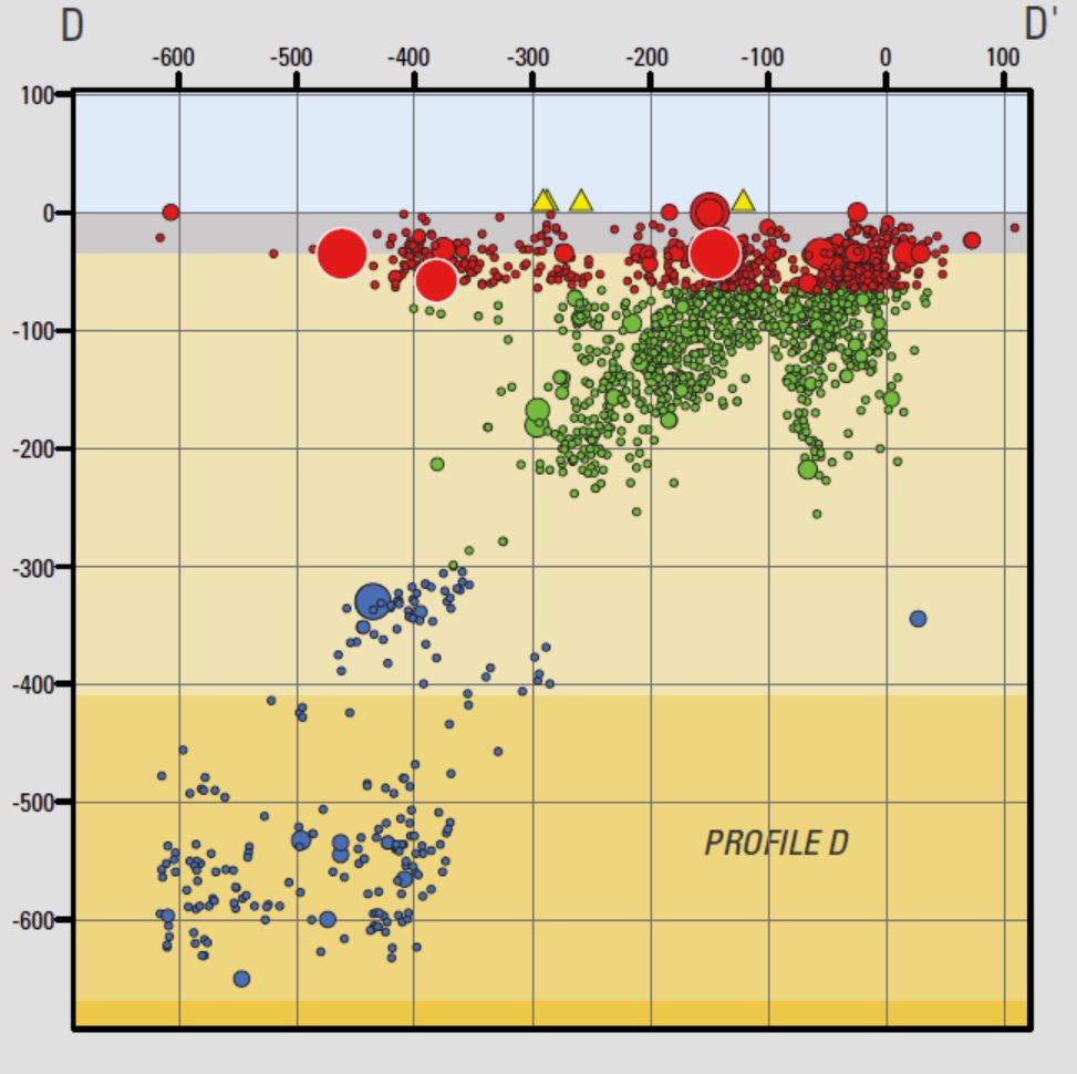
- Here is cross section D-D’ which is aligned perpendicular to the Cotabato trench.
- One may observe two subduction zones here. One is dipping to the west, with the top of the fault at the Philippines trench. The other megathrust fault is dipping to the east, associated with the Cotabato trench.
- This is one of my favorite figures of all time (Hall, 2011). Today’s earthquake sequence happened in the center of the middle panel, between the cyan (Molluca plate) and yellow plates. Read below for more details.
- Here are the figures from Zhang et al. (2017). First I present the tectonic overview figure, with captions below.
- Here is the seismic tomography profile figure.
- If we look at the first Zhang et al. (2017) figure above, the seismicity shows that the slab dipping to the west has earthquakes that extend much deeper than the zone dipping to the east. These authors hypothesized about why these subduciton zones are assymetrical (possibly due to mantle flow around the downgoing ocean crustal slabs). Zhang et al. (2017) conducted numerical analysis of mantle flow.
- Here is a figure that shows some illustrations depicting possible tectonic configurations for this region.
- Zhang et al., 2017 present below different possible configurations of double subduction zones.
- Based on their analyses, Zhang et al. (2017) make some conclusions about the divergent subduction zones in this region.
- The self-sustaining, asymmetrical subduction of the Molucca Sea plate may drive the convergence of the overriding plates and collision of magmatic arcs, even in an extensional setting of SE Asia.
- The earlier and faster subduction on the western Sangihe side with respect to the eastern Halmahera side predominantly led to formation of the present-day asymmetrical shape of the subducting Molucca Sea plate.
- The relative immobility of the western overriding Eurasian plate may have promoted the westward migration of the Halmahera arc in the Molucca Sea subduction zone.
- Bending of arcs was probably a consequence of the toroidal mantle flow induced by rollback of the subducting Molucca Sea plate on its both sides.
- DDS is unsustainable without effective escape of the slab-trapped mantle via toroidal flow. It is therefore likely that DDS is confined to narrow and short oceanic plates and is related to closure of archipelagic oceans and accretion of arcs in accretionary orogenic belts.
- Here is another tectonic map showing the Sorong fault and some splay faults (dashed lines running along Halmahera), one of which may be involved in today’s earthquake.
- Here is a map showing the major fault systems in the Philippines (Yumul et al., 2008).
- Here is a map showing the major fault systems and seismicity (color = depth) in the Philippines (Ramos et al., 2011).
- This shows Global Positioning System (GPS) velocities at various locations. These plate motions are represented as vectors in mm/yr. (see legend) Note that the plate motion vectors on either side of the Halmahera Strait are opposing each other, evidence of the contraction/convergence/compression across these plate boundary faults. Below I include the text from the original figure caption in blockquote.
- Here is a summary map showing estimates of plate convergence from Ohkura et al., 2015.

Regional tectonic setting with plate boundaries (MORs/transforms = black, subduction zones = teethed red) from Bird (2003) and ophiolite belts representing sutures modified from Hutchison (1975) and Baldwin et al. (2012). West Sulawesi basalts are from Polvé et al. (1997), fracture zones are from Matthews et al. (2011) and basin outlines are from Hearn et al. (2003).

Along its western margin, the Philippine Sea plate is associated with a zone of oblique convergence with the Sunda plate. This highly active convergent plate boundary extends along both sides the Philippine Islands, from Luzon in the north to Sulawesi in the south. The tectonic setting of the Philippines is unusual in several respects: it is characterized by opposite-facing subduction systems on its east and west sides; the archipelago is cut by a major transform fault, the Philippine Fault; and the arc complex itself is marked by volcanism, faulting, and high seismic activity. Subduction of the Philippine Sea plate occurs at the eastern margin of the archipelago along the Philippine Trench and its northern extension, the East Luzon Trough. The East Luzon Trough is thought to be an unusual example of a subduction zone in the process of formation, as the Philippine Trench system gradually extends northward (Hamburger and others, 1983).

3D cartoon of plate boundaries in the Molucca Sea region modified from Hall et al. (1995). Although seismicity identifies a number of plates there are no continuous boundaries, and the Cotobato, North Sulawesi and Philippine Trenches are all intraplate features. The apparent distinction between different crust types, such as Australian continental crust and oceanic crust of the Philippine and Molucca Sea, is partly a boundary inactive since the Early Miocene (east Sulawesi) and partly a younger but now probably inactive boundary of the Sorong Fault. The upper crust of this entire region is deforming in a much more continuous way than suggested by this cartoon.

(a) Sketch of the Molucca Sea subduction zone and its vicinity. (b) Cross section (A-B) demonstrating the structure of arc-arc collision zone (modified after Hall and Smyth [2008]). (c) Distribution of earthquake events (2011.1.1–2015.12.31) and focal mechanism; the insert shows the vertical profile of epicenters sliced at position B-B0 . The black
dashed line in Figure 1a is the position of cross section A-B in Figure 1b, and the red solid lines in Figure 1c are the cross sections of the seismic tomographic velocity model in Figure 2.

Vertical slices of seismic velocity beneath the Molucca Sea and its surrounding regions, in which positive velocity anomalies outline the unique shape of the subducting Molucca Sea plate. The tomographic images are sliced from the global P wave velocity anomaly model UU-P07 [Amaru, 2007] along positions shown in Figure 1c.

Cartoon of end-member models illustrating effects of the order of subduction initiation, the mobility and thickness of the overriding plates on slab morphology, and migration of the overriding plates during DDS. Idealized DDS features (a) symmetrical subduction of slabs and (b–d) asymmetrical plate shape resulted from influence of order of subduction initiation, mobility, and thickness of overriding plates, respectively. (e) Tentative interpretation of formation of the asymmetrical DDS observed in the Molucca Sea region. Size of arrows indicate relative scale of the subduction-induced mantle flow.
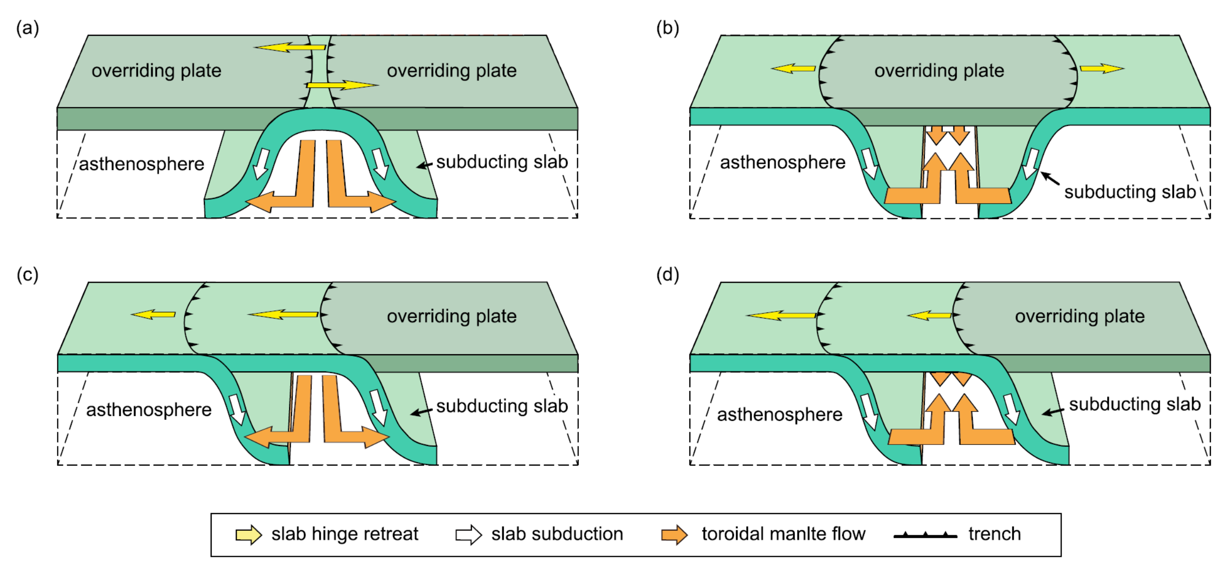
Cartoons illustrating several forms of double subduction. (a) Divergent double subduction (descripted in this study and by Soesoo et al. [1997], Di Leo et al. [2014], Li et al., [2014], etc.). (b) Double subduction with opposite dipping directions (descripted by Maruyama et al. [ 2007]). (c and d) Convergent double subduction (descripted by Jagoutz et al. [2015] and Billen [2015]). In all of these case, sustainable subduction of the oceanic plate(s) requires smooth escape (Figures 17a and 17c) of the slab-trapped mantle or replenishment of external materials of mantle into the void space left by slab rollback (Figures 17b and 17d). The toroidal mantle flow (orange arrows) plays a dominant role in
redistribution of material during all these types of double subduction.

Location map and active faults of the Molucca Sea region. Fault colours: blue, convergence; red, transvergence; yellow, divergence; grey, uncertain motion. Fault abbreviations: CF, Catabato Fault; GF, Gorontalo Fault; NST, North Sulawesi Trench; PKF, Palu-Koro Fault; SF, Sorong Fault.
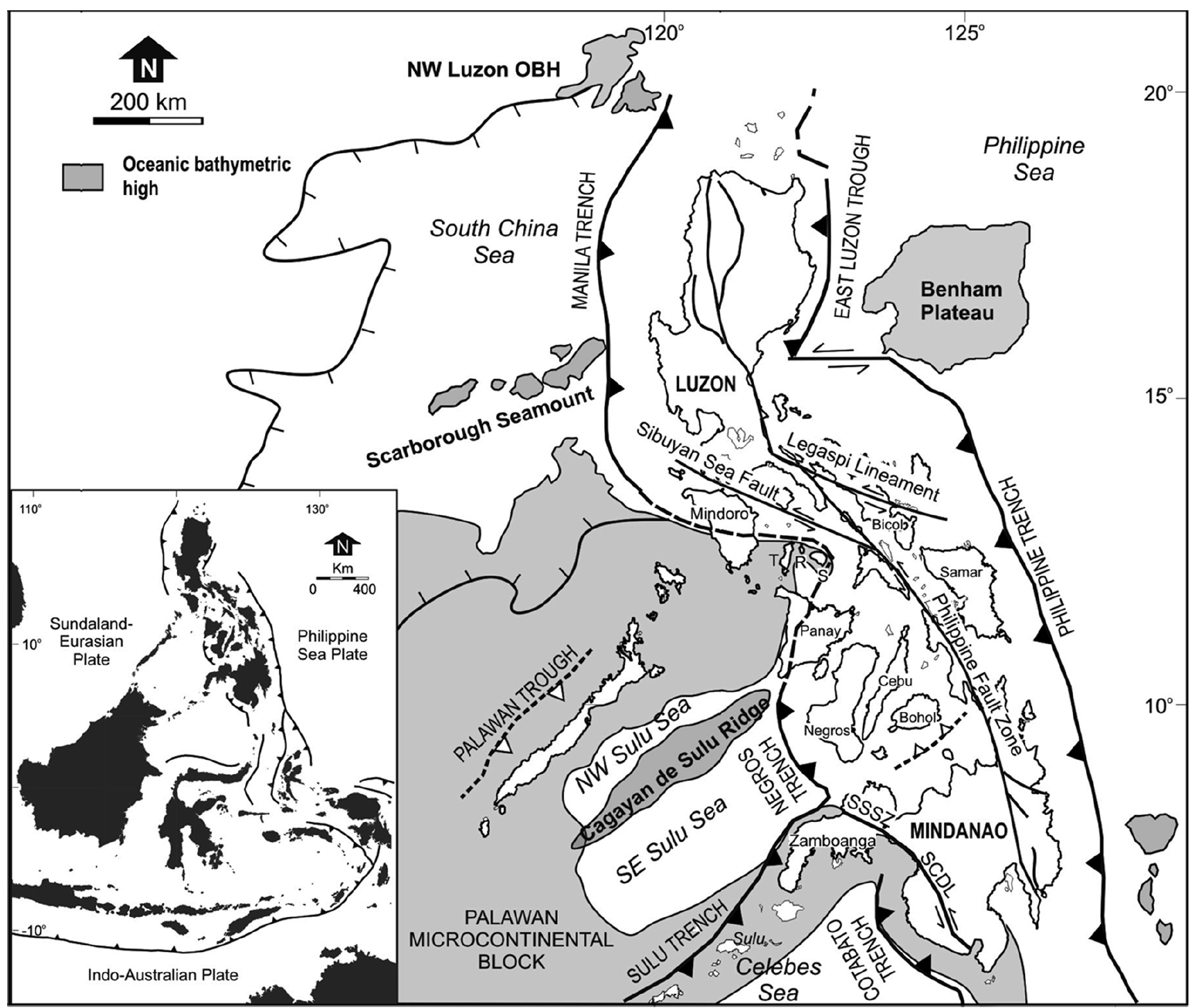
The Philippine island arc system is surrounded by trenches, marginal basins and oceanic bathymetric highs (OBH). Moreover, the entire length of the archipelago is traversed by the left-lateral Philippine Fault Zone and some of its significant splays. Dashed line with open triangle corresponds to the proto-Southeast Bohol Trench. Inset shows the three major plates that bound the Philippine archipelago – Sundaland-Eurasian, Philippine Sea and the Indo-Australian plates. See text for discussion. SSSZ = Siayan-Sindangan Suture Zone; SCDL= Sindangan-Cotabato- Daguma Lineament, T = Tablas, R = Romblon and S = Sibuyan.
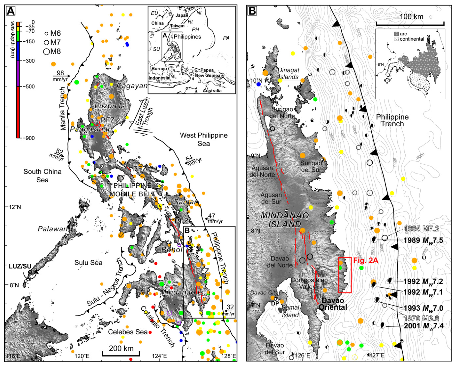
Seismotectonic setting of Davao Oriental, Philippines. (A) Map showing tectonic structures and seismicity of the archipelago. Convergence rates along subduction zones are shown with the Luzon/Sunda block (LUZ/SU) rotation pole (Rangin et al., 1999). Seismicity (M > 6) (1897–2008) are from the Philippine Institute of Volcanology and Seismology (PHIVOLCS) database while active faults (bold solid lines) of the Philippine fault zone (PFZ) are from Tsutsumi and Perez (2010). Topographic data are from the Shuttle Radar Topography Mission (SRTM) (Farr et al., 2007). The rectangle shows the location of B. Inset shows surrounding tectonic elements and location of the Philippines in the western Pacific: EU – Eurasian plate, SU – Sunda block, PH – Philippine Sea plate, PA – Pacific plate, Nt – Nankai trough, Rt – Ryukyu trench. (B) Seismicity and active structures nearby the study area (rectangle). Large historical earthquakes (1608–1895) (hollow circles) are from Bautista and Oike (2000), focal mechanism solutions (M > 6) (1976–2010) are from the Global Centroid Moment Tensor (CMT) Catalog, and bathymetry are from the National Geophysical Data Center (NGDC) (Amante and Eakins, 2009). Inset shows the basement rocks of Mindanao Island. Dashed lines show provincial boundaries. DP: Davao port tide gauge station.

Topographic and tectonic map of the Indonesian archipelago and surrounding region. Labeled, shaded arrows show motion (NUVEL-1A model) of the first-named tectonic plate relative to the second. Solid arrows are velocity vectors derived from GPS surveys from 1991 through 2001, in ITRF2000. For clarity, only a few of the vectors for Sumatra are included. The detailed velocity field for Sumatra is shown in Figure 5. Velocity vector ellipses indicate 2-D 95% confidence levels based on the formal (white noise only) uncertainty estimates. NGT, ew Guinea Trench; NST, North Sulawesi Trench; SF, Sumatran Fault; TAF, Tarera-Aiduna Fault. Bathymetry [Smith and Sandwell, 1997] in this and all subsequent figures contoured at 2 km intervals
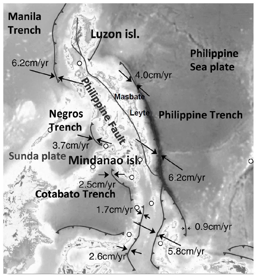
Tectonic map of the Philippines and surrounding areas. Convergence rates of each subduction zone, obtained from GPS station (shown as white circles) velocities, are from Tabei et al. (2008)
Seismic Hazard and Seismic Risk
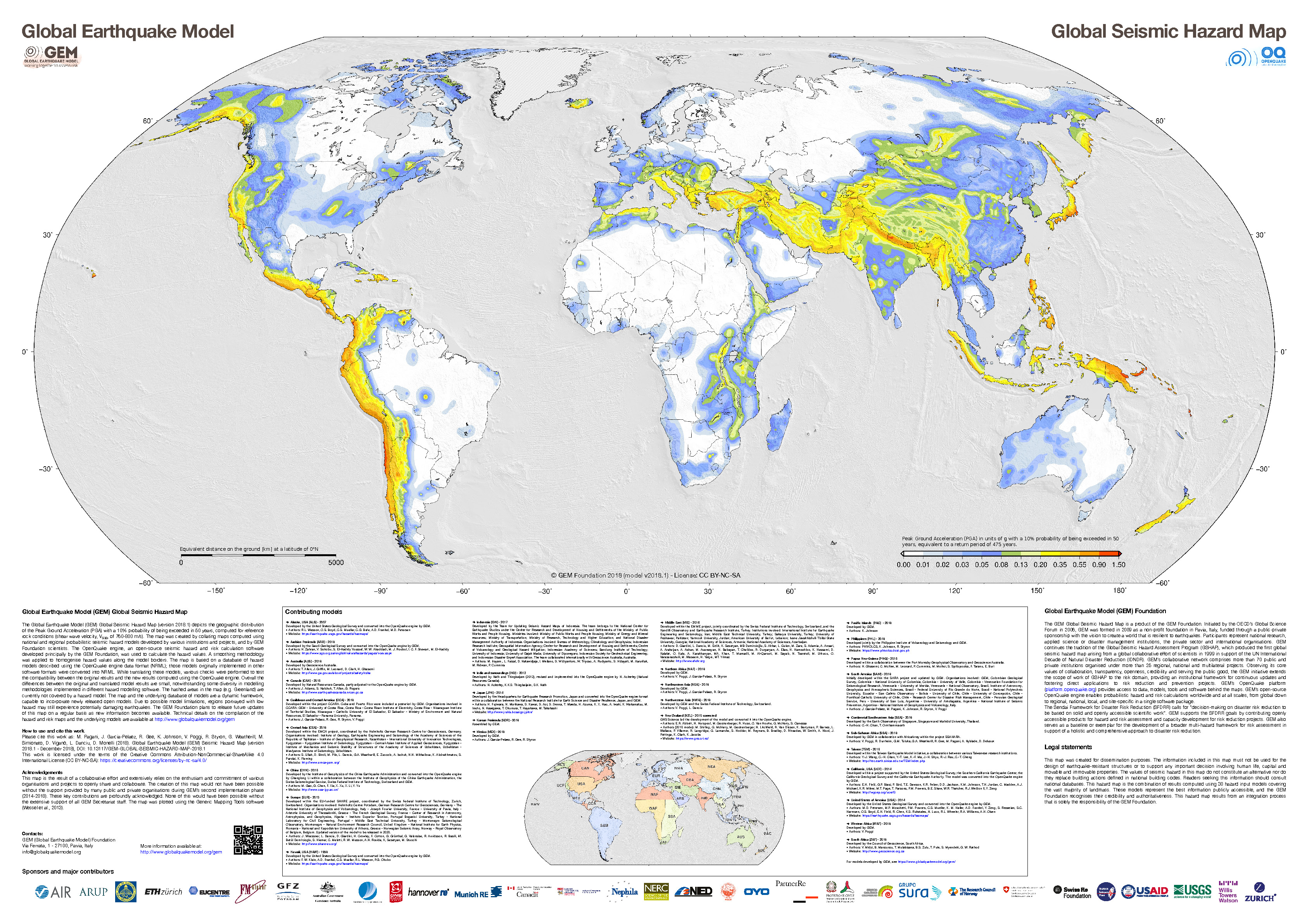
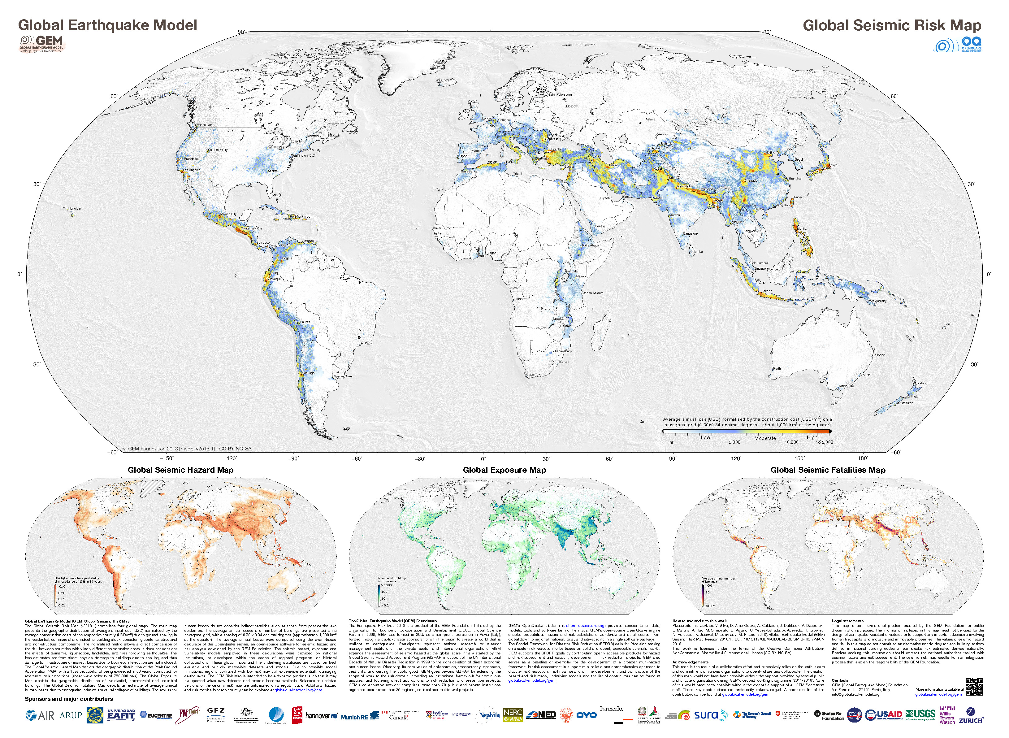
- These are the two maps shown in the map above, the GEM Seismic Hazard and the GEM Seismic Risk maps from Pagani et al. (2018) and Silva et al. (2018).
- The GEM Seismic Hazard Map:
- The Global Earthquake Model (GEM) Global Seismic Hazard Map (version 2018.1) depicts the geographic distribution of the Peak Ground Acceleration (PGA) with a 10% probability of being exceeded in 50 years, computed for reference rock conditions (shear wave velocity, VS30, of 760-800 m/s). The map was created by collating maps computed using national and regional probabilistic seismic hazard models developed by various institutions and projects, and by GEM Foundation scientists. The OpenQuake engine, an open-source seismic hazard and risk calculation software developed principally by the GEM Foundation, was used to calculate the hazard values. A smoothing methodology was applied to homogenise hazard values along the model borders. The map is based on a database of hazard models described using the OpenQuake engine data format (NRML). Due to possible model limitations, regions portrayed with low hazard may still experience potentially damaging earthquakes.
- Here is a view of the GEM seismic hazard map for Indonesia.
- The USGS Seismic Hazard Map:
- Here is another version of the seismic hazard for this region (Smoczyk et al., 2013). The GEM map suggests that the islands along the Halmahera Strait may have accelerations between 0.8-1.6 m2. This translates to 0.08 to 0.16 g. The GEM seismic hazard map shows a potential shaking of 0.20-0.35 g, slightly higher.
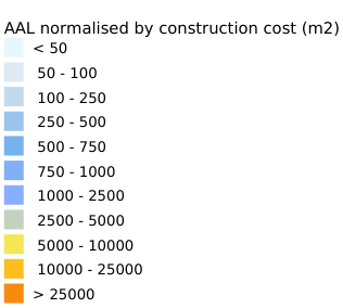
- The GEM Seismic Risk Map:
- The Global Seismic Risk Map (v2018.1) presents the geographic distribution of average annual loss (USD) normalised by the average construction costs of the respective country (USD/m2) due to ground shaking in the residential, commercial and industrial building stock, considering contents, structural and non-structural components. The normalised metric allows a direct comparison of the risk between countries with widely different construction costs. It does not consider the effects of tsunamis, liquefaction, landslides, and fires following earthquakes. The loss estimates are from direct physical damage to buildings due to shaking, and thus damage to infrastructure or indirect losses due to business interruption are not included. The average annual losses are presented on a hexagonal grid, with a spacing of 0.30 x 0.34 decimal degrees (approximately 1,000 km2 at the equator). The average annual losses were computed using the event-based calculator of the OpenQuake engine, an open-source software for seismic hazard and risk analysis developed by the GEM Foundation. The seismic hazard, exposure and vulnerability models employed in these calculations were provided by national institutions, or developed within the scope of regional programs or bilateral collaborations.


- 2026.06.07 M 7.8 Philippines 355
- 2026.04.01 M 7.4 Halmahera 348
- 2025.09.30 M 6.9 Philippines POSTER
- 2024.08.02 M 6.8 Philippines (poster)
- 2024.07.11 M 7.1 Philippines
- 2023.12.02 M 7.6 Philippines
- 2022.07.27 M 7.0 Philippines (poster)
- 2021.08.11 M 7.1 Philippines (poster)
- 2019.11.14 M 7.1 Halmahera
- 2019.07.14 M 7.3 Halmahera
- 2018.12.29 M 7.0 Philippines
- 2017.12.08 M 6.5 Caroline Ridge
- 2017.12.09 M 6.5 Caroline Ridge Update #1
- 2017.08.11 M 6.2 Philippines
- 2017.04.28 M 6.9 Philippines
- 2017.04.08 M 5.9 Philippines
- 2017.01.10 M 7.3 Celebes Sea
- 2016.07.29 M 7.7 Mariana
- 2015.03.17 M 6.2 Molucca Sea
- 2014.11.26 M 6.8 Molucca Sea
- 2014.11.21 M 6.5 Molucca Sea
- 2014.11.15 M 7.1 Molucca Sea
Philippines | Western Pacific
Earthquake Reports
Social Media
- Frisch, W., Meschede, M., Blakey, R., 2011. Plate Tectonics, Springer-Verlag, London, 213 pp.
- Hayes, G., 2018, Slab2 – A Comprehensive Subduction Zone Geometry Model: U.S. Geological Survey data release, https://doi.org/10.5066/F7PV6JNV.
- Holt, W. E., C. Kreemer, A. J. Haines, L. Estey, C. Meertens, G. Blewitt, and D. Lavallee (2005), Project helps constrain continental dynamics and seismic hazards, Eos Trans. AGU, 86(41), 383–387, , https://doi.org/10.1029/2005EO410002. /li>
- Jessee, M.A.N., Hamburger, M. W., Allstadt, K., Wald, D. J., Robeson, S. M., Tanyas, H., et al. (2018). A global empirical model for near-real-time assessment of seismically induced landslides. Journal of Geophysical Research: Earth Surface, 123, 1835–1859. https://doi.org/10.1029/2017JF004494
- Kreemer, C., J. Haines, W. Holt, G. Blewitt, and D. Lavallee (2000), On the determination of a global strain rate model, Geophys. J. Int., 52(10), 765–770.
- Kreemer, C., W. E. Holt, and A. J. Haines (2003), An integrated global model of present-day plate motions and plate boundary deformation, Geophys. J. Int., 154(1), 8–34, , https://doi.org/10.1046/j.1365-246X.2003.01917.x.
- Kreemer, C., G. Blewitt, E.C. Klein, 2014. A geodetic plate motion and Global Strain Rate Model in Geochemistry, Geophysics, Geosystems, v. 15, p. 3849-3889, https://doi.org/10.1002/2014GC005407.
- Meyer, B., Saltus, R., Chulliat, a., 2017. EMAG2: Earth Magnetic Anomaly Grid (2-arc-minute resolution) Version 3. National Centers for Environmental Information, NOAA. Model. https://doi.org/10.7289/V5H70CVX
- Müller, R.D., Sdrolias, M., Gaina, C. and Roest, W.R., 2008, Age spreading rates and spreading asymmetry of the world’s ocean crust in Geochemistry, Geophysics, Geosystems, 9, Q04006, https://doi.org/10.1029/2007GC001743
- Pagani,M. , J. Garcia-Pelaez, R. Gee, K. Johnson, V. Poggi, R. Styron, G. Weatherill, M. Simionato, D. Viganò, L. Danciu, D. Monelli (2018). Global Earthquake Model (GEM) Seismic Hazard Map (version 2018.1 – December 2018), DOI: 10.13117/GEM-GLOBAL-SEISMIC-HAZARD-MAP-2018.1
- Silva, V ., D Amo-Oduro, A Calderon, J Dabbeek, V Despotaki, L Martins, A Rao, M Simionato, D Viganò, C Yepes, A Acevedo, N Horspool, H Crowley, K Jaiswal, M Journeay, M Pittore, 2018. Global Earthquake Model (GEM) Seismic Risk Map (version 2018.1). https://doi.org/10.13117/GEM-GLOBAL-SEISMIC-RISK-MAP-2018.1
- Storchak, D. A., D. Di Giacomo, I. Bondár, E. R. Engdahl, J. Harris, W. H. K. Lee, A. Villaseñor, and P. Bormann (2013), Public release of the ISC-GEM global instrumental earthquake catalogue (1900–2009), Seismol. Res. Lett., 84(5), 810–815, doi:10.1785/0220130034.
- Zhu, J., Baise, L. G., Thompson, E. M., 2017, An Updated Geospatial Liquefaction Model for Global Application, Bulletin of the Seismological Society of America, 107, p 1365-1385, https://doi.org/0.1785/0120160198
- Hall, R., 2011. Australia-SE Asia collision: plate tectonics and crustal flow in Geological Society, London, Special Publications 2011; v. 355; p. 75-109 doi: 10.1144/SP355.5
- Hall., R., Audley-Charles, M.G., Banner, F.T., Hidayat, S., Tobing, S.L., 1988. Basement rocks of the Halmahera region, eastern Indonesia: a Late Cretaceous-early Tertiary arc and fore-arc in Journal of the Geological Society, v. 145, p. 65-84
- Horspool, N., Pranantyo, I., Griffin, J., Latief, H., Natawidjaja, D. H., Kongko, W., Cipta, A., Bustaman, B., Anugrah, S. D., and Thio, H. K., 2014. A probabilistic tsunami hazard assessment for Indonesia, Nat. Hazards Earth Syst. Sci., 14, 3105-3122, https://doi.org/10.5194/nhess-14-3105-2014, 2014.
- McCaffrey, R., Silver, E.A., and Raitt, R.W., 1980. Crustal Structure of the Molucca Sea Collision Zone, Indonesia in The Tectonic and Geologic Evolution of Southeast Asian Seas and Islands-Geophysical Monograph 23, p. 161-177.
- Pagani,M. , J. Garcia-Pelaez, R. Gee, K. Johnson, V. Poggi, R. Styron, G. Weatherill, M. Simionato, D. Viganò, L. Danciu, D. Monelli (2018). Global Earthquake Model (GEM) Seismic Hazard Map (version 2018.1 – December 2018), DOI: 10.13117/GEM-GLOBAL-SEISMIC-HAZARD-MAP-2018.1
- Silva, V ., D Amo-Oduro, A Calderon, J Dabbeek, V Despotaki, L Martins, A Rao, M Simionato, D Viganò, C Yepes, A Acevedo, N Horspool, H Crowley, K Jaiswal, M Journeay, M Pittore, 2018. Global Earthquake Model (GEM) Seismic Risk Map (version 2018.1). https://doi.org/10.13117/GEM-GLOBAL-SEISMIC-RISK-MAP-2018.1
- Smoczyk, G.M., Hayes, G.P., Hamburger, M.W., Benz, H.M., Villaseñor, Antonio, and Furlong, K.P., 2013. Seismicity of the Earth 1900–2012 Philippine Sea plate and vicinity: U.S. Geological Survey Open-File Report 2010–1083-M, 1 sheet, scale 1:10,000,000.
- Zahirovic et al., 2014. The Cretaceous and Cenozoic tectonic evolution of Southeast Asia in Solid Earth, v. 5, p. 227-273, doi:10.5194/se-5-227-2014.
- Zhang, Q., F. Guo, L. Zhao, and Y. Wu, 2017. Geodynamics of divergent double subduction: 3-D numerical modeling of a Cenozoic example in the Molucca Sea region, Indonesia, J. Geophys. Res. Solid Earth, 122, 3977–3998, doi:10.1002/2017JB013991.
- Zulkifli, M., Rudyanto, A., and Sakti, A.P., 2016. The View of Seismic Hazard in The Halmahera Region in proceedings from International Symposium on Earth Hazard and Disaster Mitigation (ISEDM) 2016 AIP Conf. Proc. 1857, 050004-1–050004-7; doi:10.1063/1.4987082
References:
Basic & General References
Specific References
Return to the Earthquake Reports page.
- Sorted by Magnitude
- Sorted by Year
- Sorted by Day of the Year
- Sorted By Region