Stand By: Earthquake Report in Progress ;-)
A few weeks ago there was a magnitude M 7.1 earthquake to the southwest of today’s M 6.8 earthquake. I will describe both earthquakes a bit here.
11 July 2024 M 7.1:
https://earthquake.usgs.gov/earthquakes/eventpage/us7000myfa/executive
2 August 2024 M 6.8:
https://earthquake.usgs.gov/earthquakes/eventpage/us6000nhqc/executive
Here is a view of the tectonic plates in this region.
- This is the low-angle oblique view of the region (Hall, 2011).
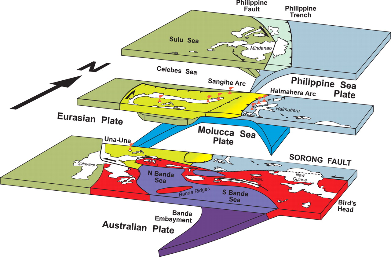
3D cartoon of plate boundaries in the Molucca Sea region modified from Hall et al. (1995). Although seismicity identifies a number of plates there are no continuous boundaries, and the Cotobato, North Sulawesi and Philippine Trenches are all intraplate features. The apparent distinction between different crust types, such as Australian continental crust and oceanic crust of the Philippine and Molucca Sea, is partly a boundary inactive since the Early Miocene (east Sulawesi) and partly a younger but now probably inactive boundary of the Sorong Fault. The upper crust of this entire region is deforming in a much more continuous way than suggested by this cartoon.
In July there was a deep earthquake offshore of the Philippines.
The M 7.1 earthquake (lindol) has a hypocentral depth of ~630 km. The USGS Slab 2.0 (Hayes et al., 2012) depth at this location is about 570 km.
The earthquake appears to be within the subducted plate. The earthquake has a normal mechanism (the moment tensor) which represents that there is extension in this plate (common for this tectonic setting).
Here is an earthquake that happened in almost the same place: 2017.01.10 M 7.3 Celebes Sea
Learn more about deep earthquakes in this report: 2018.04.02 M 6.8 Bolivia
In this part of the world, there is an oceanic feature called the Halmahera Strait (aka the Molucca Sea), a north-south passageway south of the island of Mindanao, Philippines.
Either side of the strait is lined with islands formed as a part of magmatic arcs (volcanic arcs). These volcanic chains are there because there are subduction zones on either side of Halmahera Strait.
On the western side of the strait, the Molucca Sea plate subducts down to the west beneath the Sunda plate (in the Celebes Sea). Cao et al (2021) may call this the South China Sea plate(?).
On the eastern side of the strait, the same Molucca Sea plate subducts down to the east beneath the Philippine Sea plate (or a small block within this plate).
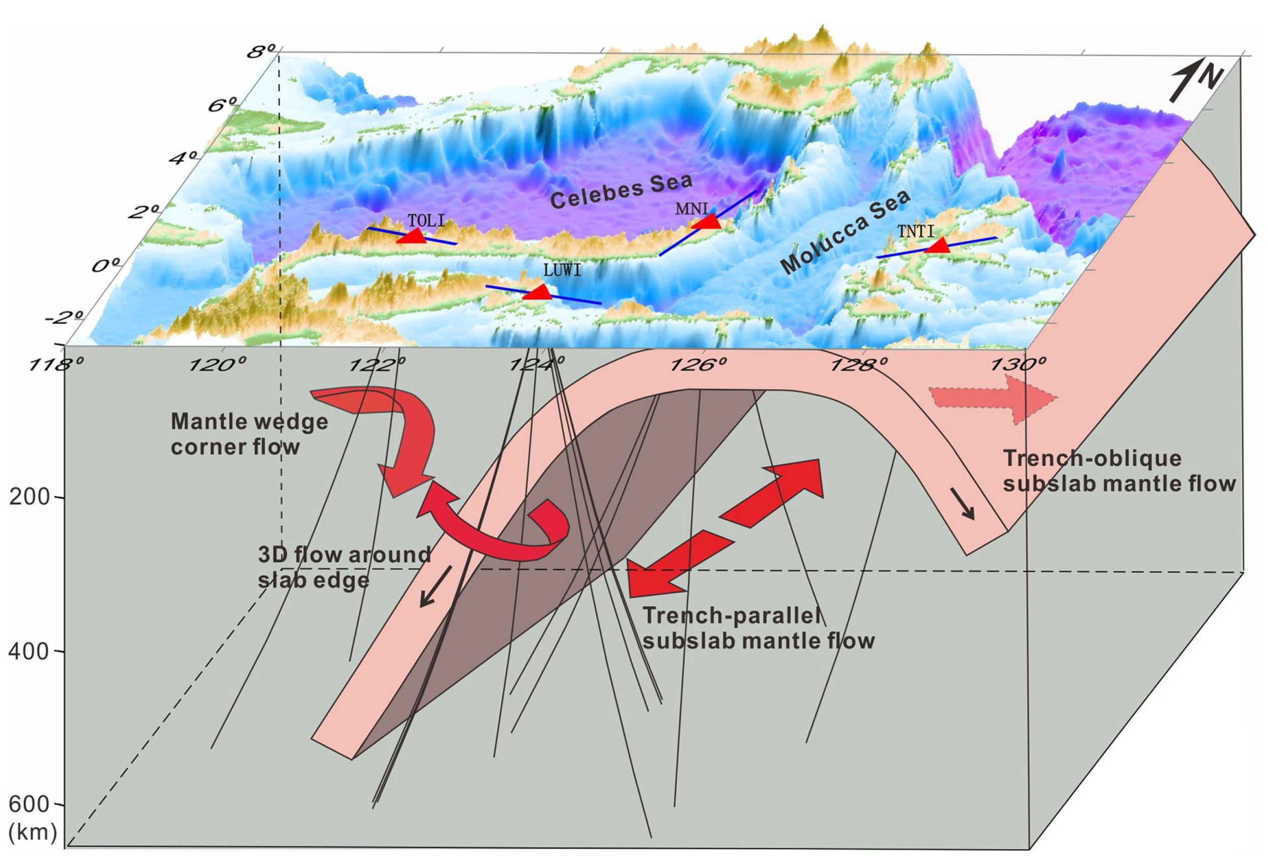
Here is a diagram from Cao et al. (2021) that shows how these two subduction zones are geometrically oriented. I include this and other figures, with their captions, further down in the report.
Today’s M 6.8 earthquake happened in a different tectonic setting.
The 2 August 2024 M 6.8 earthquake has a reverse mechanism, a result of compression.
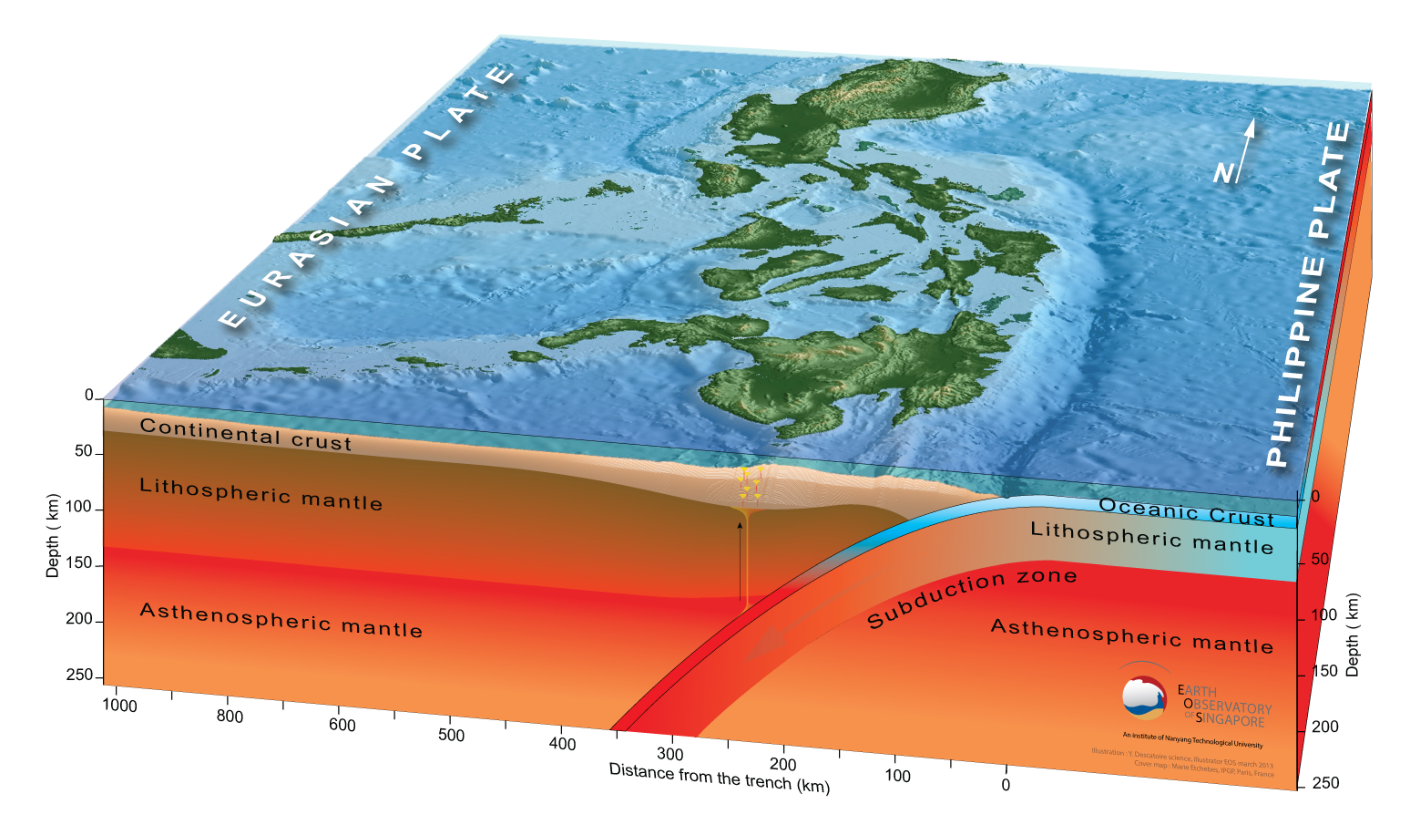
This part of the Philippines is dominated by the convergent plate margin, a megathrust subduction zone. This subduction zone forms the Philippines trench.
This plate boundary is formed by the subduction of the Philippine Sea plate from the east, downwards beneath the complicated series of plates and microplates that form the archipelago of the Philippines (the main plate to the west is the Sunda plate, part of Eurasia).
On 2 December 2023, there was a M 7.6 earthquake near today’s M 6.8. It is not immediately clear if this M 6.8 was on the megathrust interface. So, it may be that the M 6.8 was within the upper plate (so was triggered by the M 7.6). Some may call the M 6.8 an aftershock, some may consider it a triggered earthquake.
Here is a block diagram showing the tectonic plate boundaries (from Earth Observatory Singapore). Another great illustration is from Hall, further down in the report.
Additional information for this region can be found in the Earthquake Report for the mainshock earthquake in this sequence, the 2 December 2023 magnitude M 7.6 gempa/earthquake.
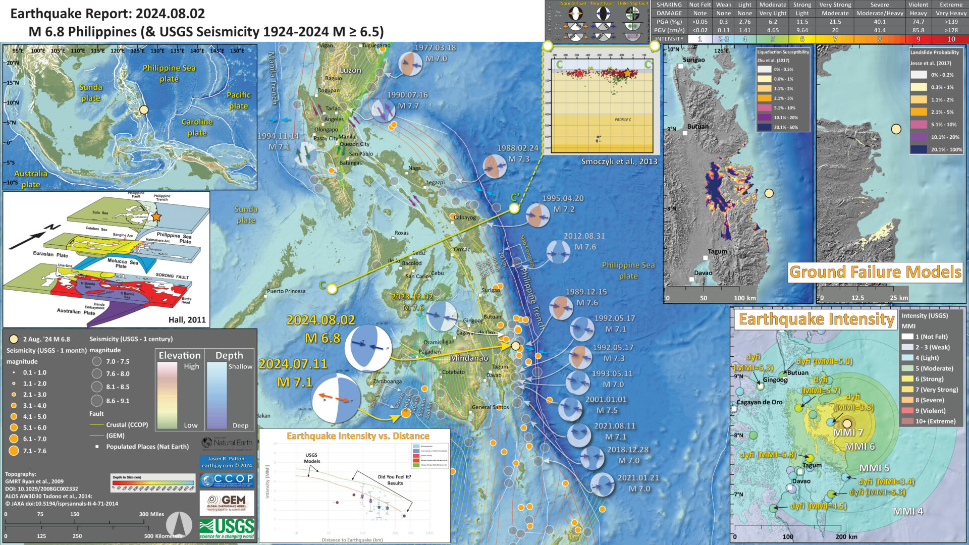
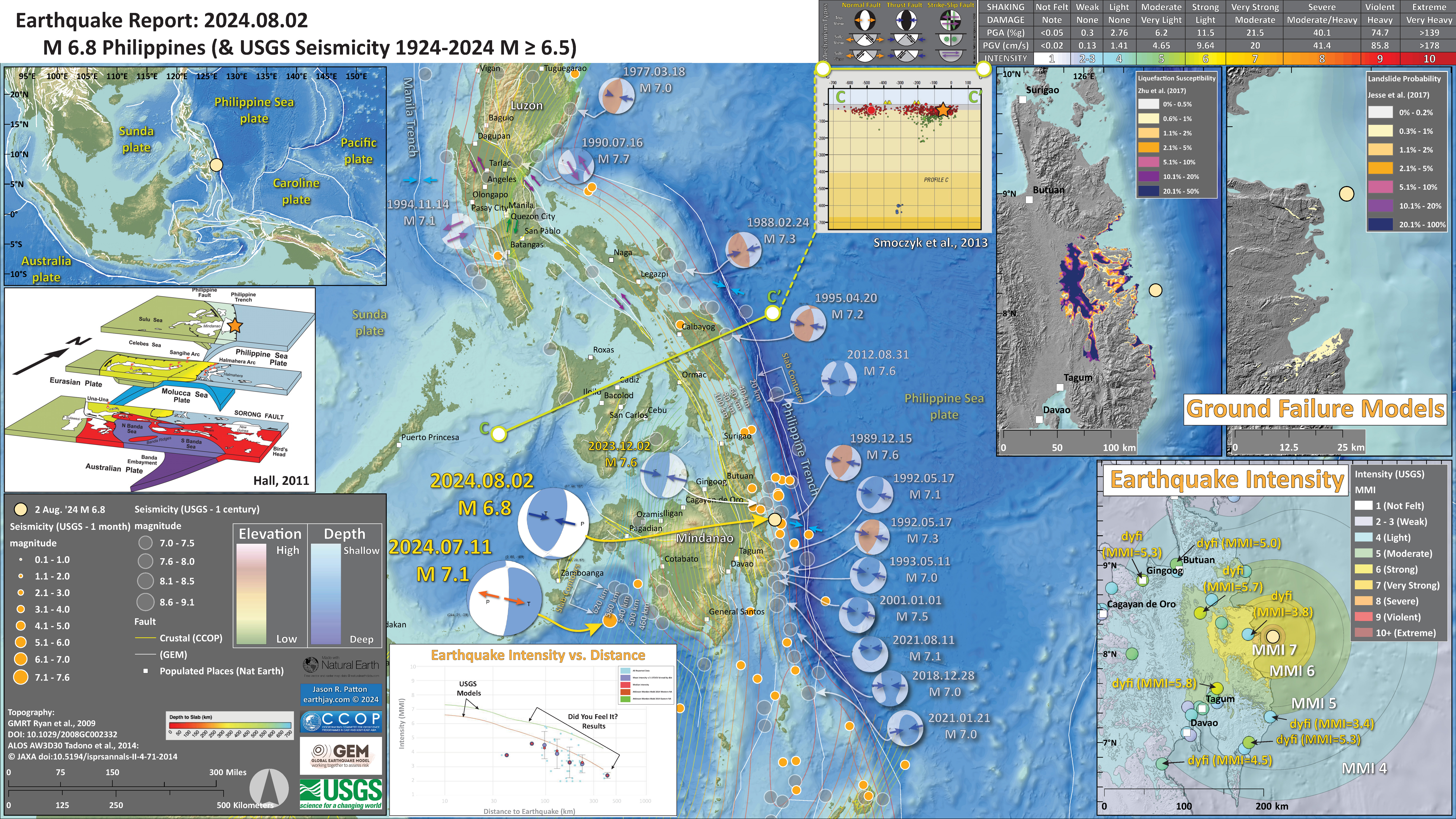
Below is my interpretive poster for this earthquake
- I plot the seismicity from the past month, with diameter representing magnitude (see legend). I include earthquake epicenters from 1923-2023 with magnitudes M ≥ 3.0 in one version.
- I plot the USGS fault plane solutions (moment tensors in blue and focal mechanisms in orange), possibly in addition to some relevant historic earthquakes.
- A review of the basic base map variations and data that I use for the interpretive posters can be found on the Earthquake Reports page. I have improved these posters over time and some of this background information applies to the older posters.
- Some basic fundamentals of earthquake geology and plate tectonics can be found on the Earthquake Plate Tectonic Fundamentals page.
- In the upper left corner is a map showing the plate tectonic boundaries (from the GEM).
- Below the tectonic map is a low angle oblique view of the plate boundaries showing the subsurface geometry of the subduction zones (Hall, 2011). I placed an orange star in the location of the M 6.8.
- In the lower right corner is a map that shows the M 6.8 earthquake intensity using the modified Mercalli intensity scale. Earthquake intensity is a measure of how strongly the Earth shakes during an earthquake, so gets smaller the further away one is from the earthquake epicenter. The map colors represent a model of what the intensity may be. The USGS has a system called “Did You Feel It?” (DYFI) where people enter their observations from the earthquake and the USGS calculates what the intensity was for that person. The dots with yellow labels show what people actually felt in those different locations.
- In the lower left center is a plot that shows the same intensity (both modeled and reported) data as displayed on the map. Note how the intensity gets smaller with distance from the earthquake.
- In the upper right corner are two maps showing the possibility of earthquake induced liquefaction for these two earthquakes. I discuss these phenomena in more detail later in the report.
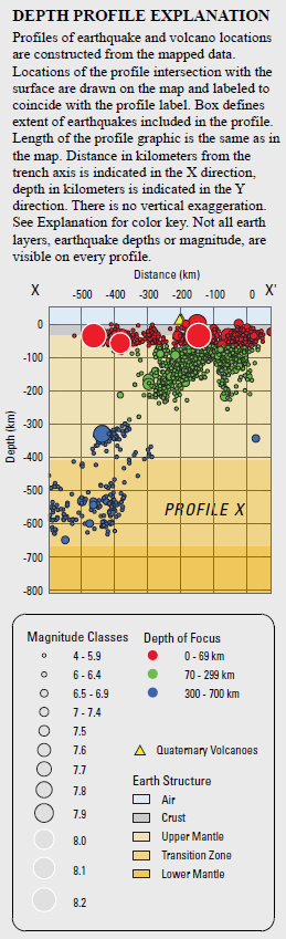
- To the left of the ground failure maps is a cross section showing the seismicity of the region along profile C-C’ (Smoczyk et al., 2013). Note how we can see the Philippine Sea plate seismicity diving downwards to the west. The Philippine trench is located at 0 km on the horizontal axis. The M 6.8 earthquake is projected onto this cross section.
I include some inset figures.
- Here is the map with a month’s seismicity plotted.
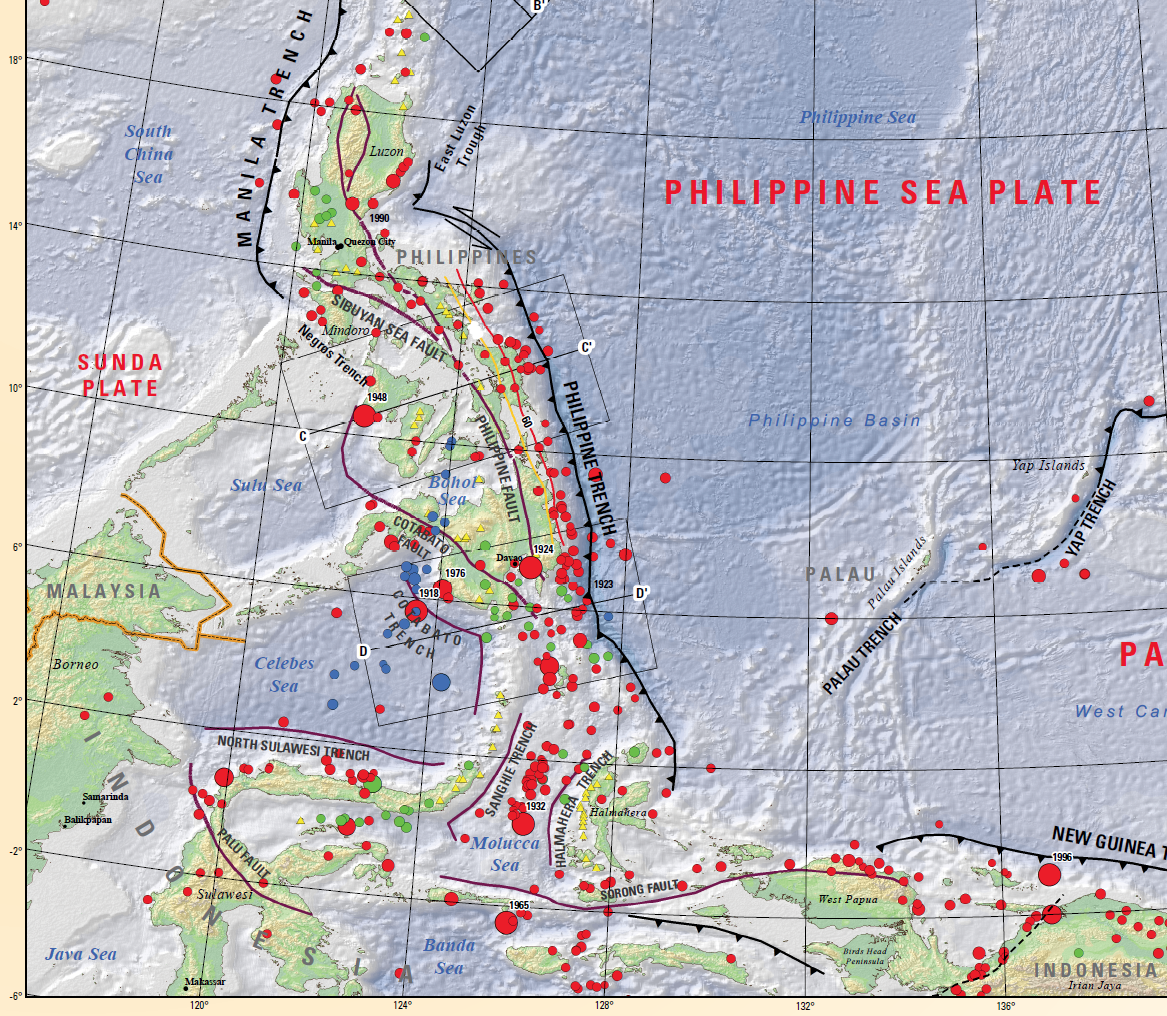
The USGS Maps and Cross-Sections
- Here is the map from Smocyk et al., 2013, followed by the legend. The entire poster is here (92 MB pdf).
- Below are two cross sections that show the subduction zone seismicity, followed by the legend. The location of these cross sections are labeled on the map above.
- This map shows the seismic hazard for this region. The color represents the likelihood of any region experiencing ground shaking of a particular magnitude. The scale is “Peak Ground Acceleration.” Units are m/s^2. Purple represents gravitational acceleration of 1 g, gravity at Earth’s surface.


Tectonic Background: 11 July 2024 M 7.1 Normal faulting earthquake
- Here is the tectonic map from Cao et al. (2013).
- Cross Section A-A’ is the general location of the low angle oblique view of these plates in a figure below.
- Cao et al. (2021) used advanced methods to process seismic waves to interrogate the subsurface. This figure shows the results from their modeling.
- Cross section E-E’ is in the region near the 11 July 2024 M 7.1 normal fault earthquake. Cross section C-C’ is in the general region depicted by the low angle oblique view in the next figure below.
- Here is the low angle oblique view of the tectonic plates in this region.
- Here are the figures from Zhang et al. (2017). First I present the tectonic overview figure, with captions below.
- Here is the seismic tomography profile figure.
- If we look at the first Zhang et al. (2017) figure above, the seismicity shows that the slab dipping to the west has earthquakes that extend much deeper than the zone dipping to the east. These authors hypothesized about why these subduciton zones are assymetrical (possibly due to mantle flow around the downgoing ocean crustal slabs). Zhang et al. (2017) conducted numerical analysis of mantle flow.
- Here is a figure that shows some illustrations depicting possible tectonic configurations for this region.
- Zhang et al., 2017 present below different possible configurations of double subduction zones.
- Based on their analyses, Zhang et al. (2017) make some conclusions about the divergent subduction zones in this region.
- The self-sustaining, asymmetrical subduction of the Molucca Sea plate may drive the convergence of the overriding plates and collision of magmatic arcs, even in an extensional setting of SE Asia.
- The earlier and faster subduction on the western Sangihe side with respect to the eastern Halmahera side predominantly led to formation of the present-day asymmetrical shape of the subducting Molucca Sea plate.
- The relative immobility of the western overriding Eurasian plate may have promoted the westward migration of the Halmahera arc in the Molucca Sea subduction zone.
- Bending of arcs was probably a consequence of the toroidal mantle flow induced by rollback of the subducting Molucca Sea plate on its both sides.
- DDS is unsustainable without effective escape of the slab-trapped mantle via toroidal flow. It is therefore likely that DDS is confined to narrow and short oceanic plates and is related to closure of archipelagic oceans and accretion of arcs in accretionary orogenic belts.
- This figure shows the different subducting and subducted slabs of this region (Wu et al., 2016).
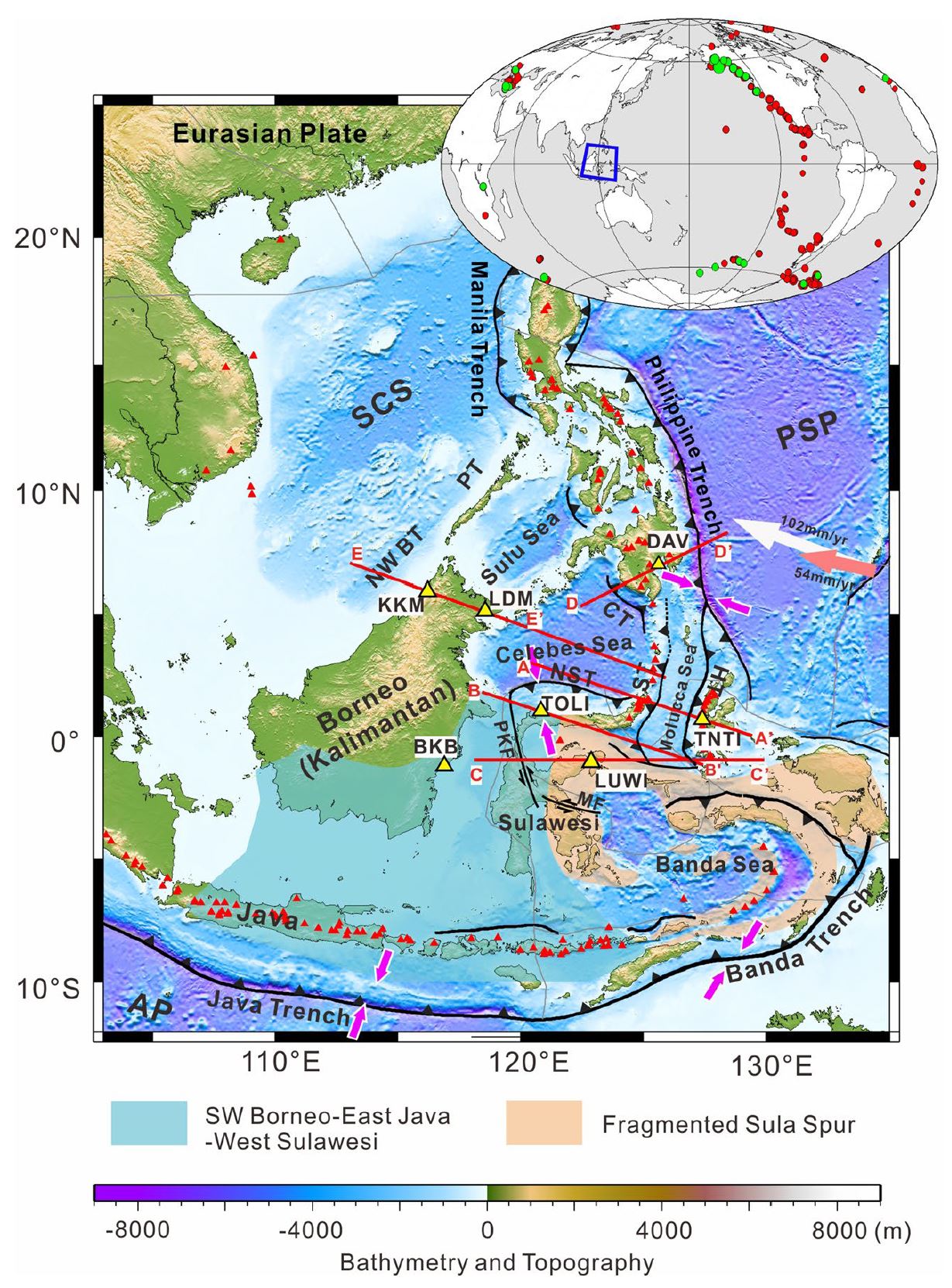
Bathymetric and topographic map showing the locations of the seven broadband seismic stations used in this study and the tectonics of the study area. Yellow triangles mark the seismic stations. Solid red triangles
denote Quaternary volcanoes. The black sawtooth lines show the trench location. Translucent shaded regions indicate the ranges of two areas whose crust probably originated from Australian continental fragments and extension by rollback of the Banda slab (modified from R. Hall & Sevastjanova, 2012). Arrows indicate plate motion directions from two different absolute plate motion models (hotspot model (white): Gripp & Gordon, 2002; no-net-rotation model (pink): DeMets et al., 1994). Pink arrow pairs indicate convergence directions between plates or micro-plates on both sides of the trenches (Argus et al., 2011; Bird, 2003; Lallemand et al., 1998; C. Liu & Shi, 2021). Red lines denote the locations of velocity perturbation cross sections, which are further discussed in Figure 7. The scale for the bathymetry and topography is shown at the bottom. AP, Australian Plate; CT, Cotabato Trench; HT, Halmahera Trench; MF, Matano Fault; NST, North Sulawesi Trench; NW BT, Northwest Borneo Trough; PKF, Palu Koro Fault; PSP, Philippine Sea Plate; PT, Palawan Trough; SCS, South China Sea; ST, Sangihe Trench. In the inset, red circles show Mw > 6.0 teleseismic events with epicentral distances ranging from 85° to 135° occurring between 2009 and 2019. Green circles show the locations of 26 teleseismic events used in the final analysis. The blue quadrilateral shows the location of the study area.
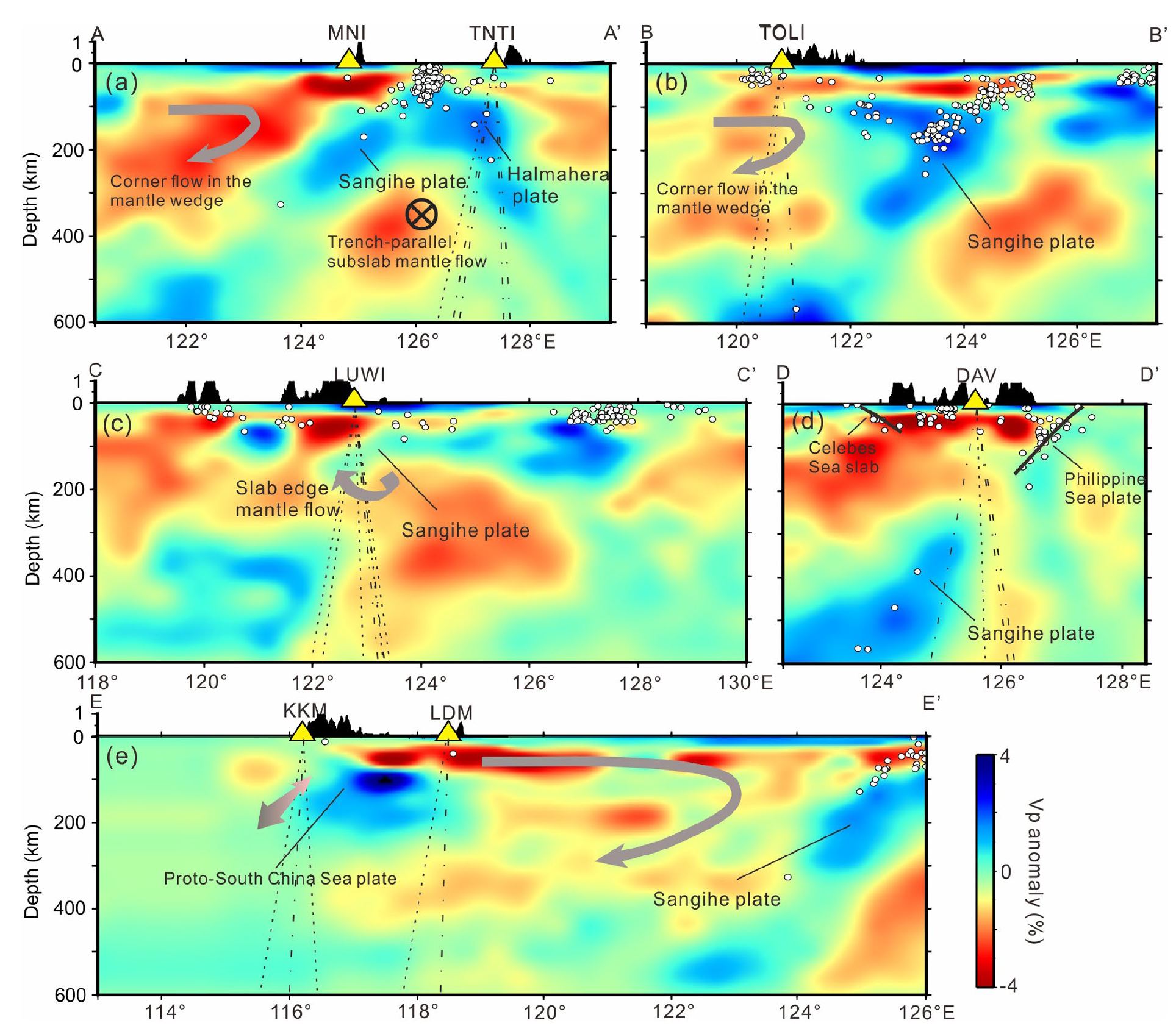
Interpretations of mantle flow patterns with the aid of Vp velocity perturbations in tomographic models by Amaru (2007). Mantle flow patterns along five vertical profiles (as shown in Figure 1) are presented. In general, the red and blue colors denote low and high Vp perturbations, respectively, whose scale is shown at the top right. White dots show earthquakes that occurred within a 20-km width along each profile. Yellow triangles represent stations used in this study shown in Figure 1 and station MNI from Di Leo et al. (2012b) shown in Figure 6. White dots show local seismicity spanning from 1990 to 2020 with magnitude >5 (the catalog is from USGS). Dotted lines delineate raypaths of SKS phases in the upper mantle defined by the source-receiver pairs. Topography is also depicted above each profile by the black areas. The gray bent arrows, and the circles with a cross and with a dot indicate the interpreted mantle flow
patterns.
Cartoon illustrating various types of mantle flow (red arrows) above, below, and around the down-going Molucca Sea plate, which are interpreted according to the results from this study and Di Leo et al. (2012a). At the stations, the orientation of each solid thick bar indicates the average fast polarization direction at the station, and the bar length is proportional to the average delay time. The SKS-wave raypaths in the upper mantle are delineated with curved black lines.

(a) Sketch of the Molucca Sea subduction zone and its vicinity. (b) Cross section (A-B) demonstrating the structure of arc-arc collision zone (modified after Hall and Smyth [2008]). (c) Distribution of earthquake events (2011.1.1–2015.12.31) and focal mechanism; the insert shows the vertical profile of epicenters sliced at position B-B0 . The black
dashed line in Figure 1a is the position of cross section A-B in Figure 1b, and the red solid lines in Figure 1c are the cross sections of the seismic tomographic velocity model in Figure 2.

Vertical slices of seismic velocity beneath the Molucca Sea and its surrounding regions, in which positive velocity anomalies outline the unique shape of the subducting Molucca Sea plate. The tomographic images are sliced from the global P wave velocity anomaly model UU-P07 [Amaru, 2007] along positions shown in Figure 1c.

Cartoon of end-member models illustrating effects of the order of subduction initiation, the mobility and thickness of the overriding plates on slab morphology, and migration of the overriding plates during DDS. Idealized DDS features (a) symmetrical subduction of slabs and (b–d) asymmetrical plate shape resulted from influence of order of subduction initiation, mobility, and thickness of overriding plates, respectively. (e) Tentative interpretation of formation of the asymmetrical DDS observed in the Molucca Sea region. Size of arrows indicate relative scale of the subduction-induced mantle flow.
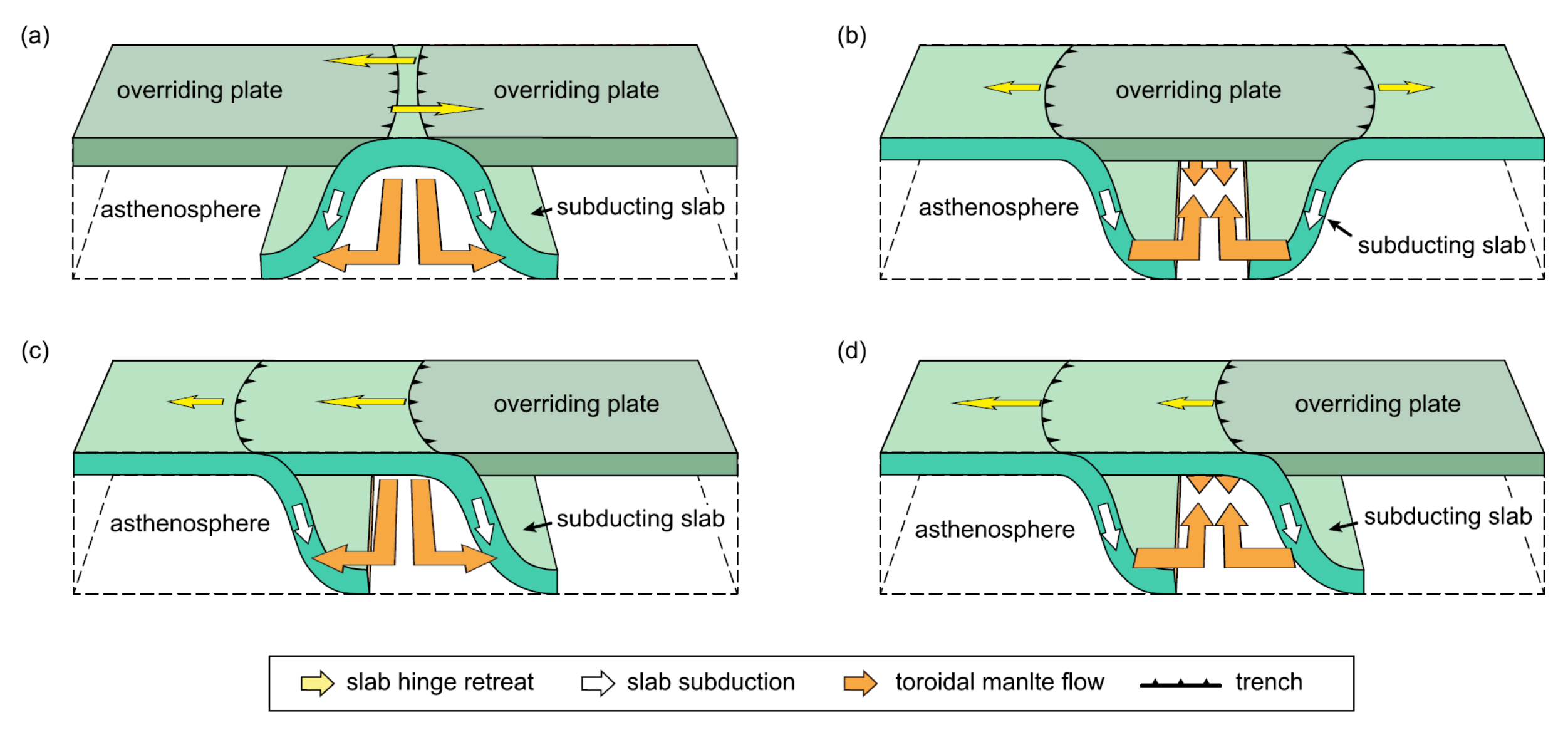
Cartoons illustrating several forms of double subduction. (a) Divergent double subduction (descripted in this study and by Soesoo et al. [1997], Di Leo et al. [2014], Li et al., [2014], etc.). (b) Double subduction with opposite dipping directions (descripted by Maruyama et al. [ 2007]). (c and d) Convergent double subduction (descripted by Jagoutz et al. [2015] and Billen [2015]). In all of these case, sustainable subduction of the oceanic plate(s) requires smooth escape (Figures 17a and 17c) of the slab-trapped mantle or replenishment of external materials of mantle into the void space left by slab rollback (Figures 17b and 17d). The toroidal mantle flow (orange arrows) plays a dominant role in
redistribution of material during all these types of double subduction.

Slab constraints for the SW Philippine Sea and surrounding areas. (a) Philippine Trench slab, Molucca Sea slabs, and detached “deep Ayu Trough” midslab maps. (b) Three-dimensional oblique view from west showing projected seismicity within 50 km of the Philippine Trench and Molucca Sea west midslab surfaces. (c) Unfolded Philippine Trench and Molucca Sea slabs colored by their dVp midslab seismic velocities. (d and e) MITP08 vertical tomographic cross sections and Benioff zone seismicity (red spheres) showing the interpreted fast-slab anomalies. Section locations are shown in Figure 21a. Note that the unfolded Molucca Sea slab in Figure 21c was the minimumlength model. A longer unfolded Molucca Sea slab is possible based on possible deeper (>900 km) anomalies in Figure 21b and the slab buckling in Figure 21e. PSP, Philippine Sea plate; Phil, Philippines; MS, Molucca Sea.
Tectonic Background: 02 AUGUST 2024 M 6.8 reverse faulting earthquake
- Here is a map that shows a simplified version of the subduction zones in the region (Galgana et al., 2007).
- Here is a map that shows the tectonic faults in central Philippines. The northern tip of Mindanao is in the lower right part of the map (Rimando et al., 2020).
- This is a low angle oblique view of the tectonic plates from Rimando et al., (2020).
- The location of cross section X-X’ is shown on the map above.

Physical map of the Philippines, showing topography and bathymetry. The two opposing subduction zones (the Manila Trench and the Philippine Trench/East Luzon Trough), major plates (SUND and PHSP) and the major Philippine Fault System with splays in Luzon (yellow lines) are mapped (basemap derived from the UNAVCO Jules Verne Navigator).
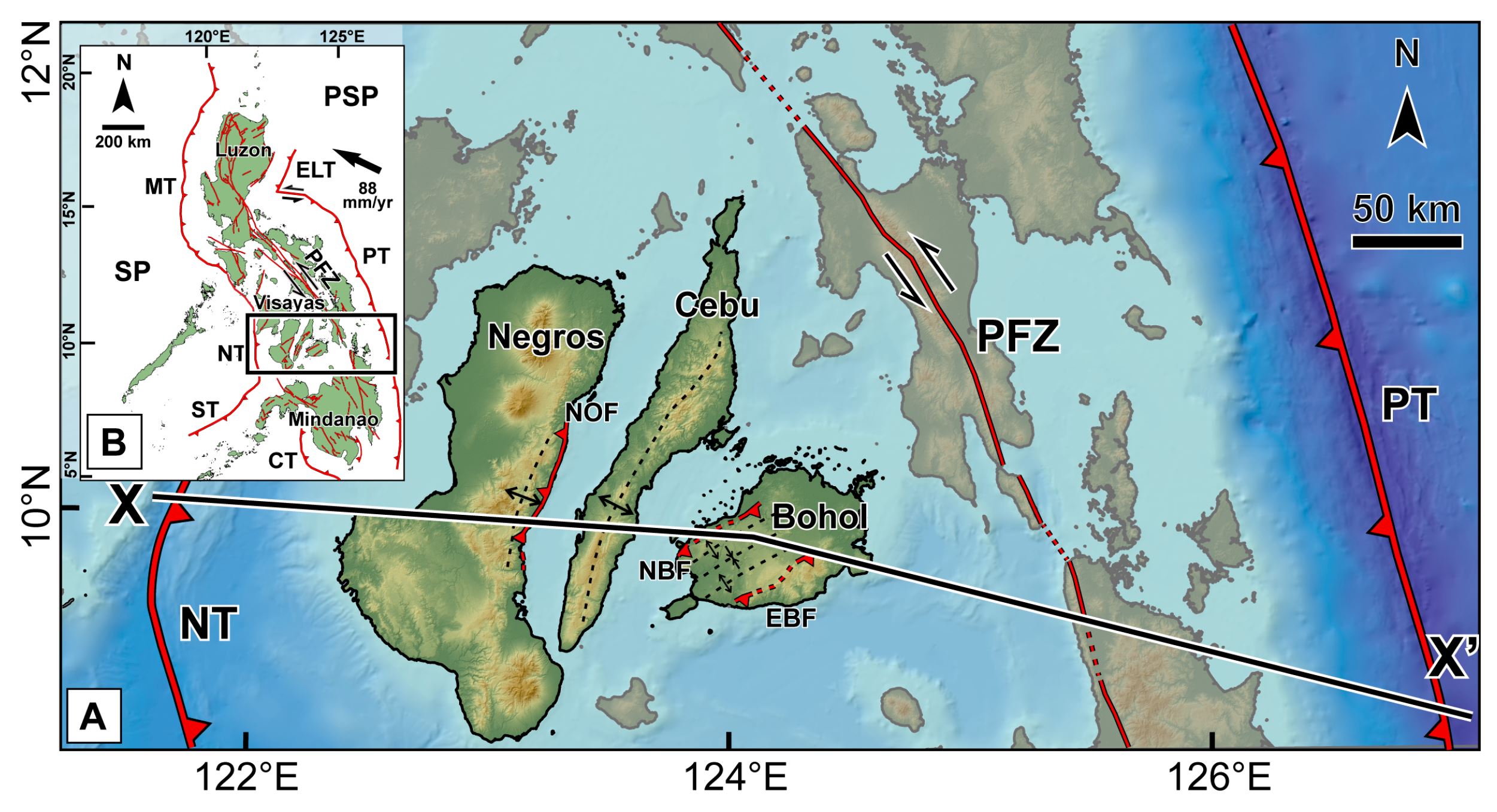
Currently known, Quaternary-active shortening structures in west-central Philippines. (A). Map highlighting the known late Quaternary-active folds and faults on the islands of Bohol, Cebu, and Negros. X—X′ indicates the location of the sectional-view schematic block diagram in Figure 8. NT—Negros Trench, PT—Philippine Trench, and PFZ—Philippine Fault Zone. (B). Inset map showing the location (black rectangle) of Figure 7A in the Philippine archipelago and its tectonic context.
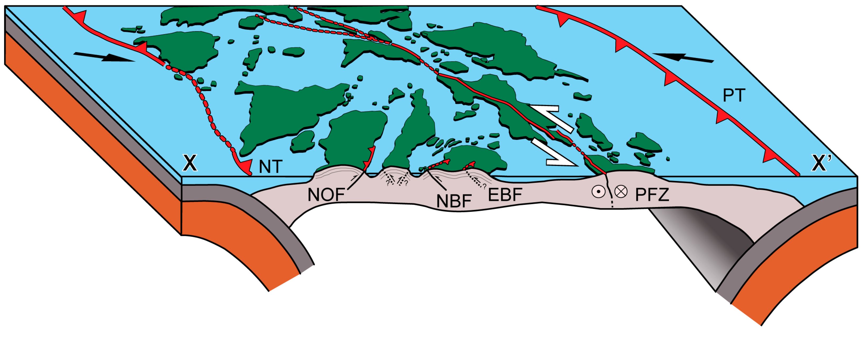
Schematic block diagram showing the structural and kinematic relationships of the Philippine Trench (PT), Negros Trench (NT), Philippine Fault Zone (PFZ), and some of the active shortening structures (i.e., faults and folds) in central Philippines (Bohol, Cebu, and Negros islands) along transect X—X′ in Figure 9. NOF—Negros Oriental Fault; NBF—North Bohol Fault; EBF—East Bohol Fault.
Shaking Intensity
- Here is a figure that shows a more detailed comparison between the modeled intensity and the reported intensity. Both data use the same color scale, the Modified Mercalli Intensity Scale (MMI). More about this can be found here. The colors and contours on the map are results from the USGS modeled intensity. The DYFI data are plotted as colored dots (color = MMI, diameter = number of reports).
- In the upper panel is the USGS Did You Feel It reports map, showing reports as colored dots using the MMI color scale. Underlain on this map are colored areas showing the USGS modeled estimate for shaking intensity (MMI scale).
- In the lower panel is a plot showing MMI intensity (vertical axis) relative to distance from the earthquake (horizontal axis). The models are represented by the green and orange lines. The DYFI data are plotted as light blue dots. The mean and median (different types of “average”) are plotted as orange and purple dots. Note how well the reports fit the green line (the model that represents how MMI works based on quakes in California).
- Below the map and the lower plot is the USGS MMI Intensity scale, which lists the level of damage for each level of intensity, along with approximate measures of how strongly the ground shakes at these intensities, showing levels in acceleration (Peak Ground Acceleration, PGA) and velocity (Peak Ground Velocity, PGV).
Seismic Hazard and Seismic Risk
- These are the two maps shown in the map above, the GEM Seismic Hazard and the GEM Seismic Risk maps from Pagani et al. (2018) and Silva et al. (2018).
- The GEM Seismic Hazard Map:
- The Global Earthquake Model (GEM) Global Seismic Hazard Map (version 2018.1) depicts the geographic distribution of the Peak Ground Acceleration (PGA) with a 10% probability of being exceeded in 50 years, computed for reference rock conditions (shear wave velocity, VS30, of 760-800 m/s). The map was created by collating maps computed using national and regional probabilistic seismic hazard models developed by various institutions and projects, and by GEM Foundation scientists. The OpenQuake engine, an open-source seismic hazard and risk calculation software developed principally by the GEM Foundation, was used to calculate the hazard values. A smoothing methodology was applied to homogenise hazard values along the model borders. The map is based on a database of hazard models described using the OpenQuake engine data format (NRML). Due to possible model limitations, regions portrayed with low hazard may still experience potentially damaging earthquakes.
- Here is a view of the GEM seismic hazard map for Indonesia and the Philippines.
- The GEM Seismic Risk Map:
- The Global Seismic Risk Map (v2018.1) presents the geographic distribution of average annual loss (USD) normalised by the average construction costs of the respective country (USD/m2) due to ground shaking in the residential, commercial and industrial building stock, considering contents, structural and non-structural components. The normalised metric allows a direct comparison of the risk between countries with widely different construction costs. It does not consider the effects of tsunamis, liquefaction, landslides, and fires following earthquakes. The loss estimates are from direct physical damage to buildings due to shaking, and thus damage to infrastructure or indirect losses due to business interruption are not included. The average annual losses are presented on a hexagonal grid, with a spacing of 0.30 x 0.34 decimal degrees (approximately 1,000 km2 at the equator). The average annual losses were computed using the event-based calculator of the OpenQuake engine, an open-source software for seismic hazard and risk analysis developed by the GEM Foundation. The seismic hazard, exposure and vulnerability models employed in these calculations were provided by national institutions, or developed within the scope of regional programs or bilateral collaborations.
- Here is a view of the GEM seismic risk map for Indonesia and the Philippines.


Potential for Ground Failure
- Below are a series of maps that show the potential for landslides and liquefaction. These are all USGS data products.
There are many different ways in which a landslide can be triggered. The first order relations behind slope failure (landslides) is that the “resisting” forces that are preventing slope failure (e.g. the strength of the bedrock or soil) are overcome by the “driving” forces that are pushing this land downwards (e.g. gravity). The ratio of resisting forces to driving forces is called the Factor of Safety (FOS). We can write this ratio like this:FOS = Resisting Force / Driving Force
- When FOS > 1, the slope is stable and when FOS < 1, the slope fails and we get a landslide. The illustration below shows these relations. Note how the slope angle α can take part in this ratio (the steeper the slope, the greater impact of the mass of the slope can contribute to driving forces). The real world is more complicated than the simplified illustration below.
- Landslide ground shaking can change the Factor of Safety in several ways that might increase the driving force or decrease the resisting force. Keefer (1984) studied a global data set of earthquake triggered landslides and found that larger earthquakes trigger larger and more numerous landslides across a larger area than do smaller earthquakes. Earthquakes can cause landslides because the seismic waves can cause the driving force to increase (the earthquake motions can “push” the land downwards), leading to a landslide. In addition, ground shaking can change the strength of these earth materials (a form of resisting force) with a process called liquefaction.
- Sediment or soil strength is based upon the ability for sediment particles to push against each other without moving. This is a combination of friction and the forces exerted between these particles. This is loosely what we call the “angle of internal friction.” Liquefaction is a process by which pore pressure increases cause water to push out against the sediment particles so that they are no longer touching.
- An analogy that some may be familiar with relates to a visit to the beach. When one is walking on the wet sand near the shoreline, the sand may hold the weight of our body generally pretty well. However, if we stop and vibrate our feet back and forth, this causes pore pressure to increase and we sink into the sand as the sand liquefies. Or, at least our feet sink into the sand.
- Below is a diagram showing how an increase in pore pressure can push against the sediment particles so that they are not touching any more. This allows the particles to move around and this is why our feet sink in the sand in the analogy above. This is also what changes the strength of earth materials such that a landslide can be triggered.
- Below is a diagram based upon a publication designed to educate the public about landslides and the processes that trigger them (USGS, 2004). Additional background information about landslide types can be found in Highland et al. (2008). There was a variety of landslide types that can be observed surrounding the earthquake region. So, this illustration can help people when they observing the landscape response to the earthquake whether they are using aerial imagery, photos in newspaper or website articles, or videos on social media. Will you be able to locate a landslide scarp or the toe of a landslide? This figure shows a rotational landslide, one where the land rotates along a curvilinear failure surface.
- Below is the liquefaction susceptibility and landslide probability map (Jessee et al., 2017; Zhu et al., 2017). Please head over to that report for more information about the USGS Ground Failure products (landslides and liquefaction). Basically, earthquakes shake the ground and this ground shaking can cause landslides.
- I use the same color scheme that the USGS uses on their website. Note how the areas that are more likely to have experienced earthquake induced liquefaction are in the valleys. Learn more about how the USGS prepares these model results here.


Social Media
#EarthquakeReport for M6.8 #Gempa #Earthquake in the #Philippines
mechanism & depth suggest to be on megathrust subduction zone (?)
possible local #Tsunami (?)https://t.co/1vVYkhSe03in region of M 7.6 in December '23: https://t.co/CVr22I6vTa pic.twitter.com/kQOgMaOwOl
— Jason "Jay" R. Patton (@patton_cascadia) August 2, 2024
- 2024.08.02 M 6.8 Philippines
- 2024.07.11 M 7.1 Philippines
- 2023.12.02 M 7.6 Philippines
- 2022.07.27 M 7.0 Philippines (poster)
- 2021.08.11 M 7.1 Philippines (poster)
- 2019.11.14 M 7.1 Halmahera
- 2019.07.14 M 7.3 Halmahera
- 2018.12.29 M 7.0 Philippines
- 2017.12.08 M 6.5 Caroline Ridge
- 2017.12.09 M 6.5 Caroline Ridge Update #1
- 2017.08.11 M 6.2 Philippines
- 2017.04.28 M 6.9 Philippines
- 2017.04.08 M 5.9 Philippines
- 2017.01.10 M 7.3 Celebes Sea
- 2016.07.29 M 7.7 Mariana
- 2015.03.17 M 6.2 Molucca Sea
- 2014.11.26 M 6.8 Molucca Sea
- 2014.11.21 M 6.5 Molucca Sea
- 2014.11.15 M 7.1 Molucca Sea
Philippines | Western Pacific
Earthquake Reports
- Frisch, W., Meschede, M., Blakey, R., 2011. Plate Tectonics, Springer-Verlag, London, 213 pp.
- Hayes, G., 2018, Slab2 – A Comprehensive Subduction Zone Geometry Model: U.S. Geological Survey data release, https://doi.org/10.5066/F7PV6JNV.
- Holt, W. E., C. Kreemer, A. J. Haines, L. Estey, C. Meertens, G. Blewitt, and D. Lavallee (2005), Project helps constrain continental dynamics and seismic hazards, Eos Trans. AGU, 86(41), 383–387, , https://doi.org/10.1029/2005EO410002. /li>
- Jessee, M.A.N., Hamburger, M. W., Allstadt, K., Wald, D. J., Robeson, S. M., Tanyas, H., et al. (2018). A global empirical model for near-real-time assessment of seismically induced landslides. Journal of Geophysical Research: Earth Surface, 123, 1835–1859. https://doi.org/10.1029/2017JF004494
- Kreemer, C., J. Haines, W. Holt, G. Blewitt, and D. Lavallee (2000), On the determination of a global strain rate model, Geophys. J. Int., 52(10), 765–770.
- Kreemer, C., W. E. Holt, and A. J. Haines (2003), An integrated global model of present-day plate motions and plate boundary deformation, Geophys. J. Int., 154(1), 8–34, , https://doi.org/10.1046/j.1365-246X.2003.01917.x.
- Kreemer, C., G. Blewitt, E.C. Klein, 2014. A geodetic plate motion and Global Strain Rate Model in Geochemistry, Geophysics, Geosystems, v. 15, p. 3849-3889, https://doi.org/10.1002/2014GC005407.
- Meyer, B., Saltus, R., Chulliat, a., 2017. EMAG2: Earth Magnetic Anomaly Grid (2-arc-minute resolution) Version 3. National Centers for Environmental Information, NOAA. Model. https://doi.org/10.7289/V5H70CVX
- Müller, R.D., Sdrolias, M., Gaina, C. and Roest, W.R., 2008, Age spreading rates and spreading asymmetry of the world’s ocean crust in Geochemistry, Geophysics, Geosystems, 9, Q04006, https://doi.org/10.1029/2007GC001743
- Pagani,M. , J. Garcia-Pelaez, R. Gee, K. Johnson, V. Poggi, R. Styron, G. Weatherill, M. Simionato, D. Viganò, L. Danciu, D. Monelli (2018). Global Earthquake Model (GEM) Seismic Hazard Map (version 2018.1 – December 2018), DOI: 10.13117/GEM-GLOBAL-SEISMIC-HAZARD-MAP-2018.1
- Silva, V ., D Amo-Oduro, A Calderon, J Dabbeek, V Despotaki, L Martins, A Rao, M Simionato, D Viganò, C Yepes, A Acevedo, N Horspool, H Crowley, K Jaiswal, M Journeay, M Pittore, 2018. Global Earthquake Model (GEM) Seismic Risk Map (version 2018.1). https://doi.org/10.13117/GEM-GLOBAL-SEISMIC-RISK-MAP-2018.1
- Zhu, J., Baise, L. G., Thompson, E. M., 2017, An Updated Geospatial Liquefaction Model for Global Application, Bulletin of the Seismological Society of America, 107, p 1365-1385, https://doi.org/0.1785/0120160198
- Aurelio, M.A., Peña, R.E., Taguibao, K.J.L., Sculpting the Philippine archipelago since the Cretaceous through rifting, oceanic spreading, subduction, obduction, collision and strike-slip faulting: contribution to IGMA5000, Journal of Asian Earth Sciences (2012), doi: http://dx.doi.org/10.1016/j.jseaes.2012.10.007
- Aurelio, M., Lagmay, M., Escudero, J. A., and Catugas, S., 2021, Another large earthquake strikes the southern Philippines, Temblor, http://doi.org/10.32858/temblor.196
- Bock et al., 2003. Crustal motion in Indonesia from Global Positioning System measurements in JGR, v./ 108, no. B8, 2367, doi:10.1029/2001JB000324
- Cao, L., He, X., Zhao, L., Lü, C., Hao, T., Zhao, M., & Qiu, X. (2021). Mantle flow patterns beneath the junction of multiple subduction systems between the Pacific and Tethys domains, SE Asia: Constraints from SKS-wave splitting measurements. Geochemistry, Geophysics, Geosystems, 22, e2021GC009700. https://doi.org/10.1029/2021GC009700
- Hall, R., 2011. Australia–SE Asia collision: plate tectonics and crustal flow in Hall, R., Cottam, M. A. &Wilson, M. E. J. (eds) The SE Asian Gateway: History and Tectonics of the Australia–Asia Collision. Geological Society, London, Special Publications, 355, 75–109.
- Fan, J-k., Wu, S-g., Spence, G., 2015. Tomographic evidence for a slab tear induced by fossil ridge subduction at Manila Trench, South China Sea in International Geology Review, v. 57, p. 998-1013, DOI: 10.1080/00206814.2014.929054
- Hayes, G.P., Wald, D.J., and Johnson, R.L., 2012. Slab1.0: A three-dimensional model of global subduction zone geometries in, J. Geophys. Res., 117, B01302, doi:10.1029/2011JB008524
- Hsu, Y-J., Yu, S-B., Song, T-R.A., and Bacolcol, T., 2012. Plate coupling along the Manila subduction zone between Taiwan and northern Luzo in Journal of Asian Earth Sciences, v. 51, p. 98-108
- McCaffrey, R., Silver, E.A., and Raitt, R.W., 1980. Crustal Structure of the Molucca Sea Collision Zone, Indonesia in The Tectonic and Geologic Evolution of Southeast Asian Seas and Islands-Geophysical Monograph 23, p. 161-177.
- Noda, A., 2013. Strike-Slip Basin – Its Configuration and Sedimentary Facies in Mechanism of Sedimentary Basin Formation – Multidisciplinary Approach on Active Plate Margins http://www.intechopen.com/books/mechanism-of-sedimentarybasin-formation-multidisciplinary-approach-on-active-plate-margins http://dx.doi.org/10.5772/56593
- Rimando RE, Rimando JM, Lim RB. Complex Shear Partitioning Involving the 6 February 2012 MW 6.7 Negros Earthquake Ground Rupture in Central Philippines. Geosciences. 2020; 10(11):460. https://doi.org/10.3390/geosciences10110460
- Smoczyk, G.M., Hayes, G.P., Hamburger, M.W., Benz, H.M., Villaseñor, Antonio, and Furlong, K.P., 2013. Seismicity of the Earth 1900–2012 Philippine Sea plate and vicinity: U.S. Geological Survey Open-File Report 2010–1083-M, 1 sheet, scale 1:10,000,000.
- Waltham et al., 2008. Basin formation by volcanic arc loading in GSA Special Papers 2008, v. 436, p. 11-26.
- Wang, K., and Bilek, S.L., 2014. Invited review paper: Fault creep caused by subduction of rough seafloor relief in Tectonophysics, v. 610, p./ 1-24.
- Wu, J., J. Suppe, R. Lu, and R. Kanda, 2016. Philippine Sea and East Asian plate tectonics since 52 Ma constrained by new subducted slab reconstruction methods, J. Geophys. Res. Solid Earth, 121, doi:10.1002/2016JB012923.
- Zahirovic et al., 2014. The Cretaceous and Cenozoic tectonic evolution of Southeast Asia in Solid Earth, v. 5, p. 227-273, doi:10.5194/se-5-227-2014.
References:
Basic & General References
Specific References
Return to the Earthquake Reports page.
- Sorted by Magnitude
- Sorted by Year
- Sorted by Day of the Year
- Sorted By Region