I am slowly catching up with the Earthquake Reports! I have been ill on and off and I had lots of field work this summer conducting a paleoseismic investigation for a thrust fault I discovered in 2018.
On 28 July 2026 there was a magnitude M 6.8 earthquake in southern Japan near the city of Kumamoto.
https://earthquake.usgs.gov/earthquakes/eventpage/us6000tgb9/executive
This earthquake is in the same area as an earthquake sequence from 2016. Below I present some information about the 2016 earthquake that has been published since that earthquake.
Both the 2016 and this 2026 earthquakes have right-lateral strike-slip earthquake mechanisms.
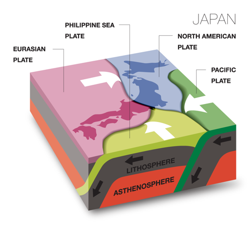
Japan sits atop a suite of convergent plate boundaries, subduction zones, where several different plates are subducting beneath several other plates.
Here is an excellent diagram first published by Dr. Austin Elliot on the AGU blog Trembling Earth. We can see the configuration of the plates in this complicated region.
However, these two earthquake sequences were along crustal faults in the upper plate, not along the subduction zone.
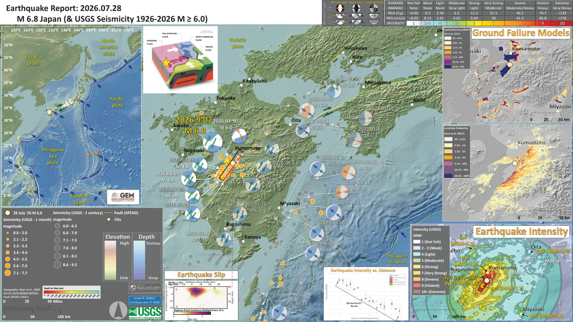
Below is my interpretive poster for this earthquake
- I plot the seismicity from the past month, with diameter representing magnitude (see legend). I include earthquake epicenters from 1926-2026 with magnitudes M ≥ 6.0 in one version.
- I plot the USGS fault plane solutions (moment tensors in blue and focal mechanisms in orange), possibly in addition to some relevant historic earthquakes.
- A review of the basic base map variations and data that I use for the interpretive posters can be found on the Earthquake Reports page. I have improved these posters over time and some of this background information applies to the older posters.
- Some basic fundamentals of earthquake geology and plate tectonics can be found on the Earthquake Plate Tectonic Fundamentals page.
- In the upper left is a map showing the plate tectonic boundaries (from the USGS).
- To the right of the tectonic overview map is a low angle oblique diagram showing the plate tectonic configuration (from the AGU Trembling Earth blog).
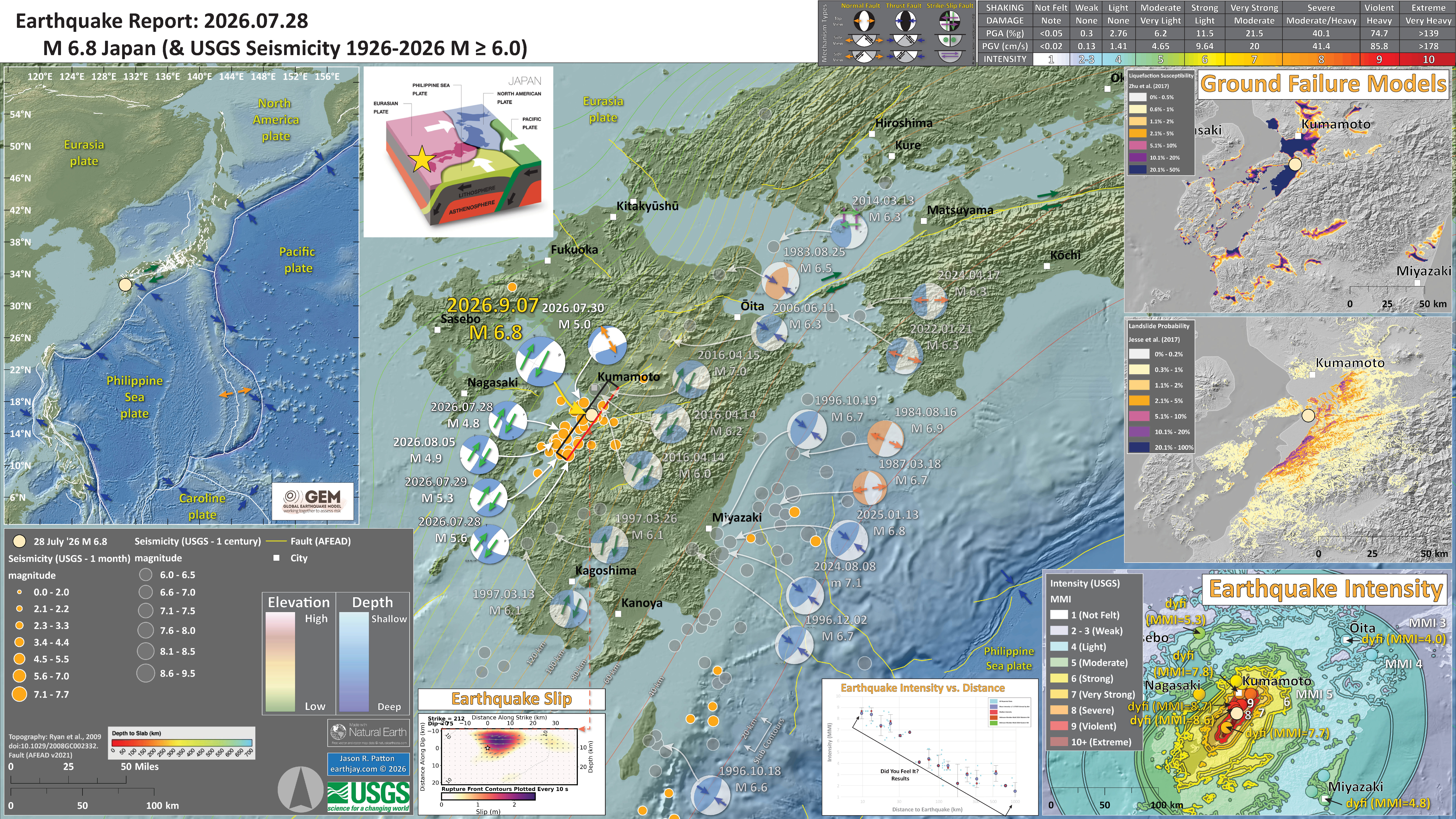
- In the lower right corner is a map that shows the M 6.8 earthquake intensity using the modified Mercalli intensity scale. Earthquake intensity is a measure of how strongly the Earth shakes during an earthquake, so gets smaller the further away one is from the earthquake epicenter. The map colors represent a model of what the intensity may be. The USGS has a system called “Did You Feel It?” (DYFI) where people enter their observations from the earthquake and the USGS calculates what the intensity was for that person. The dots with yellow labels show what people actually felt in those different locations.
- To the upper left of the intensity map is a plot that shows the same intensity (both modeled and reported) data as displayed on the map. Note how the intensity gets smaller with distance from the earthquake.
- In the upper right corner are two maps showing the possibility of earthquake triggered landslides and earthquake induced liquefaction for these two earthquakes.
- In the center left is the USGS finite fault model that shows their estimate of the amount that the fault slipped during this earthquake. I show the location of this fault model on the map outlined as a black rectangle with a red line showing the top of the fault, where it intersects the ground surface.
I include some inset figures. Some of the same figures are located in different places on the larger scale map below.
- Here is the map with a month’s seismicity plotted.
Other Report Pages
Shaking Intensity
- Here is a figure that shows a more detailed comparison between the modeled intensity and the reported intensity. Both data use the same color scale, the Modified Mercalli Intensity Scale (MMI). More about this can be found here. The colors and contours on the map are results from the USGS modeled intensity. The DYFI data are plotted as colored dots (color = MMI, diameter = number of reports).
- In the upper panel is the USGS Did You Feel It reports map, showing reports as colored dots using the MMI color scale. Underlain on this map are colored areas showing the USGS modeled estimate for shaking intensity (MMI scale).
- In the lower panel is a plot showing MMI intensity (vertical axis) relative to distance from the earthquake (horizontal axis). The models are represented by the green and orange lines. The DYFI data are plotted as light blue dots. The mean and median (different types of “average”) are plotted as orange and purple dots. Note how well the reports fit the green line (the model that represents how MMI works based on quakes in California).
- Below the map and the lower plot is the USGS MMI Intensity scale, which lists the level of damage for each level of intensity, along with approximate measures of how strongly the ground shakes at these intensities, showing levels in acceleration (Peak Ground Acceleration, PGA) and velocity (Peak Ground Velocity, PGV).
Potential for Ground Failure
- Below are a series of maps that show the potential for landslides and liquefaction. These are all USGS data products.
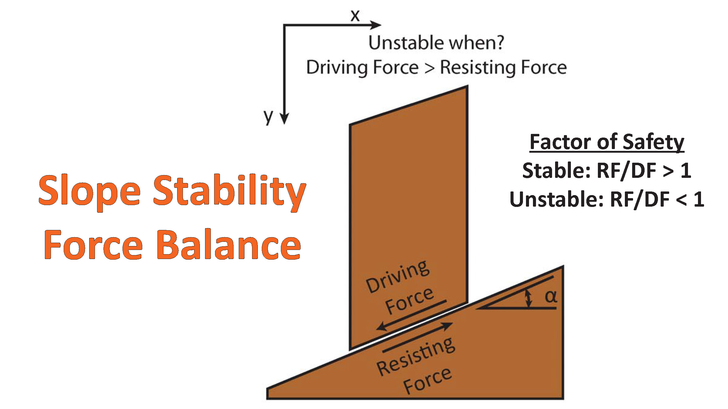
There are many different ways in which a landslide can be triggered. The first order relations behind slope failure (landslides) is that the “resisting” forces that are preventing slope failure (e.g. the strength of the bedrock or soil) are overcome by the “driving” forces that are pushing this land downwards (e.g. gravity). The ratio of resisting forces to driving forces is called the Factor of Safety (FOS). We can write this ratio like this:FOS = Resisting Force / Driving Force
- When FOS > 1, the slope is stable and when FOS < 1, the slope fails and we get a landslide. The illustration below shows these relations. Note how the slope angle α can take part in this ratio (the steeper the slope, the greater impact of the mass of the slope can contribute to driving forces). The real world is more complicated than the simplified illustration below.
- Landslide ground shaking can change the Factor of Safety in several ways that might increase the driving force or decrease the resisting force. Keefer (1984) studied a global data set of earthquake triggered landslides and found that larger earthquakes trigger larger and more numerous landslides across a larger area than do smaller earthquakes. Earthquakes can cause landslides because the seismic waves can cause the driving force to increase (the earthquake motions can “push” the land downwards), leading to a landslide. In addition, ground shaking can change the strength of these earth materials (a form of resisting force) with a process called liquefaction.
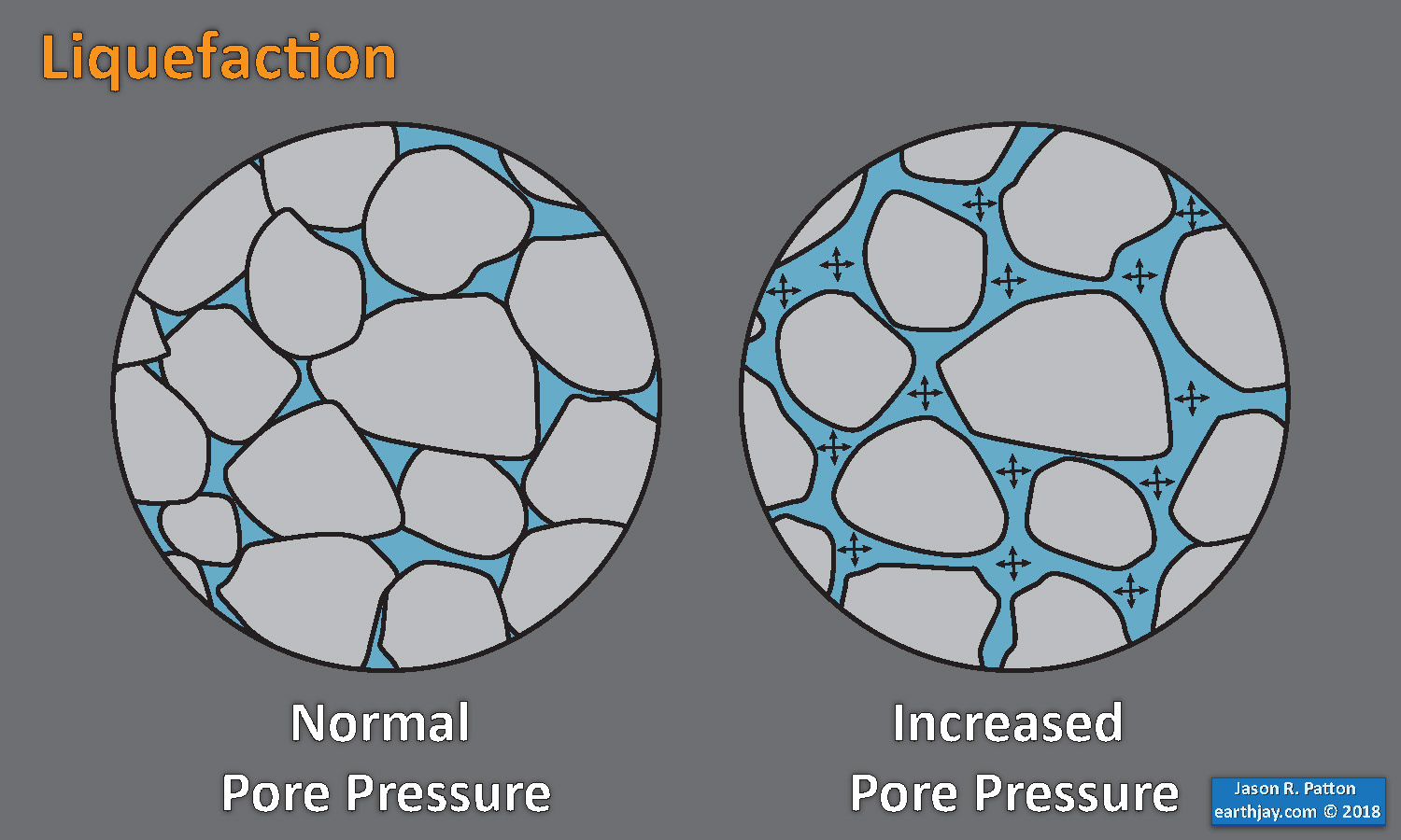
- Sediment or soil strength is based upon the ability for sediment particles to push against each other without moving. This is a combination of friction and the forces exerted between these particles. This is loosely what we call the “angle of internal friction.” Liquefaction is a process by which pore pressure increases cause water to push out against the sediment particles so that they are no longer touching.
- An analogy that some may be familiar with relates to a visit to the beach. When one is walking on the wet sand near the shoreline, the sand may hold the weight of our body generally pretty well. However, if we stop and vibrate our feet back and forth, this causes pore pressure to increase and we sink into the sand as the sand liquefies. Or, at least our feet sink into the sand.
- Below is a diagram showing how an increase in pore pressure can push against the sediment particles so that they are not touching any more. This allows the particles to move around and this is why our feet sink in the sand in the analogy above. This is also what changes the strength of earth materials such that a landslide can be triggered.
- Here Dr. Bohon demonstrates the phenomena of liquefaction.
- And, another video demonstration.
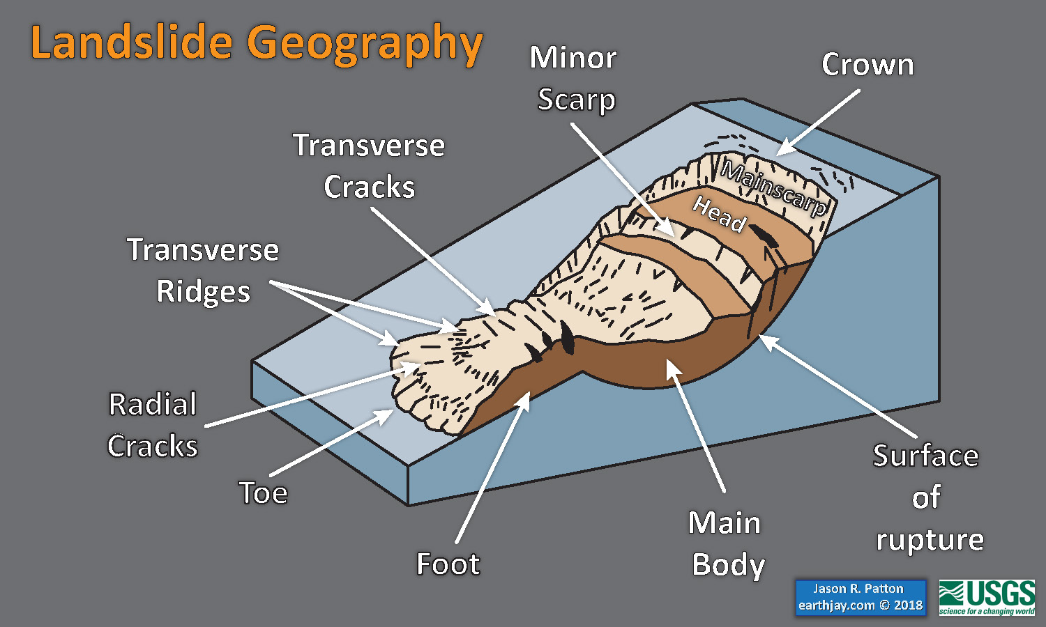
- Below is a diagram based upon a publication designed to educate the public about landslides and the processes that trigger them (USGS, 2004). Additional background information about landslide types can be found in Highland et al. (2008). There was a variety of landslide types that can be observed surrounding the earthquake region. So, this illustration can help people when they observing the landscape response to the earthquake whether they are using aerial imagery, photos in newspaper or website articles, or videos on social media. Will you be able to locate a landslide scarp or the toe of a landslide? This figure shows a rotational landslide, one where the land rotates along a curvilinear failure surface.
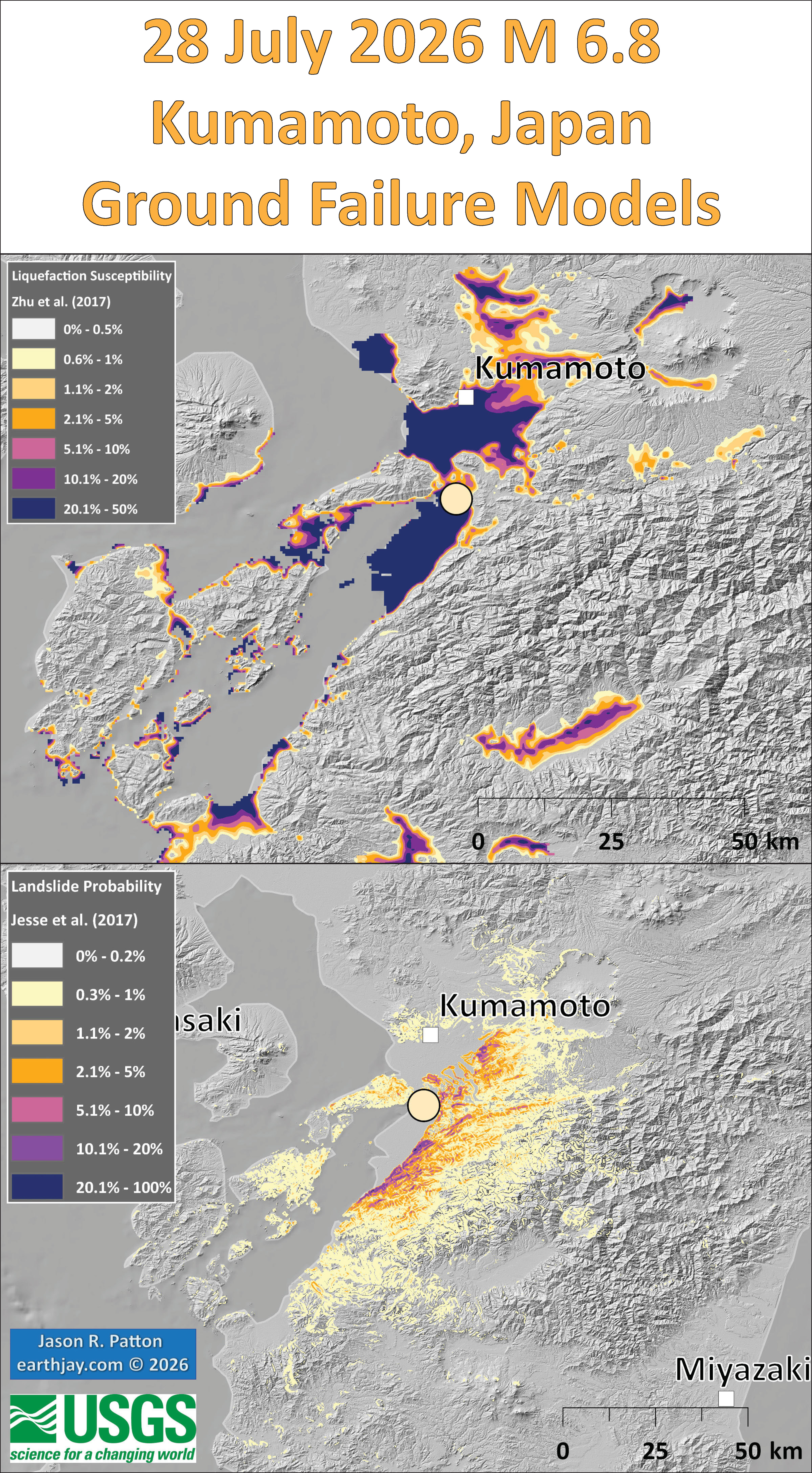
- Below is the liquefaction susceptibility and landslide probability map (Jessee et al., 2017; Zhu et al., 2017). Please head over to that report for more information about the USGS Ground Failure products (landslides and liquefaction). Basically, earthquakes shake the ground and this ground shaking can cause landslides.
- I use the same color scheme that the USGS uses on their website. Note how the areas that are more likely to have experienced earthquake induced liquefaction are in the valleys. Learn more about how the USGS prepares these model results here.
@drwendyrocksit #Liquefaction is a process by which water-saturated sediment temporarily loses strength and acts as a fluid. This can happen during #earthquake shaking. #geophysics #geology ♬ Quicksand – Hatchie
This liquefaction experiment conducted by the Tokyo Geological Survey of Japan at the Disaster Prevention Exhibition in 2015, shows the effects of different foundations and how hollow objects such as water pipes come to the surface [source, full video: https://t.co/xYLjPY4IHZ] pic.twitter.com/r8LXtmvrO0
— Massimo (@Rainmaker1973) April 17, 2021
Some Relevant Discussion and Figures
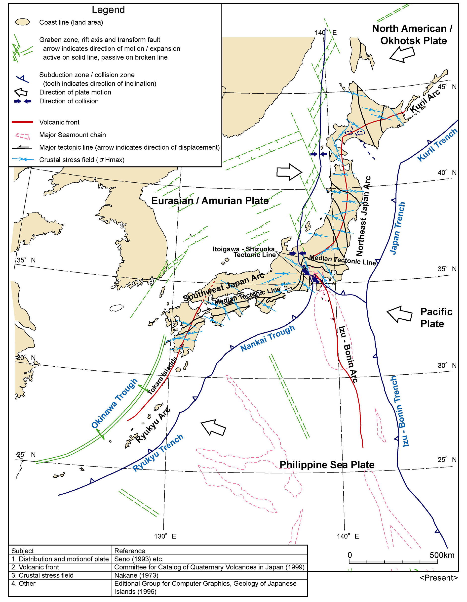
- This map shows the current tectonic configuration of this region, along with some inherited features from the tectonic past (e.g. green lines). This is from NUMO’s report: “Evaluating Site Suitability for a HLW Repository (Scientific Background and Practical Application of NUMO’s Siting Factors), NUMO-TR-04-04.”
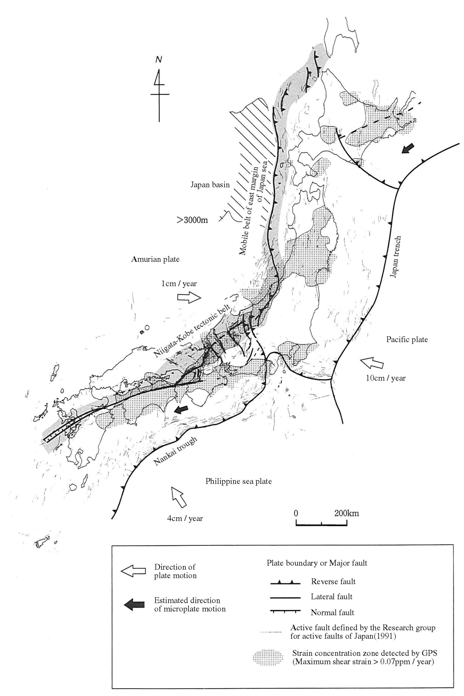
- Also from the NUMO report, this shows the Niigata-Kobe fold and thrust belt. In addition, this map shows a northwest striking convergent plate boundary along the southeastern boundary of Hokkaido. However, it cannot explain the interesting orientation of the M 6.2 deep (240 km) earthquake.
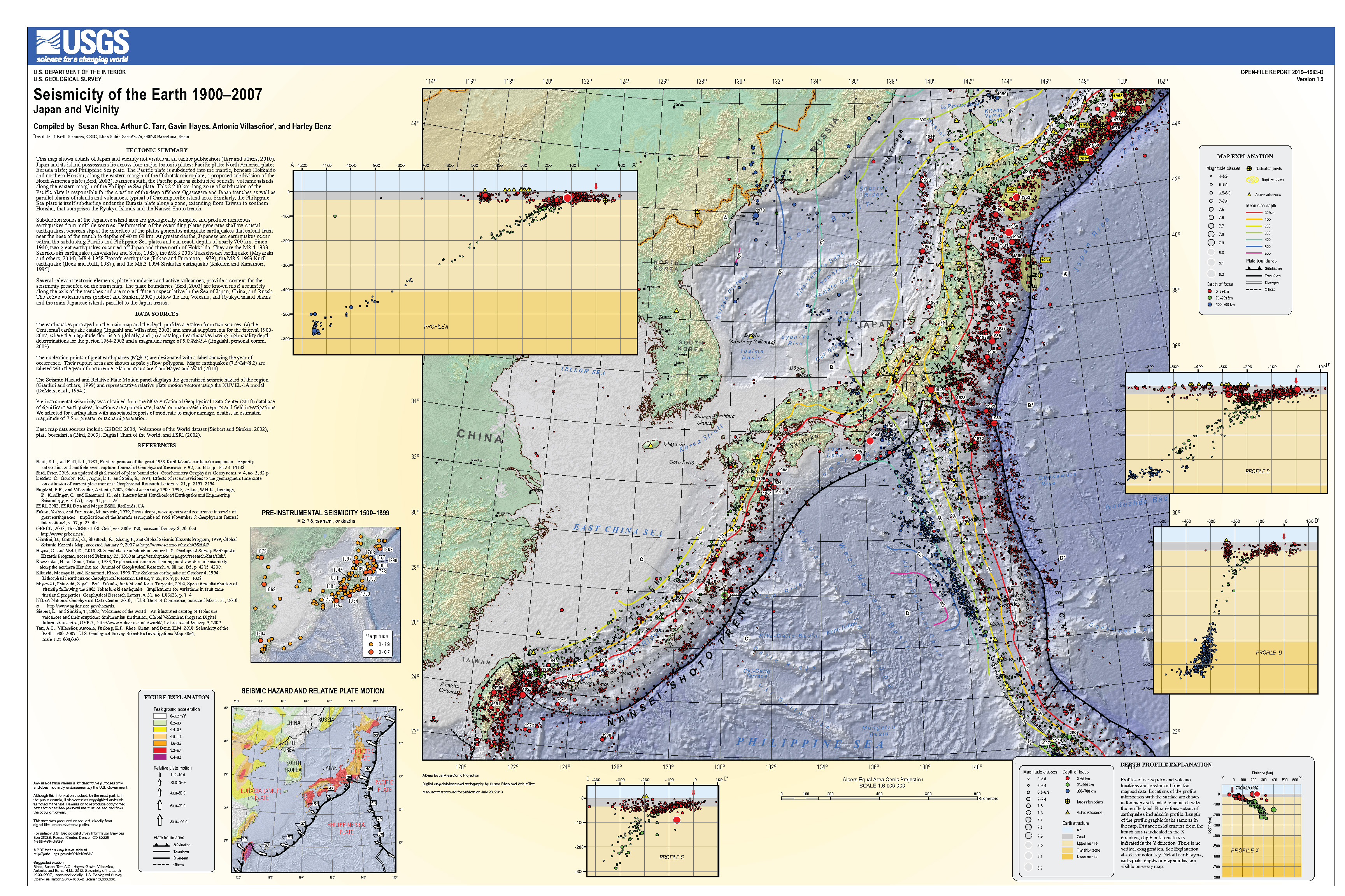
- Here is a USGS poster than summarizes the earthquake history and plate geometry for this region. This is the USGS Open File Report 2010-1083-D (Rhea et al., 2010).
- Here is the cool tectonic map from Liu et al. (2013). We all like cool maps! (right?)
- Here is a map from the recent update of the Japan National Seismic Hazard Maps, resulting from knowledge gained following the 2011 M 9.1 earthquake (Fujiwara et al., 2012). The color represents the chance that a region will experience ground shaking at or greater that Japan Meteorological Agency (JMA) seismic intensity 6 in the next 30 years. JMA intensity is a scale of shaking intensity similar to the Modified Mercalli Intensity (MMI) Scale. The numbers are different, so they are difficult to compare. The JMA intensity 6 is similar to MMI X. Today’s earthquakes are in a region of slightly elevated chance of ground shaking (between 6-26%). Today’s M 6.6 earthquake may have reached
- This is a fantastic educational video from IRIS that discusses the plate tectonics and mentions some earthquakes in the region of Japan.

Tectonic settings of the study region (black box). The solid sawtooth lines and the black dashed line denote the plate boundaries (Bird 2003). The red triangles denote the active volcanoes. The blue dashed lines and the pink lines denote the depth contours to the upper boundary of the subducting Pacific slab and that of the subducting Philippine Sea slab, respectively (Hasegawa et al. 2009; Zhao et al. 2012). The topography data are derived from the GEBCO_08 Grid, version 20100927, http://www.gebco.net. The ages of oceanic plates are from M¨uller et al. (2008).

2016 Earthquake
- Below we see some documentation of surface ruptures from the 2016 earthquake from Shirahama et al. (2016). This is part of a special publication full of papers devoted to this earthquake.
- Here is the map showing the spatial extent of their study. There are many other observations but these geological data are fundamentally the most important type of data that are used to validate or calibrate all other measurements and models.
- The field of paleoseismology is the study of prehistoric earthquakes. When we look at these direct observations from modern/historic earthquakes, think about what evidence may or may not make it into the geological record. In other words, what observations might be preserved to be seen in a few hundred or a few thousand years. Obviously, not all of these evidences will be preserved. So, when we look at the prehistoric evidence for earthquakes, we must recognize that our observations are a subset of the original evidence.
Here we will take a look at some of the observations from the 2016 earthquake sequence.
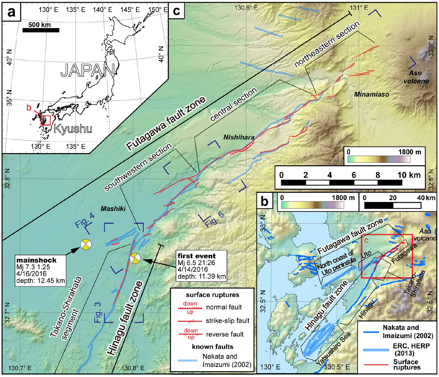
a Location of the study area in Kyushu, southwestern Japan. b Active faults in the western part of central Kyushu (blue lines after Nakata and Imaizumi 2002, light blue lines after ERC, HERP 2013) and the 2016 surface ruptures (red lines). c Distribution of surface ruptures associated with the 2016 Kumamoto earthquake sequence observed during our survey (red lines), previously mapped active faults (blue lines), and the best double couple solution of centroid moment tensor diagrams for the mainshock and the initial MJ 6.5 event (yellow beach balls) determined by the Japan Meteorological Agency, and unconfirmed ruptures interpreted from aerial photographs (Geospatial Information Authority of Japan 2016c) (dashed red lines)
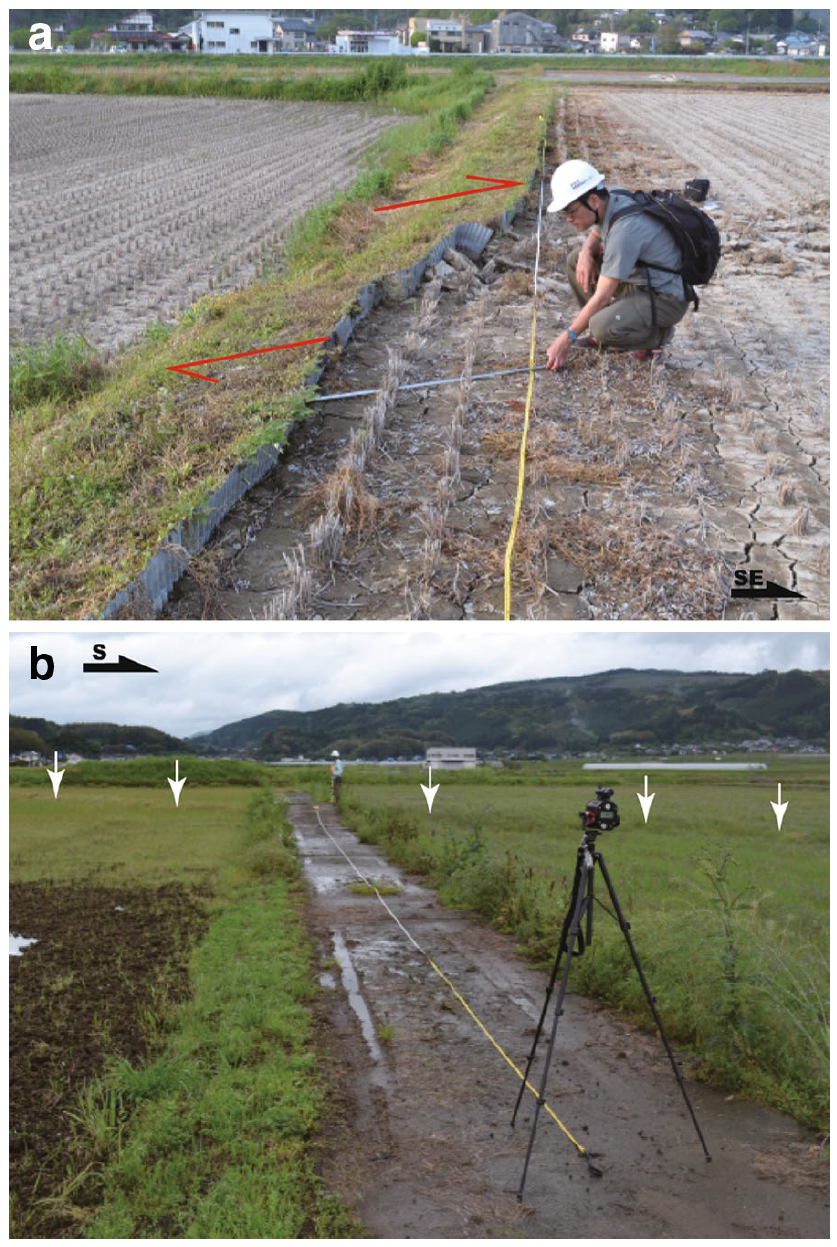
a Measuring horizontal displacement. The grassy footpath in the paddy field was displaced dextrally (red half-arrows). b Measuring a cross section. The east side of the road in the paddy field was uplifted relative to the west side along the surface rupture (white arrows). A handheld laser rangefinder was used to construct a cross section along the line of the yellow measuring tape
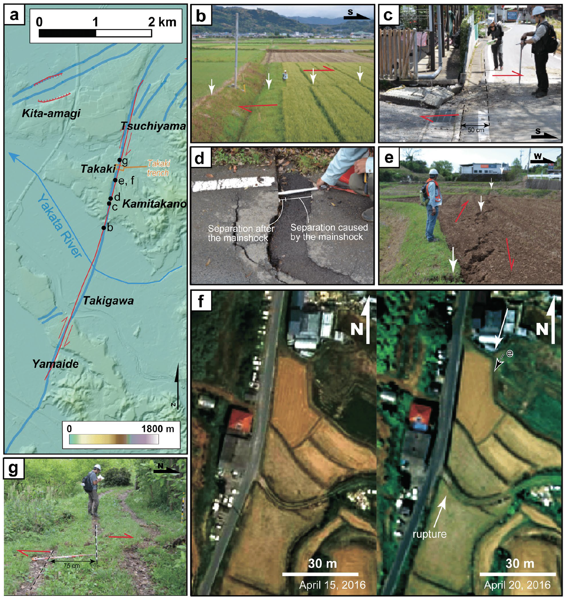
a Distribution of surface ruptures (red lines), previously mapped active fault traces (blue lines), and locations of photographs (solid circles) and the trench site (yellow box) along the Takano-Shirahata segment of the Hinagu fault zone (Fig. 1c). b Cultural features including rows of wheat displaced dextrally (red half-arrows) at Kamitakano along the rupture (white arrows). c Edge of a road displaced dextrally. d Postseismic activity shown by a crack in a paved road at Takaki. The open crack, filled with asphalt after the mainshock, opened further by the time the photograph was taken on April 28. e Array of left-stepping tension cracks produced by dextral faulting in the alluvial plain at Takaki, as seen on April 16 after the mainshock. f Aerial photographs of Takaki (Geospatial Information Authority of Japan 2016a, b) on April 15 (left) and April 20 (right). No surface rupture was apparent on April 15, whereas a distinct surface rupture displacing rice paddies and footpaths was discernible on April 20. The black arrow shows the location of E. g Dextral offset of wheel tracks by 75 cm on a farm road in Takaki
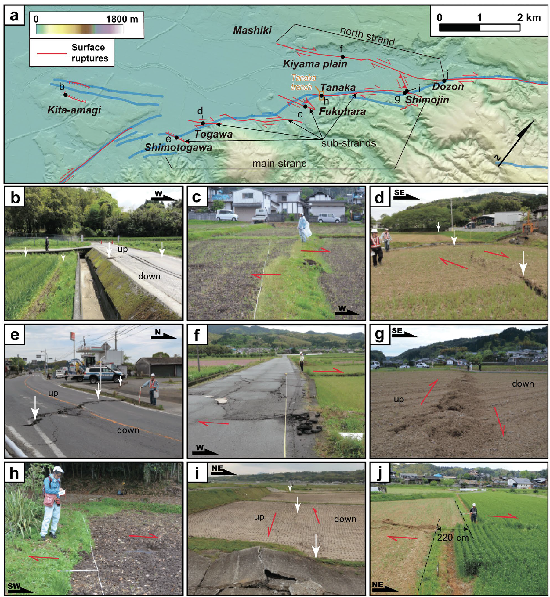
a Distribution of surface ruptures, previously mapped fault traces, and location of photographs (black dots) and the trench survey (yellow box) in the Uto segment and the southwestern section of the Futagawa segment of the Futagawa fault zone (Fig. 1c). b Surface rupture (white arrows) across a road and paddy field at Kitaamagi. c Surface rupture at Fukuhara showing dextral displacement of footpath in a paddy field (red half-arrows). d Left-stepping tension cracks showing a dextral slip in a wheat field at Togawa. e Surface rupture across a road at Shimotogawa with the north side downthrown by normal faulting with little lateral slip. f Surface ruptures on the north side of the Kiyama plain showing dextral offset of a road and paddy field. g Tensional cracks and mole track at Shimojin. The northwestern side of the wheat field was locally upthrown. h Dextral displacement at Tanaka along a surface rupture consistent with a fault trace exposed in previous trenching. i Surface rupture with sinistral and reverse offset at Shimojin, connecting two left-stepping en echelon dextral ruptures on the northern and southern edges of the Kiyama River alluvial plain. j Dextral displacement of a wheat field at Dozon, where the maximum slip of 220 cm was measured
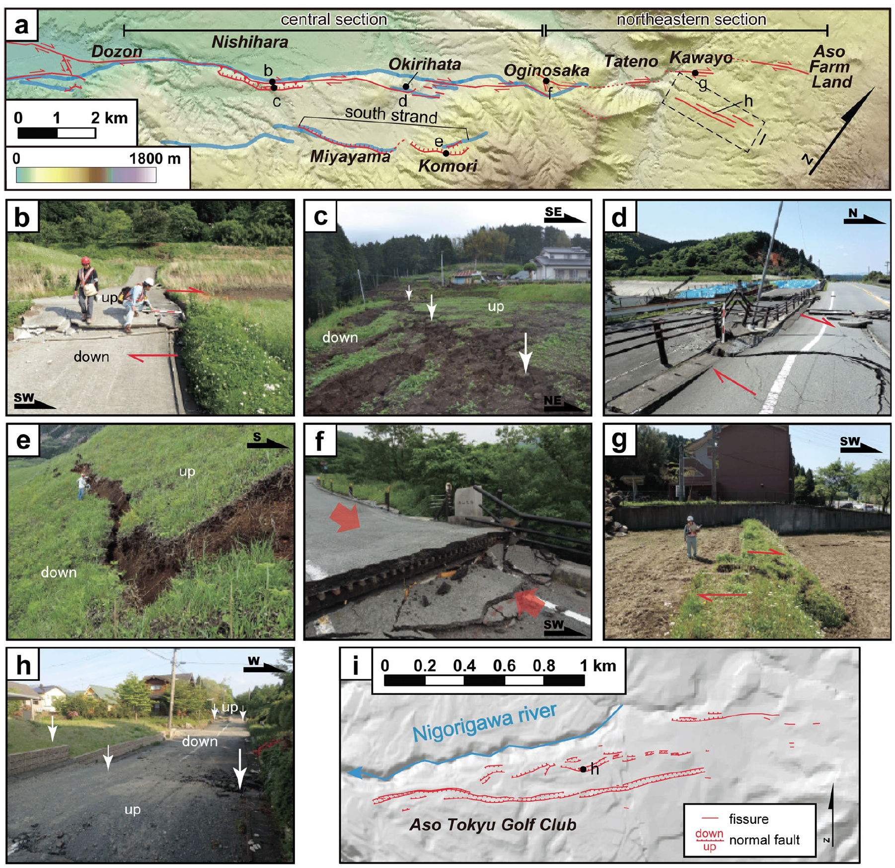
a Distribution of surface ruptures, previously mapped fault traces, and location of photographs (black dots) in the central and northeastern sections of the Futagawa segment of the Futagawa fault zone (Fig. 1C). b Surface rupture (red half-arrows) crossing a road at Nishihara. South side was upthrown and displaced to the southwest by reverse and dextral faulting. c Array of left-stepping tension cracks (white arrows) south of Nishihara related to dextral and normal faulting on the hillside. d Surface rupture crossing a road at the Okirihata dam showing dextral slip. e Surface rupture at Komori with the north side downthrown by normal faulting. f Surface rupture crossing the bridge at Oginosaka which was compressed by dextral faulting (red arrows). g Surface ruptures at Kawayo showing dextral offset of a field and footpath. h A small graben crossing a road, defined by surface ruptures in the foreground and background. i Surface ruptures and fissures (red lines) near the Nigorigawa River that defined small grabens
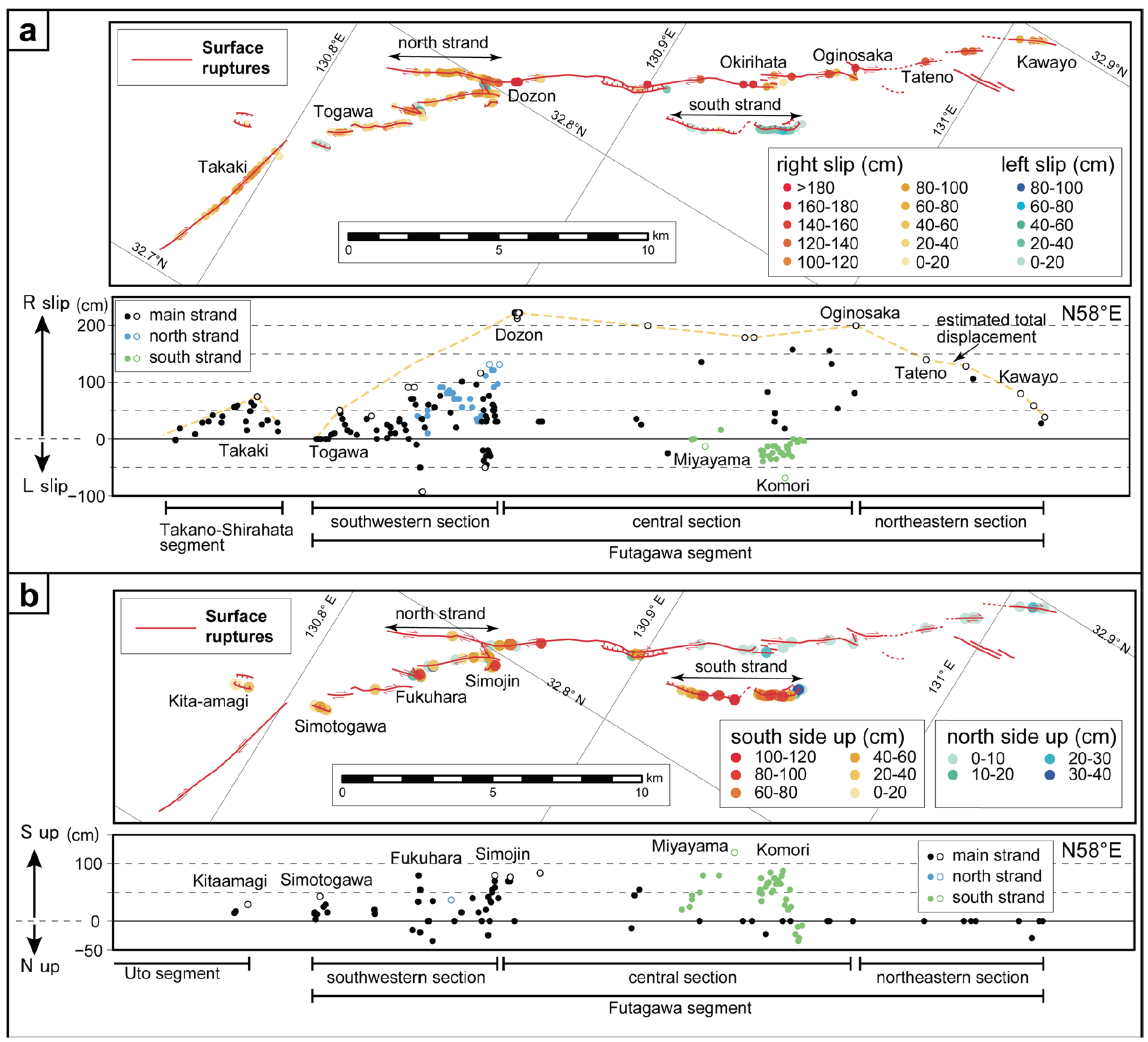
Distribution of the strike-slip component of surface ruptures (red lines) at measured locations (colored dots with the amount of displacement represented by their shade) along the Futagawa and Hinagu fault zones (top); explanation of surface ruptures in Fig. 1C. Diagram of slip distribution along the fault zone (bottom). Open dots show the representative displacement at each sub-strand. Dashed yellow line shows the estimated total displacement. b Distribution of the vertical component of surface ruptures along the Futagawa fault zone
- 2011.03.11 Summary of the M 9.0 Japan (Tohoku-Oki)
- 2026.07.28 M 6.8 Japan 352
- 2026.04.20 M 7.4 Japan 349
- 2025.12.08 M 7.6 Japan POSTER
- 2024.08.08 M 7.1 Japan
- 2024.01.01 M 7.5 Japan
- 2022.03.16 M 7.3 Japan
- 2018.09.05 M 6.6 Hokkaido, Japan
- 2016.07.29 M 7.7 Mariana
- 2016.11.21 M 6.9 Japan
- 2016.10.19 M 6.2 Japan
- 2016.08.20 M 6.0 Japan
- 2016.04.14 M 6.2 Japan
- 2016.04.01 M 6.0 Japan
- 2015.05.30 M 7.8 Izu Bonin
- 2015.05.31 M 7.8 Izu Bonin Update #1: triggered earthquakes
- 2015.05.31 M 7.8 Izu Bonin Update #2: Historic Seismicity
- 2015.06.09 M 7.8 Izu Bonin Update #3: seismic wave animations
- 2015.02.25 M 6.3 Japan (Sanriku Coast Update #5)
- 2015.02.21 M 6.7 Japan (Sanriku Coast Update #4)
- 2015.02.20 M 6.7 Japan (Sanriku Coast Update #3)
- 2015.02.16 M 6.7 Japan (Sanriku Coast Update #2)
- 2015.02.16 M 6.7 Japan (Sanriku Coast Update #1)
- 2015.02.16 M 6.7 Japan (Sanriku Coast)
- 2013.10.25 M 7.1 Japan (Honshu)
- 2011.03.11 M 9.0 Japan (Tohoku-Oki) Main Page
- 2011.03.11 M 9.0 Japan (Tōhoku-oki) Tsunami
- 2011.03.11 M 9.1 Japan (Tōhoku-oki) Decade Remembrance
- 1923.09.01 M 8.0 Kanto, Japan
Japan | Izu-Bonin | Mariana
General Overview
Earthquake Reports
Social Media
- Frisch, W., Meschede, M., Blakey, R., 2011. Plate Tectonics, Springer-Verlag, London, 213 pp.
- Hayes, G., 2018, Slab2 – A Comprehensive Subduction Zone Geometry Model: U.S. Geological Survey data release, https://doi.org/10.5066/F7PV6JNV.
- Holt, W. E., C. Kreemer, A. J. Haines, L. Estey, C. Meertens, G. Blewitt, and D. Lavallee (2005), Project helps constrain continental dynamics and seismic hazards, Eos Trans. AGU, 86(41), 383–387, , https://doi.org/10.1029/2005EO410002. /li>
- Jessee, M.A.N., Hamburger, M. W., Allstadt, K., Wald, D. J., Robeson, S. M., Tanyas, H., et al. (2018). A global empirical model for near-real-time assessment of seismically induced landslides. Journal of Geophysical Research: Earth Surface, 123, 1835–1859. https://doi.org/10.1029/2017JF004494
- Kreemer, C., J. Haines, W. Holt, G. Blewitt, and D. Lavallee (2000), On the determination of a global strain rate model, Geophys. J. Int., 52(10), 765–770.
- Kreemer, C., W. E. Holt, and A. J. Haines (2003), An integrated global model of present-day plate motions and plate boundary deformation, Geophys. J. Int., 154(1), 8–34, , https://doi.org/10.1046/j.1365-246X.2003.01917.x.
- Kreemer, C., G. Blewitt, E.C. Klein, 2014. A geodetic plate motion and Global Strain Rate Model in Geochemistry, Geophysics, Geosystems, v. 15, p. 3849-3889, https://doi.org/10.1002/2014GC005407.
- Meyer, B., Saltus, R., Chulliat, a., 2017. EMAG2: Earth Magnetic Anomaly Grid (2-arc-minute resolution) Version 3. National Centers for Environmental Information, NOAA. Model. https://doi.org/10.7289/V5H70CVX
- Müller, R.D., Sdrolias, M., Gaina, C. and Roest, W.R., 2008, Age spreading rates and spreading asymmetry of the world’s ocean crust in Geochemistry, Geophysics, Geosystems, 9, Q04006, https://doi.org/10.1029/2007GC001743
- Pagani,M. , J. Garcia-Pelaez, R. Gee, K. Johnson, V. Poggi, R. Styron, G. Weatherill, M. Simionato, D. Viganò, L. Danciu, D. Monelli (2018). Global Earthquake Model (GEM) Seismic Hazard Map (version 2018.1 – December 2018), DOI: 10.13117/GEM-GLOBAL-SEISMIC-HAZARD-MAP-2018.1
- Silva, V ., D Amo-Oduro, A Calderon, J Dabbeek, V Despotaki, L Martins, A Rao, M Simionato, D Viganò, C Yepes, A Acevedo, N Horspool, H Crowley, K Jaiswal, M Journeay, M Pittore, 2018. Global Earthquake Model (GEM) Seismic Risk Map (version 2018.1). https://doi.org/10.13117/GEM-GLOBAL-SEISMIC-RISK-MAP-2018.1
- Storchak, D. A., D. Di Giacomo, I. Bondár, E. R. Engdahl, J. Harris, W. H. K. Lee, A. Villaseñor, and P. Bormann (2013), Public release of the ISC-GEM global instrumental earthquake catalogue (1900–2009), Seismol. Res. Lett., 84(5), 810–815, doi:10.1785/0220130034.
- Zhu, J., Baise, L. G., Thompson, E. M., 2017, An Updated Geospatial Liquefaction Model for Global Application, Bulletin of the Seismological Society of America, 107, p 1365-1385, https://doi.org/0.1785/0120160198
- An’naka, T., K. Inagaki, H. Tanaka, and K. Yanagisawa (2003), Characteristics of great earthquakes along the Nankai trough based on numerical tsunami simulation, J. Earthquake Eng. [CD‐ROM], 27, article 307.
- Chapman et al., 2009. Development of Methodologies for the Identification of Volcanic and Tectonic Hazards to Potential HLW Repository Sites in Japan –The Kyushu Case Study-, NUMO-TR-09-02, NOv. 2009, 192 pp.
- Furumura, T., K. Imai, and T. Maeda (2011), A revised tsunami source model for the 1707 Hoei earthquake and simulation of tsunami inundation of Ryujin Lake, Kyushu, Japan, J. Geophys. Res., 116, B02308, https://doi.org/10.1029/2010JB007918
- Garrett, E., O. Fujiwara, P. Garrett, V. M. A. Heyvaert, M. Shishikura, Y. Yokoyama, A. Hubert-Ferrari, H. Brückner, A. Nakamura, and M. De Batist, 2016. A systematic review of geological evidence for Holocene earthquakes and tsunamis along the Nankai-Suruga Trough, Japan, Earth-Science Reviews 159, 337–357, doi: 10.1016/j.earscirev.2016.06.011.
- Goltz, J. D., K. Yamori, K. Nakayachi, H. Shiroshita, T. Sugiyama, and Y. Matsubara, 2024. Operational Earthquake Forecasting in Japan: A Study of Municipal Government Planning for an Earthquake Advisory or Warning in the Nankai Region, Seismological Research Letters 95, no. 4, 2251–2265, doi: 10.1785/0220230304.
- Hyodo, M., T. Hori, and Y. Kaneda, 2016. A possible scenario for earlier occurrence of the next Nankai earthquake due to triggering by an earthquake at Hyuga-nada, off southwest Japan, Earth Planet Sp 68, no. 1, 6, doi: 10.1186/s40623-016-0384-6.
- Ichinose, G. A., H. K. Thio, P. G. Somerville, T. Sato, and T. Ishii, Rupture process of the 1944 Tonankai earthquake (Ms 8.1) from the inversion of teleseismic and regional seismograms, J. Geophys. Res., 108(B10), 2497, doi:10.1029/2003JB002393, 2003.
- Kurikami et al., 2009. Study on strategy and methodology for repository concept development for the Japanese geological disposal project, NUMO-TR-09-04, Sept. 20-09, 101 pp.
- Moore, G.F., Bangs, N.L., Taira, A., Kuramoto, S., Pangborn, E., and Tobin, H.J., 2007. Three-Dimensional Splay Fault Geometry and Implications for Tsunami Generation in Science, v. 318, p. 1128-1131.
- 1Moore, G.F., Park, J.-O., Bangs, N.L., Gulick, S.P., Tobin, H.J., Nakamura, Y., Sato, S., Tsuji, T., Yoro, T., Tanaka, H., Uraki, S., Kido, Y., Sanada, Y., Kuramoto, S., and Taira, A., 2009. Structural and seismic stratigraphic framework of the NanTroSEIZE Stage 1 transect. In Kinoshita, M., Tobin, H., Ashi, J., Kimura, G., Lallemant, S., Screaton, E.J., Curewitz, D., Masago, H., Moe, K.T., and the Expedition 314/315/316 Scientists, Proc. IODP, 314/315/316: Washington, DC (Integrated Ocean Drilling Program Management International, Inc.). doi:10.2204/iodp.proc.314315316.102.2009
- Rhea, S., Tarr, A.C., Hayes, G., Villaseñor, A., and Benz, H.M., 2010. Seismicity of the earth 1900–2007, Japan and vicinity: U.S. Geological Survey Open-File Report 2010–1083-D, scale 1:6,000,000.
- Toda, S., Stein, R. S., and Sevilgen, V., 2024. Japan’s magnitude 7.1 shock triggers megaquake warning. How likely is this scenario?, Temblor, http://doi.org/10.32858/temblor.348
- Van Horne, A., Sato, H., Ishiyama, T., 2017. Evolution of the Sea of Japan back-arc and some unsolved issues in Tectonophysics, v. 710-711, p. 6-20, http://dx.doi.org/10.1016/j.tecto.2016.08.020
- Yagi, Y., M. Kikuchi, S. Yoshida, and T. Sagiya, 1999. Comparison of the coseismic rupture with the aftershock distribution in the Hyuga-nada Earthquakes of 1996, Geophysical Research Letters 26, no. 20, 3161–3164, doi: 10.1029/1999GL005340
References:
Basic & General References
Specific References
Return to the Earthquake Reports page.
- Sorted by Magnitude
- Sorted by Year
- Sorted by Day of the Year
- Sorted By Region