I don’t always have the time to write a proper Earthquake Report. However, I prepare interpretive posters for these events.
Because of this, I present Earthquake Report Lite. (but it is more than just water, like the adult beverage that claims otherwise). I will try to describe the figures included in the poster, but sometimes I will simply post the poster here.
There was a magnitude M 7.6 earthquake in Mexico on 19 September 2022.
https://earthquake.usgs.gov/earthquakes/eventpage/us7000i9bw/executive
I am catching up on some Earthquake Reports that I did not yet post since my website was being migrated to a more secure and reliable server (and more expensive).
The tectonics of coastal southwestern Mexico is dominated by the convergent plate boundary between the Cocos plate (to the southwest) and the North America plate (to the northeast). Here, the Cocos plate subducts below (goes underneath) the North America plate.
The fault between these plates is called a megathrust subduction zone fault and the plate boundary forms the Middle America trench.
This M 7.6 earthquake mechanism (the “moment tensor”) shows that this event was a compressional earthquake (reverse or thrust).
Based on it’s location, the event probably happened along the megathrust fault.
This earthquake even generated a tsunami recorded on tide gages in the region!
Below is my interpretive poster for this earthquake
- I plot the seismicity from the past month, with diameter representing magnitude (see legend). I include earthquake epicenters from 1921-2021 with magnitudes M ≥ 3.0 in one version.
- I plot the USGS fault plane solutions (moment tensors in blue and focal mechanisms in orange), possibly in addition to some relevant historic earthquakes.
- A review of the basic base map variations and data that I use for the interpretive posters can be found on the Earthquake Reports page. I have improved these posters over time and some of this background information applies to the older posters.
- Some basic fundamentals of earthquake geology and plate tectonics can be found on the Earthquake Plate Tectonic Fundamentals page.
- In the upper left corner is a map that shows the plates, their boundaries, and a century of seismicity.
- In the upper right are two maps that show models of how there may have been landslides or liquefaction because of the earthquake shaking and impacts. Read more about landslides and liquefaction here. I include the USGS epicenter as a red circle. However, these ground failure models are based on the USGS epicenter/location.
- On the center right is a map that shows the historic subduction zone earthquake history for the subduction zone offshore of Mexico (National Seismological Service of Mexico).
- To the left of those two maps is a low angle oblique view of the tectonic plates and how they are oriented relative to each other (Manea et al., 2013).
- In the lower right corner is a map that shows the ground shaking from the earthquake, with color representing intensity using the Modified Mercalli Intensity (MMI) scale. The closer to the earthquake, the stronger the ground shaking. The colors on the map represent the USGS model of ground shaking. The colored circles represent reports from people who posted information on the USGS Did You Feel It? part of the website for this earthquake. There are things that affect the strength of ground shaking other than distance, which is why the reported intensities are different from the modeled intensities.
- On the left, below the tectonic setting map is a plot that shows how the shaking intensity models and reports relate to each other. The horizontal axis is distance from the earthquake and the vertical axis is shaking intensity (using the MMI scale, just like in the map to the right: these are the same datasets).
- In the upper left-center is a figure that shows the USGS earthquake slip model. This shows how much the fault slipped in different areas (based on their modeling, not observation). The model shows that there were places that may have slipped over 1.25 meters (~4 feet).
- In the lower left is a series of plots from the tide gages in the region. The location of these gages are shown on the main map. The tsunami wave height (vertical distance between the peak of the wave and the trough of the wave) ranged from 0.6m to 1.7m.
I include some inset figures.
- Here is the map with 3 month’s seismicity plotted.

- I could not help myself. I am so excited to have this website back up and running, like a fully operational space station, that I include below some additional figures that help us understand the tectonic setting.
- Here is the low angle oblique view of this tectonic region (Manea et al., 2013).
- Here are the plots from the tide gages operated in the region.
- These tide gages are organized north to south, top to bottom.
- The dark blue line is the tidal forecast. The medium blue line is the tide gage record. The light blue line is the tide gage record minus the tidal forecast (basically the tsunami plus any other influence (like atmospheric pressure influences, or storm surge, etc.).
- The locations for these gages are labeled on the interpretive poster above.
- The earthquake origin time is labeled in orange.
- Time is presented in UTC.
- Here is tectonic map from Franco et al. (2012).
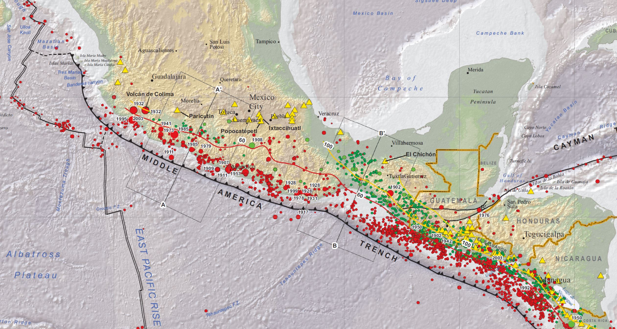
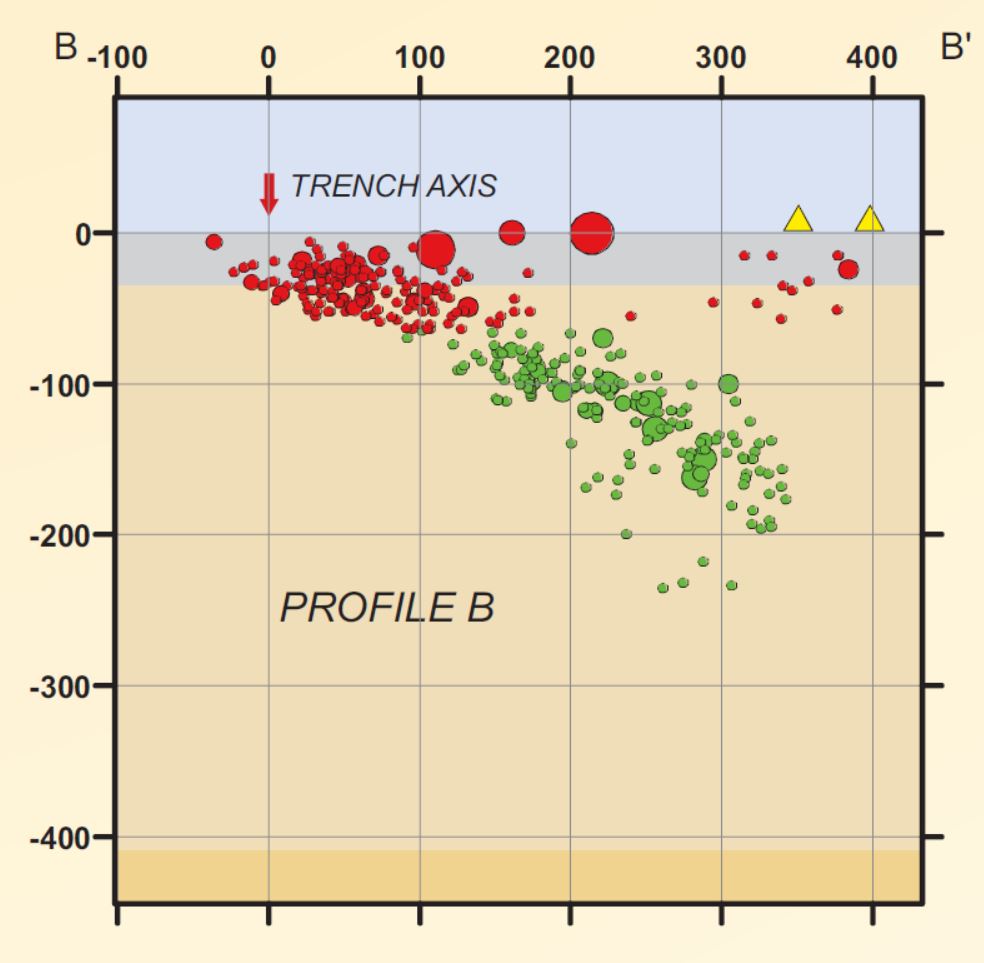
- These figures are from the USGS publication (Benz et al., 2011) that presents an educational poster about the historic seismicity and seismic hazard along the Middle America Trench.
- First is a map showing earthquake depth as color (green depth > red). Seismicity cross section B-B’ is shown on the map. Today’s M=6.6 quake is nearest this section.
- Here is a map from Benz et al. (2011) that shows the seismic hazard for this region.
- Here are some figures from Manea et al. (2013). First are the map and low angle oblique view of the Cocos plate.
- Here is a map showing the spreading ridge features, along with the plate boundary faults (Mann, 2007). This is similar to the inset map in the interpretive poster.
- Here is the McCann et al. (1979) summary figure, showing the earthquake history of the region.
- This is a more updated figure from Franco et al. (2005) showing the seismic gap.
- Here is a map from Franco et al. (2015) that shows the rupture patches for historic earthquakes in this region.
Supportive Figures
Development of the Tepic–Zacoalco (TZ), Colima, and Chapala rifts. The TZ rift is formed by the Rivera slab rollback, enhanced by the toroidal flow around the slab edges. The Colima rift is probably related with the oblique convergence between Rivera and NAM plates at ~5 Ma.
Tectonic setting of the Caribbean Plate. Grey rectangle shows study area of Fig. 2. Faults are mostly from Feuillet et al. (2002). PMF, Polochic–Motagua faults; EF, Enriquillo Fault; TD, Trinidad Fault; GB, Guatemala Basin. Topography and bathymetry are from Shuttle Radar Topography Mission (Farr&Kobrick 2000) and Smith & Sandwell (1997), respectively. Plate velocities relative to Caribbean Plate are from Nuvel1 (DeMets et al. 1990) for Cocos Plate, DeMets et al. (2000) for North America Plate and Weber et al. (2001) for South America Plate.


A. Geodynamic and tectonic setting alongMiddle America Subduction Zone. JB: Jalisco Block; Ch. Rift—Chapala rift; Co. rift—Colima rift; EGG—El Gordo Graben; EPR: East Pacific Rise; MCVA: Modern Chiapanecan Volcanic Arc; PMFS: Polochic–Motagua Fault System; CR—Cocos Ridge. Themain Quaternary volcanic centers of the TransMexican Volcanic Belt (TMVB) and the Central American Volcanic Arc (CAVA) are shown as blue and red dots, respectively. B. 3-D view of the Pacific, Rivera and Cocos plates’ bathymetrywith geometry of the subducted slab and contours of the depth to theWadati–Benioff zone (every 20 km). Grey arrows are vectors of the present plate convergence along theMAT. The red layer beneath the subducting plate represents the sub-slab asthenosphere.
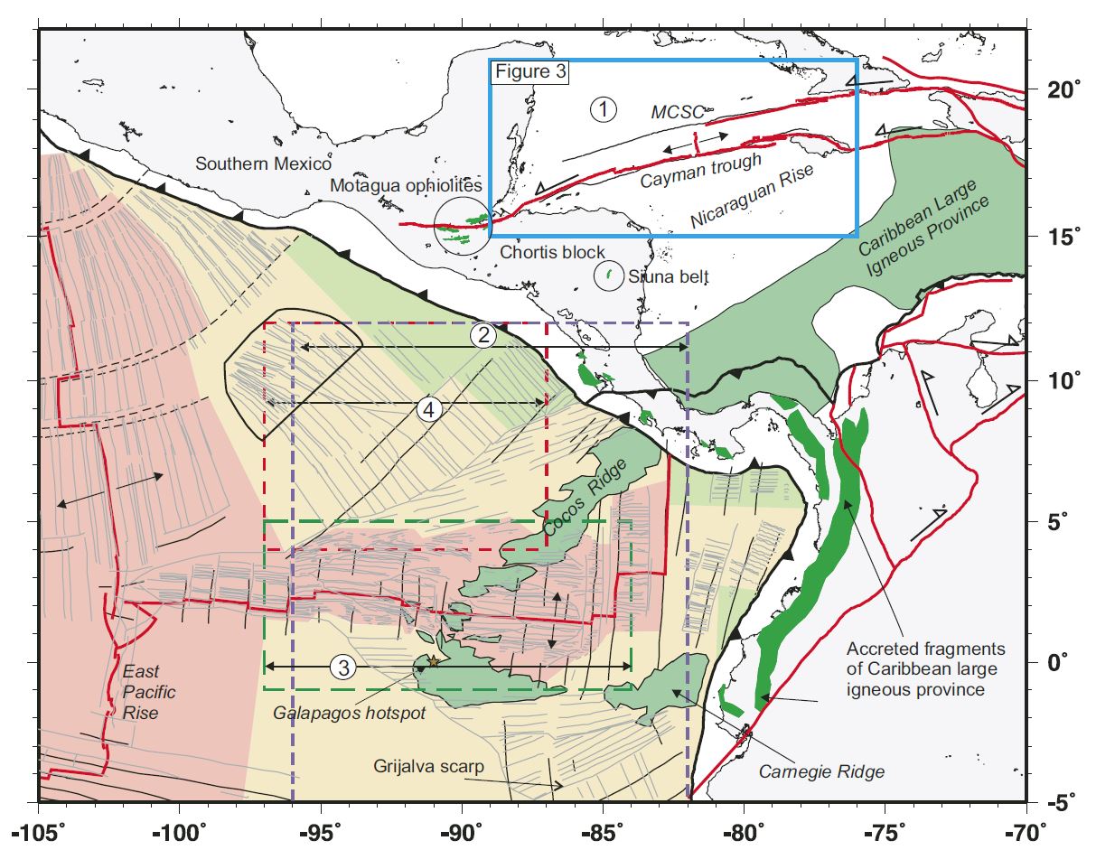
Marine magnetic anomalies and fracture zones that constrain tectonic reconstructions such as those shown in Figure 4 (ages of anomalies are keyed to colors as explained in the legend; all anomalies shown are from University of Texas Institute for Geophysics PLATES [2000] database): (1) Boxed area in solid blue line is area of anomaly and fracture zone picks by Leroy et al. (2000) and Rosencrantz (1994); (2) boxed area in dashed purple line shows anomalies and fracture zones of Barckhausen et al. (2001) for the Cocos plate; (3) boxed area in dashed green line shows anomalies and fracture zones from Wilson and Hey (1995); and (4) boxed area in red shows anomalies and fracture zones from Wilson (1996). Onland outcrops in green are either the obducted Cretaceous Caribbean large igneous province, including the Siuna belt, or obducted ophiolites unrelated to the large igneous province (Motagua ophiolites). The magnetic anomalies and fracture zones record the Cenozoic relative motions of all divergent plate pairs infl uencing the Central American subduction zone (Caribbean, Nazca, Cocos, North America, and South America). When incorporated into a plate model, these anomalies and fracture zones provide important constraints on the age and thickness of subducted crust, incidence angle of subduction, and rate of subduction for the Central American region. MCSC—Mid-Cayman Spreading Center.
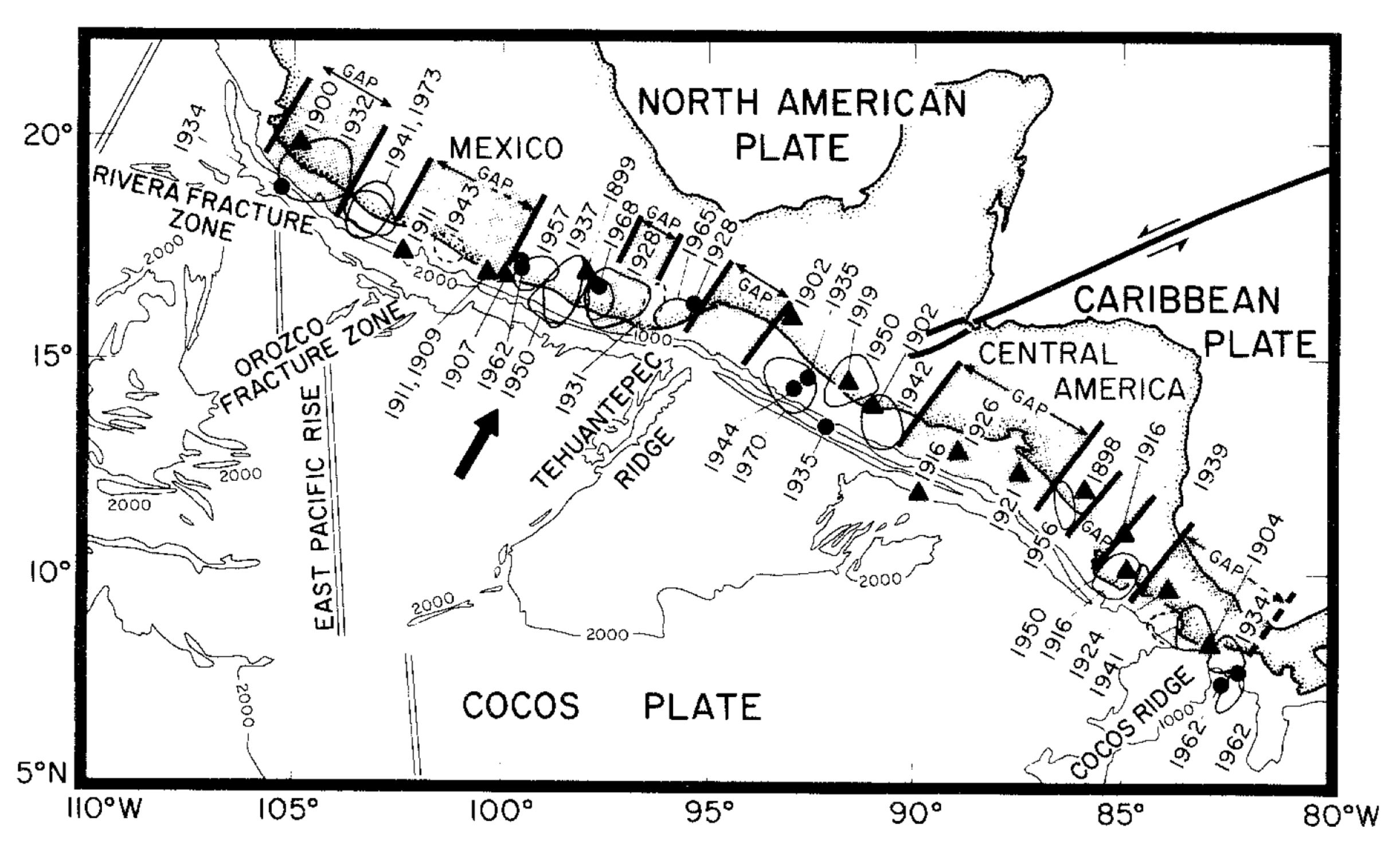
Rupture zones (ellipses) and epicenters (triangles and circles) of large shallow earthquakes (after KELLEHER et al., 1973) and bathymetry (CHASE et al., 1970) along the Middle America arc. Note that six gaps which have earthquake histories have not ruptured for 40 years or more. In contrast, the gap near the intersection of the Tehuantepec ridge has no known history of large shocks. Contours are in fathoms.

The study area encompasses Guerrero and Oaxaca states of Mexico. Shaded ellipse-like areas annotated with the years are rupture areas of the most recent major thrust earthquakes (M≥6.5) in the Mexican subduction zone. Triangles show locations of permanent GPS stations. Small hexagons indicate campaign GPS sites. Arrows are the Cocos-North America convergence vectors from NUVEL-1A model (DeMets et al., 1994). Double head arrow shows the extent of the Guerrero seismic gap. Solid and dashed curves annotated with negative numbers show the depth in km down to the surface of subducting Cocos plate (modified from Pardo and Su´arez, 1995, using the plate interface configuration model for the Central Oaxaca from this study, the model for Guerrero from Kostoglodov et al. (1996), and the last seismological estimates in Chiapas by Bravo et al. (2004). MAT, Middle America trench.
- There are many different ways in which a landslide can be triggered. The first order relations behind slope failure (landslides) is that the “resisting” forces that are preventing slope failure (e.g. the strength of the bedrock or soil) are overcome by the “driving” forces that are pushing this land downwards (e.g. gravity). The ratio of resisting forces to driving forces is called the Factor of Safety (FOS). We can write this ratio like this:
FOS = Resisting Force / Driving Force
- When FOS > 1, the slope is stable and when FOS < 1, the slope fails and we get a landslide. The illustration below shows these relations. Note how the slope angle α can take part in this ratio (the steeper the slope, the greater impact of the mass of the slope can contribute to driving forces). The real world is more complicated than the simplified illustration below.
- Landslide ground shaking can change the Factor of Safety in several ways that might increase the driving force or decrease the resisting force. Keefer (1984) studied a global data set of earthquake triggered landslides and found that larger earthquakes trigger larger and more numerous landslides across a larger area than do smaller earthquakes. Earthquakes can cause landslides because the seismic waves can cause the driving force to increase (the earthquake motions can “push” the land downwards), leading to a landslide. In addition, ground shaking can change the strength of these earth materials (a form of resisting force) with a process called liquefaction.
- Sediment or soil strength is based upon the ability for sediment particles to push against each other without moving. This is a combination of friction and the forces exerted between these particles. This is loosely what we call the “angle of internal friction.” Liquefaction is a process by which pore pressure increases cause water to push out against the sediment particles so that they are no longer touching.
- An analogy that some may be familiar with relates to a visit to the beach. When one is walking on the wet sand near the shoreline, the sand may hold the weight of our body generally pretty well. However, if we stop and vibrate our feet back and forth, this causes pore pressure to increase and we sink into the sand as the sand liquefies. Or, at least our feet sink into the sand.
- Below is a diagram showing how an increase in pore pressure can push against the sediment particles so that they are not touching any more. This allows the particles to move around and this is why our feet sink in the sand in the analogy above. This is also what changes the strength of earth materials such that a landslide can be triggered.
- Below is a diagram based upon a publication designed to educate the public about landslides and the processes that trigger them (USGS, 2004). Additional background information about landslide types can be found in Highland et al. (2008). There was a variety of landslide types that can be observed surrounding the earthquake region. So, this illustration can help people when they observing the landscape response to the earthquake whether they are using aerial imagery, photos in newspaper or website articles, or videos on social media. Will you be able to locate a landslide scarp or the toe of a landslide? This figure shows a rotational landslide, one where the land rotates along a curvilinear failure surface.
- Here is an excellent educational video from IRIS and a variety of organizations. The video helps us learn about how earthquake intensity gets smaller with distance from an earthquake. The concept of liquefaction is reviewed and we learn how different types of bedrock and underlying earth materials can affect the severity of ground shaking in a given location. The intensity map above is based on a model that relates intensity with distance to the earthquake, but does not incorporate changes in material properties as the video below mentions is an important factor that can increase intensity in places.
- If we look at the map at the top of this report, we might imagine that because the areas close to the fault shake more strongly, there may be more landslides in those areas. This is probably true at first order, but the variation in material properties and water content also control where landslides might occur.
- There are landslide slope stability and liquefaction susceptibility models based on empirical data from past earthquakes. The USGS has recently incorporated these types of analyses into their earthquake event pages. More about these USGS models can be found on this page.
Earthquake Triggered Landslides


Social Media:
#EarthquakeReport for the M 7.6 (likely) subduction zone #Earthquake in #Mexico on 19 Sept 2022
catching up on reports that happened after my website went down
generated 0.6-1.7m wave height #Tsunami
probably triggered landslides/induced liquefactionhttps://t.co/9zpN2ZlAhw pic.twitter.com/tMDb4mSwCw— Jason "Jay" R. Patton (@patton_cascadia) November 9, 2022
- 2022.09.19 M 7.6 Mexico
- 2021.09.08 M 7.0 Mexico
- 2021.07.21 M 6.7 Panama
- 2020.06.23 M 7.4 Mexico
- 2019.02.01 M 6.6 Guatemala & Mexico
- 2018.02.16 M 7.2 Oaxaca, Mexico
- 2018.01.19 M 6.3 Gulf of California
- 2017.09.19 M 7.1 Puebla, Mexico
- 2017.09.19 M 7.1 Puebla, Mexico Update #1
- 2017.09.08 M 8.1 Chiapas, Mexico
- 2017.09.08 M 8.1 Chiapas, Mexico Update #1
- 2017.09.23 M 8.1 Chiapas, Mexico Update #2
- 2017.06.22 M 6.8 Guatemala
- 2017.06.14 M 6.9 Guatemala
- 2017.05.12 M 6.2 El Salvador
- 2017.03.29 M 5.7 Gulf of California
- 2016.11.24 M 7.0 El Salvador
- 2016.04.29 M 6.6 East Pacific Rise / MAT
- 2016.01.21 M 6.6 Mexico
- 2015.09.13 M 6.6 Gulf California
- 2015.09.13 M 6.6 Gulf California Update #1
- 2015.01.07 M 6.6 Panama
- 2015.01.31 M 5.5 Panama Update #1
- 2014.05.13 M 6.5 Panama
- 2014.05.13 M 6.5 Panama Update #1
- 2014.10.14 M 7.3 El Salvador
- 2013.10.20 M 6.4 Gulf California
Mexico | Central America
General Overview
Earthquake Reports
- Frisch, W., Meschede, M., Blakey, R., 2011. Plate Tectonics, Springer-Verlag, London, 213 pp.
- Hayes, G., 2018, Slab2 – A Comprehensive Subduction Zone Geometry Model: U.S. Geological Survey data release, https://doi.org/10.5066/F7PV6JNV.
- Holt, W. E., C. Kreemer, A. J. Haines, L. Estey, C. Meertens, G. Blewitt, and D. Lavallee (2005), Project helps constrain continental dynamics and seismic hazards, Eos Trans. AGU, 86(41), 383–387, , https://doi.org/10.1029/2005EO410002. /li>
- Jessee, M.A.N., Hamburger, M. W., Allstadt, K., Wald, D. J., Robeson, S. M., Tanyas, H., et al. (2018). A global empirical model for near-real-time assessment of seismically induced landslides. Journal of Geophysical Research: Earth Surface, 123, 1835–1859. https://doi.org/10.1029/2017JF004494
- Kreemer, C., J. Haines, W. Holt, G. Blewitt, and D. Lavallee (2000), On the determination of a global strain rate model, Geophys. J. Int., 52(10), 765–770.
- Kreemer, C., W. E. Holt, and A. J. Haines (2003), An integrated global model of present-day plate motions and plate boundary deformation, Geophys. J. Int., 154(1), 8–34, , https://doi.org/10.1046/j.1365-246X.2003.01917.x.
- Kreemer, C., G. Blewitt, E.C. Klein, 2014. A geodetic plate motion and Global Strain Rate Model in Geochemistry, Geophysics, Geosystems, v. 15, p. 3849-3889, https://doi.org/10.1002/2014GC005407.
- Meyer, B., Saltus, R., Chulliat, a., 2017. EMAG2: Earth Magnetic Anomaly Grid (2-arc-minute resolution) Version 3. National Centers for Environmental Information, NOAA. Model. https://doi.org/10.7289/V5H70CVX
- Müller, R.D., Sdrolias, M., Gaina, C. and Roest, W.R., 2008, Age spreading rates and spreading asymmetry of the world’s ocean crust in Geochemistry, Geophysics, Geosystems, 9, Q04006, https://doi.org/10.1029/2007GC001743
- Pagani,M. , J. Garcia-Pelaez, R. Gee, K. Johnson, V. Poggi, R. Styron, G. Weatherill, M. Simionato, D. Viganò, L. Danciu, D. Monelli (2018). Global Earthquake Model (GEM) Seismic Hazard Map (version 2018.1 – December 2018), DOI: 10.13117/GEM-GLOBAL-SEISMIC-HAZARD-MAP-2018.1
- Silva, V ., D Amo-Oduro, A Calderon, J Dabbeek, V Despotaki, L Martins, A Rao, M Simionato, D Viganò, C Yepes, A Acevedo, N Horspool, H Crowley, K Jaiswal, M Journeay, M Pittore, 2018. Global Earthquake Model (GEM) Seismic Risk Map (version 2018.1). https://doi.org/10.13117/GEM-GLOBAL-SEISMIC-RISK-MAP-2018.1
- Zhu, J., Baise, L. G., Thompson, E. M., 2017, An Updated Geospatial Liquefaction Model for Global Application, Bulletin of the Seismological Society of America, 107, p 1365-1385, https://doi.org/0.1785/0120160198
- Franco, A., C. Lasserre H. Lyon-Caen V. Kostoglodov E. Molina M. Guzman-Speziale D. Monterosso V. Robles C. Figueroa W. Amaya E. Barrier L. Chiquin S. Moran O. Flores J. Romero J. A. Santiago M. Manea V. C. Manea, 2012. Fault kinematics in northern Central America and coupling along the subduction interface of the Cocos Plate, from GPS data in Chiapas (Mexico), Guatemala and El Salvador in Geophysical Journal International., v. 189, no. 3, p. 1223-1236. DOI: https://doi.org/10.1111/j.1365-246X.2012.05390.x
- Franco, S.I., Kostoglodov, V., Larson, K.M., Manea, V.C>, Manea, M., and Santiago, J.A., 2005. Propagation of the 2001–2002 silent earthquake and interplate coupling in the Oaxaca subduction zone, Mexico in Earth Planets Space, v. 57., p. 973-985.
- Garcia-Casco, A., Projenza, J.A., Iturralde-Vinent, M.A., 2011. Subduction Zones of the Caribbean: the sedimentary, magmatic, metamorphic and ore-deposit records UNESCO/iugs igcp Project 546 Subduction Zones of the Caribbean in Geologica Acta, v. 9, no., 3-4, p. 217-224
- Benz, H.M., Dart, R.L., Villaseñor, Antonio, Hayes, G.P., Tarr, A.C., Furlong, K.P., and Rhea, Susan, 2011 a. Seismicity of the Earth 1900–2010 Mexico and vicinity: U.S. Geological Survey Open-File Report 2010–1083-F, scale 1:8,000,000.
- Franco, A., Lasserre, C., Lyon-Caen, H., Kostoglodov, V., Molina, E., Guzman-Speziale, M., Monterosso, D., Robles, V., Figueroa, C., Amaya, W., Barrier, E., Chiquin, L., Moran, S., Flores, O., Romero, J., Santiago, J.A., Manea, M., Manea, V.C., 2012. Fault kinematics in northern Central America and coupling along the subduction interface of the Cocos Plate, from GPS data in Chiapas (Mexico), Guatemala and El Salvador in Geophysical Journal International., v. 189, no. 3, p. 1223-1236 https://doi.org/10.1111/j.1365-246X.2012.05390.x
- Manea, V.C., et al., 2013. A geodynamical perspective on the subduction of Cocos and Rivera plates beneath Mexico and Central America in Tectonophysics, http://dx.doi.org/10.1016/j.tecto.2012.12.039
- Manea, M., and Manea, V.C., 2014. On the origin of El Chichón volcano and subduction of Tehuantepec Ridge: A geodynamical perspective in JGVR, v. 175, p. 459-471.
- Mann, P., 2007. Overview of the tectonic history of northern Central America, in Mann, P., ed., Geologic and tectonic development of the Caribbean plate boundary in northern Central America: Geological Society of America Special Paper 428, p. 1–19, doi: 10.1130/2007.2428(01). For
- McCann, W.R., Nishenko S.P., Sykes, L.R., and Krause, J., 1979. Seismic Gaps and Plate Tectonics” Seismic Potential for Major Boundaries in Pageoph, v. 117
References:
Basic & General References
Specific References
Return to the Earthquake Reports page.
- Sorted by Magnitude
- Sorted by Year
- Sorted by Day of the Year
- Sorted By Region