The earthquakes continue, every day. Today, there was a large earthquake associated with the subduction zone that forms the Kermadec Trench.
This earthquake was quite deep, so was not expected to generate a significant tsunami (if one at all).
There are several analogies to today’s earthquake. There was a M 7.4 earthquake in a similar location, but much deeper. These are an interesting comparison because the M 7.4 was compressional and the M 6.9 was extensional. There is some debate about what causes ultra deep earthquakes. The earthquakes that are deeper than about 40-50 km are not along subduction zone faults, but within the downgoing plate. This M 6.9 appears to be in a part of the plate that is bending (based on the Benz et al., 2011 cross section). As plates bend downwards, the upper part of the plate gets extended and the lower part of the plate experiences compression.
This is my first earthquake report to utilize the new slab contours (Slab 2.0) from Hayes (2018).
There has been a recent sequence of ultra deep earthquakes in the Fiji region, as well as subduction zone related earthquakes along the southern New Hebrides Trench. These links lead to my earthquake reports for those two regions: Fiji and New Hebrides.
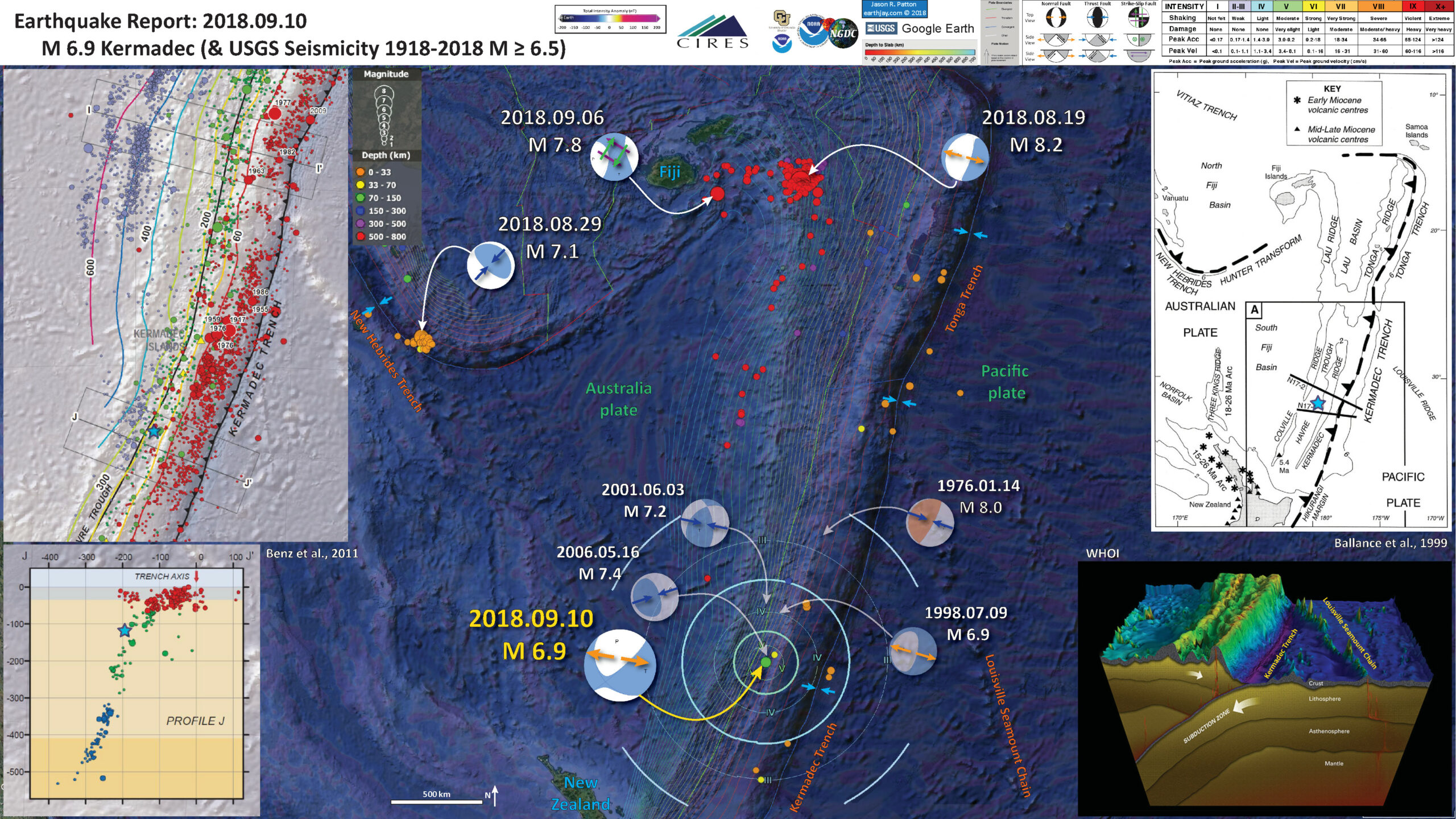
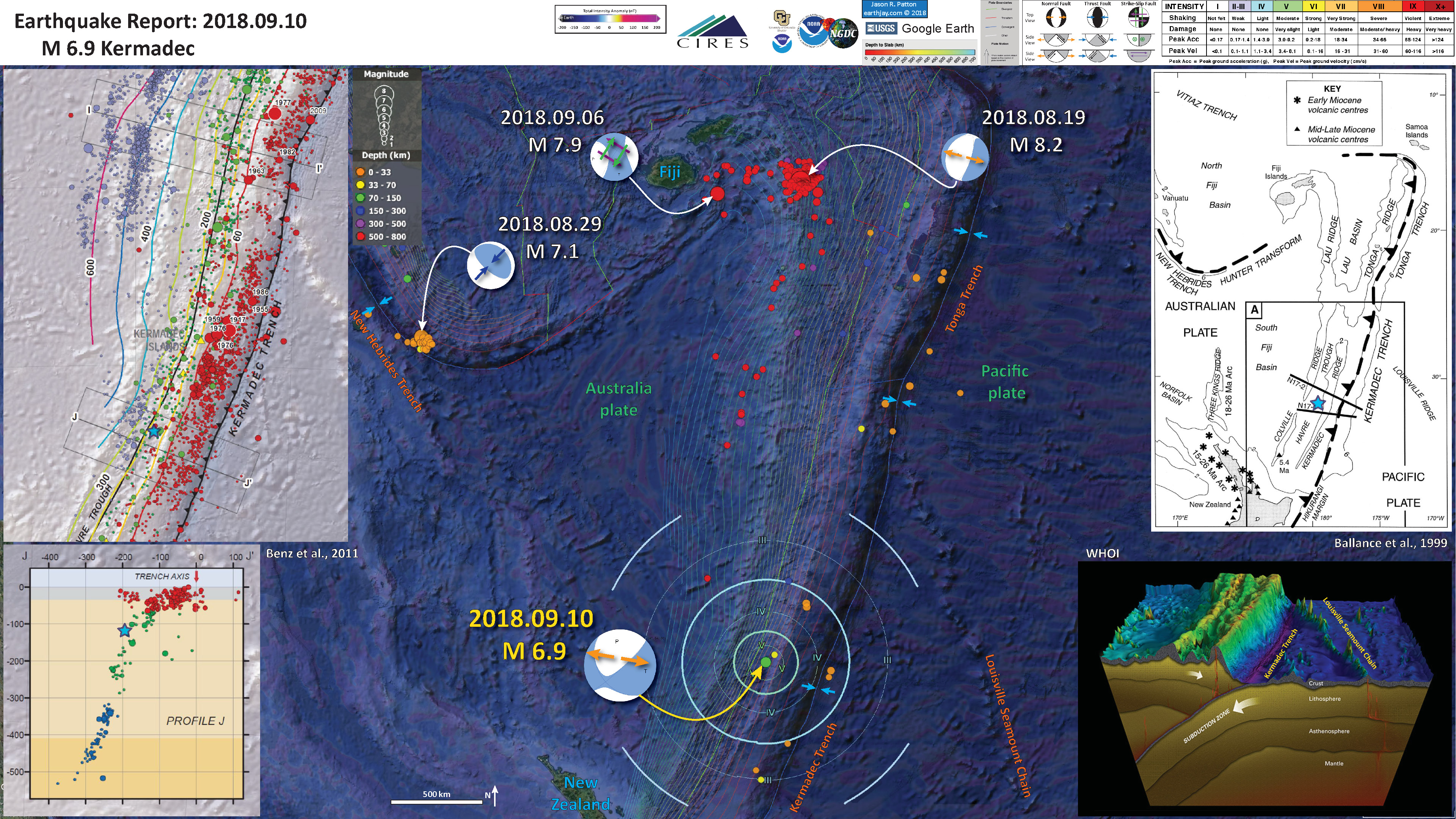
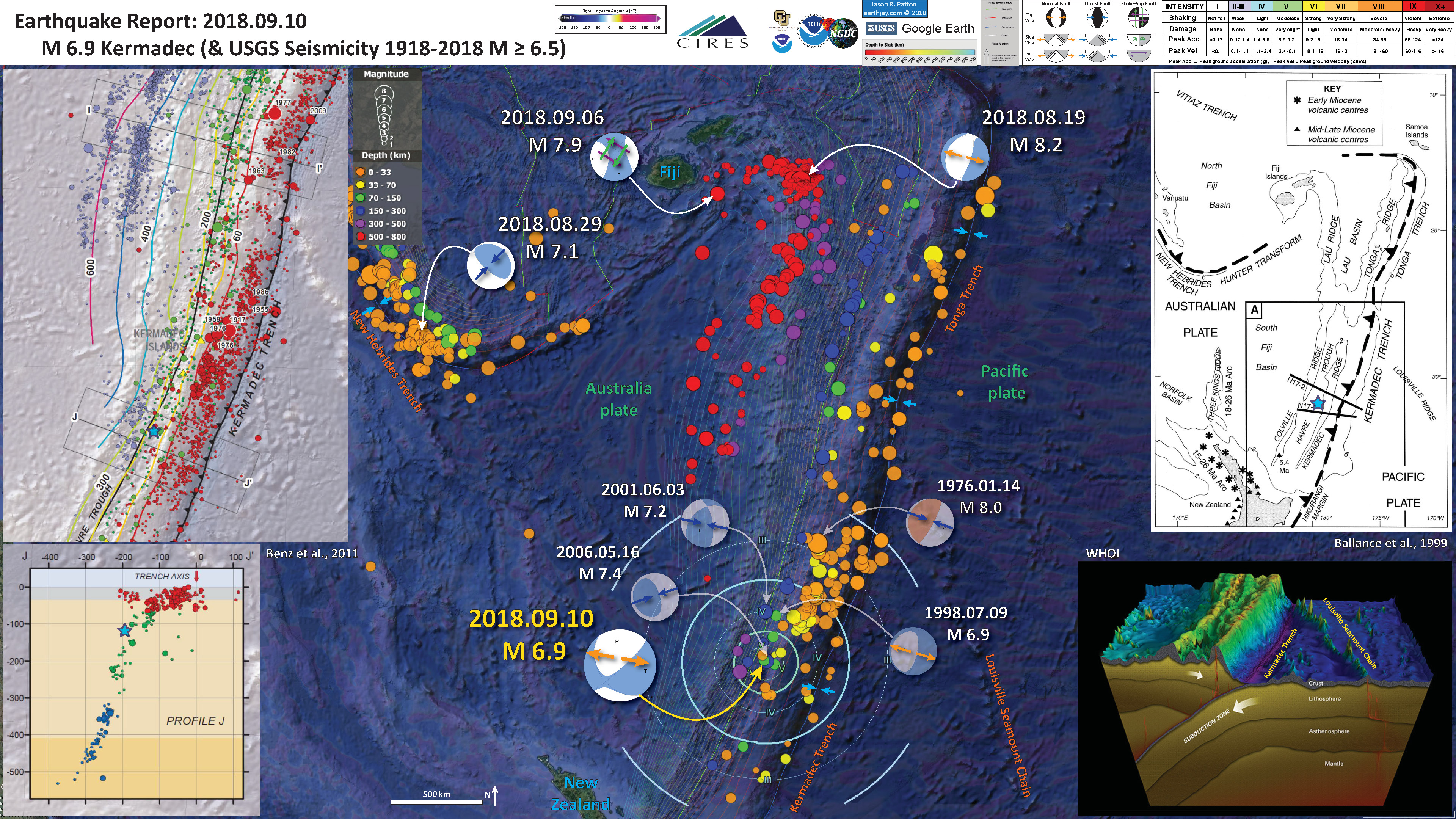
Below is my interpretive poster for this earthquake
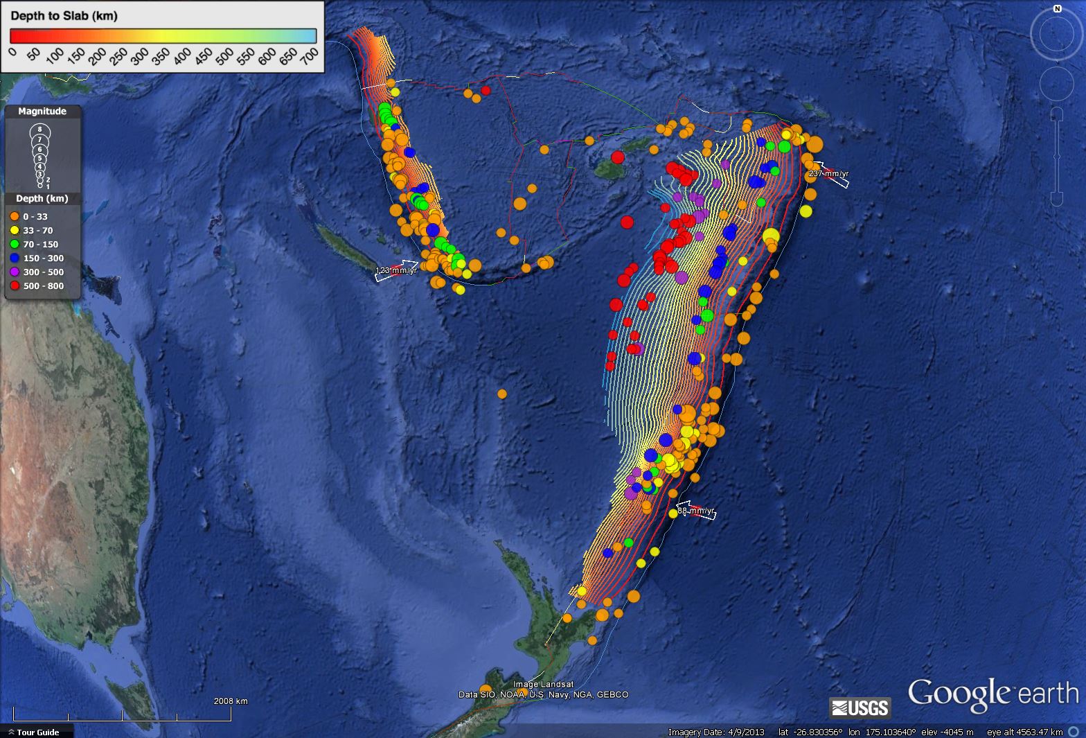
I plot the seismicity from the past month, with color representing depth and diameter representing magnitude (see legend). I include earthquake epicenters from 1918-2018 with magnitudes M ≥ 6.5 in one version.
I plot the USGS fault plane solutions (moment tensors in blue and focal mechanisms in orange), possibly in addition to some relevant historic earthquakes.
- I placed a moment tensor / focal mechanism legend on the poster. There is more material from the USGS web sites about moment tensors and focal mechanisms (the beach ball symbols). Both moment tensors and focal mechanisms are solutions to seismologic data that reveal two possible interpretations for fault orientation and sense of motion. One must use other information, like the regional tectonics, to interpret which of the two possibilities is more likely.
- I also include the shaking intensity contours on the map. These use the Modified Mercalli Intensity Scale (MMI; see the legend on the map). This is based upon a computer model estimate of ground motions, different from the “Did You Feel It?” estimate of ground motions that is actually based on real observations. The MMI is a qualitative measure of shaking intensity. More on the MMI scale can be found here and here. This is based upon a computer model estimate of ground motions, different from the “Did You Feel It?” estimate of ground motions that is actually based on real observations.
- I include the slab 2.0 contours plotted (Hayes, 2018), which are contours that represent the depth to the subduction zone fault. These are mostly based upon seismicity. The depths of the earthquakes have considerable error and do not all occur along the subduction zone faults, so these slab contours are simply the best estimate for the location of the fault.
- In the map below, I include a transparent overlay of the magnetic anomaly data from EMAG2 (Meyer et al., 2017). As oceanic crust is formed, it inherits the magnetic field at the time. At different points through time, the magnetic polarity (north vs. south) flips, the north pole becomes the south pole. These changes in polarity can be seen when measuring the magnetic field above oceanic plates. This is one of the fundamental evidences for plate spreading at oceanic spreading ridges (like the Gorda rise).
- Regions with magnetic fields aligned like today’s magnetic polarity are colored red in the EMAG2 data, while reversed polarity regions are colored blue. Regions of intermediate magnetic field are colored light purple.
Magnetic Anomalies
- In the upper right corner is a plate tectonic map from Ballance et al. (1999) that shows the plate boundary faults in this region of the western Pacific. This shows that the Pacific plate subducts westward beneath the Australia plate. I placed a blue star in the general location of the M 6.9 earthquake (same for other inset figures).
- In the upper left corner is a portion of the map from Benz et al. (2011) that shows earthquake epicenters with color representing depth and diameter representing magnitude. There are several cross sectional data prepared and the location for these cross sections is shown on the map.
- In the lower left corner is cross section J-J’ that shows earthquake hypocenters (3-D locations) in the region of the M 6.9 earthquake.
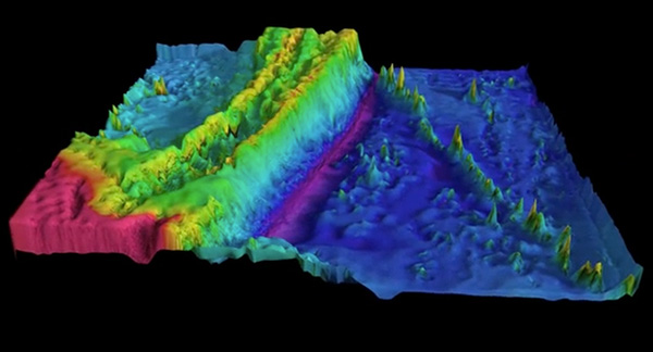
- In the lower right corner, there is a cross section of the Kermadec trench that includes bathymetry of the region (topography of the sea floor). This graphic was created by scientists at Woods Hole. I label the Louisville Seamount Chain for reference to compare with the main map.
I include some inset figures. Some of the same figures are located in different places on the larger scale map below.
- Here is the map with a month’s seismicity plotted.
- Here is the map with a centuries seismicity plotted.
Other Report Pages
Some Relevant Discussion and Figures
- Here is the tectonic map from Ballance et al., 1999.
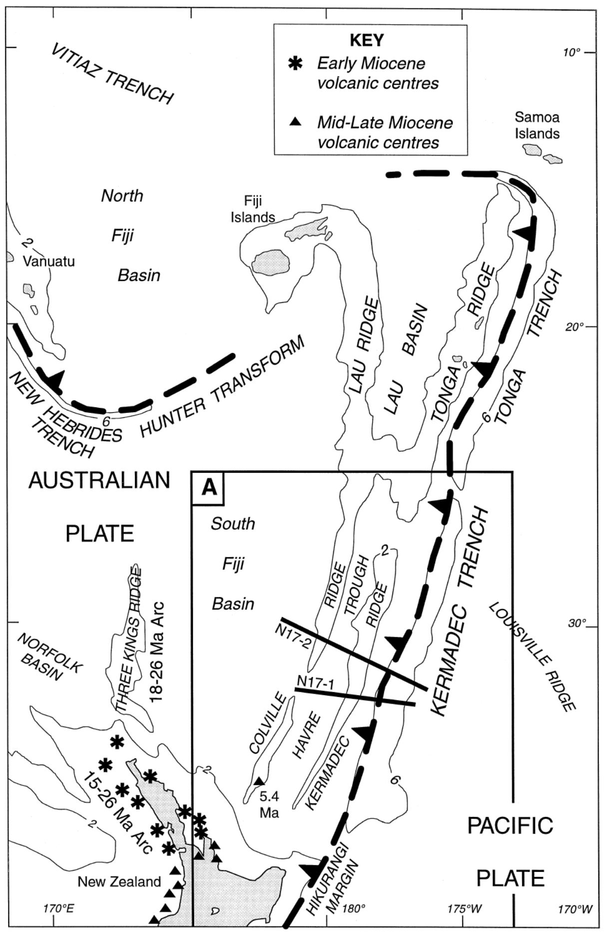
Map of the Southwest Pacific Ocean showing the regional tectonic setting and location of the two dredged profiles. Depth contours in kilometres. The presently active arcs comprise New Zealand–Kermadec Ridge–Tonga Ridge, linked with Vanuatu by transforms associated with the North Fiji Basin. Colville Ridge–Lau Ridge is the remnant arc. Havre Trough–Lau Basin is the active backarc basin. Kermadec–Tonga Trench marks the site of subduction of Pacific lithosphere westward beneath Australian plate lithosphere. North and South Fiji Basins are marginal basins of late Neogene and probable Oligocene age, respectively. 5.4sK–Ar date of dredged basalt sample (Adams et al., 1994).
- Here is a great summary of the fault mechanisms for earthquakes along this plate boundary (Yu, 2013).
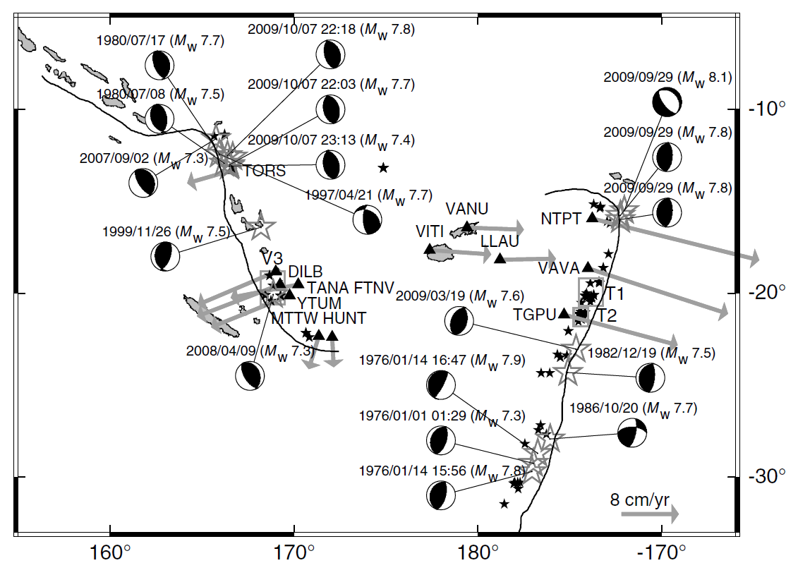
Large subduction-zone interplate earthquakes (large open gray stars) labeled with event date, Mw, GCMT focal mechanisms, and GPS velocity vectors (gray arrows and black triangles labeled with station name). GPS velocities are listed in Table 3. Black lines indicate the Tonga–Kermadec and Vanuatu trenches. Note that the 2009/09/29 Samoa–Tonga outer trench-slope event (Mw 8.1) triggered large interplate doublets (both of Mw 7.8; Lay et al., 2010). The Pacific plate subducts westward beneath the Australian plate along the Tonga–Kermadec trench, whereas the Australian plate subducts eastward beneath the Vanuatu arc and North Fiji basin. The opposite orientation between the Tonga–Kermadec and Vanuatu subduction systems is due to complex and broad back-arc extension in the Lau and North Fiji basins (Pelletier et al., 1998).
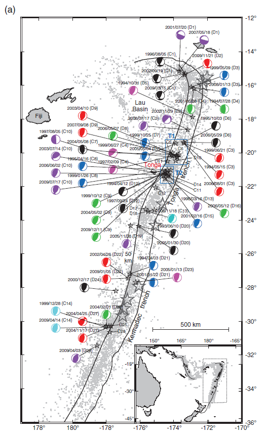
Regional map of moderate-sized (mb > 4:7) shallow-focus repeating earthquakes and background seismicity along the (a) Tonga–Kermadec and (b) Vanuatu (former New Hebrides) subduction zones. Shallow repeating earthquakes (black stars) and their available Global Centroid Moment Tensor (GCMT; Dziewoński et al., 1981; Ekström et al., 2003) are labeled with event date and doublet/cluster id where applicable. Colors of GCMT are used to distinguish nearby different repeaters. Source parameters for the clusters and doublets are listed in Tables 1 and 2. Background seismicity is shown as gray dots and large interplate earthquakes (moment magnitude, Mw > 7:3) since 1976 are shown as large open gray stars. Black lines indicate the trench (Bird, 2003) and slab contour at 50-km depth (Gudmundsson and Sambridge, 1998). Repeating earthquake clusters in the (a) T1 and T2 plate-interface regions in Tonga and (b) V3 plate-interface region in Vanuatu are used to study the fault-slip rate ( _d). A regional map of the Tonga–Kermadec–Vanuatu subduction zones is
shown in the inset figure, with the gray dotted box indicating the expanded region in the main figure.
- Here is a 3-D view of the subducting slab along the Tonga Trench (Green, 2007). While this is to the north of where the M 6.9 happened, it helps us visualize the geometry of the subducting slab. Note how there is a different shape to the slab to the north than to the south. Take a look at the seismicity map in Benz et al., 2011 for comparison.
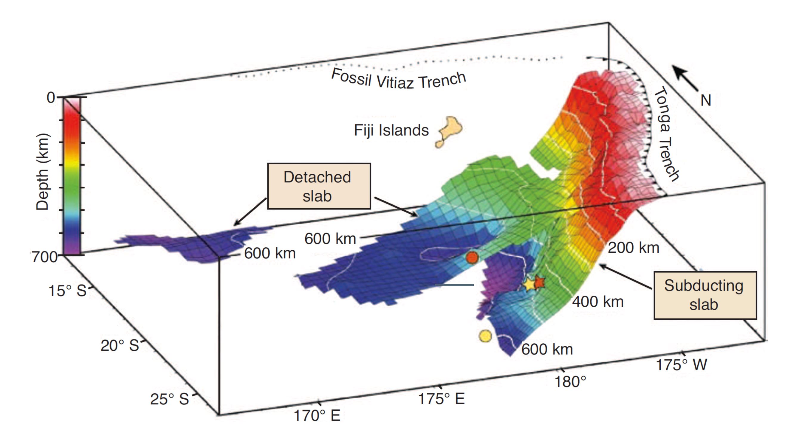
Earthquakes and subducted slabs beneath the Tonga–Fiji area. The subducting slab and detached slab are defined by the historic earthquakes in this region: the steeply dipping surface descending from the Tonga Trench marks the currently active subduction zone, and the surface lying mostly between 500 and 680 km, but rising to 300 km in the east, is a relict from an old subduction zone that descended from the fossil Vitiaz Trench. The locations of the mainshocks of the two Tongan earthquake sequences discussed by Tibi et al.2 are marked in yellow (2002 sequence) and orange (1986 series). Triggering mainshocks are denoted by stars; triggered mainshocks by circles. The 2002 sequence lies wholly in the currently subducting slab (and slightly extends the earthquake distribution in it),whereas the 1986 mainshock is in that slab but the triggered series is located in the detached slab,which apparently contains significant amounts of metastable olive.
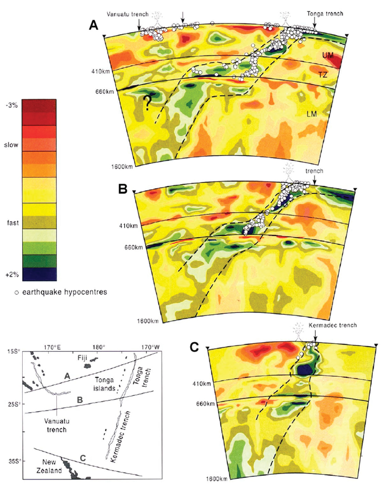
- This is a figure from de Paor et al. (2012) that shows cross sections along the Tonga/Kermadec system. These cross sections are based on “seismic tomographic” methods. Seismic tomography is similar to CT scans, which are “computed tomography” using X-Rays. Seismic tomography uses seismic waves to interrogate Earth’s interior and are calculated using the same general concepts that are used to resolve differences in density using CT scans (“cat scans”). The colors represent the relative seismic velocity of different parts of the lithosphere. Cool colors represent higher velocities, which are found in cold slabs (compared to warmer mantle, where seismic velocities are slower). These authors use the faster velocities to locate the subducting slab. The M 6.9 earthquake happened between cross sections B and C, but the geometry in that area looks more similar to cross section C.
- This is a schematic illustration showing the interpretation from Chang et al. (2015) of the geometry of these subducting slabs. Compare with the Green (2007) figure above.
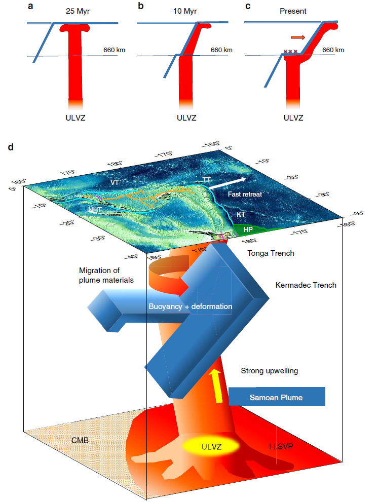
A schematic diagram illustrating the slab–plume interaction beneath the Tonga–Kermadec arc. Cyan lines on the surface show trenches, as shown in Fig. 1. HP, Hikurangi Plateau; KT, Kermadec Trench; NHT, New Hebrides Trench; TT, Tonga Trench; VT, Vitiaz Trench. The Samoan plume originates from a Mega ULVZ at the core–mantle boundary (CMB). The buoyancy caused by large stress from the plume at the bottom of the Tonga slab may contribute to the slab stagnation within the mantle transition zone, while the Kermadec slab is penetrating into the lower mantle directly. At the northern end of the Tonga slab, plume materials migrate into the mantle wedge, facilitated by strong toroidal flow around the slab edge induced by fast slab retreat
- Here is a fantastic summary of the plate boundary in this region (Bird, 2003). There are so many earthquakes here that their symbols overlap each other.

Boundaries (heavy colored lines) of the New Hebrides (NH), Balmoral Reef (BR), Conway Reef (CR), and Futuna (FT) plates. All are included in the New Hebrides-Fiji orogen because of evidence that they may be deforming rapidly. Surrounding plates are Australia (AU), Tonga (TO), Niuafo’ou (NI), and Pacific (PA). Conventions as in Figure 2, except coastlines are blue. Oblique Mercator projection on great circle passing E-W through (17°S, 174°E).
- Here is another map of the bathymetry in this region of the Kermadec trench. This was produced by Jack Cook at the Woods Hole Oceanographic Institution. The Lousiville Seamount Chain is clearly visible in this graphic.
- I put together an animation of seismicity from 1965 – 2015 Sept. 7. Here is a map that shows the entire seismicity for this period. I plot the slab contours for the subduction zone here. These were created by the USGS (Hayes et al., 2012).
- Here is the animation. Download the mp4 file here. This animation includes earthquakes with magnitudes greater than M 6.5 and this is the kml file that I used to make this animation.
- Finally, I would like to show a figure prepared by Dr. Gavin Hayes (USGS) that shows the relations between the two ultra deep earthquakes near Fiji. I did not prepare a report for the M 7.9 earthquake on 2018.09.06, which is the main reason I included this information in this report. Dr. Hayes shows earthquake fault mechanisms (viewed from their side) relative to depth (along with earthquake hypocenters for smaller magnitude earthquakes). The geometry for the downgoing slab is shown as a purple dashed-dotted line. More can be found about this M 7.9 earthquake here.

Geologic Fundamentals
- For more on the graphical representation of moment tensors and focal mechnisms, check this IRIS video out:
- Here is a fantastic infographic from Frisch et al. (2011). This figure shows some examples of earthquakes in different plate tectonic settings, and what their fault plane solutions are. There is a cross section showing these focal mechanisms for a thrust or reverse earthquake. The upper right corner includes my favorite figure of all time. This shows the first motion (up or down) for each of the four quadrants. This figure also shows how the amplitude of the seismic waves are greatest (generally) in the middle of the quadrant and decrease to zero at the nodal planes (the boundary of each quadrant).

- Here is another way to look at these beach balls.
The two beach balls show the stike-slip fault motions for the M6.4 (left) and M6.0 (right) earthquakes. Helena Buurman's primer on reading those symbols is here. pic.twitter.com/aWrrb8I9tj
— AK Earthquake Center (@AKearthquake) August 15, 2018
- There are three types of earthquakes, strike-slip, compressional (reverse or thrust, depending upon the dip of the fault), and extensional (normal). Here is are some animations of these three types of earthquake faults. The following three animations are from IRIS.
Strike Slip:
Compressional:
Extensional:
- This is an image from the USGS that shows how, when an oceanic plate moves over a hotspot, the volcanoes formed over the hotspot form a series of volcanoes that increase in age in the direction of plate motion. The presumption is that the hotspot is stable and stays in one location. Torsvik et al. (2017) use various methods to evaluate why this is a false presumption for the Hawaii Hotspot.
- Here is a map from Torsvik et al. (2017) that shows the age of volcanic rocks at different locations along the Hawaii-Emperor Seamount Chain.

A cutaway view along the Hawaiian island chain showing the inferred mantle plume that has fed the Hawaiian hot spot on the overriding Pacific Plate. The geologic ages of the oldest volcano on each island (Ma = millions of years ago) are progressively older to the northwest, consistent with the hot spot model for the origin of the Hawaiian Ridge-Emperor Seamount Chain. (Modified from image of Joel E. Robinson, USGS, in “This Dynamic Planet” map of Simkin and others, 2006.)

Hawaiian-Emperor Chain. White dots are the locations of radiometrically dated seamounts, atolls and islands, based on compilations of Doubrovine et al. and O’Connor et al. Features encircled with larger white circles are discussed in the text and Fig. 2. Marine gravity anomaly map is from Sandwell and Smith.
- 2018.09.09 M 6.9 Kermadec
- 2018.08.29 M 7.1 Loyalty Islands
- 2018.08.18 M 8.2 Fiji
- 2018.03.26 M 6.9 New Britain
- 2018.03.26 M 6.6 New Britain
- 2018.03.08 M 6.8 New Ireland
- 2018.02.25 M 7.5 Papua New Guinea
- 2018.02.26 M 7.5 Papua New Guinea Update #1
- 2017.11.19 M 7.0 Loyalty Islands Update #1
- 2017.11.07 M 6.5 Papua New Guinea
- 2017.11.04 M 6.8 Tonga
- 2017.10.31 M 6.8 Loyalty Islands
- 2017.08.27 M 6.4 N. Bismarck plate
- 2017.05.09 M 6.8 Vanuatu
- 2017.03.19 M 6.0 Solomon Islands
- 2017.03.05 M 6.5 New Britain
- 2017.01.22 M 7.9 Bougainville
- 2017.01.03 M 6.9 Fiji
- 2016.12.17 M 7.9 Bougainville
- 2016.12.08 M 7.8 Solomons
- 2016.10.17 M 6.9 New Britain
- 2016.10.15 M 6.4 South Bismarck Sea
- 2016.09.14 M 6.0 Solomon Islands
- 2016.08.31 M 6.7 New Britain
- 2016.08.12 M 7.2 New Hebrides Update #2
- 2016.08.12 M 7.2 New Hebrides Update #1
- 2016.08.12 M 7.2 New Hebrides
- 2016.04.06 M 6.9 Vanuatu Update #1
- 2016.04.03 M 6.9 Vanuatu
- 2015.03.30 M 7.5 New Britain (Update #5)
- 2015.03.30 M 7.5 New Britain (Update #4)
- 2015.03.29 M 7.5 New Britain (Update #3)
- 2015.03.29 M 7.5 New Britain (Update #2)
- 2015.03.29 M 7.5 New Britain (Update #1)
- 2015.03.29 M 7.5 New Britain
- 2015.11.18 M 6.8 Solomon Islands
- 2015.05.24 M 6.8, 6.8, 6.9 Santa Cruz Islands
- 2015.05.05 M 7.5 New Britain
New Britain | Solomon | Bougainville | New Hebrides | Tonga | Kermadec Earthquake Reports
Earthquake Reports
Social Media
Focal mechanism from GeoNet regional moment tensor solution with oblique-normal faulting at a depth of 112 km, and stations used to calculate the solution. pic.twitter.com/HksVtcddvF
— John Ristau 🇨🇦 🇳🇿 (@SinistralSeismo) September 10, 2018
Displacement waveforms for a few New Zealand stations and Raoul Is (RIZ) from the 10/09/2018 Mw 7.0 Kermadec earthquake, ~750 km north of NZ. We felt this in Upper Hutt as a noticeable wobble, about 40 km north of WEL. pic.twitter.com/12IRY1TDlr
— John Ristau 🇨🇦 🇳🇿 (@SinistralSeismo) September 10, 2018
Mw=7.0, SOUTH OF KERMADEC ISLANDS (Depth: 111 km), 2018/09/10 04:18:59 UTC – Full details here: https://t.co/Qw2GzqwyUl pic.twitter.com/r9KE8Ye78e
— Earthquakes (@geoscope_ipgp) September 10, 2018
- Ballance, P.F., ablaev, A.G., Pushchin, I.K., Pletnev, S.P., Birylina, M.G., Itaya, T., Follas, H.A., and Gibson, G.W., 1999. Morphology and history of the Kermadec trench–arc–backarc basin–remnant arc system at 30 to 32°S: geophysical profile, microfossil and K–Ar data in Marine Geology, v. 149, p. 35-62.
- Bird, P., 2003. An updated digital model of plate boundaries in Geochemistry, Geophysics, Geosystems, v. 4, doi:10.1029/2001GC000252, 52 p.
- Benz, H.M., Herman, Matthew, Tarr, A.C., Furlong, K.P., Hayes, G.P., Villaseñor, Antonio, Dart, R.L., and Rhea, Susan, 2011. Seismicity of the Earth 1900–2010 eastern margin of the Australia plate: U.S. Geological Survey Open-File Report 2010–1083-I, scale 1:8,000,000.
- Chang, S-J., Ferreira, A.M.G., and Faccenda, M., 2016. Upper- and mid-mantle interaction between the Samoan plume and the Tonga–Kermadec slabs in Nature Communications, v. 7, DOI: 10.1038/ncomms10799
- Green, H.W.II, 2007. Shearing instabilities accompanying high-pressure phase transformations and the mechanics of deep earthquakes in PNAS, v. 104, no. 22, p. 9133-9138, www.pnas.org/cgi/doi/10.1073/pnas.0608045104
- Hayes, G., 2018, Slab2 – A Comprehensive Subduction Zone Geometry Model: U.S. Geological Survey data release, https://doi.org/10.5066/F7PV6JNV.
References:
Return to the Earthquake Reports page.
°
≥
ñ