I don’t always have the time to write a proper Earthquake Report. However, I prepare interpretive posters for these events.
Because of this, I present Earthquake Report Lite. (but it is more than just water, like the adult beverage that claims otherwise). I will try to describe the figures included in the poster, but sometimes I will simply post the poster here.
- M 7.3: https://earthquake.usgs.gov/earthquakes/eventpage/us7000dffl/executive
- M 7.4: https://earthquake.usgs.gov/earthquakes/eventpage/us7000dfk3/executive
- M 8.1: https://earthquake.usgs.gov/earthquakes/eventpage/us7000dflf/executive
- M 6.5: https://earthquake.usgs.gov/earthquakes/eventpage/us7000dfq2/executive
- M 6.5: https://earthquake.usgs.gov/earthquakes/eventpage/us7000eeq4/executive
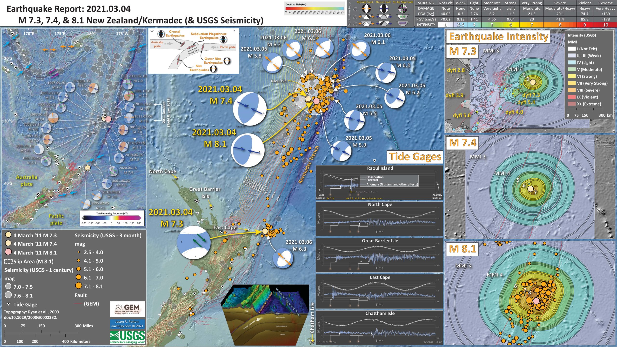
Below is my interpretive poster for this earthquake
- I plot the seismicity from the past month, with diameter representing magnitude (see legend). I include earthquake epicenters from 1921-2021 with magnitudes M ≥ 3.0 in one version.
- I plot the USGS fault plane solutions (moment tensors in blue and focal mechanisms in orange), possibly in addition to some relevant historic earthquakes.
- A review of the basic base map variations and data that I use for the interpretive posters can be found on the Earthquake Reports page. I have improved these posters over time and some of this background information applies to the older posters.
- Some basic fundamentals of earthquake geology and plate tectonics can be found on the Earthquake Plate Tectonic Fundamentals page.
I include some inset figures.
- Here is the map with a month’s seismicity plotted.

UPDATE: 2023.03.04
I added additional context for this event and the regional tectonics.
- In the map above, I include a transparent overlay of the magnetic anomaly data from EMAG2 (Meyer et al., 2017). As oceanic crust is formed, it inherits the magnetic field at the time. At different points through time, the magnetic polarity (north vs. south) flips, the North Pole becomes the South Pole. These changes in polarity can be seen when measuring the magnetic field above oceanic plates. This is one of the fundamental evidences for plate spreading at oceanic spreading ridges (like the Gorda rise).
- Regions with magnetic fields aligned like today’s magnetic polarity are colored red in the EMAG2 data, while reversed polarity regions are colored blue. Regions of intermediate magnetic field are colored light purple.
- We can see the roughly east-west trends of these red and blue stripes. These lines are parallel to the ocean spreading ridges from where they were formed. The stripes disappear at the subduction zone because the oceanic crust with these anomalies is diving deep beneath the Sunda plate (part of Eurasia), so the magnetic anomalies from the overlying Sunda plate mask the evidence for the Australia plate.
Magnetic Anomalies
- In a map above, I include a transparent overlay of the Global Strain Rate Map (Kreemer et al., 2014).
- The mission of the Global Strain Rate Map (GSRM) project is to determine a globally self-consistent strain rate and velocity field model, consistent with geodetic and geologic field observations. The overall mission also includes:
- contributions of global, regional, and local models by individual researchers
- archive existing data sets of geologic, geodetic, and seismic information that can contribute toward a greater understanding of strain phenomena
- archive existing methods for modeling strain rates and strain transients
- The completed global strain rate map will provide a large amount of information that is vital for our understanding of continental dynamics and for the quantification of seismic hazards.
- The version used in the poster(s) below is an update to the original 2004 map (Kreemer et al., 2000, 2003; Holt et al., 2005).
Global Strain
- In the lower right corner is a map that shows the major islands, the major plate tectonic boundaries (the faults, the volcanoes), and the location of two profiles shown above (Ballance et al., 1999. I place a blue star in the general location of the earthquake.
- In the upper right corner are these two profiles (17-1 & 17-2). These profiles show how the elevation changes (solid line) and how the geomagnetic properties intensity, declination, inclination (dashed) vary across the plate boundary.
- In the lower left corner is a map from Benz et al. (2010) that shows earthquakes with circles that represent magnitude (diameter) and depth (color). Deeper = blue & shallower = red. There is a cross section (cut into the earth) profile through this seismicity that uses a source area as shown by a rectangle (the green line J-J’).
- In the upper left corner is cross section J-J’ that shows earthquake hypocenters (3-D locations) in the region of the M 7.2 earthquake.
- there is a cross section of the Kermadec trench that includes bathymetry of the region (topography of the sea floor). This graphic was created by scientists at Woods Hole. I label the Louisville Seamount Chain for reference to compare with the main map.
I include some inset figures. Some of the same figures are located in different places on the larger scale map below.
Some Relevant Discussion and Figures
- Here is the tectonic map from Ballance et al., 1999.
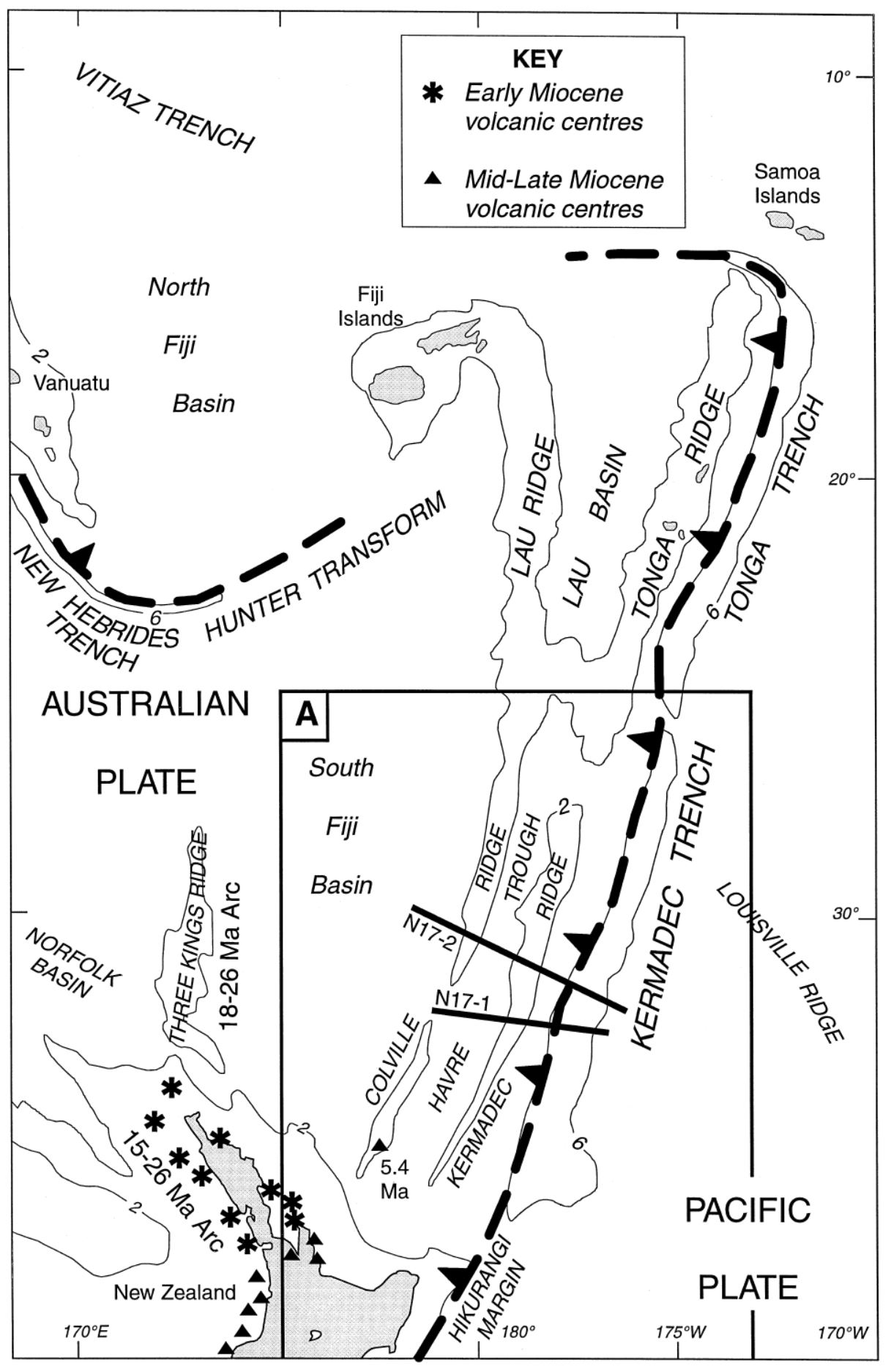
Map of the Southwest Pacific Ocean showing the regional tectonic setting and location of the two dredged profiles. Depth contours in kilometres. The presently active arcs comprise New Zealand–Kermadec Ridge–Tonga Ridge, linked with Vanuatu by transforms associated with the North Fiji Basin. Colville Ridge–Lau Ridge is the remnant arc. Havre Trough–Lau Basin is the active backarc basin. Kermadec–Tonga Trench marks the site of subduction of Pacific lithosphere westward beneath Australian plate lithosphere. North and South Fiji Basins are marginal basins of late Neogene and probable Oligocene age, respectively. 5.4sK–Ar date of dredged basalt sample (Adams et al., 1994).
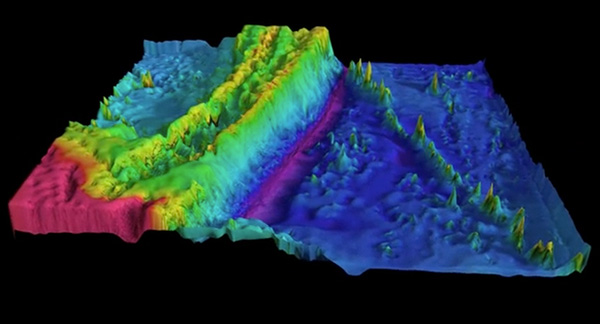
- Here is a great visualization of the Kermadec Trench from Woods Hole.
Kermadec Trench from Woods Hole Oceanographic Inst. on Vimeo.
- Here is another map of the bathymetry in this region of the Kermadec trench. This was produced by Jack Cook at the Woods Hole Oceanographic Institution. The Lousiville Seamount Chain is clearly visible in this graphic.
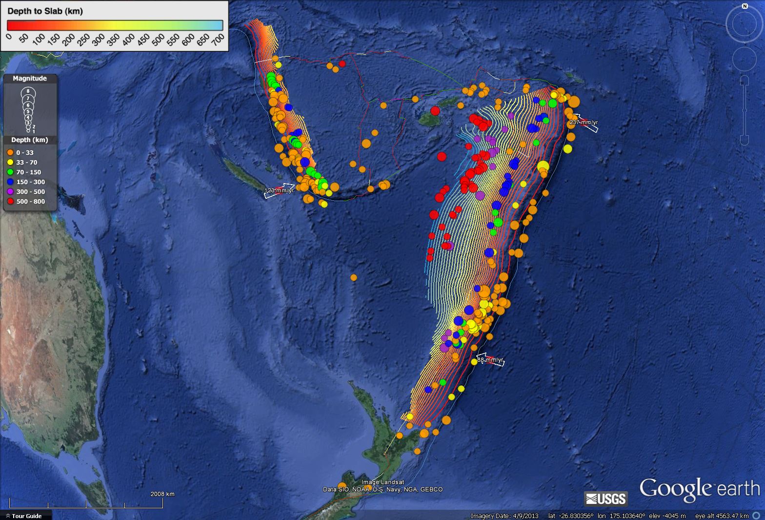
- I put together an animation of seismicity from 1965 – 2015 Sept. 7. Here is a map that shows the entire seismicity for this period. I plot the slab contours for the subduction zone here. These were created by the USGS (Hayes et al., 2012).
- Here is the animation. Download the mp4 file here. This animation includes earthquakes with magnitudes greater than M 6.5 and this is the kml file that I used to make this animation.
Social Media:
If, like me, you're feeling a bit overwhelmed by the wealth of information following yesterday's M7.3, M7.4 & M8.1 earthquakes in the South Pacific, then hopefully this summary map helps, which I've quickly put together. pic.twitter.com/Z6suczfCtT
— Dr Stephen Hicks 🇪🇺 (@seismo_steve) March 5, 2021
- 2021.03.04 M 8.1 Kermadec
- 2019.06.15 M 7.2 Kermadec
- 2019.05.14 M 7.5 New Ireland
- 2019.05.06 M 7.2 Papua New Guinea
- 2018.12.05 M 7.5 New Caledonia
- 2018.10.10 M 7.0 New Britain, PNG
- 2018.09.09 M 6.9 Kermadec
- 2018.08.29 M 7.1 Loyalty Islands
- 2018.08.18 M 8.2 Fiji
- 2018.03.26 M 6.9 New Britain
- 2018.03.26 M 6.6 New Britain
- 2018.03.08 M 6.8 New Ireland
- 2018.02.25 M 7.5 Papua New Guinea
- 2018.02.26 M 7.5 Papua New Guinea Update #1
- 2017.11.19 M 7.0 Loyalty Islands Update #1
- 2017.11.07 M 6.5 Papua New Guinea
- 2017.11.04 M 6.8 Tonga
- 2017.10.31 M 6.8 Loyalty Islands
- 2017.08.27 M 6.4 N. Bismarck plate
- 2017.05.09 M 6.8 Vanuatu
- 2017.03.19 M 6.0 Solomon Islands
- 2017.03.05 M 6.5 New Britain
- 2017.01.22 M 7.9 Bougainville
- 2017.01.03 M 6.9 Fiji
- 2016.12.17 M 7.9 Bougainville
- 2016.12.08 M 7.8 Solomons
- 2016.10.17 M 6.9 New Britain
- 2016.10.15 M 6.4 South Bismarck Sea
- 2016.09.14 M 6.0 Solomon Islands
- 2016.08.31 M 6.7 New Britain
- 2016.08.12 M 7.2 New Hebrides Update #2
- 2016.08.12 M 7.2 New Hebrides Update #1
- 2016.08.12 M 7.2 New Hebrides
- 2016.04.06 M 6.9 Vanuatu Update #1
- 2016.04.03 M 6.9 Vanuatu
- 2015.03.30 M 7.5 New Britain (Update #5)
- 2015.03.30 M 7.5 New Britain (Update #4)
- 2015.03.29 M 7.5 New Britain (Update #3)
- 2015.03.29 M 7.5 New Britain (Update #2)
- 2015.03.29 M 7.5 New Britain (Update #1)
- 2015.03.29 M 7.5 New Britain
- 2015.11.18 M 6.8 Solomon Islands
- 2015.05.24 M 6.8, 6.8, 6.9 Santa Cruz Islands
- 2015.05.05 M 7.5 New Britain
New Britain | Solomon | Bougainville | New Hebrides | Tonga | Kermadec Earthquake Reports
General Overview
Earthquake Reports
- 2016.11.26 M 7.8 New Zealand Post #1
- 2016.12.03 M 7.8 New Zealand Post #2
- 2016.08.18 M 5.7 Australia
- 2016.02.15 M 6.2 Macquarie Island
- 2016.02.14 M 5.8 New Zealand
- 2013.08.15 M 6.8 New Zealand
New Zealand | Australia
General Overview
Earthquake Reports
- Frisch, W., Meschede, M., Blakey, R., 2011. Plate Tectonics, Springer-Verlag, London, 213 pp.
- Hayes, G., 2018, Slab2 – A Comprehensive Subduction Zone Geometry Model: U.S. Geological Survey data release, https://doi.org/10.5066/F7PV6JNV.
- Holt, W. E., C. Kreemer, A. J. Haines, L. Estey, C. Meertens, G. Blewitt, and D. Lavallee (2005), Project helps constrain continental dynamics and seismic hazards, Eos Trans. AGU, 86(41), 383–387, , https://doi.org/10.1029/2005EO410002. /li>
- Jessee, M.A.N., Hamburger, M. W., Allstadt, K., Wald, D. J., Robeson, S. M., Tanyas, H., et al. (2018). A global empirical model for near-real-time assessment of seismically induced landslides. Journal of Geophysical Research: Earth Surface, 123, 1835–1859. https://doi.org/10.1029/2017JF004494
- Kreemer, C., J. Haines, W. Holt, G. Blewitt, and D. Lavallee (2000), On the determination of a global strain rate model, Geophys. J. Int., 52(10), 765–770.
- Kreemer, C., W. E. Holt, and A. J. Haines (2003), An integrated global model of present-day plate motions and plate boundary deformation, Geophys. J. Int., 154(1), 8–34, , https://doi.org/10.1046/j.1365-246X.2003.01917.x.
- Kreemer, C., G. Blewitt, E.C. Klein, 2014. A geodetic plate motion and Global Strain Rate Model in Geochemistry, Geophysics, Geosystems, v. 15, p. 3849-3889, https://doi.org/10.1002/2014GC005407.
- Meyer, B., Saltus, R., Chulliat, a., 2017. EMAG2: Earth Magnetic Anomaly Grid (2-arc-minute resolution) Version 3. National Centers for Environmental Information, NOAA. Model. https://doi.org/10.7289/V5H70CVX
- Müller, R.D., Sdrolias, M., Gaina, C. and Roest, W.R., 2008, Age spreading rates and spreading asymmetry of the world’s ocean crust in Geochemistry, Geophysics, Geosystems, 9, Q04006, https://doi.org/10.1029/2007GC001743
- Pagani,M. , J. Garcia-Pelaez, R. Gee, K. Johnson, V. Poggi, R. Styron, G. Weatherill, M. Simionato, D. Viganò, L. Danciu, D. Monelli (2018). Global Earthquake Model (GEM) Seismic Hazard Map (version 2018.1 – December 2018), DOI: 10.13117/GEM-GLOBAL-SEISMIC-HAZARD-MAP-2018.1
- Silva, V ., D Amo-Oduro, A Calderon, J Dabbeek, V Despotaki, L Martins, A Rao, M Simionato, D Viganò, C Yepes, A Acevedo, N Horspool, H Crowley, K Jaiswal, M Journeay, M Pittore, 2018. Global Earthquake Model (GEM) Seismic Risk Map (version 2018.1). https://doi.org/10.13117/GEM-GLOBAL-SEISMIC-RISK-MAP-2018.1
- Zhu, J., Baise, L. G., Thompson, E. M., 2017, An Updated Geospatial Liquefaction Model for Global Application, Bulletin of the Seismological Society of America, 107, p 1365-1385, https://doi.org/0.1785/0120160198
- Richards, S., Holm, R., and Barber, G., 2011. Skip Nav Destination When slabs collide: A tectonic assessment of deep earthquakes in the Tonga-Vanuatu region in Geology, c. 39, no. 8, p. 787-790, https://doi.org/10.1130/G31937.1
- Timm, C., Bassett, D., Graham, I. et al. Louisville seamount subduction and its implication on mantle flow beneath the central Tonga–Kermadec arc. Nat Commun 4, 1720 (2013). https://doi.org/10.1038/ncomms2702
References:
Basic & General References
Specific References
Return to the Earthquake Reports page.
- Sorted by Magnitude
- Sorted by Year
- Sorted by Day of the Year
- Sorted By Region