This evening (my time) there was an earthquake in Morocco. Magnitude 6.8, rather shallow, reverse or thrust (compressional) mechanism.
https://earthquake.usgs.gov/earthquakes/eventpage/us7000kufc/executive
This M 6.8 earthquake happened in the Atlas Mountains, a compressional system with south dipping reverse faults on the north and north dipping reverse faults on the south.
It is possible, if not probable, that this earthquake is related to one of these reverse faults. Based on the location, it seems possible that this earthquake is on a south dipping thrust fault (associated with the North Atlas fault system).
I used the USGS earthquake catalog and it appears that this is the largest magnitude earthquake to happen in Morocco (since we started recording earthquakes on seismometers).
Here is the sobering part of this earthquake. The USGS PAGER Alert provides an estimate for the number of casualties and economic impact. Read more about how these estimates are produced (and how to read this report) here.
UPDATE: (2023.09.10 Version 7)
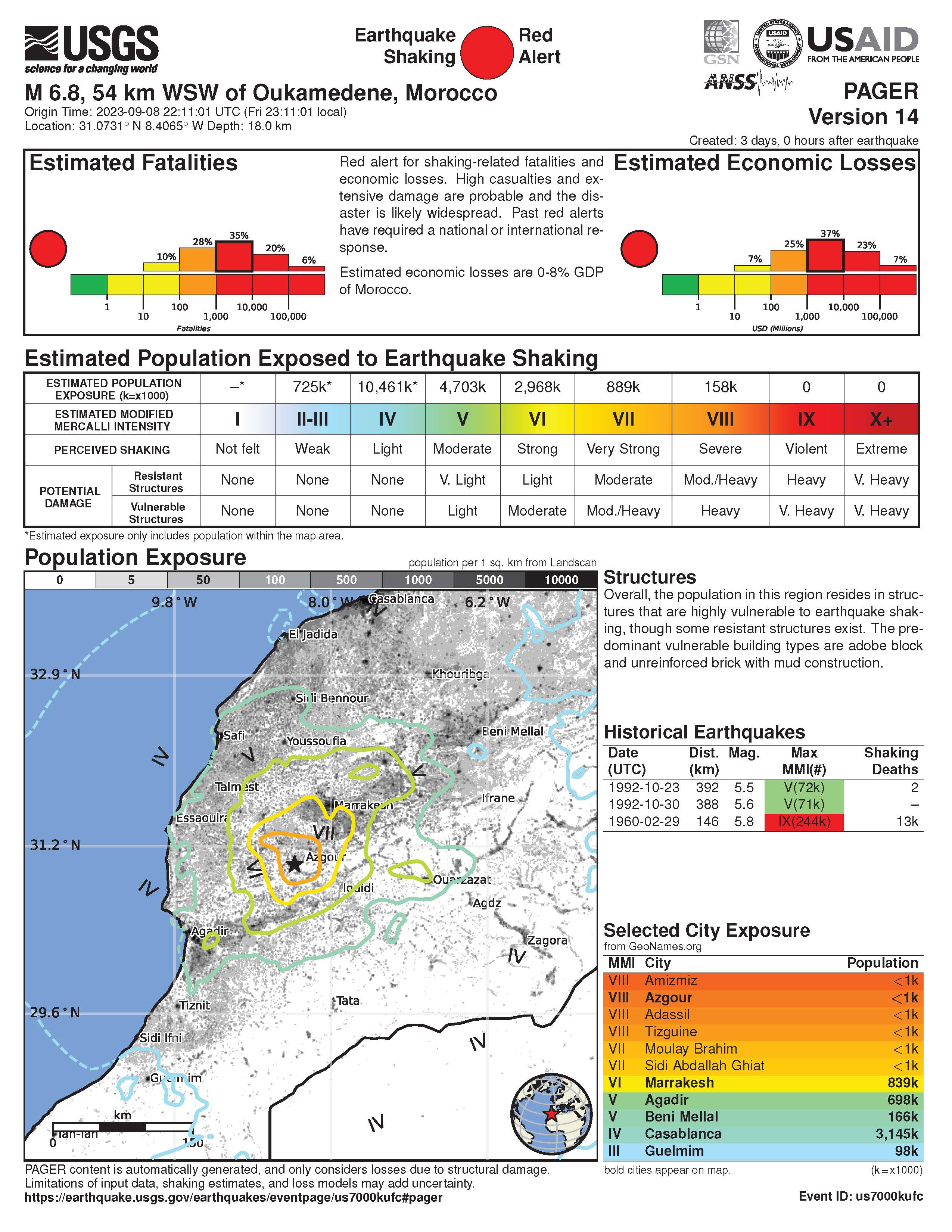
UPDATE: (2023.09.11)
Fault Scaling Relations
Empirical fault scaling relations are ways that we can compare fault rupture sizes with earthquake magnitudes. One of the most used and well cited empirical fault scaling relations paper is Wells and Coppersmith, 1994.
- Wells and Coppersmith developed relations between earthquake magnitude/moment magnitude and surface rupture length, subsurface rupture length, and rupture area. They also consider the difference between mean and maximum displacement measures.
- The length of fault rupture is the distance that the fault slipped measured parallel to Earth’s surface. When we see fault lines mapped on a map, these lines are representative of the fault length.
- The width of fault rupture is the distance that the fault slipped measured down into the Earth. For a fault that dips straight down into the Earth (perpendicular to the Earth’s surface), the width of the fault rupture is the distance between the Earth’s surface and the depth where the fault slipped. For faults that dip at an angle (like along a subduction zone, or a reverse/thrust fault like the fault that caused this M 6.8 earthquake), the distance measured is measured along this non-perpendicular distance.
- The area of fault slip is basically the fault length times the fault width.
- There have been some updates to these scaling relations that attempt to improve these relations. However, Wells and Coppersmith still work pretty well (the updates are not really that much different).
- There remain certain types of earthquakes where we have small amounts of information to constrain these relations for those types of earthquakes (particularly large magnitude earthquakes, which are more rare than small and medium sized earthquakes). So, there is room for improvement.
- Note that there is lots of variation, so these empirical relations (represented by the lines that are drawn to “fit” these data) have lots of range. So, these empirical relations are not perfect predictors (i.e., fault length does not perfectly predict magnitude).
- For example, a fault with subsurface rupture length of 10 km could have a magnitude that ranges between 5.25 and 6.25+. Remember, a M 6.25 releases about 32 times as much energy as a M 5.25. A M 6.25 earthquake is much larger than a M 5.25.
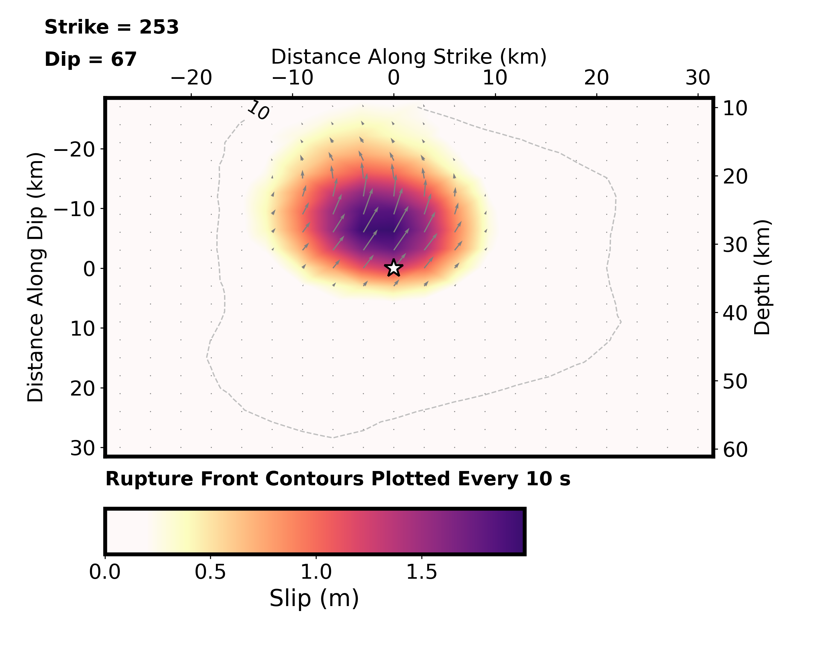
- The M 6.8 USGS earthquake slip model suggests that this earthquake fits well with these subsurface fault scaling relations from Wells and Coppersmith (1994).
- Well, as I was wrapping up for the day, I refreshed the USGS website for the earthquake and they had updated a bunch of the data (intensity, GIS data, and the slip data). So, the slip model shows a much smaller slip area. Though, if we look at the EMSC aftershock region, we may think that their first slip model was better. The aftershock region has a better fit for the scaling relations.
Here is the USGS fault slip model for the M 6.8 earthquake. The length of the fault slip figure is about 40 kilometers (km) and the width of the fault is about 45 km. The color represents the amount that the fault slipped (in meters) during the earthquake. So, the slip area does not fill this entire area. Most of the slip length is within ~30 km and width is within ~35km. The maximum slip is ~1.7 meters.
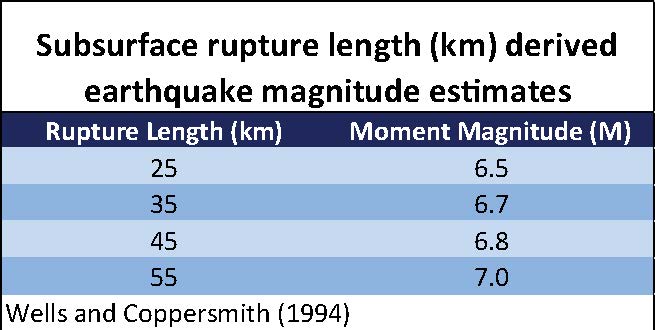
Here is a plot from Wells and Coppersmith that shows the data relating magnitude with subsurface rupture length. We can see that there is a positive relation between magnitude and length (as the length is larger, so is the magnitude).
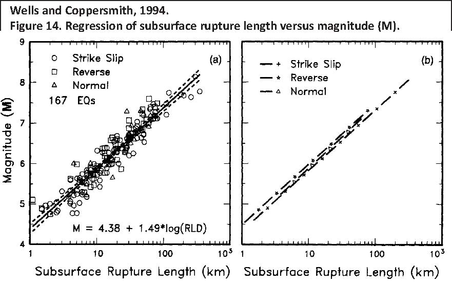
(a) Regression of subsurface rupture length on magnitude (M). Regression line shown for all-slip-type relationship. Short dashed line indicates 95% confidence interval. (b) Regression lines for strike-slip relationships. See
Table 2 for regression coefficients. Length of regression lines shows the range of data for each relation.
So, I used these scaling relations to calculate the magnitude for earthquakes of varying subsurface fault length. Here is a table from those calculations.
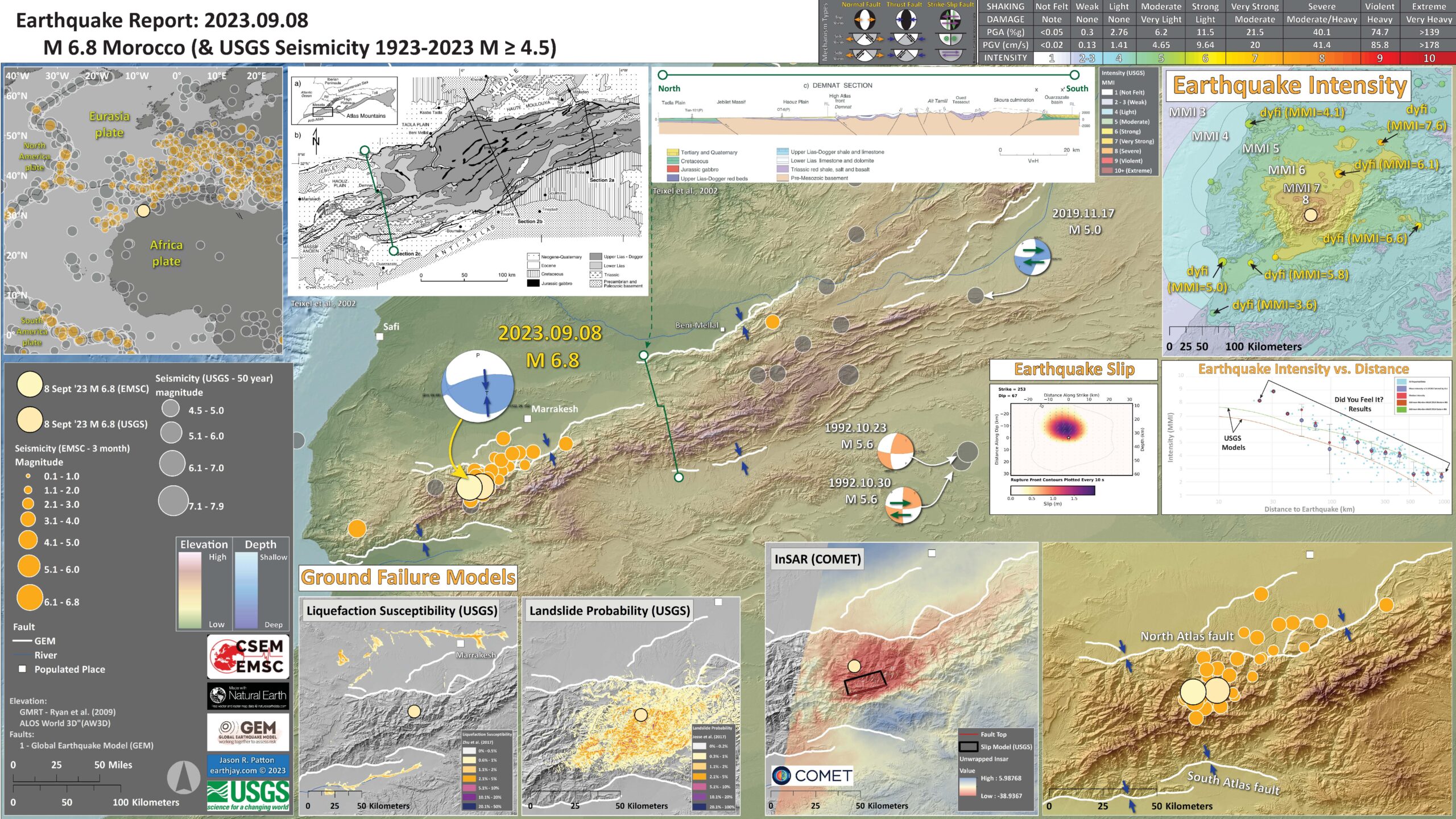
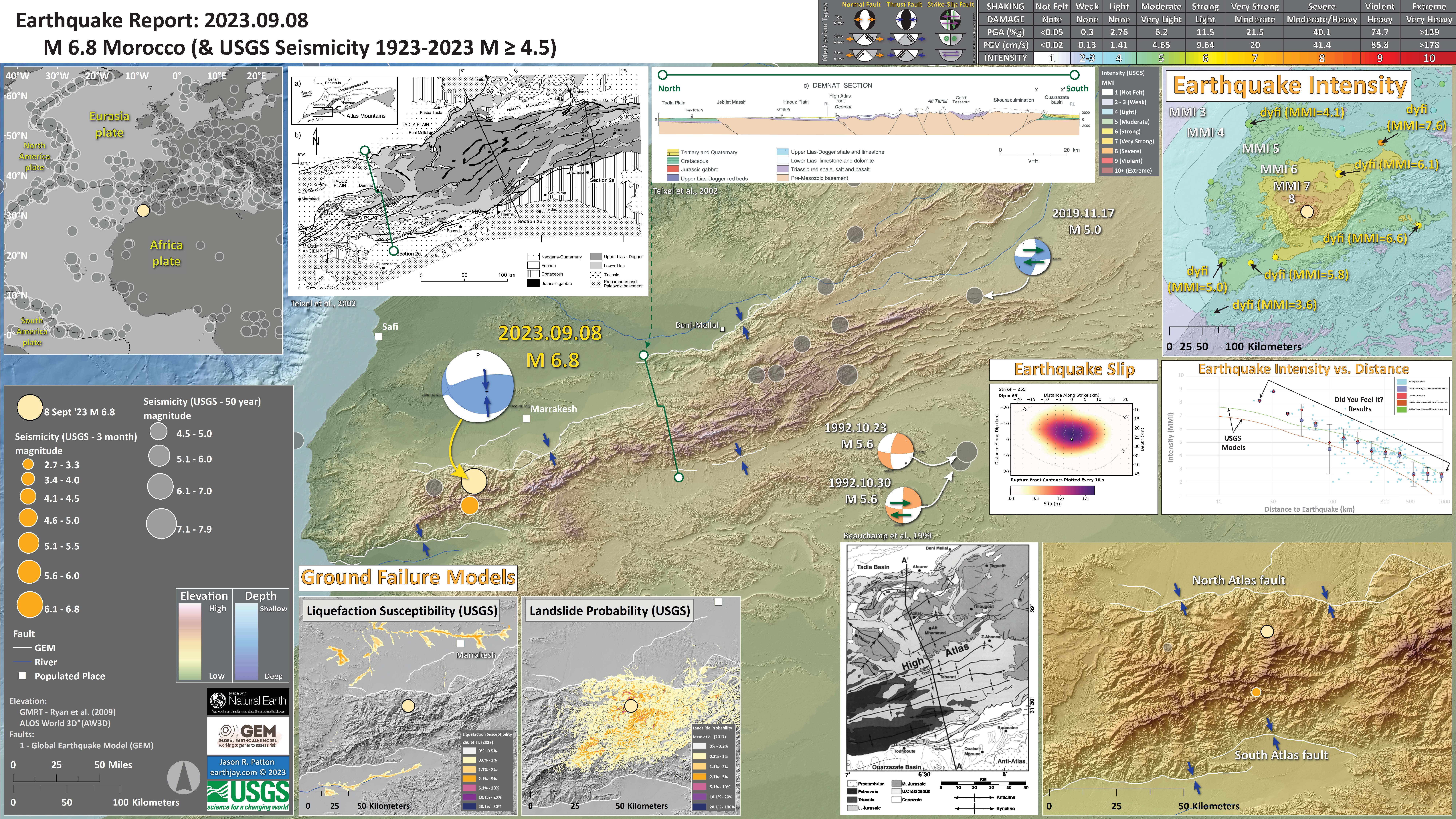
Below is my interpretive poster for this earthquake
- I plot the seismicity from the past month, with diameter representing magnitude (see legend). I include earthquake epicenters from 1922-2022 with magnitudes M ≥ 3.0 in one version.
- I plot the USGS fault plane solutions (moment tensors in blue and focal mechanisms in orange), possibly in addition to some relevant historic earthquakes.
- A review of the basic base map variations and data that I use for the interpretive posters can be found on the Earthquake Reports page. I have improved these posters over time and some of this background information applies to the older posters.
- Some basic fundamentals of earthquake geology and plate tectonics can be found on the Earthquake Plate Tectonic Fundamentals page.
- In the upper left corner is a map that shows the tectonic plates and seismicity for northwestern Africa.
- In the upper right corner is a map that shows the earthquake intensity using the modified Mercalli intensity scale. Earthquake intensity is a measure of how strongly the Earth shakes during an earthquake, so gets smaller the further away one is from the earthquake epicenter. The map colors represent a model of what the intensity may be.
- Below the intensity map is a plot that shows the same intensity (both modeled and reported) data as displayed on the map. Note how the intensity gets smaller with distance from the earthquake.
- In the lower left center are two maps showing the probability of earthquake triggered landslides and possibility of earthquake induced liquefaction. I will describe these phenomena below.
- In the lower right corner is a larger scale map showing the Atlas Mountains and the North and South Atlas faults.
- To the left of this large scale map is a map from Beauchamp et al., 1999. This map is for the Atlas Mtns to the east of where this earthquake happened. Note the tectonic folds associated with the underlying reverse faults.
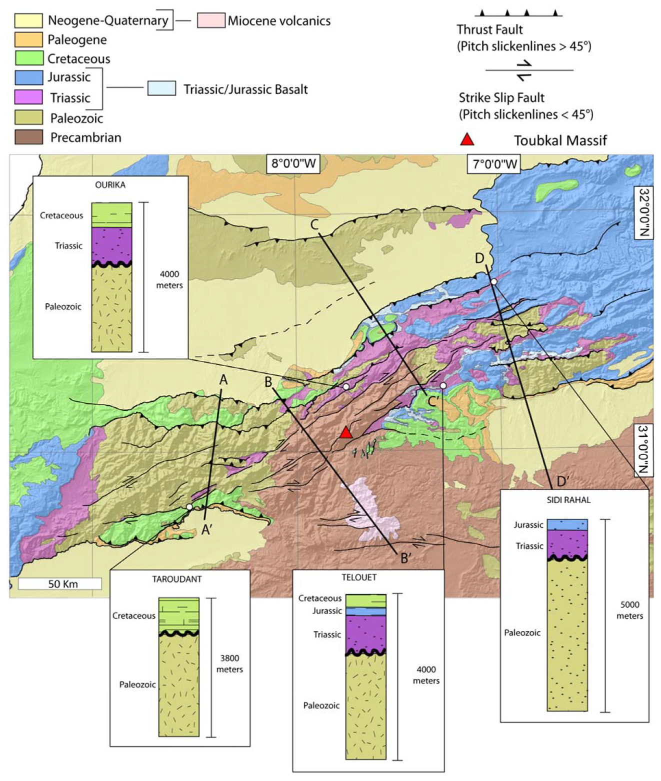
- In the upper left is a map from TEixel et al. (1999) that includes cross section locations. Cross section C is displayed to the right. The location of this cross section is also shown on the main map with the green line.
- To the left of the intensity map is a map from Banault et al. (2023) that includes a yellow star where the M 6.8 earthquake occurred.
I include some inset figures. Some of the same figures are located in different places on the larger scale map below.
- Here is the map with a month’s seismicity plotted.
- This is an updated poster with COMET InSAR analytical results. I also figured out how to download the EMSC seismicity data (they changed their website, so had to learn something new. Here is where one may download data from their catalog.
- The USGS earthquake catalog (aka ComCat) is a global network, so a global catalog. The EMSC catalog relies, in places, on a more local network, so has more events in the catalog than in ComCat.
- However, ComCat usually has all the major events and spans a longer time period.
- SO, the 3 month seismicity I use here is from EMSC and the century dataset is based on the ComCat catalog.
Other Report Pages
- INGV: https://ingvterremoti.com/2023/09/12/terremoto-in-marocco-aggiornamento-del-12-settembre-2023/
- INGV: http://terremoti.ingv.it/en/finitesource_summary/36092321#SorgenteEstesa
- Dr. Judith Hubbard: https://earthquakeinsights.substack.com/p/deadly-m68-earthquake-hits-morocco
- Dr. Judith Hubbard re: InSar Explanation https://earthquakeinsights.substack.com/p/satellite-images-suggest-slip-on
- USGS: https://earthquake.usgs.gov/earthquakes/eventpage/us7000kufc/region-info
- EERI: https://www.eeri.org/about-eeri/news/18451-eeri-response-to-september-8-2023-m6-8-morocco-earthquake
- tEMBLOR: https://temblor.net/temblor/2023-morocco-quake-africa-europe-collision-15527/
Discussion about aftershocks
-
the following is a series of statements that i wrote to respond to someone who is in Morocco. i thought that perhaps others might find this useful.
aftershocks may last for weeks, possibly months. aftershocks typically decay at a rate that is dependent on the fault system. each fault system is slightly different.
Here is a short story about aftershocks in Northern California but this story is relevant to earthquakes elsewhere.
we don’t know the specific rate of decay for a fault system until we observe the aftershocks decay for that fault. some faults have few aftershocks and others have robust aftershock sequences (many events).
it is not satisfying to not know how long they will last, i understand.
e.g., there was an earthquake in central Washington USA in 1872 and some argue that this continues to have aftershocks.
so, they will last a while and nobody will know when they will stop.
but for people to feel safe to start living in their homes again, they need to get an expert, like an engineer, to evaluate the stability of their houses. only an expert, who is trained to inspect structures, can make these evaluations.
will there be other large earthquakes? this is something nobody can know.
follow advice for getting an engineer to check out one’s building(s) so that they can feel safe living in them; if the engineer decides that the structure is safe to withstand earthquakes, that is the best we can do.
the M6.8 changed the stresses in the crust adjacent to the earthquake. in some places, these stresses increased the chance for earthquakes on different (or the same) faults. in other places, they decreased the stress.
these changes in stress are modest but can trigger a new earthquake. but this depends on the state of stress of the other earthquake fault, something that we cannot yet know. so, we cannot know if the places where stress is increased will have a triggered/new earthquake.
the best we can do is to make sure that buildings are resistant to earthquake forces. this capability is reliant on engineers, building inspectors, competent building contractors, building codes, etc. AND that these people follow the rules (building codes).
the Feb 2023 Türkiye earthquakes destroyed buildings that were constructed under well designed building codes. but they were destroyed because people did not follow the code. lots of buildings were built before the codes existed and those did not perform well either.
so, when living in earthquake country, one simply needs to ensure that they are living/working in earthquake resistant buildings. they may find comfort to live outside these structures until they are inspected. this is the smart thing to do.
i don’t have the expertise to know if a building is designed to withstand earthquakes. i am not a structural engineer, an earthquake engineer. i know some and can follow the local building codes here where i live. and i sure could not offer advice remotely. one simply needs to seek local expertise. i wish i could offer more advice.
finally, people who have been traumatized by this earthquake and continue to be traumatized by these aftershocks are going through what everyone does when faced with these conditions. this is typical. maybe finding comfort with friends and family and neighbors will help (?).
i hope i have provided some constructive feedback to your questions/concerns.
hopefully this information can help those in Morocco cope with this extremely challenging natural hazard.
if nothing else, the survivors will be able to build back stronger and more earthquake resistant.
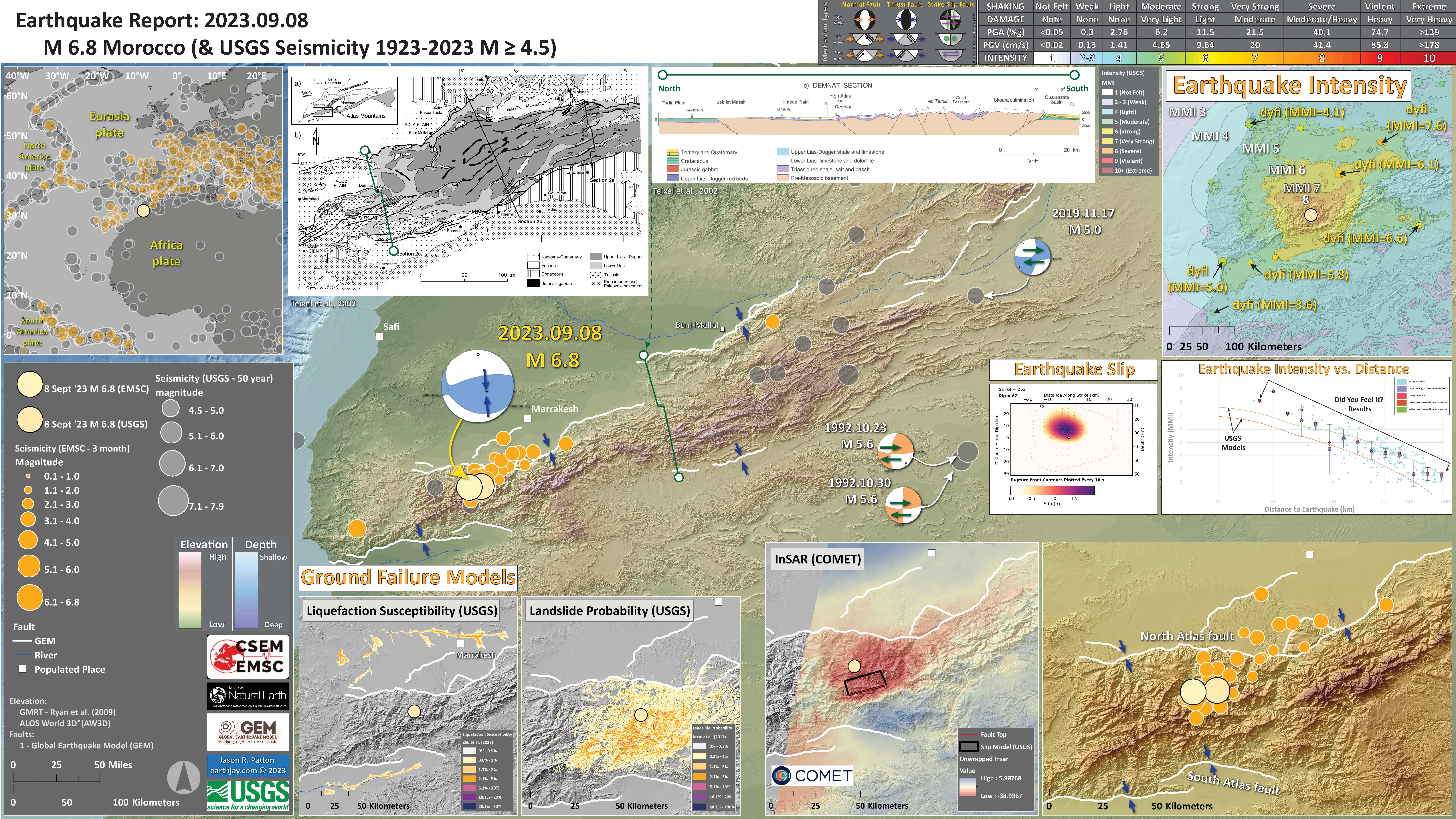
Shaking Intensity
- Here is a figure that shows a more detailed comparison between the modeled intensity and the reported intensity. Both data use the same color scale, the Modified Mercalli Intensity Scale (MMI). More about this can be found here. The colors and contours on the map are results from the USGS modeled intensity. The DYFI data are plotted as colored dots (color = MMI, diameter = number of reports).
- In the upper panel is the USGS Did You Feel It reports map, showing reports as colored dots using the MMI color scale. Underlain on this map are colored areas showing the USGS modeled estimate for shaking intensity (MMI scale).
- In the lower panel is a plot showing MMI intensity (vertical axis) relative to distance from the earthquake (horizontal axis). The models are represented by the green and orange lines. The DYFI data are plotted as light blue dots. The mean and median (different types of “average”) are plotted as orange and purple dots. Note how well the reports fit the green line (the model that represents how MMI works based on quakes in California).
- Below the lower plot is the USGS MMI Intensity scale, which lists the level of damage for each level of intensity, along with approximate measures of how strongly the ground shakes at these intensities, showing levels in acceleration (Peak Ground Acceleration, PGA) and velocity (Peak Ground Velocity, PGV).
Potential for Ground Failure
- Below are a series of maps that show the potential for landslides and liquefaction. These are all USGS data products.
There are many different ways in which a landslide can be triggered. The first order relations behind slope failure (landslides) is that the “resisting” forces that are preventing slope failure (e.g. the strength of the bedrock or soil) are overcome by the “driving” forces that are pushing this land downwards (e.g. gravity). The ratio of resisting forces to driving forces is called the Factor of Safety (FOS). We can write this ratio like this:FOS = Resisting Force / Driving Force
- When FOS > 1, the slope is stable and when FOS < 1, the slope fails and we get a landslide. The illustration below shows these relations. Note how the slope angle α can take part in this ratio (the steeper the slope, the greater impact of the mass of the slope can contribute to driving forces). The real world is more complicated than the simplified illustration below.
- Landslide ground shaking can change the Factor of Safety in several ways that might increase the driving force or decrease the resisting force. Keefer (1984) studied a global data set of earthquake triggered landslides and found that larger earthquakes trigger larger and more numerous landslides across a larger area than do smaller earthquakes. Earthquakes can cause landslides because the seismic waves can cause the driving force to increase (the earthquake motions can “push” the land downwards), leading to a landslide. In addition, ground shaking can change the strength of these earth materials (a form of resisting force) with a process called liquefaction.
- Sediment or soil strength is based upon the ability for sediment particles to push against each other without moving. This is a combination of friction and the forces exerted between these particles. This is loosely what we call the “angle of internal friction.” Liquefaction is a process by which pore pressure increases cause water to push out against the sediment particles so that they are no longer touching.
- An analogy that some may be familiar with relates to a visit to the beach. When one is walking on the wet sand near the shoreline, the sand may hold the weight of our body generally pretty well. However, if we stop and vibrate our feet back and forth, this causes pore pressure to increase and we sink into the sand as the sand liquefies. Or, at least our feet sink into the sand.
- Below is a diagram showing how an increase in pore pressure can push against the sediment particles so that they are not touching any more. This allows the particles to move around and this is why our feet sink in the sand in the analogy above. This is also what changes the strength of earth materials such that a landslide can be triggered.
- Below is a diagram based upon a publication designed to educate the public about landslides and the processes that trigger them (USGS, 2004). Additional background information about landslide types can be found in Highland et al. (2008). There was a variety of landslide types that can be observed surrounding the earthquake region. So, this illustration can help people when they observing the landscape response to the earthquake whether they are using aerial imagery, photos in newspaper or website articles, or videos on social media. Will you be able to locate a landslide scarp or the toe of a landslide? This figure shows a rotational landslide, one where the land rotates along a curvilinear failure surface.
- Below is the liquefaction susceptibility and landslide probability map (Jessee et al., 2017; Zhu et al., 2017). Please head over to that report for more information about the USGS Ground Failure products (landslides and liquefaction). Basically, earthquakes shake the ground and this ground shaking can cause landslides.
- I use the same color scheme that the USGS uses on their website. Note how the areas that are more likely to have experienced earthquake induced liquefaction are in the valleys. Learn more about how the USGS prepares these model results here.


Remote Sensing of Surface Deformation
- One way to learn about the processes that happen during an earthquake is to evaluate the “coseismic” (during earthquake) surface deformation from that earthquake.
- There are many ways to do this type of analysis. One may use classic surveys (using levels and tape measures) to measure the changes. One may use digital observations from satellites or airplanes, called remote sensing.
- One of the ways to do this remote sensing is with a method called interferometric synthetic aperture radar (InSAR).
- The techniques to apply InSAR methods are advanced and take years to master. I will not attempt to explain the full description of what InSAR is but below is a list of online resources where others do a great job at explaining InSAR:
- Basically, there are satellites that pass over Earth over a regular schedule. These satellites have sensors (called platforms) that acquire a variety of data that span different parts of the electromagnetic spectrum.
- Many are familiar with the visible light part of the electromagnetic spectrum (recall the Pink Floyd album, The Dark Side of the Moon, which has an image of light going through a prism, showing the different colors of the visible spectrum.
- The different parts of the electromagnetic spectrum are described by the wavelength of the waves that these different types of radiation use to travel. The wavelength span for blue light is between 400 and 500 nanometers (nm). Green is 500 to 600 nm and red is 600 to 700 nm.
- Other bands have longer or shorter wavelengths. X-Rays have much shorter wavelengths and infrared radiation has longer wavelengths.
- Radar operates at long wavelengths (1-100 cm or 10,000,000-1,000,000,000 nm)
- InSAR analysis, generally, uses radar data collected at two different times to determine how the Earth’s surface moved between the radar acquisitions.
- There are some organizations that have programs that staff people to work on these InSAR analyses for events like earthquakes. NASA Jet Propulsion Laboratory (JPL) and the Centre for Observation and Modeling of Earthquakes, Volcanoes, and Tectonics (COMET) are two of these programs. They provide the results from their analyses online for anyone to download for free.
- Here is the COMET event page for this M6.8 Morocco Earthquake.
- This is a plot of the “unwrapped” InSAR results from the first Sentinel 1 (one of the radar satellites used for InSAR analysis) post-earthquake radar acquisition.
- Color represents how the surface moved towards or away from the Satellite between 30 August and 11 September 2023. This is an ascending track and once we get a descending track acquisition, we will be able to get a better idea of the coseismic deformation.
- This result helps us learn that the area in red generally went up and that the fault is dipping to the north (looking at the unwrapped data in the lower panel help with this interpretation).
- Here is the source of data that I used to plot the above figures.
Learning Resource: Sentinel-1 Synthetic Aperture Radar Interferometric Coherence Image Services StoryMap
This StoryMap tutorial enhances access to the Global Seasonal Sentinel-1 Interferometric Coherence and Backscatter dataset with image services. #SAR https://t.co/VjghtQiBUL pic.twitter.com/zMNLwuAdi3
— NASAEarthdata (@NASAEarthData) September 11, 2023
- Here is the tectonic map from the poster (Teizel et al., 2002).
- Here is the cross section from the poster (Teizel et al., 2002).
- This part of the world was once a mid ocean spreading ridge (aka a rifted margin). This figure shows the tectonic plate boundary configurations from this time of Earth’s past.
- We will revisit this paper further down in the report where we see a geologic map and cross section in the region of this M 6.8 earthquake.
- Here is the Babault et al. (2013) tectonic map.
- Here are the Babault et al. (2013) cross sections.
- The following are some maps from Lanari et al. (2020).
- This is the main tectonic map.
- This is a map that shows how complicated the faulting is in this region.
- Here is a study about the geodetics of the western Mediterranean (Vernant et al., 2010). This study just barely reaches into the western Atlas Mountains, where the M 6.8 earthquake happened.
- Geodesy is the study of the deformation of the Earth’s surface. Geodesists may study interseismic (between earthquakes) deformation or coseismic (during earthquakes) deformation.
- These researchers used Global Positioning System (GPS, like in your smartphone) to measure the motion of locations in this area of study.
- This map shows the two profiles plotted in the next figure. Profile 1 is of interest.
- Profile 1 makes it into the western Atlas Mountains.
- On the left, note sites MARO and AZIL. Look at the profile normal plot (the vertical axis represents how much the sites are moving relative to the direction perpendicular to the profile, which is sort of the direction of convergence in the Atlas Mountains).
- The difference in convergence along the western part of profile 1 shows that there is very little interseismic deformation here. This supports the hypothesis that these faults are low slip rate faults.
- There does appear to be some amount of interseismic deformation parallel to the profile. This suggests that there is some amount of lateral strain accumulating on these faults. However, these profiles are not oriented in an optimal direction to study the faults in the Atlas Mountains (so my crude interpretations are moderately inaccurate; what do you think about these geodetic data?).
- Albert Griera tweeted a figure that is included in a reference (Domènech et al., 2015). I used a couple figures from that journal article in an interpretive illustration below.
- This Domènech et al. (2015) paper includes a cross section very close to the M 6.8 earthquake. At the top of this illustration is the map that shows the geology, faults, and the location for the cross section. Below is this cross section at two different time periods.
- I include the figure captions for the map and cross section in block quote below the illustration.
Some Relevant Discussion and Figures
(a) Location sketch map of the Atlas Mountains in the North African foreland. (b) Geological map of the central High Atlas, indicating the section lines of Figure 2. ATC, Ait Tamlil basement culmination; SC, Skoura basement culmination; MC, Mougueur basement culmination; FZ, Foum Zabel thrust.
Serial geological cross sections through the High Atlas of Morocco (location in Figure 1b): (a) Midelt-Errachidia section, (b) Imilchil section, and (c) Demnat section. Segment x–x0 in 2c is adapted from Errarhaoui [1997].
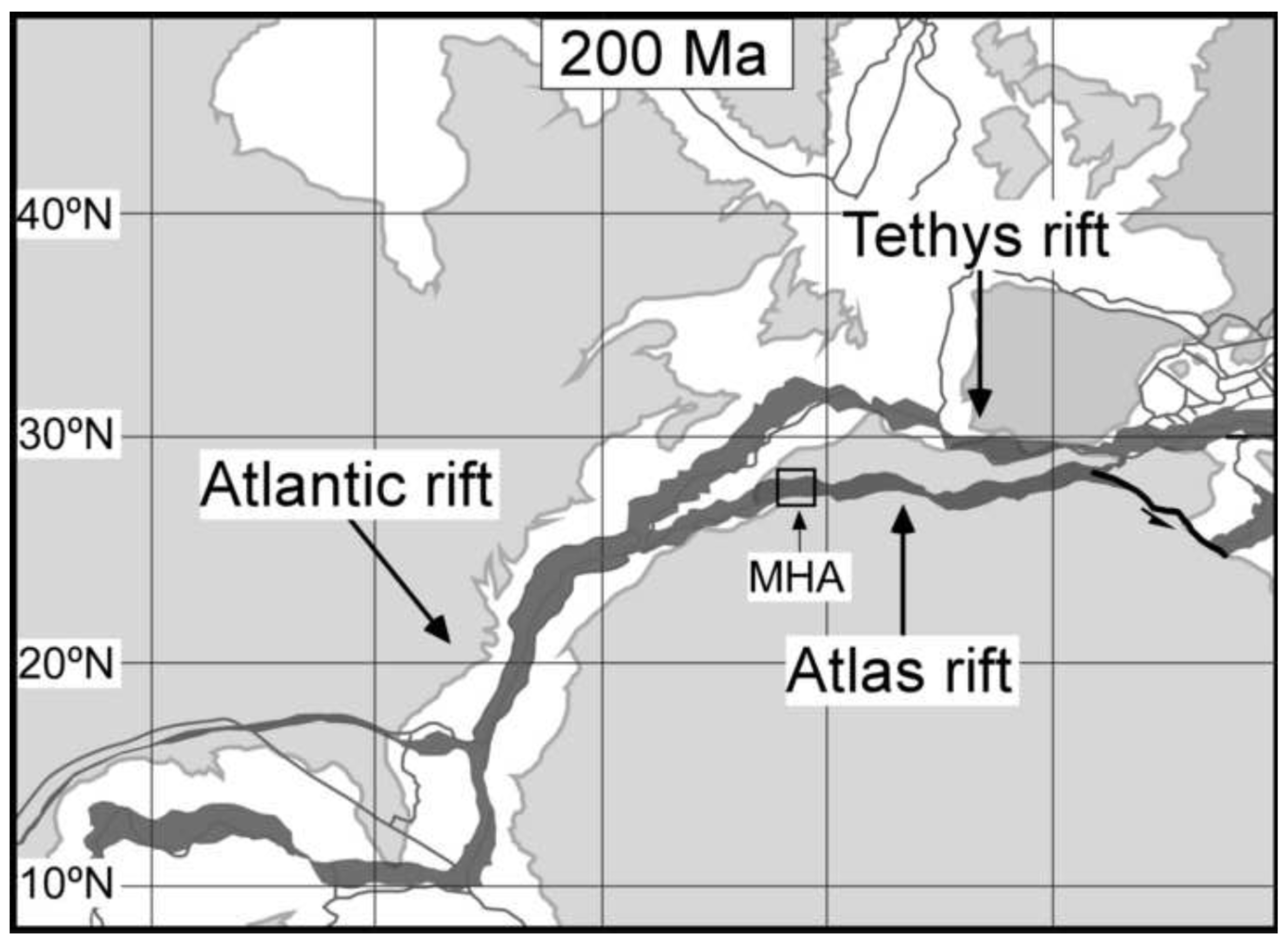
Plate reconstruction of the Central Atlantic to the Triassic-Jurassic boundary (200 Ma) (modified from Schettino and Turco, 2009). Rift zones are shown in dark grey. The square indicates the reconstructed position of the Marrakech High Atlas pf Morocco (MHA).
(Domènech et al., 2015)
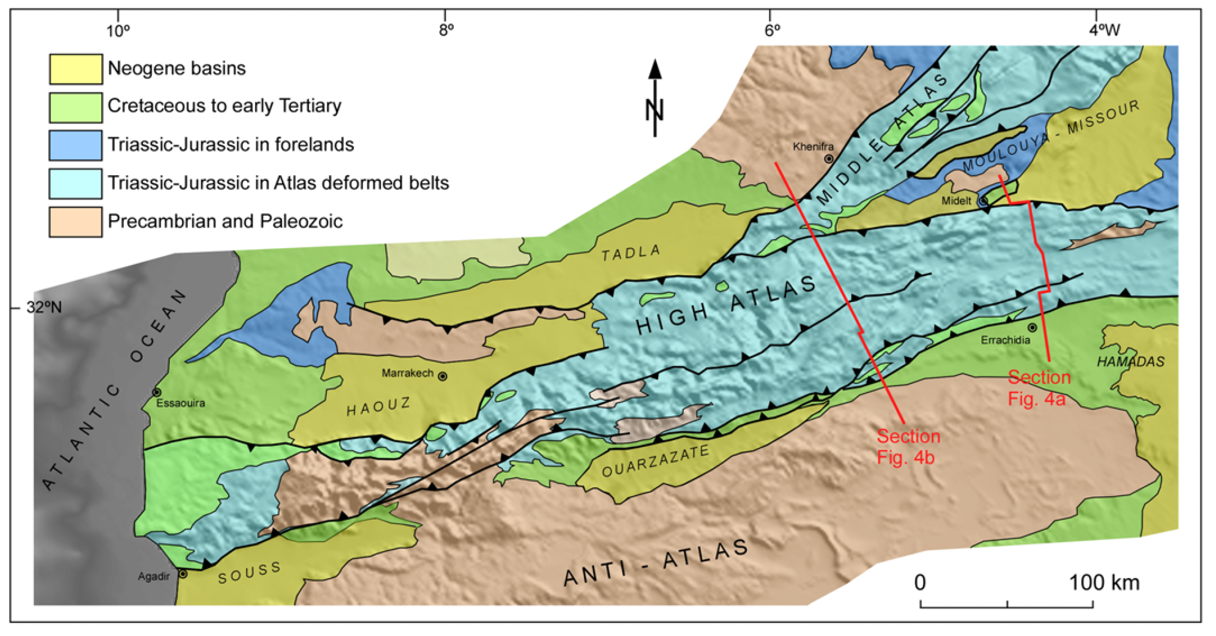
Tectonic sketch map of the Moroccan High Atlas Mountains, indicating the lines of section of Figure 4a, b.
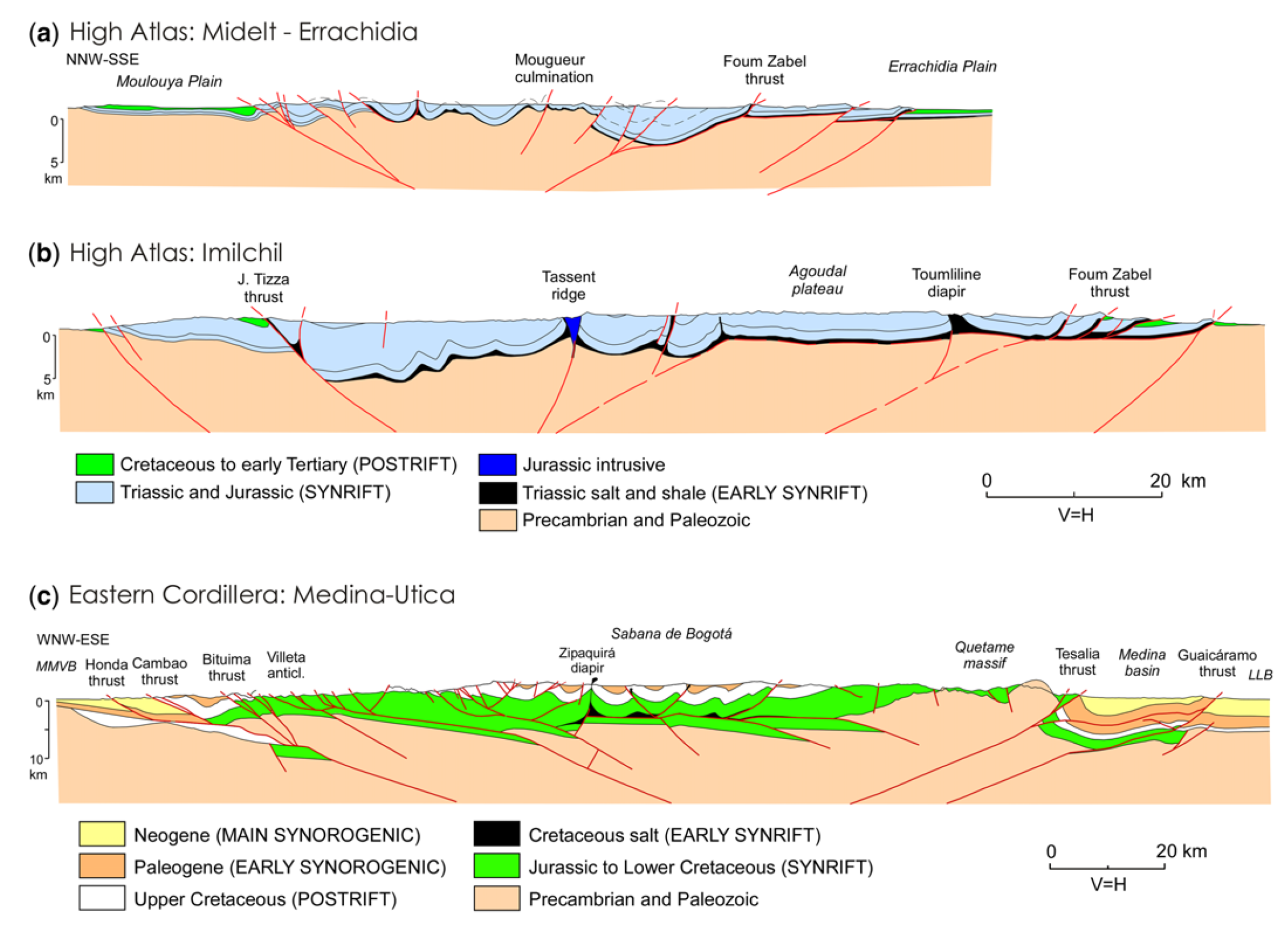
Structural cross-sections across the High Atlas and the Eastern Cordillera of Colombia. (a, b) Sections across the eastern and central High Atlas (from Teixell et al. 2003). These sections are based on field data and were modified from the original according to gravity modelling by Ayarza et al. 2005 (see location in Fig. 1). Although largely eroded, the Cretaceous sediments probably formed a tabular body that covered the entire Atlas domain, representing post-rift conditions. (c) Simplified structural cross-section of the Eastern Cordillera of Colombia, approximately through the latitude of Bogota´ (see location in Fig. 2). This section was constructed on the basis of maps, seismic profiles and structural data provided by ICP-Ecopetrol. The deep structure of the Sabana de Bogota´ region is conjectural as it is poorly imaged in the seismic profiles. The lower–upper Cretaceous boundary is taken for the sake of convenience at the top of the Une and Hilo´ formations. MMVB, Middle Magdalena Valley basin; LLB, Llanos basin.
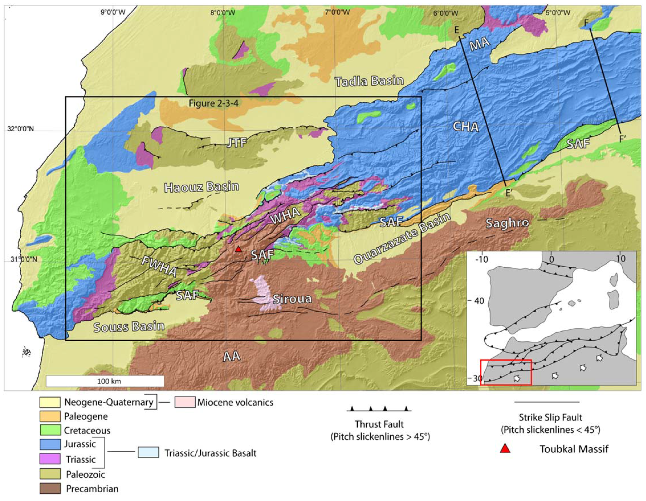
Location of the study area and simplified geological map of the High Atlas and Anti‐Atlas Mountains. Africa Plate motion considering Eurasia fixed by Serpelloni et al. (2007). FWHA = far western High Atlas; WHA = western High Atlas; CHA = central High Atlas, AA = Anti‐Atlas; MA = Middle Atlas; SAF = South Atlas fault; JTF = Jebilet thrust front.
Simplified geological map of the study area with schematic logs. See Figure 1 for location. The black lines are the cross‐section traces. Data from Baudon et al. (2009), Domènech et al. (2016, 2015), and El Arabi et al. (2003).
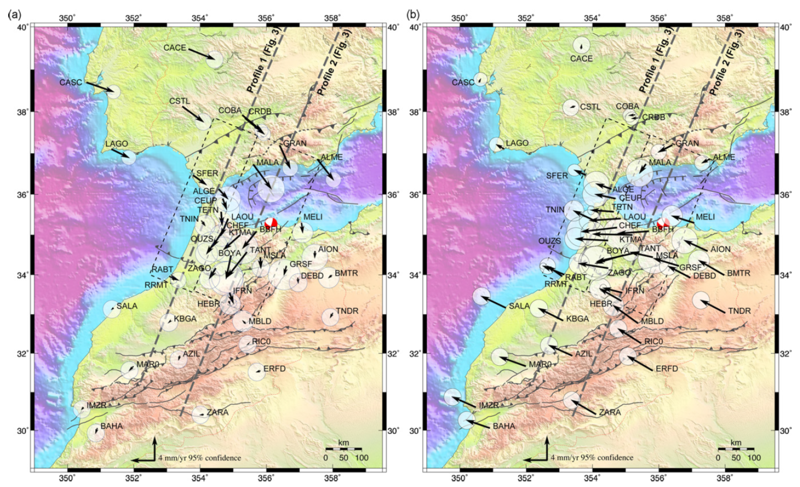
(a) GPS site velocities with respect to Nubia and 95% confidence ellipses. Heavy dashed lines show locations of profiles shown in Fig. 3 with the widths of the profiles indicated by lighter dashed lines. Focal mechanism indicates the location of the February 2004 Al Hoceima earthquake. Base map as in Fig. 1. (b) GPS site velocities with respect to Eurasia and 95% confidence ellipses. Format as in (a).
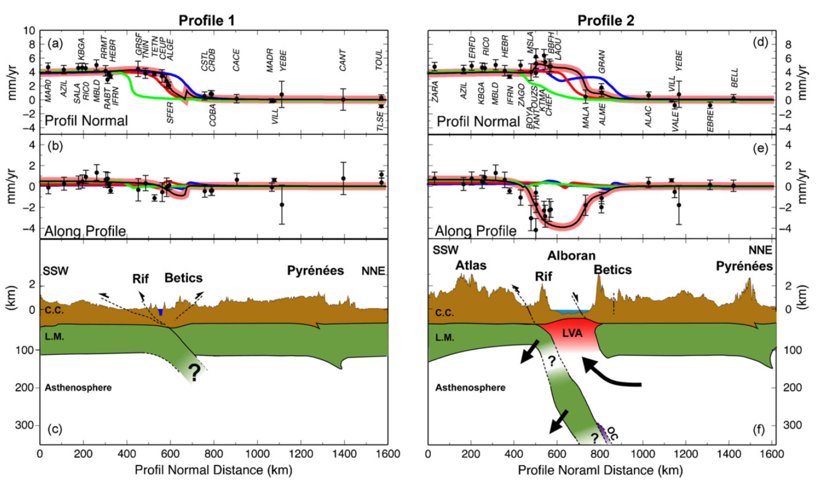
Profiles 1 and 2 (see Fig. 2a). (a and d) Component of velocities and 1-sigma uncertainties along the direction of plate motion (normal to profile). (b and e) Component of velocities and 1-sigma uncertainties normal to the direction of plate motion (i.e., parallel to profiles). The interseismic deformation predicted by elastic block models is shown for the three main hypothesized plate boundaries (Red = Klitgord and Schouten, 1986; Green = Bird, 2003; Blue = Gutscher, 2004, see Fig. 1 for geometry). The pink line is for a model with a central Rif block (see the figure for geometry). (c and f) Topography and interpretative cross-section along Profiles 1 and 2. CC = Continental crust, LM= lithospheric mantle, OC= ocean crust, LVA = low velocity, high attenuation seismic anomaly (Calvert et al., 2000a,b).
UPDATE: 11 Sept 2023
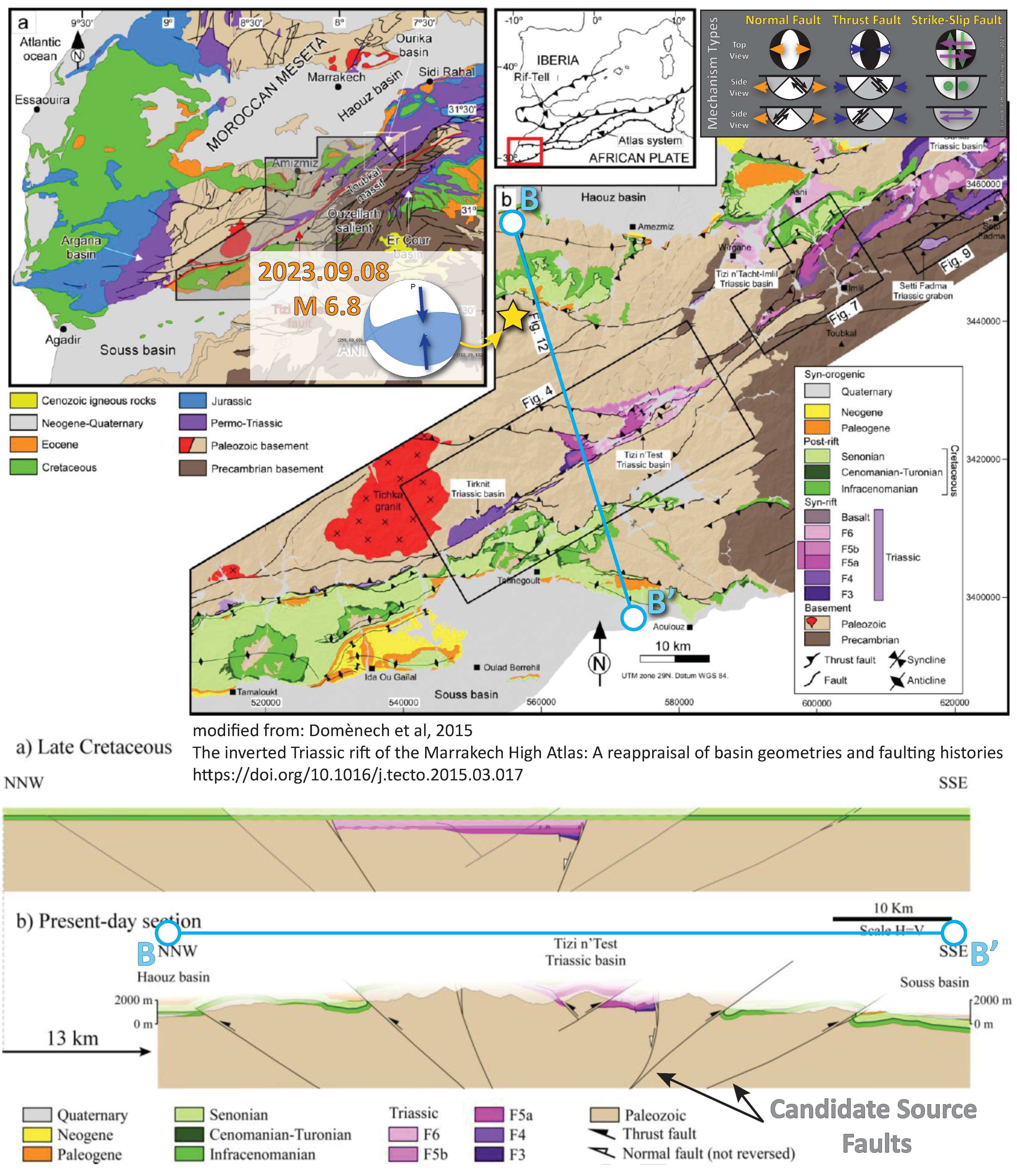
(a) Geologic map of the western and Marrakech High Atlas (modified from Hollard, 1985), showing location of the study area detailed in (b). (b) Geologic map of the Marrakech High Atlas showing the main structural elements. Squares correspond to areas described in detail in this paper.
Present-day cross section of the Marrakech High Atlas (see location in Fig. 2) and restoration to a state previous to the orogenic inversion in the Late Cretaceous.
Seismic Hazard and Seismic Risk
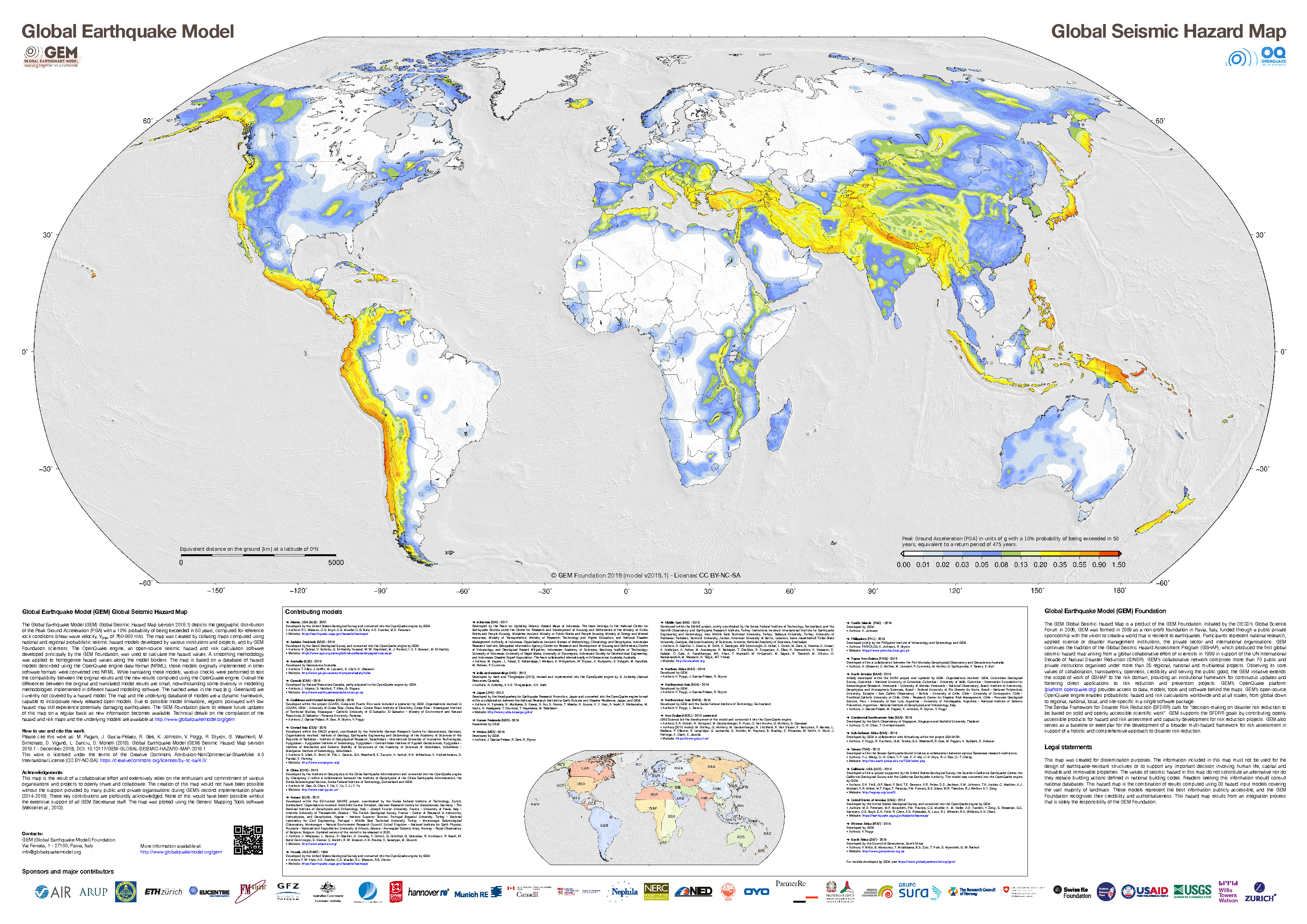
- These are the two maps that show seismic and seismic risk for the western Mediterranean, the GEM Seismic Hazard and the GEM Seismic Risk maps from Pagani et al. (2018) and Silva et al. (2018).
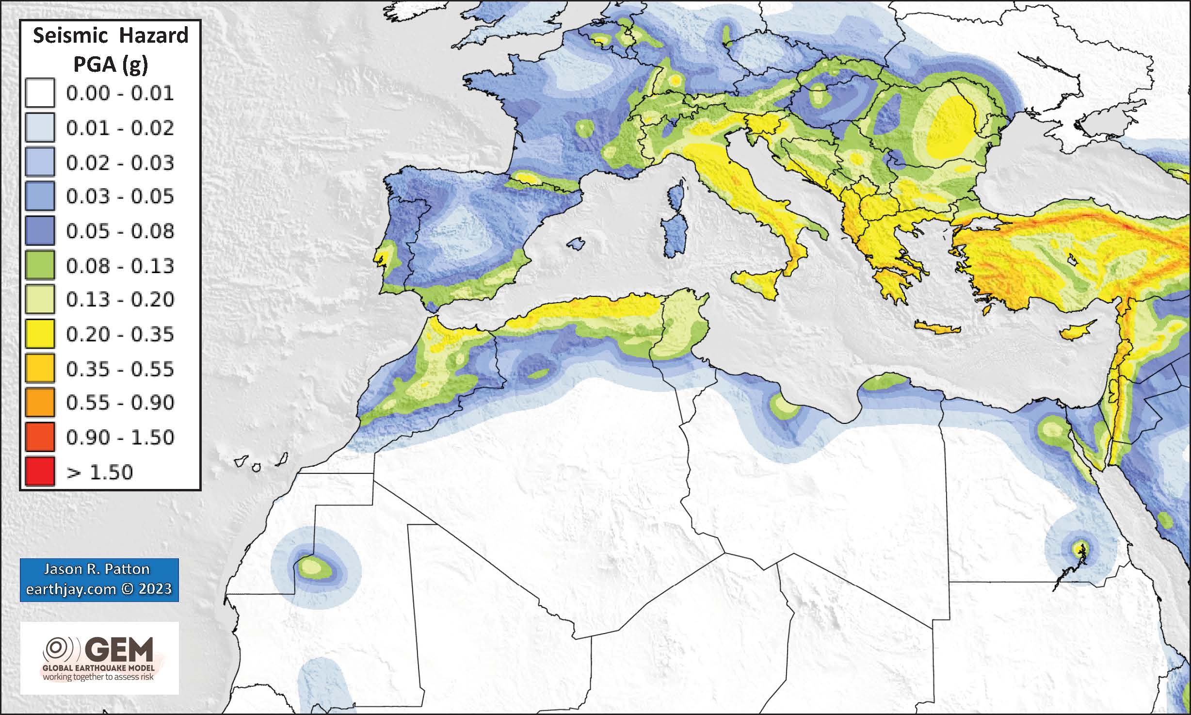
- The GEM Seismic Hazard Map:
- The Global Earthquake Model (GEM) Global Seismic Hazard Map (version 2018.1) depicts the geographic distribution of the Peak Ground Acceleration (PGA) with a 10% probability of being exceeded in 50 years, computed for reference rock conditions (shear wave velocity, VS30, of 760-800 m/s). The map was created by collating maps computed using national and regional probabilistic seismic hazard models developed by various institutions and projects, and by GEM Foundation scientists. The OpenQuake engine, an open-source seismic hazard and risk calculation software developed principally by the GEM Foundation, was used to calculate the hazard values. A smoothing methodology was applied to homogenise hazard values along the model borders. The map is based on a database of hazard models described using the OpenQuake engine data format (NRML). Due to possible model limitations, regions portrayed with low hazard may still experience potentially damaging earthquakes.
- Here is a view of the GEM seismic hazard map for the western Mediterranean.
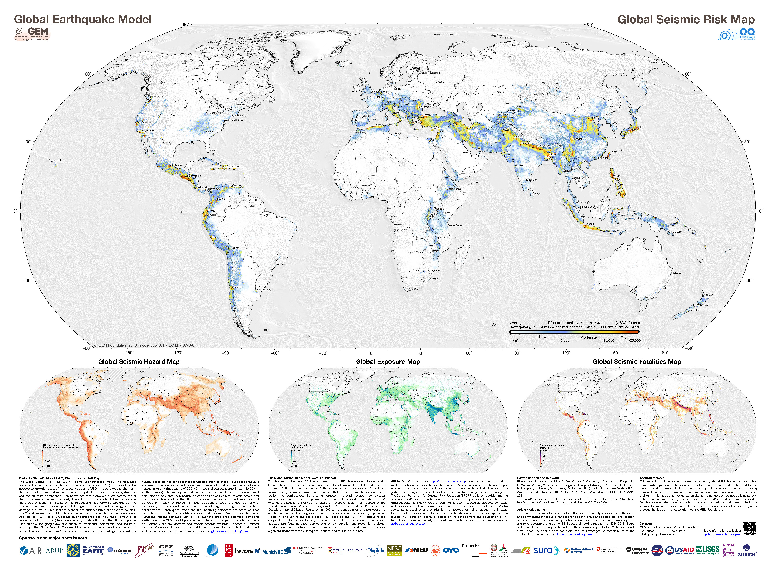
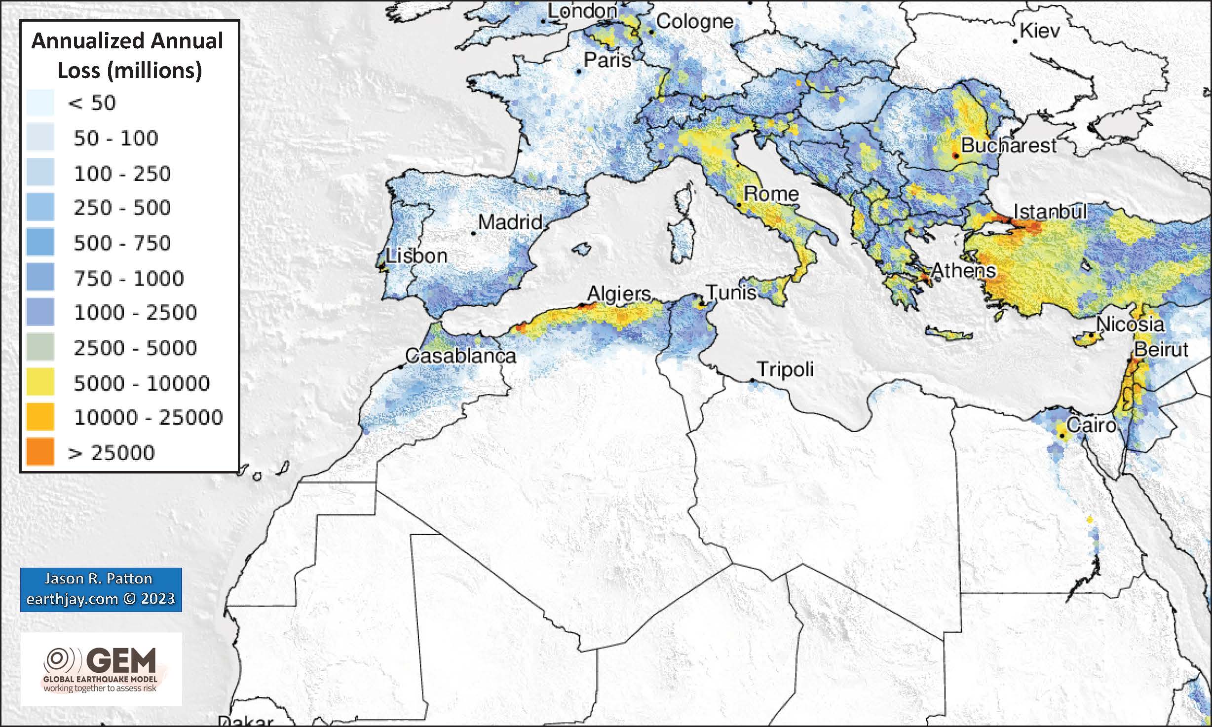
- The GEM Seismic Risk Map:
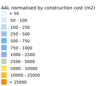
- The Global Seismic Risk Map (v2018.1) presents the geographic distribution of average annual loss (USD) normalised by the average construction costs of the respective country (USD/m2) due to ground shaking in the residential, commercial and industrial building stock, considering contents, structural and non-structural components. The normalised metric allows a direct comparison of the risk between countries with widely different construction costs. It does not consider the effects of tsunamis, liquefaction, landslides, and fires following earthquakes. The loss estimates are from direct physical damage to buildings due to shaking, and thus damage to infrastructure or indirect losses due to business interruption are not included. The average annual losses are presented on a hexagonal grid, with a spacing of 0.30 x 0.34 decimal degrees (approximately 1,000 km2 at the equator). The average annual losses were computed using the event-based calculator of the OpenQuake engine, an open-source software for seismic hazard and risk analysis developed by the GEM Foundation. The seismic hazard, exposure and vulnerability models employed in these calculations were provided by national institutions, or developed within the scope of regional programs or bilateral collaborations.
- Here is a view of the GEM seismic risk map for the western Mediterranean.
- 2023.09.08 M 6.8 Morocco
- 2018.05.15 M 5.8 Madagascar
- 2018.03.08 M 5.6 Mozambique and Malawi
- 2017.04.03 M 6.5 Botswana
- 2016.9.10 M 5.7 Tanzania
- Frisch, W., Meschede, M., Blakey, R., 2011. Plate Tectonics, Springer-Verlag, London, 213 pp.
- Hayes, G., 2018, Slab2 – A Comprehensive Subduction Zone Geometry Model: U.S. Geological Survey data release, https://doi.org/10.5066/F7PV6JNV.
- Holt, W. E., C. Kreemer, A. J. Haines, L. Estey, C. Meertens, G. Blewitt, and D. Lavallee (2005), Project helps constrain continental dynamics and seismic hazards, Eos Trans. AGU, 86(41), 383–387, , https://doi.org/10.1029/2005EO410002. /li>
- Jessee, M.A.N., Hamburger, M. W., Allstadt, K., Wald, D. J., Robeson, S. M., Tanyas, H., et al. (2018). A global empirical model for near-real-time assessment of seismically induced landslides. Journal of Geophysical Research: Earth Surface, 123, 1835–1859. https://doi.org/10.1029/2017JF004494
- Kreemer, C., J. Haines, W. Holt, G. Blewitt, and D. Lavallee (2000), On the determination of a global strain rate model, Geophys. J. Int., 52(10), 765–770.
- Kreemer, C., W. E. Holt, and A. J. Haines (2003), An integrated global model of present-day plate motions and plate boundary deformation, Geophys. J. Int., 154(1), 8–34, , https://doi.org/10.1046/j.1365-246X.2003.01917.x.
- Kreemer, C., G. Blewitt, E.C. Klein, 2014. A geodetic plate motion and Global Strain Rate Model in Geochemistry, Geophysics, Geosystems, v. 15, p. 3849-3889, https://doi.org/10.1002/2014GC005407.
- Meyer, B., Saltus, R., Chulliat, a., 2017. EMAG2: Earth Magnetic Anomaly Grid (2-arc-minute resolution) Version 3. National Centers for Environmental Information, NOAA. Model. https://doi.org/10.7289/V5H70CVX
- Müller, R.D., Sdrolias, M., Gaina, C. and Roest, W.R., 2008, Age spreading rates and spreading asymmetry of the world’s ocean crust in Geochemistry, Geophysics, Geosystems, 9, Q04006, https://doi.org/10.1029/2007GC001743
- Pagani,M. , J. Garcia-Pelaez, R. Gee, K. Johnson, V. Poggi, R. Styron, G. Weatherill, M. Simionato, D. Viganò, L. Danciu, D. Monelli (2018). Global Earthquake Model (GEM) Seismic Hazard Map (version 2018.1 – December 2018), DOI: 10.13117/GEM-GLOBAL-SEISMIC-HAZARD-MAP-2018.1
- Silva, V ., D Amo-Oduro, A Calderon, J Dabbeek, V Despotaki, L Martins, A Rao, M Simionato, D Viganò, C Yepes, A Acevedo, N Horspool, H Crowley, K Jaiswal, M Journeay, M Pittore, 2018. Global Earthquake Model (GEM) Seismic Risk Map (version 2018.1). https://doi.org/10.13117/GEM-GLOBAL-SEISMIC-RISK-MAP-2018.1
- Storchak, D. A., D. Di Giacomo, I. Bondár, E. R. Engdahl, J. Harris, W. H. K. Lee, A. Villaseñor, and P. Bormann (2013), Public release of the ISC-GEM global instrumental earthquake catalogue (1900–2009), Seismol. Res. Lett., 84(5), 810–815, doi:10.1785/0220130034.
- Zhu, J., Baise, L. G., Thompson, E. M., 2017, An Updated Geospatial Liquefaction Model for Global Application, Bulletin of the Seismological Society of America, 107, p 1365-1385, https://doi.org/0.1785/0120160198
- Here is an update to the reference list: https://doi.org/10.1016/j.jsg.2020.104021
- Arboleya, M.L., Teoxe;. A., Charroud, M., Julivert, M., 2004. A structural transect through the High and Middle Atlas of Morocco in Journal of African Earth Sciences, v. 39, p. 319-327, https://doi.org/10.1016/j.jafrearsci.2004.07.036
- Beauchamp, W., Allmendinger, R.W., Barazangi, M., Demnati, A., El Alji, M., and Dahmani, M., 1999. Inversion tectonics and the evolution of the High Atlas Mountains, Morocco, based on a geological-geophysical transect in Tectonics, v. 18, no. 2, p. 163-184, https://doi.org/10.1029/1998TC900015
- Domènech, M., Teixell, A., Babault, J., and Arbolya, M-L., 2015. The inverted Triassic rift of the Marrakech High Atlas: A reappraisal of basin geometries and faulting histories in Tectonophysics, v. 663, p. 177-191, https://doi.org/10.1016/j.tecto.2015.03.017
- Domènech, M., Teixell, A., and Stockli, D.F., 2016. Magnitude of rift-related burial and orogenic contraction in the Marrakech High Atlas revealed by zircon(U-Th)/He thermochronology and thermal modeling in Tectonics, v. 35, p. 2609–2635, https://doi.org/10.1002/2016TC004283
- Jiménez‐Munt, I., M. Fernàndez, J. Vergés, D. Garcia‐Castellanos, J. Fullea, M. Pérez‐Gussinyé, and J. C. Afonso(2011), Decoupled crust‐mantle accommodation of Africa‐Eurasia convergence in the NW Moroccan margin,J. Geophys. Res.,116, B08403, https://doi.org/10.1029/2010JB008105
- Babault, J., Teixell, A., Struth, L., Van Den Driessche, J., Arboleya, ML., Tesón, and E., 2013. “Shortening, structural relief and drainage evolution in inverted rifts: insights from the Atlas Mountains, the Eastern Cordillera of Colombia and the Pyrenees”, Thick-Skin-Dominated Orogens: From Initial Inversion to Full Accretion, in Nemcˇok, M., Mora, A. & Cosgrove, J. W. (eds) Thick-Skin-Dominated Orogens: From Initial Inversion to Full Accretion. Geological Society, London, Special Publications, 377, http://dx.doi.org/10.1144/SP377.14
- Lanari, R., Faccenna, C., Fellin, M. G., Essaifi, A., Nahid, A., Medina, F., & Youbi, N. (2020). Tectonic evolution of the western High Atlas of Morocco: Oblique convergence, reactivation, and transpression. Tectonics, 39, e2019TC005563. https://doi.org/10.1029/2019TC005563
- Teixell, A., Arboleya, M., Julivert, M., and Charroud, M., 2003. Tectonic shortening and topography in the central High Atlas (Morocco) in Tectonics, v. 22, no. 5, 1051, https://doi.org/10.1029/2002TC001460
- Vernant et al., 2010. Geodetic constraints on active tectonics of the Western Mediterranean: Implications for the kinematics and dynamics of the Nubia-Eurasia plate boundary zone in Journal of Geodynamics, v. 49, no 3-4, p. 123-129, https://doi.org/10.1016/j.jog.2009.10.007
- Sorted by Magnitude
- Sorted by Year
- Sorted by Day of the Year
- Sorted By Region

Africa
Earthquake Reports
Social Media
#EarthquakeReport for M6.8 #Earthquake in #Morroco
Looks like it will be quite damaging and may lead to a large number of casualties
Reported intensity MMI 7
Hopefully suffering is minimalhttps://t.co/mO3uGkOkeK pic.twitter.com/JEOnKz4kpc— Jason "Jay" R. Patton (@patton_cascadia) September 8, 2023
#EarthquakeReport for M6.8 #Earthquake in #Morocco
high intensity (reported at least MMI 9)
associated with tectonics of the Atlas Mountainsread report here:https://t.co/D6VNcSBjWS pic.twitter.com/uzvloTTa9B
— Jason "Jay" R. Patton (@patton_cascadia) September 9, 2023
#EarthquakeReport for M6.8 #Earthquake in #Morocco
updated @USGS_Quakes intensity and ground failure data and earthquake slip estimate
read report here:https://t.co/D6VNcSBjWS pic.twitter.com/p6vukhjgVn
— Jason "Jay" R. Patton (@patton_cascadia) September 10, 2023
The recent M6.8 earthquake in Morocco is the largest ever recorded in the country – and news reports indicate that it was deadly.
What happened? Why? What can we expect next? Read more in our blog, Earthquake Insights. Find the link in my bio. pic.twitter.com/FQQBdhzgCs
— Dr. Judith Hubbard (@JudithGeology) September 9, 2023
Mw=6.9, MOROCCO (Depth: 24 km), 2023/09/08 22:11:01 UTC – Full details here: https://t.co/WoG8zWb5j2 pic.twitter.com/cdypxjgAjO
— Earthquakes (@geoscope_ipgp) September 8, 2023
Prelim. M6.8 in Morocco, about 50 miles southwest of Marrakesh. That's a sizeable population center. USGS estimates over 2 million people were exposed to "strong to very strong" shaking. Fatalities and building damages are sadly expected. #earthquake #morocco pic.twitter.com/V0DVrSho04
— Brian Olson (@mrbrianolson) September 8, 2023
Recent shallow 6.8 Mw (#Morocco 🇲🇦) Western High Atlas, oblique reverse faulting. pic.twitter.com/1T6IxJRyBW
— Abel Seism🌏Sánchez (@EQuake_Analysis) September 8, 2023
For sure the causative structure is related to Atlas, however, the preliminary focal mechanism suggests also a N122 trending structure, which may correspond to an oblique structure that is subtle but visible in the satellite imagery. Cannot find literature on this. pic.twitter.com/la7a8t1Ym5
— Dr. Paula M Figueiredo (@paleoquake.bsky.social) (@pm_figueiredo) September 9, 2023
Just half an hour ago, Mw6.8 #earthquake in Morocco, not far from Agadir.
Very shallow and very large for that area (the tragic Agadir 1960 EQ was just M5.9)
Felt over a very large area, including Portugal, Spain and Algeria.
Dangerous!https://t.co/cFfpsUSS9c pic.twitter.com/WLU5c686sT— José R. Ribeiro (@JoseRodRibeiro) September 8, 2023
#Earthquake 76 km SW of #Marrakech (#Morocco) 29 min ago (local time 23:11:00). Updated map – Colored dots represent local shaking & damage level reported by eyewitnesses. Share your experience:
📱https://t.co/bKBgMenA4F
🌐https://t.co/lZLiJgtzeF pic.twitter.com/GYCSBv0zT6— EMSC (@LastQuake) September 8, 2023
This is a raw seismogram of the Mw 6.8 High Atlas, Morocco Earthquake which hit about 4.5 hours ago. It is recorded on a seismograph located ~115km east, at Tiouine (where a dam was built in 2013 to provide water for Ouarzazate). The seismograph is recorded many tiny aftershocks pic.twitter.com/ybi1fayxO6
— Jamie Gurney 🇬🇧🇳🇿 (@UKEQ_Bulletin) September 9, 2023
M 6.8 – 56 km W of Oukaïmedene, Morocco https://t.co/Vy54y0q0vc pic.twitter.com/VHLPmgMWS3
— Wendy Bohon, PhD 🌏 (@DrWendyRocks) September 8, 2023
A complex plate boundary separates the African Plate from the Eurasian Plate, skirting the northern edges of Algeria & Morocco. Today's M6.8 was not in the middle of a tectonic plate, but neither was it immediately along an active plate boundary. pic.twitter.com/wZ82Z5sUn6
— Dr. Susan Hough 🦖 (@SeismoSue) September 8, 2023
3 looks at the M6.8 Morocco earthquake: data from a seismometer in Rabat, past earthquakes in the region, and local plate motion relative to Eurasia (pink scale arrow is 25 mm/yr).
Explore for yourself ⬇️https://t.co/yZeORNrlN6https://t.co/XKHNEprsTchttps://t.co/0P2wufC5ez pic.twitter.com/Igsjwp6OJ4— EarthScope Consortium (@EarthScope_sci) September 9, 2023
WATCH: 6.8-magnitude earthquake hits Morocco, killing more than 300 people pic.twitter.com/sOHj2HRSMs
— BNO News (@BNONews) September 9, 2023
— Jason "Jay" R. Patton (@patton_cascadia) September 9, 2023
Reports of damage after 6.8-magnitude earthquake hits Morocco pic.twitter.com/tQqYsosW8x
— BNO News (@BNONews) September 8, 2023
Preliminary M7.0 #Earthquake
ID: #rs2023rspqys
31km/19miles from #OuladBerhil, in #Morocco
2023-09-08 22:10 UTC@raspishake networkJoin the largest #CitizenScience #seismograph community ➡ https://t.co/Y5O0dgJqJF
EVENT ➡ https://t.co/TPA2YZeitu pic.twitter.com/9lj9vO1oPw
— Raspberry Shake Earthquake Channel (@raspishakEQ) September 8, 2023
Schweres Erdbeben mit Magnitude 6.9 im Zentrum von Marokko, etwa mittig zwischen Marrakech und Agadir. Spürbar bis weit nach Spanien und Portugal. Mit Abstand das stärkste Erdbeben in der Geschichte von Marokko (auf dem Festland). Viele Opfer zu befürchten. pic.twitter.com/A57vM45hcF
— Erdbebennews (@Erdbebennews) September 8, 2023
By reminding that SCENARIOS ARE NOT REAL DATA, that could also significantly differ, this is what (and when) we expect from #InSAR for the M 6.8 #moroccoearthquake, both planes
First Sentinel-1 data in 2 days
more here: https://t.co/70vbRGVzxm@antandre71 @maferp_13 @FraxInSAR pic.twitter.com/ei873ucSmd— Simone Atzori (@SimoneAtzori73) September 9, 2023
Creo que aún no somos conscientes de que acabamos de sobrevivir al terremoto más grande de la historia de marruecos. Nosotros estamos aún en shock, pero bien. No se como describir lo que estamos viviendo #terremotomarruecos #terremoto #earthquake #Marrakech #terremotomarrakech pic.twitter.com/4Ac64w86NS
— Juan Bilbao (@joanbilbao93) September 9, 2023
Recent Earthquake Teachable Moment for the M6.8 earthquake in Morocco.
Teachable Moments presentations capture the opportunity to bring knowledge, insight, and critical thinking to the classroom following a newsworthy earthquake.
➡️ https://t.co/oZ08dRr8A8 pic.twitter.com/oU66f6sv7f
— EarthScope Consortium (@EarthScope_sci) September 9, 2023
רעידת אדמה עוצמתית במרוקו 🇲🇦, החזקה ביותר שתועדה שם! שרשור גיאולוגי מתגלגל. נתחיל במיקום- כמו שאפשר לראות במפה הטופוגרפית הזאת, הרעידה קרתה בשולי אזור הררי. אזור זה נקרא הרי האטלס הגבוהים (High atlas) והוא אחד ממספר תתי רכסים שמרכיבים את הרי האטלסhttps://t.co/P80eBHCY36
— Tom (@Karnafush) September 9, 2023
How did the ground shake in Morocco? The most immediate data can come from contributed felt reports, from which we estimate "intensities" that indicate the severity of shaking.
A 🧵https://t.co/VjwM1LiKwM
#earthquake #Morocco— Dr. Susan Hough 🦖 (@SeismoSue) September 9, 2023
Hi everyone – we're looking to make our posts more accessible to impacted people.
Here is a link to our post via Google Translate; choose your preferred language: https://t.co/02gDh9ZBni
If you want to help generate more accurate versions in Arabic/Berber/French, DM me! https://t.co/Tr60gdbf8J
— Dr. Judith Hubbard (@JudithGeology) September 9, 2023
At least 1,000 people were killed and 1,200 injured after a 6.8-magnitude earthquake shook Morocco late Friday, the Interior Ministry said. The earthquake struck in the province of Al Haouz, about 43 miles south of Marrakesh, devastating buildings and sending panicked residents… pic.twitter.com/xrQxizRMBA
— The Washington Post (@washingtonpost) September 9, 2023
You can find images of destruction submitted to the EMSC here: https://t.co/T6ZCHSBhdh
If you live in the region and felt shaking, consider submitting your own description. This helps guide scientific analysis of the event and its impacts: https://t.co/PtinNqMLGu
— Dr. Judith Hubbard (@JudithGeology) September 9, 2023
This is the story. The link of reactivation of the Atlas to the dragging I figured out this morning, so is not in this paper :)
— Douwe van Hinsbergen (@vanHinsbergen) September 9, 2023
Information on the M6.8 earthquake in Morocco, including video showing the seismic waves from that event as detected in North America.
My heart goes out to everyone impacted by this tragedy. pic.twitter.com/TkoQyKAqUS
— Wendy Bohon, PhD 🌏 (@DrWendyRocks) September 9, 2023
Powerful earthquake hits Morocco 😢 😢😢
Recorded across New England.@westportskyguys @jpulli @BCSchillerInst pic.twitter.com/1mdEqtPApD— Alan Kafka (@Weston_Quakes) September 9, 2023
#Séisme au Maroc : « Sa survenue dans cette région n’est pas une surprise » mes explications dans @lemondefr https://t.co/hlCkOCMukY
— Robin Lacassin – @RobinLacassin@qoto.org (@RLacassin) September 9, 2023
6.8-magnitude-earthquake-triggered landslide has swept away the town of Adassil in the Moroccan Atlas. >7000 people live there. pic.twitter.com/iXQ773kEpz
— Δρ(García-Castellanos) (@danigeos) September 10, 2023
Sections showing responses on @raspishake citizen seismometers across the globe, to yesterday's deadly M6.8 earthquake in Morocco. On the 0-180° section, a response can be seen in Wellington, NZ. On the 0-95° section, filtered at 0.1-10Hz, there are PcP reflections from the core. pic.twitter.com/26hLx0yNVt
— Mark Vanstone (@wmvanstone) September 10, 2023
While earthquakes in western Morocco are rare and there have been no other M6+ quakes since 1900, many residences in the area are vulnerable to shaking and earthquake impacts can be severe. In 1960, the M5.8 Agadir earthquake killed 12,000-15,000 people in coastal Morocco.
— USGS Earthquakes (@USGS_Quakes) September 9, 2023
It's been a day and a half since the earthquake in Morocco, and we're starting to learn more.
Landslides caused damage and are complicating rescue efforts. Aftershocks hint at a possible fault geometry. Satellite images are pending.
Read more on our blog; link in my bio. https://t.co/Tr60gdbf8J pic.twitter.com/fjZr1nQM1m
— Dr. Judith Hubbard (@JudithGeology) September 10, 2023
The Tinmal Mosque, a historical structure dating back to the 12th century located in the High Atlas mountains of Morocco and renowned for its Almohad architecture, has been reduced to ruins in the aftermath of the devastating earthquake. pic.twitter.com/ijALCucM97
— Morocco World News (@MoroccoWNews) September 9, 2023
I tried to look at the correlation between the location of aftershocks (according to EMSC) and coulomb stress change using the @USGS_Quakes model. Not a good overlap, but informative. @JudithGeology Maybe some insights for your previous blog today. pic.twitter.com/iECjFlPZeR
— Achraf (@KoulaliAchraf) September 14, 2023
The comparison between observed and modeled data for track 154 (descending, left) and track 45 (ascending, right).
Previous model tweet: https://t.co/d52hngYRzV pic.twitter.com/uLYzKgEl81
— Simone Atzori (@SimoneAtzori73) September 16, 2023
How did the earthquake in Morocco change the shape of the High Atlas mountains – and how do we know? In our latest post, we explain InSAR, and what it can – and can't – tell us.
Read more on our blog; the link is in my bio (and in the image below). pic.twitter.com/AkXQ5KxMB2
— Dr. Judith Hubbard (@JudithGeology) September 21, 2023
References:
Basic & General References
Specific References
Return to the Earthquake Reports page.