Earthquake Report: Gulf of Alaska UPDATE #1

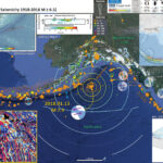
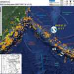
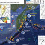
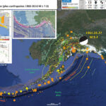
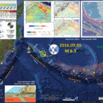
Well. What a firestorm of social media discusions about this earthquake. It seems that, like how we learn so much when earthquakes like this happen, the amount of interacting in public on social media has been growing earthquake by earthquake.
I spent some time this afternoon looking at the magnetic anomalies, after taking a load of a part of an old building to the county dump (transfer station) before the rain started. Stephen Hicks found a great paper (and tweeted about it, see my original report here where I include his tweet).
UPDATES Below is a list of all the reports associated with this earthquake sequence.

In my original report, I proposed that if the earthquake happened on the USGS fault model, then there is a problem when considering the magnetic anomaly map. The USGS fault solution is left-lateral, but the magnetic anomaly offsets appear to be right-laterally offset. Upon further review, I noticed that there are some details in this area that could be interpreted as left lateral. In my poster below, I place a white arrow along the hypothetical fault (drawn as a green dashed line). I located the line based upon offsets in the magnetic anomaly data as aligned with the USGS model.
Then I took a look at the mag anomaly map from Naugler and Wageman (1973). These authors show the isochrons for the Gulf of Alaska (GA). The fracture zone nearest today’s M 7.9 earthquake is right-lateral (supporting my original interpretation). However, the USGS fault model appears to be oblique to this fracture zone. Perhaps today’s M 7.9 is on a conjugate fault, with a different sense of motion.
Interesting that the USGS fault model terminates on the eastern side with the epicenter from a 1999 earthquake. This earthquake has a fault plane solution that shows oblique slip, not pure strike-slip. This could be because (1) the earthquake happened on a different fault or (2) the earthquake happened on the same fault, but the fault is changing its orientation (I favor the first hypothesis).
Some people have been stating that the aftershocks appear to be aligned in a north-south orientation. I cannot figure out how they made this observation, but maybe I am missing something. This did make me think about instances where off fault earthquakes can be triggered, or when there are major fault systems that are not reflected in the geomorphology nor other measures of long term tectonics (like magnetic anomalies or fracture zones). A great example is the 2012 M 8.6 Wharton Basin earthquakes that ruptured in response to the 2004 Sumatra-Andaman subduction zone earthquake eight years earlier. Today’s M 7.9 earthquake is rather deep (like the 2012 earthquakes), so perhaps there are some deep faults that are not reflected by the shape of the seafloor nor reflected by the gravity data for some reason (the former seems more likely to me).

Below is my interpretive poster for this earthquake

I plot the seismicity from the past month, with color representing depth and diameter representing magnitude (see legend). I include earthquake epicenters from 1918-2018 with magnitudes M ≥ 6.5. More about the plate boundary can be found in that report.
I plot the USGS fault plane solutions (moment tensors in blue and focal mechanisms in orange) for the M 7.9 earthquake, in addition to some relevant historic earthquakes.

  • I placed a moment tensor / focal mechanism legend on the poster. There is more material from the USGS web sites about moment tensors and focal mechanisms (the beach ball symbols). Both moment tensors and focal mechanisms are solutions to seismologic data that reveal two possible interpretations for fault orientation and sense of motion. One must use other information, like the regional tectonics, to interpret which of the two possibilities is more likely.
  • I also include the shaking intensity contours on the map. These use the Modified Mercalli Intensity Scale (MMI; see the legend on the map). This is based upon a computer model estimate of ground motions, different from the “Did You Feel It?” estimate of ground motions that is actually based on real observations. The MMI is a qualitative measure of shaking intensity. More on the MMI scale can be found here and here. This is based upon a computer model estimate of ground motions, different from the “Did You Feel It?” estimate of ground motions that is actually based on real observations.
  • I include the slab contours plotted (Hayes et al., 2012), which are contours that represent the depth to the subduction zone fault. These are mostly based upon seismicity. The depths of the earthquakes have considerable error and do not all occur along the subduction zone faults, so these slab contours are simply the best estimate for the location of the fault. Slab 2.0 is due out later this year!
  • I include some inset figures.

  • In the lower right corner, I place a map from Naugler and Sageman (1973). I added relative slip vectors for the fracture zones here. I place the epicenter from today’s earthquake as a cyan star.


  • As I was rereading my report (don’t always get a chance, but good to check for typos), looking at the aftershocks, and considering the problems associated with this earthquake and its tectonic setting (i.e. right-lateral fracture zones and a left-lateral USGS fault solution), I decided to make some updates to this large scale poster. There were several aftershocks while I was making this map that made a north-south trend more apparent. So, now I am favoring the following interpretation: the M 7.9 mainshock and many aftershocks are the result of a right-lateral north-striking strike-slip fault.
  • This is the exact same thing that happened following the 2012 Wharton Basin M 8.6/8.2 earthquake sequence along the outer rise of the Sumatra-Andaman subduction zone. The M 8.6 is the largest strike-slip intraplate earthquake ever recorded on modern seismometers. I present some maps from Sumatra earthquakes below. Basically, the fracture zones in the the India-Australia plate trend north-south. So that was my initial interpretation, that these earthquakes were left-lateral earthquakes on faults associated with these fracture zones. However, this was not the case. The Wharton Basin earthquake sequence involved both fracture zone related faults, in addition to conjugate faults trending east-west. There were initially fault slip models for both interpretations.


Some Relevant Discussion and Figures

  • This is a great map from UNAVCO. This shows the static offsets to GPS sites as a result of this M 7.9 earthquake.

  • Seismically derived static displacements (first figure, pink is p1 and blue is p2) and their difference (figure 2)(Figure/Dave Mencin, UNAVCO)

  • Here are some interpretive posters from the 2012 Sumatra Outer Rise earthquake sequence.
  • I have presented materials related to the 2004 Sumatra-Andaman subduction zone earthquake here and more here.
  • I include a map in the upper right corner that shows the historic earthquake rupture areas. There is a figure from Meng et al. (2012) that shows the details about the faults and the seismicity.

  • Here is that Meng et al. (2012) figure showing the different faults that ruptured in 2012.

  • Here is a poster that shows some earthquakes in the Andaman Sea. This is from my earthquake report from 2015.11.08.

  • This map shows the fracture zones in the India-Australia plate.

Review Stuff from my first report.

  • Here is a map for the earthquakes of magnitude greater than or equal to M 7.0 between 1900 and 2016. This is the USGS query that I used to make this map. One may locate the USGS web pages for all the earthquakes on this map by following that link.

Social Media

Earthquake Report: Gulf of Alaska!

I was asleep in bed, trying to catch up to prevent myself from getting ill, when there was a large earthquake in the Gulf of Alaska (GA), offshore of Kodiak, Alaska. When I wakened, I noticed a fb message from my friend Scott Willits notifying me of an M 8.2 earthquake in Alaska, posted at 2:20 AM local time. I immediately got up to check on this and was surprised that there was not a tsunami evacuation going on. I live in the small town of Manila (population ~700), on the North Spit (a sand spit west of Arcata and Eureka, CA). I live above 10 m in elevation and do not consider myself exposed to tsunami risks, local or distant (especially given that (1) the CSZ locked zone is mostly under land here and (2) that the part of the locked zone that is not under land is in shallow water; so our local tsunami will probably be much smaller than further north, like Crescent City or Brookings). I have been involved in tsunami education and outreach for over 15 years and prepared the first tsunami hazard map for northern CA (working with Dr. Lori Dengler and the Redwood Coast Tsunami Work Group). Needless to say, I am cogent and aware about the tsunami risk here in norcal.

https://earthquake.usgs.gov/earthquakes/eventpage/us2000cmy3/executive

SO. I soon discovered that the GA earthquake happened in the Pacific plate, far from the subduction zone and that the earthquake was a strike-slip earthquake. Both of these facts explained why the sheriff had not been at my door earlier this morning. In addition, the magnitude had been adjusted to M 7.9 (no longer a Great earthquake, just a Large earthquake; earthquake classes are defined here). However, there were some small tsunami waves observed (see below) as reported by the National Tsunami Warning Center (see social media below).
This earthquake appears to be located along a reactivated fracture zone in the GA. There have only been a couple earthquakes in this region in the past century, one an M 6.0 to the east (though this M 6.0 was a thrust earthquake). The Gulf of Alaska shear zone is even further to the east and has a more active historic fault history (a pair of earthquakes in 1987-1988). The magnetic anomalies (formed when the Earth’s magnetic polarity flips) reflect a ~north-south oriented spreading ridge (the anomalies are oriented north-south in the region of today’s earthquake). There is a right-lateral offset of these magnetic anomalies located near the M 7.9 epicenter. Interesting that this right-lateral strike-slip fault (?) is also located at the intersection of the Gulf of Alaska shear zone and the 1988 M 7.8 earthquake (probably just a coincidence?). However, the 1988 M 7.8 earthquake fault plane solution can be interpreted for both fault planes (it is probably on the GA shear zone, but I don’t think that we can really tell).
This is strange because the USGS fault plane is oriented east-west, leading us to interpret the fault plane solution (moment tensor or focal mechanism) as a left-lateral strike-slip earthquake. So, maybe this earthquake is a little more complicated than first presumed. The USGS fault model is constrained by seismic waves, so this is probably the correct fault (east-west).
I prepared an Earthquake Report for the 1964 Good Friday Earthquake here.
UPDATES Below is a list of all the reports associated with this earthquake sequence.

Below is my interpretive poster for this earthquake

I plot the seismicity from the past month, with color representing depth and diameter representing magnitude (see legend). I include earthquake epicenters from 1918-2018 with magnitudes M ≥ 6.5. More about the plate boundary can be found in that report.
I plot the USGS fault plane solutions (moment tensors in blue and focal mechanisms in orange) for the M 7.9 earthquake, in addition to some relevant historic earthquakes.

  • I placed a moment tensor / focal mechanism legend on the poster. There is more material from the USGS web sites about moment tensors and focal mechanisms (the beach ball symbols). Both moment tensors and focal mechanisms are solutions to seismologic data that reveal two possible interpretations for fault orientation and sense of motion. One must use other information, like the regional tectonics, to interpret which of the two possibilities is more likely.
  • I also include the shaking intensity contours on the map. These use the Modified Mercalli Intensity Scale (MMI; see the legend on the map). This is based upon a computer model estimate of ground motions, different from the “Did You Feel It?” estimate of ground motions that is actually based on real observations. The MMI is a qualitative measure of shaking intensity. More on the MMI scale can be found here and here. This is based upon a computer model estimate of ground motions, different from the “Did You Feel It?” estimate of ground motions that is actually based on real observations.
  • I include the slab contours plotted (Hayes et al., 2012), which are contours that represent the depth to the subduction zone fault. These are mostly based upon seismicity. The depths of the earthquakes have considerable error and do not all occur along the subduction zone faults, so these slab contours are simply the best estimate for the location of the fault. Slab 2.0 is due out later this year!
  • I include some inset figures.

  • In the upper left corner, I place a map created by Dr. Peter Haeussler, USGS, which shows the historic earthquakes along the Alaska and Aleutian subduction zones. I place the epicenter from today’s earthquake as a cyan star.
  • To the right of this map, I include first the USGS map that shows their interpretation of where the fault is (the red line) and then I include the USGS fault slip model (color = slip in meters).
  • In the upper right corner is a map from IRIS that shows seismicity with color representing depth.
  • In the lower right corner, I include a low angle oblique view of the subduction zone, showing how the Pacific plate is subducting beneath the North America plate.
  • In the lower left corner, I include a map that shows the magnetic anomalies in the GA region. I include USGS seismicity from 1918-2018 for earthquakes M ≥ 5.5.


  • UPDATE 12:45 my local time
  • The USGS updated their MMI contours to reflect their fault model. Below is my updated poster. I also added green dashed lines for the fracture zones related to today’s M 7.9 earthquake (on the magnetic anomaly inset map).


  • These are the observations as reported by the NTWC this morning (at 4:15 AM my local time).

  • Here is an educational video from IRIS about the tectonics in Alaska.

Some Relevant Discussion and Figures

  • Here is a map for the earthquakes of magnitude greater than or equal to M 7.0 between 1900 and 2016. This is the USGS query that I used to make this map. One may locate the USGS web pages for all the earthquakes on this map by following that link.

  • Here is a cross section showing the differences of vertical deformation between the coseismic (during the earthquake) and interseismic (between earthquakes).

  • Here is a figure recently published in the 5th International Conference of IGCP 588 by the Division of Geological and Geophysical Surveys, Dept. of Natural Resources, State of Alaska (State of Alaska, 2015). This is derived from a figure published originally by Plafker (1969). There is a cross section included that shows how the slip was distributed along upper plate faults (e.g. the Patton Bay and Middleton Island faults).

  • There are three types of earthquakes, strike-slip, compressional (reverse or thrust, depending upon the dip of the fault), and extensional (normal). Here is are some animations of these three types of earthquake faults. Many of the earthquakes people are familiar with in the Mendocino triple junction region are either compressional or strike slip. The following three animations are from IRIS.
  • Strike Slip:
  • Compressional:
  • Extensional:
  • This figure shows what a transform plate boundary fault is. Looking down from outer space, the crust on either side of the fault moves side-by-side. When one is standing on the ground, on one side of the fault, looking across the fault as it moves… If the crust on the other side of the fault moves to the right, the fault is a “right lateral” strike slip fault. The Mendocino and San Andreas faults are right-lateral (dextral) strike-slip faults. I believe this is from Pearson Higher Ed.

  • For more on the graphical representation of moment tensors and focal mechnisms, check this IRIS video out:
  • Here is a fantastic infographic from Frisch et al. (2011). This figure shows some examples of earthquakes in different plate tectonic settings, and what their fault plane solutions are. There is a cross section showing these focal mechanisms for a thrust or reverse earthquake. The upper right corner includes my favorite figure of all time. This shows the first motion (up or down) for each of the four quadrants. This figure also shows how the amplitude of the seismic waves are greatest (generally) in the middle of the quadrant and decrease to zero at the nodal planes (the boundary of each quadrant).

Social Media

Earthquake Report: Bering fracture zone: UPDATE #1

Well, based upon a comment on twitter, I thought it prudent to review the seismicity of this region at the westernmost part of the western Aleutian Islands. For many years I considered this region part of the subduction zone that forms the Aleutian Trench. In the past couple of years, there have been a number of earthquakes that reveal this to not be the case. Rather, the Pacific-North America plate boundary in this region is in the form of a shear zone, distributed across several reactivated fracture zones. I noticed a plot from Jascha Polet and found another article that evaluates this plate boundary (Davaille and Lees, 2004).
Here is my initial #EarthquakeReport on this M 7.7 strike-slip earthquake.
Here is a report from the University of Alaska Fairbanks, Alaska Earthquake Center.

Below is my interpretive poster for this earthquake.

  • I placed a moment tensor / focal mechanism legend on the poster. There is more material from the USGS web sites about moment tensors and focal mechanisms (the beach ball symbols). Both moment tensors and focal mechanisms are solutions to seismologic data that reveal two possible interpretations for fault orientation and sense of motion. One must use other information, like the regional tectonics, to interpret which of the two possibilities is more likely. I plot moment tensors for the M 7.7 earthquake. Based upon the series of earthquakes and the mapped faults, I interpret this M 7.7 earthquake as a right-lateral strike-slip earthquake related to slip associated with the Bering fracture zone.
  • I also include the shaking intensity contours on the map. These use the Modified Mercalli Intensity Scale (MMI; see the legend on the map). This is based upon a computer model estimate of ground motions, different from the “Did You Feel It?” estimate of ground motions that is actually based on real observations. The MMI is a qualitative measure of shaking intensity. More on the MMI scale can be found here and here. This is based upon a computer model estimate of ground motions, different from the “Did You Feel It?” estimate of ground motions that is actually based on real observations.
  • I include the slab contours plotted (Hayes et al., 2012), which are contours that represent the depth to the subduction zone fault. These are mostly based upon seismicity. The depths of the earthquakes have considerable error and do not all occur along the subduction zone faults, so these slab contours are simply the best estimate for the location of the fault.
  • I plot the seismicity from the past month, with color representing depth and diameter representing magnitude (see legend). I also include USGS earthquake epicenters from 1917-2017 for magnitudes M ≥ 5.0. The depths for these earthquakes is represented by color. This is quite revealing when considering whether subduction is occurring in this part of the plate boundary. Note how earthquakes east of Attu Island have hypocentral depths (3-dimensional location of the earthquake focus) that extend to over 150 km. These represent earthquakes in the downgoing Pacific plate. We also observe earthquakes even deeper along the Kamchatka Trench on the west. Also note that the slab contours (Hayes et al., 2012) have decreasing maximum depths from east to west between Bowers Ridge and Attu Island. The same is true for the subduction zone beneath Kamchatka, though the cut-off of these depth contours is more abrupt (due to the tear in the Pacific plate, which marks the edge of the subduction zone beneath Kamchatka). Finally, note how the earthquake depths in the region between Attu Island and Kamchatka are largely less than 33 km.

    I include some inset figures in the poster.

  • In the upper left corner I include a regional tectonic map showing Kamchatka and the westernmost tip of the westernmost Aleutian Islands (Davaille and Lees, 2004).
  • In the lower right corner I show a schematic illustration that depicts how the subduction transitions to strike-slip in the region of the Attu Island (Davaille and Lees, 2004).
  • To the right is a large scale map of this region showing the complicated intersection of strike slip and compressional tectonics as the tip of the Aleutians intersects with Kamchatka (Gaedicke et al., 2000).
  • In the upper right corner is a figure showing seismicity in this region (Davaille and Lees, 2004). There is a map (with earthquakes plotted vs. depth in color) and several cross sections (one parallel to the Kamchatka trench and two normal/perpendicular to the trench). Note how the depths for the earthquakes shallow to the north of the Meiji Seamount, and particularly shallower to the north of the Stellar fault (a.k.a. Bering Kresla Shear zone) and the Bering fault (a.k.a. Bering fracture zone).


  • Here is my original #EarthquakeReport Interpretive Poster and report.

  • Here is the seismicity plot from Davaille and Lees (2000). They suspect that the tear in the Pacific plate is related to the interaction of a mantle plume hotspot and the oceanic lithosphere as it is formed near this hotspot. I include their figure caption below in blockquote.

  • Seismicity in Kamchatka. (a) Mapview showing earthquakes plotted with colors corresponding to depth. Projections of the Bering and Steller faults onto Kamchatka are presented for clarity and reference. (b–d) Vertical cross-sections of seismicity in Kamchatka. Magenta circles are from the Gorbatov et al. [3] catalog and yellow events are from the Engdahl et al. [52] catalog. The projection of the subducting Meiji seamounts is shaded gray.

  • Here is a plot from Jascha Polet, seismologist at Cal Poly Pomona. These data are consistent with the Davaille and Lees (2000) plot, showing shallow seismicity in this region of the plate boundary.

  • Here is the low-angle oblique map from Portnyagin and Manea (2008). This was in my original report, but is a great visualization for this interpretation of the Pacific plate tear (the edge of subduction in Kamchatka). While this is not evidence for the lack of subduction in the region of the Bering Kresla Shear zone, it does suggest that there is no active subduction beneath Kamchatka to the north. If this is the case (and I have no reason to think that it is not the case), there is little evidence for subduction west of Attu Island and east of Kamchatka. I include the figure caption as a blockquote below.

  • Kamchatka subduction zone. A: Major geologic structures at the Kamchatka–Aleutian Arc junction. Thin dashed lines show isodepths to subducting Pacific plate (Gorbatov et al., 1997). Inset illustrates major volcanic zones in Kamchatka: EVB—Eastern Volcanic Belt; CKD—Central Kamchatka Depression (rift-like tectonic structure, which accommodates the northern end of EVB); SR—Sredinny Range. Distribution of Quaternary volcanic rocks in EVB and SR is shown in orange and green, respectively. Small dots are active vol canoes. Large circles denote CKD volcanoes: T—Tolbachik; K l — K l y u c h e v s k o y ; Z—Zarechny; Kh—Kharchinsky; Sh—Shiveluch; Shs—Shisheisky Complex; N—Nachikinsky. Location of profiles shown in Figures 2 and 3 is indicated. B: Three dimensional visualization of the Kamchatka subduction zone from the north. Surface relief is shown as semi-transparent layer. Labeled dashed lines and color (blue to red) gradation of subducting plate denote depths to the plate from the earth surface (in km). Bold arrow shows direction of Pacific Plate movement.

  • Here is another great visualization of the subducting slabs in this region, prepared by Lees et al. (2007). This figure shows isosurfaces (surfaces of equal value of some parameter, like seismic velocity, or Vp:Vs ratios; Vp = P-Wave velocity, Vs = S-Wave velocity). These isosurfaces were created using seismic tomography, which is basically just like a CT scan of the earth. CT stands for “computed tomography” of X-Rays. The mathematical solutions used in these methods are the same, even though the source of the data are different (X-Rays vs. seismic waves). Coastlines are in grey outline. Kamchatka is labelled M. The lower panel may be easier to look at first because north is up. Basically, blue is old and cold and red is young and hot. So, the downgoing Pacific plate is in blue and the surrounding mantle is in red. Note how the blue blobs end in the area of interest.

  • Tomographic image of the Kamchatka Subduction zone rendered in three-dimensions. The cut-off perturbation level is 3% with blue regions being high velocity and red lower velocity perturbations. The slab is a clear high velocity zone approximately 100 km thick plunging into the upper mantle at an angle of ~50. The green plane represents the top of the subduction zone seismicity, contoured and rendered along with the tomographic images. Gold cones are active volcanoes along the Kamchatka arc and white squares are stations included for reference to the map in Figure 1. The bars represent length scales of 100 km. Points of interest discussed in the text are marked with letters (I–M).

  • Finally of note (unrelated to the previous discussion) is that this M 7.7 had a really long duration (Dr. Polet pointed this out in a tweet). This plot is from IPGP here. The source time function represents how much energy is released over time. Time is on the horizontal axis.

    References:

  • Bassett and Watts, 2015. Gravity anomalies, crustal structure, and seismicity at subduction zones: 1. Seafloor roughness and subducting relief in Geochemistry, Geophysics, Geosystems, v. 16, doi:10.1002/2014GC005684.
  • Davaille, A. and Lees, J.M., 2004. Thermal modeling of subducted plates: tear and hotspot at the Kamchatka corner in EPSL, v. 226, p. 293-304.
  • Gaedicke, C., Baranov, B., Seliverstov, N., Alexeiev, D., Tsukanov, N., Freitag, R., 2000. Structure of an active arc-continent collision area: the Aleutian-Kamchatka junction. Tectonophysics 325, 63–85
  • Hayes, G. P., D. J. Wald, and R. L. Johnson (2012), Slab1.0: A three-dimensional model of global subduction zone geometries, J. Geophys. Res., 117, B01302, doi:10.1029/2011JB008524.
  • Ikuta, R., Mitsui, Y., Kurokawa, Y., and Ando, M., 2015. Evaluation of strain accumulation in global subduction zones from seismicity data in Earth, Planets and Space, v. 67, DOI 10.1186/s40623-015-0361-5
  • Konstantnovskaia, 2001. Arc-continent collision and subduction reversal in the Cenozoic evolution of the Northwest Pacific: an example from Kamchatka (NE Russia) in Tectonophysics, v. 333, p. 75-94.
  • Koulakov, I.Y., Dobretsov, N.L., Bushenkova, N.A., and Yakovlev, A.V., 2011. Slab shape in subduction zones beneath the Kurile–Kamchatka and Aleutian arcs based on regional tomography results in Russian Geology and Geophysics, v. 52, p. 650-667.
  • Krutikov, L., et al., 2008. Active Tectonics and Seismic Potential of Alaska, Geophysical Monograph Series 179, doi:10.1029/179GM07
  • Lees, J.M., VanDecar, J., Gordeev, E., Ozerov, A., Brandon, M., Park, J., and Levvin, V, 2007. Three Dimensional Images of the Kamchatka-Pacific Plate Cusp in Volcanism and Subduction: The Kamchatka Region Geophysical Monograph Series 172, DOI: 10.1029/172GM06
  • Portnyagin, M. and Manea, V.C., 2008. Mantle temperature control on composition of arc magmas along the Central Kamchatka Depression in Geology, v. 36, no. 7, p. 519-522.
  • Rhea, S., Tarr, A.C., Hayes, G., Villaseñor, A., Furlong, K.P., and Benz, H.M., 2010. Seismicity of the Earth 1900-2007, Kuril-Kamchatka arc and vicinity: U.S. Geological Survey Open-File Report 2010-1083-C, 1 map sheet, scale 1:5,000,000.

Earthquake Report: Western Aleutians

We just had an earthquake along the western Aleutian Islands, very close to the international date line. In this region places often have more than two names, depending upon who drew the map.
The majority of the Aleutian Islands are volcanic arc islands formed as a result of the subduction of the Pacific plate beneath the North America plate. To the west, there is another subduction zone along the Kuril and Kamchatka volcanic arcs. These subduction zones form deep sea trenches (the deepest parts of the ocean are in subduction zone trenches). Between these 2 subduction zones is another linear trough, but this does not denote the location of a subduction zone. The plate boundary between the Kamchatka and Aleutian trenches is the Bering Kresla shear zone (BKSZ).
The oceanic basin, Komandorsky Basin, to the north of the BKSZ has been mapped with northwest trending fracture zones, most of which are fossil or inactive. However, due to the oblique convergence west of Bowers Ridge, some of these fossil fracture zones are being reactivated. Based upon offsets in magnetic anomalies in the oceanic crust forming the basement of Komandorsky Basin, these fracture zones show left-lateral offsets. However, the active strike-slip faults (and BKSZ) are right lateral. This is a great example of strike-slip faults reactivating as strike-slip faults.
The mainshock was preceded earlier this day with several foreshocks and occurred very close to a M 6.3 earthquake from 9 months ago (2016.09.05). In addition, there was seismic activity to the east about 6 weeks ago (2017.06.02 M 6.8).
Some place a tear in the downgoing Pacific plate (beneath Kamchatka) in the position of the Bering Kresla Shear zone. This marks the end of the modern Kamchatka subduction zone. However, there was a subduction zone further to the west of the active arc, which extended further to the north and possibly involved subduction of the oceanic crust forming the Komandorsky Basin. The combination of offsets along the right-lateral strike-slip faults to the north of the BKSZ, along with the convergence along the Kamchatka Trench, there is a fold and thrust belt (a zone of compressional tectonics). There was an M 6.6 earthquake earlier this year (2017.03.29), which is somewhat related to this fold and thrust belt.
Finally, of note, is the M 8.3 deep extensional earthquake in the downgoing Pacific plate crust (2013.05.24).
There was a tsunami recorded at the tide gage on Shemya Island, with an observed maximum wave height of 0.3 ft! This is interesting given the strike slip earthquake.

  • Here are the USGS website for today’s earthquakes.
  • 2017-07-17 11:05 M 6.2
  • 2017-07-17 11:23 M 5.1
  • 2017-07-17 23:34 M 7.7
  • Here are my #EarthquakeReport pages for some of these related earthquakes.
  • 2016.09.05 M 6.3
  • 2017.03.29 M 6.6
  • 2017.06.02 M 6.8

Below is my interpretive poster for this earthquake.

I plot the seismicity from the past month, with color representing depth and diameter representing magnitude (see legend). I also include USGS earthquake epicenters from 2007-2017 for magnitudes M ≥ 6.0.

  • I placed a moment tensor / focal mechanism legend on the poster. There is more material from the USGS web sites about moment tensors and focal mechanisms (the beach ball symbols). Both moment tensors and focal mechanisms are solutions to seismologic data that reveal two possible interpretations for fault orientation and sense of motion. One must use other information, like the regional tectonics, to interpret which of the two possibilities is more likely. I plot moment tensors for the M 7.7 earthquake, as well as for the 2013, 2016, and 2017 earthquakes mentioned above. I also include moment tensors for earthquakes in 1999 and 2001 because these are also interesting earthquakes that I had not noticed before. It appears that perhaps the 1999 strike-slip earthquake led to an increased stress on the subduction zone, which slipped in 2001. Based upon the series of earthquakes and the mapped faults, I interpret this M 7.7 earthquake as a right-lateral strike-slip earthquake related to slip associated with the Bering fracture zone.
  • I also include the shaking intensity contours on the map. These use the Modified Mercalli Intensity Scale (MMI; see the legend on the map). This is based upon a computer model estimate of ground motions, different from the “Did You Feel It?” estimate of ground motions that is actually based on real observations. The MMI is a qualitative measure of shaking intensity. More on the MMI scale can be found here and here. This is based upon a computer model estimate of ground motions, different from the “Did You Feel It?” estimate of ground motions that is actually based on real observations.
  • I include the slab contours plotted (Hayes et al., 2012), which are contours that represent the depth to the subduction zone fault. These are mostly based upon seismicity. The depths of the earthquakes have considerable error and do not all occur along the subduction zone faults, so these slab contours are simply the best estimate for the location of the fault.

    I include some inset figures in the poster.

  • In the upper left corner I include a regional tectonic map showing Kamchatka and the westernmost tip of the westernmost Aleutian Islands (Bindeman et a., 2002). Today’s M 7.7 earthquake is just off the map to the east.
  • To the right of the Bindeman map is a map that shows a larger scale view of the faults in this region (Gaedicke et al., 2000). I include an orange star designating the rough location of today’s M 7.7 earthquake.
  • In the lower left corner are the earthquake intensity regression plots for the M 6.2 and M 7.7 earthquakes. These are plots based upon Attenuation Relation equations (formerly called Ground Motion Prediction Equations, GMPEs). Using seismic data from thousands of earthquakes with a range of magnitudes, distances, fault types, etc., people have developed empirical relations between each of these parameters. These plots are based upon these empirical relations and show how earthquake intensity (how strong it shakes) diminishes with distance.
  • In the upper right corner is a series of tectonic maps showing one interpretation of how the plates have moved relative to each other through time (Konstantinovskaia, 2001). The time spans 65, 55, and 37 millions of years into the present. Begin by looking at the present configuration and move backwards in time. These maps show an interesting story (that appears consistent with other published data).


  • Here are several figures from Gaedicke et al. (2000) showing their tectonic reconstructions. I include their figure captions below in blockquote. The first map shows the general tectonic setting as in the poster above.

  • Map of the Aleutian–Bering region and location of the study area (rectangle). Lines with barbs indicate subduction zones: (1) Kamchatka Trench and (2) Aleutian Trench; lines with sense of displacement mark fracture zones (FZs): (3) Steller, (4) Pikezh and (5) Bering FZs. Single arrows show relative direction of convergence of the Pacific (P) and North American (NA) plates. Bathymetric contours are in meters.

  • This figure shows the complicated intersection of the BKSZ and the Kuril-Kamchatka Trench (a subduction zone).

  • The main tectonic features of the Kamchatka–Aleutian junction area modified from Seliverstov (1983), Seliverstov et al. (1988) and Baranov et al. (1991). The eastern side of the Central Kamchatka depression is bounded by normal faults. Contour interval is 1000 m. Lines A and B indicate the locations of profiles shown in Fig. 3; the rectangle marks the location of the area shown in Fig. 4.

  • This figure shows a medium scale view of the faults here, along with the major historic earthquakes. In this figure the BKSZ is labeled the Aleutian fracture zone (AFZ).

  • Rupture zones of the major earthquakes in the Kamchatka–Aleutian junction area [according to Vikulin (1997)]. Earthquakes with a magnitude of Mw>7 are shown.

  • Here are several figures from Konstantnovskaia et al. (2001) showing their tectonic reconstructions. I include their figure captions below in blockquote. The first figure is the one included in the poster above.

  • Geodynamic setting of Kamchatka in framework of the Northwest Pacific. Modified after Nokleberg et al. (1994) and Kharakhinov (1996)). Simplified cross-section line I-I’ is shown in Fig. 2. The inset shows location of Sredinny and Eastern Ranges. [More figure caption text in the publication].

  • Here are 4 panels that show the details of their reconstructions. Panels shown are for 65 Ma, 55 Ma, 37 Ma, and Present.


  • The Cenozoic evolution in the Northwest Pacific. Plate kinematics is shown in hotspot reference frame after (Engebretson et al., 1985). Keys distinguish zones of active volcanism (thick black lines), inactive volcanic belts (thick gray lines), deformed arc terranes (hatched pattern), subduction zones: active (black triangles), inactive *(empty triangles). In letters: sa = Sikhote-aline, bs = Bering shelf belts; SH = Shirshov Ridge; V = Vitus arch; KA = Kuril; RA = Ryukyu’ LA = Luzon; IBMA = Izu-Bonin-Mariana arcs; WPB = Western Philippine, BB = Bowers basins.

  • Here is the low-angle oblique map from Portnyagin and Manea (2008). I include the figure caption as a blockquote below.

  • Kamchatka subduction zone. A: Major geologic structures at the Kamchatka–Aleutian Arc junction. Thin dashed lines show isodepths to subducting Pacific plate (Gorbatov et al., 1997). Inset illustrates major volcanic zones in Kamchatka: EVB—Eastern Volcanic Belt; CKD—Central Kamchatka Depression (rift-like tectonic structure, which accommodates the northern end of EVB); SR—Sredinny Range. Distribution of Quaternary volcanic rocks in EVB and SR is shown in orange and green, respectively. Small dots are active vol canoes. Large circles denote CKD volcanoes: T—Tolbachik; K l — K l y u c h e v s k o y ; Z—Zarechny; Kh—Kharchinsky; Sh—Shiveluch; Shs—Shisheisky Complex; N—Nachikinsky. Location of profiles shown in Figures 2 and 3 is indicated. B: Three dimensional visualization of the Kamchatka subduction zone from the north. Surface relief is shown as semi-transparent layer. Labeled dashed lines and color (blue to red) gradation of subducting plate denote depths to the plate from the earth surface (in km). Bold arrow shows direction of Pacific Plate movement.

Earthquake Report: Westernmost Aleutian Arc

This earthquake happened a couple weeks ago, but was interesting and I have been looking forward to following up on this with a report. Here is the USGS website for this M 6.8 earthquake.
The M 6.8 earthquake happened in a region where the Pacific-North America plate boundary transitions from a subduction zone to a shear zone. To the east of this region, the Pacific plate subducts beneath the North America plate to form the Alaska-Aleutian subduction zone. As a result of this subduction, a deep oceanic trench is formed. To the west of this earthquake, the plate boundary is in the form of a shear zone composed of several strike-slip faults. The main fault that is positioned in the trench is the Bering-Kresla shear zone (BKSZ), a right-lateral strike-slip fault. In the oceanic basin to the north of the BKSZ there are a series of parallel fracture zones, also right-lateral strike-slip faults.
My initial thought is that the entire Aleutian trench was a subduction zone prior to about 47 million years ago (Wilson, 1963; Torsvik et al., 2017). Prior to 47 Ma, the relative plate motion in the region of the BKSZ would have been more orthogonal (possibly leading to subduction there). After 47 Ma, the relative plate motion in the region of the BKSZ has been parallel to the plate boundary, owing to the strike-slip motion here. However, Konstantinovskaia (2001) used paleomagnetic data for a plate motion reconstruction through the Cenozoic and they have concluded that there is a much more complicated tectonic history here (with strike-slip faults in the region prior to 47 Ma and other faults extending much farther east into the plate boundary). When considering this, I was reminded that the relative plate motion in the central Aleutian subduction zone is oblique. This results in strain partitioning where the oblique motion is partitioned into fault-normal fault movement (subduction) and fault-parallel fault movement (strike-slip, along forearc sliver faults). The magmatic arc in the central Aleutian subduction zone has a forearc sliver fault, but also appears to have blocks that rotate in response to this shear (Krutikov, 2008).
There have been several other M ~6 earthquakes to the west that are good examples of this strike-slip faulting in this area. On 2003.12.05 there was a M 6.7 earthquake along the Bering fracture zone (the first major strike-slip fault northeast of the BKSZ). On 2016.09.05 there was a M 6.3 earthquake also on the Bering fracture zone. Here is my earthquake report for the 2016 M 6.3 earthquake. The next major strike-slip fault, moving away from the BKSZ, is the right-lateral Alpha fracture zone. The M 6.8 earthquake may be related to this northwest striking fracture zone. However, aftershocks instead suggest that this M 6.8 earthquake is on a fault oriented in the northeast direction. There is no northeast striking strike-slip fault mapped in this area and the Shirshov Ridge is mapped as a thrust fault (albeit inactive). There is a left-lateral strike-slip fault that splays off the northern boundary of Bowers Ridge. If this fault strikes a little more counter-slockwise than is currently mapped at, the orientation would match the fault plane solution for this M 6.8 earthquake (and also satisfies the left-lateral motion for this orientation). The bathymetry used in Google Earth does not reveal the orientation of this fault, but the aftershocks sure align nicely with this hypothesis.

Below is my interpretive poster for this earthquake.

I plot the seismicity from the past month, with color representing depth and diameter representing magnitude (see legend). I also include USGS earthquake epicenters from 1997-2017 for magnitudes M ≥ 6.5.

  • I placed a moment tensor / focal mechanism legend on the poster. There is more material from the USGS web sites about moment tensors and focal mechanisms (the beach ball symbols). Both moment tensors and focal mechanisms are solutions to seismologic data that reveal two possible interpretations for fault orientation and sense of motion. One must use other information, like the regional tectonics, to interpret which of the two possibilities is more likely. I plot moment tensors for the M 6.8 earthquake, as well as for the 2003 and 2016 earthquakes mentioned above. I also include moment tensors for earthquakes in 1999 and 2001 because these are also interesting earthquakes that I had not noticed before. It appears that perhaps the 1999 strike-slip earthquake led to an increased stress on the subduction zone, which slipped in 2001. I will need to consider this earthquake pair more later. Here are the USGS websites for the 1999 and 2001 earthquakes.
  • I also include the shaking intensity contours on the map. These use the Modified Mercalli Intensity Scale (MMI; see the legend on the map). This is based upon a computer model estimate of ground motions, different from the “Did You Feel It?” estimate of ground motions that is actually based on real observations. The MMI is a qualitative measure of shaking intensity. More on the MMI scale can be found here and here. This is based upon a computer model estimate of ground motions, different from the “Did You Feel It?” estimate of ground motions that is actually based on real observations.
  • I include the slab contours plotted (Hayes et al., 2012), which are contours that represent the depth to the subduction zone fault. These are mostly based upon seismicity. The depths of the earthquakes have considerable error and do not all occur along the subduction zone faults, so these slab contours are simply the best estimate for the location of the fault. The hypocentral depth of the M 5.5 plots this close to the location of the fault as mapped by Hayes et al. (2012).

    I include some inset figures in the poster.

  • In the upper right corner is a figure that shows the historic earthquake ruptures along the Aleutian Megathrust (Peter Haeussler, USGS). I place a yellow star in the general location of this earthquake sequence (same for other figures here).
  • In the upper left corner is a figure from Gaedicke et al. (2000) which shows some of the major tectonic faults in this region.
  • In the lower right corner is a figure from Konstantnovskaia et al. (2001) that shows a very detailed view of all the faults in this complicated region.


  • On 2017.05.08 there was an earthquake further to the east, with a magnitude M 6.2. Here is my interpretive poster for this earthquake, which includes fault plane solutions for several historic earthquakes in the region. These fault plane solutions reveal the complicated intersection of these two different types of faulting along this plate boundary. Here is my earthquake report for this earthquake sequence.

  • Here is a map that shows some of the large earthquakes in this region from 1996 through 2015. Refer to the moment tensor legend to help interpret the moment tensors for each earthquake. All, but one, are compressional solutions. Note how all the compressional earthquakes have roughly the same strike, oriented relative to the plate convergence vectors (blue arrows). Note the fault plane solution and location for the 2014.06.23 M 7.2 earthquake. Do we see a trend here? This earthquake suggests the strike-slip faulting extends at least to the Bowers Ridge.

  • Here is a map that shows historic earthquake slip regions as pink polygons (Peter Haeussler, USGS). Dr. Haeussler also plotted the magnetic anomalies (grey regions), the arc volcanoes (black diamonds), and the plate motion vectors (mm/yr, NAP vs PP).

  • Here are several figures from Gaedicke et al. (2000) showing their tectonic reconstructions. I include their figure captions below in blockquote. The first map shows the general tectonic setting as in the poster above.

  • Map of the Aleutian–Bering region and location of the study area (rectangle). Lines with barbs indicate subduction zones: (1) Kamchatka Trench and (2) Aleutian Trench; lines with sense of displacement mark fracture zones (FZs): (3) Steller, (4) Pikezh and (5) Bering FZs. Single arrows show relative direction of convergence of the Pacific (P) and North American (NA) plates. Bathymetric contours are in meters.

  • This figure shows the complicated intersection of the BKSZ and the Kuril-Kamchatka Trench (a subduction zone).

  • The main tectonic features of the Kamchatka–Aleutian junction area modified from Seliverstov (1983), Seliverstov et al. (1988) and Baranov et al. (1991). The eastern side of the Central Kamchatka depression is bounded by normal faults. Contour interval is 1000 m. Lines A and B indicate the locations of profiles shown in Fig. 3; the rectangle marks the location of the area shown in Fig. 4.

  • This figure shows a medium scale view of the faults here, along with the major historic earthquakes. In this figure the BKSZ is labeled the Aleutian fracture zone (AFZ).

  • Rupture zones of the major earthquakes in the Kamchatka–Aleutian junction area [according to Vikulin (1997)]. Earthquakes with a magnitude of Mw>7 are shown.

  • Here is a great illustration that shows how forearc sliver faults form due to oblique convergence at a subduction zone (Lange et al., 2008). Strain is partitioned into fault normal faults (the subduction zone) and fault parallel faults (the forearc sliver faults, which are strike-slip). This figure is for southern Chile, but is applicable globally.

  • Proposed tectonic model for southern Chile. Partitioning of the oblique convergence vector between the Nazca plate and South American plate results in a dextral strike-slip fault zone in the magmatic arc and a northward moving forearc sliver. Modified after Lavenu and Cembrano (1999).

  • Here is a figure from Krutikov (2008) showing the block rotation and forearc sliver faults associated with the oblique subduction in the central Aleutian subduction zone. Note that there are blocks that are rotating to accommodate the oblique convergence. There are also margin parallel strike slip faults that bound these blocks. These faults are in the upper plate, but may impart localized strain to the lower plate, resulting in strike slip motion on the lower plate (my arm waving part of this). Note how the upper plate strike-slip faults have the same sense of motion as these deeper earthquakes.

  • Here is a figure that shows the plate age for seamounts in the Hawaii-Emperor Seamount Chain (Torsvik et al., 2017).

  • Hawaiian-Emperor Chain. White dots are the locations of radiometrically dated seamounts, atolls and islands, based on compilations of Doubrovine et al. and O’Connor et al. Features encircled with larger white circles are discussed in the text and Fig. 2. Marine gravity anomaly map is from Sandwell and Smith.

  • Here are several figures from Konstantnovskaia et al. (2001) showing their tectonic reconstructions. I include their figure captions below in blockquote. The first figure is the one included in the poster above.

  • Geodynamic setting of Kamchatka in framework of the Northwest Pacific. Modified after Nokleberg et al. (1994) and Kharakhinov (1996)). Simplified cross-section line I-I’ is shown in Fig. 2. The inset shows location of Sredinny and Eastern Ranges. [More figure caption text in the publication].

  • Here are 4 panels that show the details of their reconstructions. Panels shown are for 65 Ma, 55 Ma, 37 Ma, and Present.


  • The Cenozoic evolution in the Northwest Pacific. Plate kinematics is shown in hotspot reference frame after (Engebretson et al., 1985). Keys distinguish zones of active volcanism (thick black lines), inactive volcanic belts (thick gray lines), deformed arc terranes (hatched pattern), subduction zones: active (black triangles), inactive *(empty triangles). In letters: sa = Sikhote-aline, bs = Bering shelf belts; SH = Shirshov Ridge; V = Vitus arch; KA = Kuril; RA = Ryukyu’ LA = Luzon; IBMA = Izu-Bonin-Mariana arcs; WPB = Western Philippine, BB = Bowers basins.

Alaska | Kamchatka | Kurile

Earthquake Reports

  • 2017.06.02 M 6.8 Aleutians
  • 2017.05.08 M 6.2 Aleutians
  • 2017.05.01 M 6.3 British Columbia
  • 2017.03.29 M 6.6 Kamchatka
  • 2017.03.02 M 5.5 Alaska
  • 2016.09.05 M 6.3 Bering Kresla (west of Aleutians)
  • 2016.04.02 M 6.2 Alaska Peninsula
  • 2016.03.27 M 5.7 Aleutians
  • 2016.03.12 M 6.3 Aleutians
  • 2016.01.24 M 7.1 Alaska
  • 2015.11.09 M 6.2 Aleutians
  • 2015.11.02 M 5.9 Aleutians
  • 2015.11.02 M 5.9 Aleutians (update)
  • 2015.07.27 M 6.9 Aleutians
  • 2015.05.29 M 6.7 Alaska Peninsula
  • 2015.05.29 M 6.7 Alaska Peninsula (animations)
  • 1964.03.27 M 9.2 Good Friday
  • References

    • Gaedicke, C., Baranov, B., Seliverstov, N., Alexeiev, D., Tsukanov, N., Freitag, R., 2000. Structure of an active arc-continent collision area: the Aleutian-Kamchatka junction. Tectonophysics 325, 63–85
    • Hayes, G. P., D. J. Wald, and R. L. Johnson, 2012. Slab1.0: A three-dimensional model of global subduction zone geometries, J. Geophys. Res., 117, B01302, doi:10.1029/2011JB008524.
    • Konstantnovskaia, 2001. Arc-continent collision and subduction reversal in the Cenozoic evolution of the Northwest Pacific: an example from Kamchatka (NE Russia) in Tectonophysics, v. 333, p. 75-94.
    • Krutikov, L., et al., 2008. Active Tectonics and Seismic Potential of Alaska, Geophysical Monograph Series 179, doi:10.1029/179GM07
    • Lange, D., Cembrano, J., Rietbrock, A., Haberland, C., Dahm, T., and Bataille, K., 2008. First seismic record for intra-arc strike-slip tectonics along the Liquiñe-Ofqui fault zone at the obliquely convergent plate margin of the southern Andes in Tectonophysics, v. 455, p. 14-24
    • Torsvik, T. H. et al., 2017. Pacific plate motion change caused the Hawaiian-Emperor Bend in Nat. Commun., v. 8, doi: 10.1038/ncomms15660
    • Wilson, J. Tuzo, 1963. “A possible origin of the Hawaiian Islands” in Canadian Journal of Physics. v. 41, p. 863–870 doi:10.1139/p63-094.

    Earthquake Report: Aleutian Trench

    Well, well, well. What have we here. We have some earthquakes that are related to each other and some earthquakes that are not.
    Less than 2 weeks ago there initiated a sequence of earthquakes along a fault splaying off of the Denali fault in British Columbia (with M 6.2 and M 6.3 mainshocks). Here is my report for that sequence. Over the past few days there have been a number of earthquakes along the western Aleutian Island Arc, a subduction zone formed by the convergence between the Pacific and North America plates. Initially there were some M ~5 earthquakes near the trench, in an up-dip region of the megathrust. The moment tensors (the beach balls on the map) reflect ~north-south compression, consistent with the subduction zone here. Then there popped some earthquakes to the northwest, including the mainshock (so far) of the sequence, an M 6.2. More earthquakes occurred in both small regions. The earthquakes in the more northerly patch have interesting moment tensors showing oblique slip.
    The earthquakes in the southern patch mostly have hypocentral depths the are similar in depth to the megathrust fault as modeled by Hayes et al. (2012). The earthquakes in the northern patch are either shallow or have default (10 km) depths. Earthquakes are commonly given a default 10 km hypocentral depth prior to listing a calculated depth. All the larger earthquakes have a 10 km depth and the M 5.0 on 5/10 has a 9.6 km depth. There are about a dozen earthquakes (out of about 100 with M > 2.5) that have a deeper location (possibly on the megathrust). BUT the majority of earthquakes with determined depths have depths < 10 km. This suggests that these earthquakes may be in the upper North America plate. This makes sense because the upper plate has been interpreted to to have formed blocks that rotate in response to oblique subduction (see Krutikov figure below). The only problem is that if these earthquakes happened on the more northerly striking faults, then they should be right-lateral strike-slip (but the moment tensors show this nodal plan to be left-lateral). Perhaps these are along the more easterly nodal plane, which actually matches the sense of motion in the Krutikov figure below. The epicenter locations do not align along a clearly oriented north-south nor east-west trend, so this northerly patch is really difficult to interpret (at least until my colleagues send me an email telling me how they interpret these; I will update this report after that and give credit to those who have figured this out!).

    Today there was an earthquake offshore of Kodiak Island. This earthquake is more simple because (1) it shows compression oriented with the subduction zone and (2) the depths align with the megathrust slab contours from Hayes et al. (2012).

    SO. The Denali fault, Kodiak Island, and western Aleutian sequence earthquakes are unrelated to each other. However, the earthquakes in the western Aleutians do appear related (in time and space), and this is interesting if the northern patch is in the upper plate and the southern patch is along the megathrust. Pretty cool if that were the case.

      Here are the USGS web pages for the earthquakes.

    • Earthquakes with a moment tensor have an ‘mt’ after the link.
    • Aleutian
      • 2017-05-08 15:31 M 5.7 mt
      • 2017-05-08 15:47 M 5.9 mt
      • 2017-05-08 17:00 M 6.2 mt
      • 2017-05-08 17:08 M 5.2
      • 2017-05-08 19:53 M 5.0
      • 2017-05-09 08:59 M 5.4 mt
      • 2017-05-10 07:59 M 5.9 mt
      • 2017-05-10 19:25 M 5.0 mt
    • Kodiak
      • 2017-05-11 14:36 M 5.2 mt

    Below is my interpretive poster for this earthquake.

    I plot the seismicity from the past month, with color representing depth and diameter representing magnitude (see legend). I include MMI contours for the M 6.2 along the western Aleutians, the M 5.2 offshore of Kodiak Island, and the M 6.3 along the Denali fault.

    • I placed a moment tensor / focal mechanism legend on the poster. There is more material from the USGS web sites about moment tensors and focal mechanisms (the beach ball symbols). Both moment tensors and focal mechanisms are solutions to seismologic data that reveal two possible interpretations for fault orientation and sense of motion. One must use other information, like the regional tectonics, to interpret which of the two possibilities is more likely.
    • I also include the shaking intensity contours on the map. These use the Modified Mercalli Intensity Scale (MMI; see the legend on the map). This is based upon a computer model estimate of ground motions, different from the “Did You Feel It?” estimate of ground motions that is actually based on real observations. The MMI is a qualitative measure of shaking intensity. More on the MMI scale can be found here and here. This is based upon a computer model estimate of ground motions, different from the “Did You Feel It?” estimate of ground motions that is actually based on real observations.
    • I include the slab contours plotted (Hayes et al., 2012), which are contours that represent the depth to the subduction zone fault. These are mostly based upon seismicity. The depths of the earthquakes have considerable error and do not all occur along the subduction zone faults, so these slab contours are simply the best estimate for the location of the fault. The hypocentral depth of the M 5.5 plots this close to the location of the fault as mapped by Hayes et al. (2012).

      I include some inset figures in the poster.

    • In the upper left corner is a figure that shows the historic earthquake ruptures along the Aleutian Megathrust (Peter Haeussler, USGS). I place a red star in the general location of this earthquake sequence (same for other figures here).
    • To the right of that figure are two figures from IRIS. On the left is a map showing seismicity plotted vs. depth (with color). On the right is a low-angle oblique view of a cross section and map of the plate boundary faults here.
    • In the lower right corner is a figure from Bassett and Watts (2015 B) that shows the results of their analyses using gravity data.
    • To the left of that is a schematic illustration from Bassett and Watts (2015 B) that shows how their gravity anomaly data may relate to different parts of the megathrust fault. They interpret a trench-parallel fore-arc ridge (TPFR) that may “provide insights into the dimensions, seismogenic behavior, and segmentation of subduction thrust faults.”


    • Here is a figure from Krutikov et al. (2008) that shows how blocks in the Aleutian Arc may accommodate the oblique subduction, along forearc sliver faults. Note that these blocks may also rotate to accommodate the oblique convergence. There are also margin parallel strike slip faults that bound these blocks. These faults are in the upper plate, but may impart localized strain to the lower plate, resulting in strike slip motion on the lower plate (my arm waving part of this). Note how the upper plate strike-slip faults have the same sense of motion as these deeper earthquakes.

    • Here is a figure from a GSA paper (here) that shows how the stresses from oblique convergence is partitioned along subduction zone faults and strike-slip faults (forearc slivers).

    • Here is the figure from Bassett and Watts (2015) for the Aleutians.

    • Aleutian subduction zone. Symbols as in Figure 3. (a) Residual free-air gravity anomaly and seismicity. The outer-arc high, trench-parallel fore-arc ridge and block-bounding faults are dashed in blue, black, and red, respectively. Annotations are AP = Amchitka Pass; BHR = Black-Hills Ridge; SS = Sunday Sumit Basin; PD = Pratt Depression. (b) Published asperities and slip-distributions/aftershock areas for large magnitude earthquakes. (c) Cross sections showing residual bathymetry (green), residual free-air gravity anomaly (black), and the geometry of the seismogenic zone [Hayes et al., 2012].

    • Here is the schematic figure from Bassett and Watts (2015).

    • Schematic diagram summarizing the key spatial associations interpreted between the morphology of the fore-arc and variations in the seismogenic behavior of subduction megathrusts.

    • Here is a beautiful illustration for the Aleutian Trench from Alpha (1973) as posted on the David Rumsey Collection online.

    References

    Earthquake Report: Kamchatka!

    This earthquake happened last night as I was preparing course materials for this morning. Initially it was a magnitude 6.9, but later modified to be M 6.9.
    This earthquake happened in an interesting region of the world where there is a junction between two plate boundaries, the Kamchatka subduction zone with the Aleutian subduction zone / Bering-Kresla Shear Zone. The Kamchatka Trench (KT) is formed by the subduction (a convergent plate boundary) beneath the Okhtosk plate (part of North America). The Aleutian Trench (AT) and Bering-Kresla Shear Zone (BKSZ) are formed by the oblique subduction of the Pacific plate beneath the Pacific plate. There is a deflection in the Kamchatka subduction zone north of the BKSZ, where the subduction trench is offset to the west. Some papers suggest the subduction zone to the north is a fossil (inactive) plate boundary fault system. There are also several strike-slip faults subparallel to the BKSZ to the north of the BKSZ. These are shown in two of the inset maps below.

      Here is the USGS website for this earthquake.

    • 2017.03.29 M 6.6

    Below is my interpretive poster for this earthquake.

    I plot the seismicity from the past month, with color representing depth and diameter representing magnitude (see legend). I include the USGS epicenters for earthquakes from 1917-2017 with magnitudes M ≥ 7.0 (the search window is limited to the region west of the Amlia fracture zone).

    • I also include moment tensors for earthquakes associated with the Kamchatka-Kuril subduction zone. There are some interesting earthquakes plotted here:
      • The pair of earthquakes 2008.07.05 M 7.7 and 2013.05.24 M 8.3 are very deep earthquakes (the M 8.3 is one of the largest and deepest earthquake ever recorded by modern seismometers) and may be due to bending of the downgoing slab. Here is my report for the M 8.3 (it was an early report of mine).
      • The pair of earthquakes 2006.11.15 M 833 and 2007.01.13 M 8.1 are directly related to each other. Lay et al. (2009) discussed this earthquake sequence and how the 2006 subduction zone earthquake led to the 2007 outer-rise earthquake in the Pacific plate. Dr. Erica Emry studied this earthquake pair for her Ph.D. research. I also wrote a little about these earthquakes in my earthquake report here.
      • The largest earthquake plotted for this region is the 1952 M 9.0 earthquake (the large epicenter between teh 1993 and 1997 earthquakes. This earthquake is the 5th largest earthquake recorded by modern seismometers. However, there is no USGS moment tensor (I couldn’t find a focal mechanism either). This earthquake generated a tsunami that traveled across the Pacific.
    • I placed a moment tensor / focal mechanism legend on the poster. There is more material from the USGS web sites about moment tensors and focal mechanisms (the beach ball symbols). Both moment tensors and focal mechanisms are solutions to seismologic data that reveal two possible interpretations for fault orientation and sense of motion. One must use other information, like the regional tectonics, to interpret which of the two possibilities is more likely. I suspect that the fault that ruptured is eastward vergent (dipping to the west), so the west dipping nodal plane is probably the primary fault plane. However, this region of Kamchatka has numerous upper plate thrust and reverse faults (so the primary fault plane could be the other one, dipping to the east).
    • I also include the shaking intensity contours on the map. These use the Modified Mercalli Intensity Scale (MMI; see the legend on the map). This is based upon a computer model estimate of ground motions, different from the “Did You Feel It?” estimate of ground motions that is actually based on real observations. The MMI is a qualitative measure of shaking intensity. More on the MMI scale can be found here and here. This is based upon a computer model estimate of ground motions, different from the “Did You Feel It?” estimate of ground motions that is actually based on real observations.
    • I include the slab contours plotted (Hayes et al., 2012), which are contours that represent the depth to the subduction zone fault. These are mostly based upon seismicity. The depths of the earthquakes have considerable error and do not all occur along the subduction zone faults, so these slab contours are simply the best estimate for the location of the fault. The hypocentral depth of the M 5.5 plots this close to the location of the fault as mapped by Hayes et al. (2012).

      I include some inset figures in the poster.

    • In the upper left corner I include a map that shows the tectonic setting of this region, with the major plate boundary faults and volcanic arc designated by triangles (Bindeman et al., 2002). I placed an orange circle in the general location of the M 6.6 earthquake (sized relative to the magnitude range in the main map). Note the reverse fault mapped to the northeast of the epicenter. This fault dips to the southeast, supporting the east dipping solution for the M 6.6 moment tensor. I post this figure and their figure caption below.
    • To the right of this figure, I include a figure from Portnyagin and Manea (2008 ) that shows a low angle oblique view of the downgoing Pacific plate slab. I post this figure and their figure caption below.
    • In the lower left corner I include a map from the USGS Open File report (Rhea et al., 2010) that explains the historic seismicity for this region. I also plot the epicenter (orange dot).
    • In the upper right corner I include a map that shows more details about the faulting in the region. I place the epicenter for the M 6.6 as an orange circle. The location of the cross section I-I’ (plotted in the lower right corner) is designated by a dashed purple line.


    • Here is the tectonic map from Bindeman et al., 2002. The original figure caption is below in blockquote.

    • Tectonic setting of the Sredinny and Ganal Massifs in Kamchatka. Kamchatka/Aleutian junction is modified after Gaedicke et al. (2000). Onland geology is after Bogdanov and Khain (2000). 1, Active volcanoes (a) and Holocene monogenic vents (b). 2, Trench (a) and pull-apart basin in the Aleutian transform zone (b). 3, Thrust (a) and normal (b) faults. 4, Strike-slip faults. 5–6, Sredinny Massif. 5, Amphibolite-grade felsic paragneisses of the Kolpakovskaya series. 6, Allochthonous metasedimentary and metavolcanic rocks of the Malkinskaya series. 7, The Kvakhona arc. 8, Amphibolites and gabbro (solid circle) of the Ganal Massif. Lower inset shows the global position of Kamchatka. Upper inset shows main Cretaceous-Eocene tectonic units (Bogdanov and Khain 2000): Western Kamchatka (WK) composite unit including the Sredinny Massif, the Kvakhona arc, and the thick pile of Upper Cretaceous marine clastic rocks; Eastern Kamchatka (EK) arc, and Eastern Peninsulas terranes (EPT). Eastern Kamchatka is also known as the Olyutorka-Kamchatka arc (Nokleberg et al. 1998) or the Achaivayam-Valaginskaya arc (Konstantinovskaya 2000), while Eastern Peninsulas terranes are also called Kronotskaya arc (Levashova et al. 2000).

    • This map shows the configuration of the subducting slab. The original figure caption is below in blockquote.

    • Kamchatka subduction zone. A: Major geologic structures at the Kamchatka–Aleutian Arc junction. Thin dashed lines show isodepths to subducting Pacific plate (Gorbatov et al., 1997). Inset illustrates major volcanic zones in Kamchatka: EVB—Eastern Volcanic Belt; CKD—Central
      Kamchatka Depression (rift-like tectonic structure, which accommodates the northern end of EVB); SR—Sredinny Range. Distribution of Quaternary volcanic rocks in EVB and SR is shown in orange and green, respectively. Small dots are active vol canoes. Large circles denote CKD volcanoes: T—Tolbachik; K l — K l y u c h e v s k o y ; Z—Zarechny; Kh—Kharchinsky; Sh—Shiveluch; Shs—Shisheisky Complex; N—Nachikinsky. Location of profiles shown in Figures 2 and 3 is indicated. B: Three dimensional visualization of the Kamchatka subduction zone from the north. Surface relief is shown as semi-transparent layer. Labeled dashed lines and color (blue to red) gradation of subducting plate denote depths to the plate from the earth surface (in km). Bold arrow shows direction of Pacific Plate movement.

    • Here is the more detailed tectonic map from Konstantinovskaia et al. (2001).


    • This is the cross section associated with the above map.


    • Here is the Rhea et al. (2010) poster.

    References:

    • Bindeman, I.N., Vinogradov, V.I., Valley, J.W., Wooden, J.L., and Natal’in, B.A., 2002. Archean Protolith and Accretion of Crust in Kamchatka: SHRIMP Dating of Zircons from Sredinny and Ganal Massifs in The Journal of Geology, v. 110, p. 271-289.
    • Hayes, G. P., D. J. Wald, and R. L. Johnson (2012), Slab1.0: A three-dimensional model of global subduction zone geometries, J. Geophys. Res., 117, B01302, doi:10.1029/2011JB008524.
    • Konstantinovskaia, E.A., 2001. Arc-continent collision and subduction reversal in the Cenozoic evolution of the Northwest Pacific: and example from Kamchatka (NE Russia) in Tectonophysics, v. 333, p. 75-94.
    • Koulakov, I.Y., Dobretsov, N.L., Bushenkova, N.A., and Yakovlev, A.V., 2011. Slab shape in subduction zones beneath the Kurile–Kamchatka and Aleutian arcs based on regional tomography results in Russian Geology and Geophysics, v. 52, p. 650-667.
    • Krutikov, L., et al., 2008. Active Tectonics and Seismic Potential of Alaska, Geophysical Monograph Series 179, doi:10.1029/179GM07
    • Lay, T., H. Kanamori, C. J. Ammon, A. R. Hutko, K. Furlong, and L. Rivera, 2009. The 2006 – 2007 Kuril Islands great earthquake sequence in J. Geophys. Res., 114, B11308, doi:10.1029/2008JB006280.
    • Portnyagin, M. and Manea, V.C., 2008. Mantle temperature control on composition of arc magmas along the Central Kamchatka Depression in Geology, v. 36, no. 7, p. 519-522.
    • Rhea, Susan, Tarr, A.C., Hayes, Gavin, Villaseñor, Antonio, Furlong, K.P., and Benz, H.M., 2010, Seismicity of the earth 1900–2007, Kuril-Kamchatka arc and vicinity: U.S. Geological Survey Open-File Report 2010–1083-C, scale 1:5,000,000.

    Good Friday Earthquake 27 March 1964

    In March of 1964, plate tectonics was still a hotly debated topic at scientific meetings worldwide. Some people still do not accept this theory (some Russian geologists favor alternative hypotheses; Shevchenko et al., 2006). At the time, there was some debate about whether the M 9.2 earthquake (the 2nd largest earthquake recorded with modern seismometers) was from a strike-slip or from a revers/thrust earthquake. Plafker and his colleagues found the evidence to put that debate to rest (see USGS video below).
    I have prepared a new map showing the 1964 earthquake in context to the plate boundary using the same methods I have been using for my other earthquake reports. I also found a focal mechanism for this M 9.2 earthquake and included this on the map (Stauder and Bollinger, 1966).

      Here is the USGS website for this earthquake.

    • 1964.03.27 M 9.2

    Below is my interpretive poster for this earthquake.

    I plot the seismicity from the past month, with color representing depth and diameter representing magnitude (see legend). I include a focal mechanism for the M 9.2 earthquake determined by Stauder and Bollinger (1966). I include the USGS epicenters for earthquakes with magnitudes M ≥ 7.0.

    • I placed a moment tensor / focal mechanism legend on the poster. There is more material from the USGS web sites about moment tensors and focal mechanisms (the beach ball symbols). Both moment tensors and focal mechanisms are solutions to seismologic data that reveal two possible interpretations for fault orientation and sense of motion. One must use other information, like the regional tectonics, to interpret which of the two possibilities is more likely.
    • I also include the shaking intensity contours on the map. These use the Modified Mercalli Intensity Scale (MMI; see the legend on the map). This is based upon a computer model estimate of ground motions, different from the “Did You Feel It?” estimate of ground motions that is actually based on real observations. The MMI is a qualitative measure of shaking intensity. More on the MMI scale can be found here and here. This is based upon a computer model estimate of ground motions, different from the “Did You Feel It?” estimate of ground motions that is actually based on real observations.
    • I include the slab contours plotted (Hayes et al., 2012), which are contours that represent the depth to the subduction zone fault. These are mostly based upon seismicity. The depths of the earthquakes have considerable error and do not all occur along the subduction zone faults, so these slab contours are simply the best estimate for the location of the fault. The hypocentral depth of the M 5.5 plots this close to the location of the fault as mapped by Hayes et al. (2012).

      I include some inset figures in the poster.

    • In the upper left corner I include two maps from the USGS, both using the MMI scale of shaking intensity mentioned above. The map on the left is the USGS Shakemap. This is a map that shows an estimate of how strongly the ground would shake during this earthquake. This is based upon a numerical model using Ground Motion Prediction Equations (GMPE), which are empirical relations between fault types, earthquake magnitude, distance from the fault, and shaking intensity. The map on the right is based upon peoples’ direct observations. Below each map are plots that show how these models demonstrate that the MMI attenuates (diminishes) with distance. The lines are the empirical relations. The dots are the data points.
    • To the right of those maps and figures is a map produced by Dr. Peter Haeussler from the USGS Alaska Science Center (pheuslr at usgs.gov) that shows the historic earthquakes along the Aleutian-Alaska subduction zone.
    • In the lower right corner I include an inset map from the USGS Seismicity History poster for this region (Benz et al., 2011). There is one seismicity cross section with its locations plotted on the map. The USGS plot these hypocenters along this cross section E-E’ (in green).
    • In the upper right corner, I include a figure that shows the measurements of uplift and subsidence observed by Plafker and his colleagues following the earthquake (Plafker, 1969). This is shown in map view and as a cross section.


    Below is an educational video from the USGS that presents material about subduction zones and the 1964 earthquake and tsunami in particular.
    Youtube Source IRIS
    mp4 file for downloading.

      Credits:

    • Animation & graphics by Jenda Johnson, geologist
    • Directed by Robert F. Butler, University of Portland
    • U.S. Geological Survey consultants: Robert C. Witter, Alaska Science Center Peter J. Haeussler, Alaska Science Center
    • Narrated by Roger Groom, Mount Tabor Middle School

    This is a map from Haeussler et al. (2014). The region in red shows the area that subsided and the area in blue shows the region that uplifted during the earthquake. These regions were originally measured in the field by George Plafker and published in several documents, including this USGS Professional Paper (Plafker, 1969).


    Here is a cross section showing the differences of vertical deformation between the coseismic (during the earthquake) and interseismic (between earthquakes).


    This figure, from Atwater et al. (2005) shows the earthquake deformation cycle and includes the aspect that the uplift deformation of the seafloor can cause a tsunami.


    Here is a figure recently published in the 5th International Conference of IGCP 588 by the Division of Geological and Geophysical Surveys, Dept. of Natural Resources, State of Alaska (State of Alaska, 2015). This is derived from a figure published originally by Plafker (1969). There is a cross section included that shows how the slip was distributed along upper plate faults (e.g. the Patton Bay and Middleton Island faults).


    Here is a graphic showing the sediment-stratigraphic evidence of earthquakes in Cascadia, but the analogy works for Alaska also. Atwater et al., 2005. There are 3 panels on the left, showing times of (1) prior to earthquake, (2) several years following the earthquake, and (3) centuries after the earthquake. Before the earthquake, the ground is sufficiently above sea level that trees can grow without fear of being inundated with salt water. During the earthquake, the ground subsides (lowers) so that the area is now inundated during high tides. The salt water kills the trees and other plants. Tidal sediment (like mud) starts to be deposited above the pre-earthquake ground surface. This sediment has organisms within it that reflect the tidal environment. Eventually, the sediment builds up and the crust deforms interseismically until the ground surface is again above sea level. Now plants that can survive in this environment start growing again. There are stumps and tree snags that were rooted in the pre-earthquake soil that can be used to estimate the age of the earthquake using radiocarbon age determinations. The tree snags form “ghost forests.


    This is a photo that I took along the Seward HWY 1, that runs east of Anchorage along the Turnagain Arm. I attended the 2014 Seismological Society of America Meeting that was located in Anchorage to commemorate the anniversary of the Good Friday Earthquake. This is a ghost forest of trees that perished as a result of coseismic subsidence during the earthquake. Copyright Jason R. Patton (2014). This region subsided coseismically during the 1964 earthquake. Here are some photos from the paleoseismology field trip. (Please contact me for a higher resolution version of this image: quakejay at gmail.com)


    Here is the USGS shakemap for this earthquake. The USGS used a fault model, delineated as black rectangles, to model ground shaking at the surface. The color scale refers to the Modified Mercalli Intensity scale, shown at the bottom.

    http://earthjay.com/earthquakes/19640327_alaska/intensity.jpg

    There is a great USGS Open File Report that summarizes the tectonics of Alaska and the Aleutian Islands (Benz et al., 2011). I include a section of their poster here. Below is the map legend.


    Most recently, there was an earthquake along the Alaska Peninsula, a M 7.1 on 2016.01.24. Here is my earthquake report for this earthquake. Here is a map for the earthquakes of magnitude greater than or equal to M 7.0 between 1900 and today. This is the USGS query that I used to make this map. One may locate the USGS web pages for all the earthquakes on this map by following that link.


    Here is an interesting map from Atwater et al., 2001. This figure shows how the estuarine setting in Portage, Alaska (along Turnagain Arm, southeast of Anchorage) had recovered its ground surface elevation in a short time following the earthquake. Within a decade, the region that had coseismically subsided was supporting a meadow with shrubs. By 1980, a spruce tree was growing here. This recovery was largely due to sedimentation, but an unreconciled amount of postseismic tectonic uplift contributed also. I include their figure caption as a blockquote.

    (A and B) Tectonic setting of the 1964 Alaska earthquake. Subsidence from Plafker (1969). (C) Postearthquake deposits and their geologic setting in the early 1970s. (D–F) Area around Portage outlined in C, showing the landscape two years before the earthquake (D), two years after the earthquake (E), and nine years after the earthquake (F). In F, location of benchmark P 73 is from http://www.ngs.noaa.gov/cgi-bin/ds2.prl and the Seward (D-6) SE 7.5-minute quadrangle, provisional edition of 1984.

      Here is the tsunami forecast animation from the National Tsunami Warning Center. Below the animation, I include their caption as a blockquote. This includes information about the earthquake and the formation of the warning center.

    • Here is a link to the file for the embedded video below (22 MB 720 mp4)
    • Here is a link to the higher resolution file for the embedded video below (44 MB 1080 mp4)
    • At 5:36 pm on Friday, March 27, 1964 (28 March, 03:36Z UTC) the largest earthquake ever measured in North America, and the second-largest recorded anywhere, struck 40 miles west of Valdez, Alaska in Prince William Sound with a moment magnitude we now know to be 9.2. Almost an hour and a half later the Honolulu Magnetic and Seismic Observatory (later renamed the Pacific Tsunami Warning Center, or PTWC) was able to issue its first “tidal wave advisory” that noted that a tsunami was possible and that it could arrive in the Hawaiian Islands five hours later. Upon learning of a tsunami observation in Kodiak Island, Alaska, an hour and a half later the Honolulu Observatory issued a formal “tidal wave/seismic sea-wave warning” cautioning that damage was possible in Hawaii and throughout the Pacific Ocean but that it was not possible to predict the intensity of the tsunami. The earthquake did in fact generate a tsunami that killed 124 people (106 in Alaska, 13 in California, and 5 in Oregon) and caused about $2.3 billion (2016 dollars) in property loss all along the Pacific coast of North America from Alaska to southern California and in Hawaii. The greatest wave heights were in Alaska at over 67 m or 220 ft. and waves almost 10 m or 32 ft high struck British Columbia, Canada. In the “lower 48” waves as high as 4.5 m or 15 ft. struck Washington, as high as 3.7 m or 12 ft. struck Oregon, and as high as 4.8 m or over 15 ft. struck California. Waves of similar size struck Hawaii at nearly 5 m or over 16 ft. high. Waves over 1 m or 3 ft. high also struck Mexico, Chile, and even New Zealand.
    • As part of its response to this event the United States government created a second tsunami warning facility in 1967 at the Palmer Observatory, Alaska–now called the National Tsunami Warning Center (NTWC, http://ntwc.arh.noaa.gov/ )–to help mitigate future tsunami threats to Alaska, Canada, and the U.S. Mainland.
    • Today, more than 50 years since the Great Alaska Earthquake, PTWC and NTWC issue tsunami warnings in minutes, not hours, after a major earthquake occurs, and will also forecast how large any resulting tsunami will be as it is still crossing the ocean. PTWC can also create an animation of a historical tsunami with the same tool that it uses to determine tsunami hazards in real time for any tsunami today: the Real-Time Forecasting of Tsunamis (RIFT) forecast model. The RIFT model takes earthquake information as input and calculates how the waves move through the world’s oceans, predicting their speed, wavelength, and amplitude. This animation shows these values through the simulated motion of the waves and as they travel through the world’s oceans one can also see the distance between successive wave crests (wavelength) as well as their height (half-amplitude) indicated by their color. More importantly, the model also shows what happens when these tsunami waves strike land, the very information that PTWC needs to issue tsunami hazard guidance for impacted coastlines. From the beginning the animation shows all coastlines covered by colored points. These are initially a blue color like the undisturbed ocean to indicate normal sea level, but as the tsunami waves reach them they will change color to represent the height of the waves coming ashore, and often these values are higher than they were in the deeper waters offshore. The color scheme is based on PTWC’s warning criteria, with blue-to-green representing no hazard (less than 30 cm or ~1 ft.), yellow-to-orange indicating low hazard with a stay-off-the-beach recommendation (30 to 100 cm or ~1 to 3 ft.), light red-to-bright red indicating significant hazard requiring evacuation (1 to 3 m or ~3 to 10 ft.), and dark red indicating a severe hazard possibly requiring a second-tier evacuation (greater than 3 m or ~10 ft.).
    • Toward the end of this simulated 24 hours of activity the wave animation will transition to the “energy map” of a mathematical surface representing the maximum rise in sea-level on the open ocean caused by the tsunami, a pattern that indicates that the kinetic energy of the tsunami was not distributed evenly across the oceans but instead forms a highly directional “beam” such that the tsunami was far more severe in the middle of the “beam” of energy than on its sides. This pattern also generally correlates to the coastal impacts; note how those coastlines directly in the “beam” are hit by larger waves than those to either side of it.

    References:

    Earthquake Report: Alaska

    We had an earthquake a few days ago along the Cook Strait west of Anchorage, Alaska. This earthquake happened nearby a couple earthquakes from the past 2 years that have similar senses of motion along faults that seem to be oriented the same. Here is my report for the 2016 M 7.1 earthquake.

      The USGS websites for the three large earthquakes with moment tensors plotted on the poster are here

    • 2015.07.29 M 6.3
    • 2016.01.24 M 7.1
    • 2017.03.02 M 5.5

    Below is my interpretive poster for this earthquake.

    I plot the seismicity from the past month, with color representing depth and diameter representing magnitude (see legend). I also include seismicity from 2015-2017 for earthquakes with magnitudes M ≥ 4.0.

    • I placed a moment tensor / focal mechanism legend on the poster. There is more material from the USGS web sites about moment tensors and focal mechanisms (the beach ball symbols). Both moment tensors and focal mechanisms are solutions to seismologic data that reveal two possible interpretations for fault orientation and sense of motion. One must use other information, like the regional tectonics, to interpret which of the two possibilities is more likely. The moment tensors for all three of these earthquakes are very similar.
    • I also include the shaking intensity contours on the map. These use the Modified Mercalli Intensity Scale (MMI; see the legend on the map). This is based upon a computer model estimate of ground motions, different from the “Did You Feel It?” estimate of ground motions that is actually based on real observations. The MMI is a qualitative measure of shaking intensity. More on the MMI scale can be found here and here. This is based upon a computer model estimate of ground motions, different from the “Did You Feel It?” estimate of ground motions that is actually based on real observations.
    • I include the slab contours plotted (Hayes et al., 2012), which are contours that represent the depth to the subduction zone fault. These are mostly based upon seismicity. The depths of the earthquakes have considerable error and do not all occur along the subduction zone faults, so these slab contours are simply the best estimate for the location of the fault. The hypocentral depth plots this close to the location of the fault as mapped by Hayes et al. (2012). All three earthquakes listed above plot clearly within the downgoing Pacific plate slab.

      I include some inset figures in the poster.

    • In the upper right corner is a map produced by Dr. Peter Haeussler from the USGS Alaska Science Center (pheuslr at usgs.gov) that shows the historic earthquakes along the Aleutian-Alaska subduction zone.
    • In the upper left corner I include an inset map from the USGS Seismicity History poster for this region (Benz et al., 2010). There is one seismicity cross section with its locations plotted on the map. The USGS plot these hypocenters along this cross section and I include that below (with the legend). I placed orange circles on the map and cross section showing the general location of the M 7.1 and M 5.5 earthquakes. The M 6.3 earthquake would plot almost in the same location as the M 7.1.
    • To the right of the Benz et al. (2010) figures is a map showing seismicity plotted as dots colored vs. depth. This map is from the Alaska Earthquake Center as presented by IRIS.
    • In the lower right corner are the MMI intensity maps for the two earthquakes listed above: 2015 M 6.3, 2016 M 7.1, and 2017 M 5.5. These figures were created by the USGS, but were made at different sizes, so they don’t match perfectly (don’t ask me why they keep changing the sizes of their figures and maps, I don’t know the answer). Below each map are plotted the reports from the Did You Feel It? USGS website for each earthquake. These reports are plotted as green dots with intensity on the vertical axes and distance on the horizontal axes. There are comparisons with Ground Motion Prediction Equation (attenuation relations) results (the orange model uses empirical data from central and eastern US earthquakes; the green model uses empirical data from earthquakes in California). Neither model seems appropriate given the DYFI results, though the California model works slightly better for the M 5.5 earthquake.


    Here is the same poster with only seismicity from the past 30 days plotted.

    • Dr. Peter Haeussler produced a cross section for this region, as prepared for the 2016 M 7.1 earthquake. Below is his description of this figure.

    • I made up a quick diagram (thanks Alaska Earthquake Center tools) showing the tectonic setting of the earthquake. This was a “Benioff zone” event, which means that the earthquake is related to bending of the subducting Pacific Plate as it slides into the mantle.

    • Here is a map for the earthquakes of magnitude greater than or equal to M 7.0 between 1900 and 2016. This is the USGS query that I used to make this map. One may locate the USGS web pages for all the earthquakes on this map by following that link.

    • Here is a cross section showing the differences of vertical deformation between the coseismic (during the earthquake) and interseismic (between earthquakes).

    • Here is a figure recently published in the 5th International Conference of IGCP 588 by the Division of Geological and Geophysical Surveys, Dept. of Natural Resources, State of Alaska (State of Alaska, 2015). This is derived from a figure published originally by Plafker (1969). There is a cross section included that shows how the slip was distributed along upper plate faults (e.g. the Patton Bay and Middleton Island faults).

    References:

  • Earthquake Report: Bering-Kresla Shear Zone (Russia, west of Aleutians)

    If there is an earthquake and nobody is there to feel it, did it shake? Here is the USGS website for the M 6.3 earthquake that occurred in the far western Aleutians, so far west, it is called Russia.
    Below is my interpretive poster for this earthquake. This map shows the slab contours (an estimate of the subduction zone plate interface). These contours are estimated by Hayes et al., (2012). The hypocentral depth is 12.3 km, which is shallower than the slab depth according to Hayes et al. (2012). This earthquake is clearly in the North America plate. Check out the Krutikov et al. (2008) figure below to see possible ways to interpret this moment tensor.
    I placed a moment tensor / focal mechanism legend on the poster. There is more material from the USGS web sites about moment tensors and focal mechanisms (the beach ball symbols). Both moment tensors and focal mechanisms are solutions to seismologic data that reveal two possible interpretations for fault orientation and sense of motion. One must use other information, like the regional tectonics, to interpret which of the two possibilities is more likely. The moment tensor shows either right-lateral or left-lateral motion on a strike-slip fault.

      I include some inset figures.

    • In the upper right corner is a figure that shows the historic earthquake ruptures along the Aleutian Megathrust (Peter Haeussler, USGS). See more about this figure below.
    • To the left of that is a figure that shows (a) residual bathymetry modeled by Basset et al. (2015), (b) seismicity and moment tensors for historic earthquakes, and (c) earthquake slip patches for historic earthquakes.
    • In the lower left corner shows a low angle oblique view of the slab geometry for the Kuril-Kamchatka megathrust (Portnyagin and Manea, 2008).
    • To the right of that is a cross section of the Aleutian subduction zone (Saltus and Barnett, 2000) which shows an oblique cross section of the Aleutian subduction zone that is a part of the “Eastern Aleutian Volcanic Arc Digital Model.’


    • Here is a map that shows historic earthquake slip regions as pink polygons (Peter Haeussler, USGS). Dr. Haeussler also plotted the magnetic anomalies (grey regions), the arc volcanoes (black diamonds), and the plate motion vectors (mm/yr, NAP vs PP).

    • Here is a map that shows some of the large earthquakes in this region from 1996 through 2015. Refer to the moment tensor legend to help interpret the moment tensors for each earthquake. All, but one, are compressional solutions. Note how all the compressional earthquakes have roughly the same strike, oriented relative to the plate convergence vectors (blue arrows). The Aleutian arc may have slip partitioning that results in clockwise rotation of blocks instead of forearc sliver faults. I would have suspected that the strike of the thrust earthquakes would rotate with the strike of the subduction zone (like that occurs at the intersection of the New Britain and Solomon trenches).

    • Here is a map from Krutikov et al. 2008 (Active Tectonics and Seismic Potential of Alaska, Geophysical Monograph Series 179 Copyright 2008 by the American Geophysical Union. 10.1029/179GM07). Note that there are blocks that are rotating to accommodate the oblique convergence. There are also margin parallel strike slip faults that bound these blocks. These faults are in the upper plate, but may impart localized strain to the lower plate, resulting in strike slip motion on the lower plate (my arm waving part of this). Note how the upper plate strike-slip faults have the same sense of motion as these deeper earthquakes.

    Here is the tectonic summary poster from the USGS. This shows epicenters for earthquakes from 1900-2014, plus the slab contours from Hayes et al. (2012). These slab contours are estimate for the location of the subduction zone fault and it is based upon the 3-D location of earthquakes. There is considerable uncertainty with this model, but it is the best that we have. Hayes and his colleagues are currently updating these global slab models.


    The USGS prepared a more comprehensive summary poster for this region. This poster has some plots of seismicity in cross sectional view. Here is the poster, but I include some sections of the poster below that are relevant for this earthquake.


    Here is a map for the southern Kamchatka Peninsula. Earthquakes are plotted with diameter scaled to magnitude. The cross section C-C’ is labeled, as are the Hayes et al. (2012) slab contours. I place the epicenter for this earthquake as a green circle. The diameter is scaled approximately to magnitude and the location is approximate.


    Here I place the hypocenter for the 2016.01.30 earthquake on the cross section from the USGS poster. The location is approximate.

    • Here is the low-angle oblique map from Portnyagin and Manea (2008). I include the figure caption as a blockquote below.

    • Kamchatka subduction zone. A: Major geologic structures at the Kamchatka–Aleutian Arc junction. Thin dashed lines show isodepths to subducting Pacific plate (Gorbatov et al., 1997). Inset illustrates major volcanic zones in Kamchatka: EVB—Eastern Volcanic Belt; CKD—Central Kamchatka Depression (rift-like tectonic structure, which accommodates the northern end of EVB); SR—Sredinny Range. Distribution of Quater nary volcanic rocks in EVB and SR is shown in orange and green, respectively. Small dots are active vol canoes. Large circles denote CKD volcanoes: T—Tolbachik; K l — K l y u c h e v s k o y ; Z—Zarechny; Kh—Kharchinsky; Sh—Shiveluch; Shs—Shisheisky Complex; N—Nachikinsky. Location of profiles shown in Figures 2 and 3 is indicated. B: Three dimensional visualization of the Kamchatka subduction zone from the north. Surface relief is shown as semi-transparent layer. Labeled dashed lines and color (blue to red) gradation of subducting plate denote depths to the plate from the earth surface (in km). Bold arrow shows direction of Pacific Plate movement.