Earthquake Report: Alaska

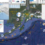
What a day. I started by waking up about 5:43 AM (about, heheh), which was 17 minutes before my alarm was set. I had a job interview at 8:30.
I went to the interview for a position working on tsunami geology. During the interview, everyone started getting phone calls and emails, there was an earthquake in Alaska. The main interviewer had to leave the interview to take a few calls. Pretty funny, before they left, they asked me what would I do. Perfect timing.
We all broke out our phones and started reviewing the early reports and hypothesizing. I thought this may be related to the earthquake in 2016, though that was much deeper.
Much has been written about this earthquake and I include tweets to summaries below in the social media section.
Today’s earthquake occurred along the convergent plate boundary in southern Alaska. This subduction zone fault is famous for the 1964 March 27 M = 9.2 megathrust earthquake. I describe this earthquake in more detail here.
During the 1964 earthquake, the downgoing Pacific plate slipped past the North America plate, including slip on “splay faults” (like the Patton fault, no relation, heheh). There was deformation along the seafloor that caused a transoceanic tsunami.
The Pacific plate has pre-existing zones of weakness related to fracture zones and spreading ridges where the plate formed and are offset. There was an earthquake in January 2016 that may have reactivated one of these fracture zones. This earthquake (M = 7.1) was very deep (~130 km), but still caused widespread damage.
There was also an earthquake associated with the faults in the Pacific plate, which is still having asftershocks, earlier this year. Here is my earthquake report for the 2018.01.24 M 7.9 earthquake. I prepared two update reports here and here.
Today’s earthquake was not on the megathrust fault interface and is extensional. I always have fun chatting with people new to subduction zones when we get to see an extensional earthquake at a convergent plate boundary. Because the earthquake was a normal earthquake (extensional) and it was rather deep, the possibility of a tsunami was quite small. However, there was a possibility that landslides could have triggered tsunami. However, these would be localized near the epicentral region.
The earthquake appears to have a depth of ~40 km and the USGS model for the megathrust fault (slab 2.0) shows the megathrust to be shallower than this earthquake. There are generally 2 ways that may explain the extensional earthquake: slab tension (the downgoing plate is pulling down on the slab, causing extension) or “bending moment” extension (as the plate bends downward, the top of the plate stretches out.

UPDATE – 1 year later

Further down on this page, I include additional materials that were developed in the past year.

Below is my interpretive poster for this earthquake

I plot the seismicity from the past month, with color representing depth and diameter representing magnitude (see legend). I include earthquake epicenters from 1918-2018 with magnitudes M ≥ 3.0 in one version.
I plot the USGS fault plane solutions (moment tensors in blue and focal mechanisms in orange), possibly in addition to some relevant historic earthquakes.

  • I placed a moment tensor / focal mechanism legend on the poster. There is more material from the USGS web sites about moment tensors and focal mechanisms (the beach ball symbols). Both moment tensors and focal mechanisms are solutions to seismologic data that reveal two possible interpretations for fault orientation and sense of motion. One must use other information, like the regional tectonics, to interpret which of the two possibilities is more likely.
  • I also include the shaking intensity contours on the map. These use the Modified Mercalli Intensity Scale (MMI; see the legend on the map). This is based upon a computer model estimate of ground motions, different from the “Did You Feel It?” estimate of ground motions that is actually based on real observations. The MMI is a qualitative measure of shaking intensity. More on the MMI scale can be found here and here. This is based upon a computer model estimate of ground motions, different from the “Did You Feel It?” estimate of ground motions that is actually based on real observations.
  • I include the slab 2.0 contours plotted (Hayes, 2018), which are contours that represent the depth to the subduction zone fault. These are mostly based upon seismicity. The depths of the earthquakes have considerable error and do not all occur along the subduction zone faults, so these slab contours are simply the best estimate for the location of the fault.li>

    Magnetic Anomalies

  • In the map below, I include a transparent overlay of the magnetic anomaly data from EMAG2 (Meyer et al., 2017). As oceanic crust is formed, it inherits the magnetic field at the time. At different points through time, the magnetic polarity (north vs. south) flips, the north pole becomes the south pole. These changes in polarity can be seen when measuring the magnetic field above oceanic plates. This is one of the fundamental evidences for plate spreading at oceanic spreading ridges (like the Gorda rise).
  • Regions with magnetic fields aligned like today’s magnetic polarity are colored red in the EMAG2 data, while reversed polarity regions are colored blue. Regions of intermediate magnetic field are colored light purple.
  • We can see the roughly east-west trends of these red and blue stripes. These lines are parallel to the ocean spreading ridges from where they were formed. The stripes disappear at the subduction zone because the oceanic crust with these anomalies is diving deep beneath the North America plate, so the magnetic anomalies from the overlying North America plate mask the evidence for the Pacific plate.

    I include some inset figures. Some of the same figures are located in different places on the larger scale map below.

  • In the upper left corner is a map of the plate boundary faults from IRIS, which shows seismicity with color representing depth. I place a blue star in the general location of today’s earthquake (same for other inset figures).
  • Below this map is a low-angle oblique view of the subduction zone.
  • In the lower right corner is a map that shows the isochrons (line of equal age) for the oceanic crust of the Pacific plate (Naugler and Wageman, 1973). Compare these lines with the magnetic anomalies in the main poster.
  • In the upper right corner is the USGS liquefaction susceptibility map which is now a standard map product for USGS earthquake pages (for earthquakes of sufficient size). There has been photos of road damage that appear to be the result of liquefaction induced slope failures. I presented this map product in my reports for the 2018.09.28 Sulawesi, Indonesia earthquake and tsunami.
  • Another new product from the USGS is an aftershock forecast. GNS (New Zealand) has been doing this for a while (I first noticed these following the 2016 Kaikoura earthquake). I prepared a table from their data that lists the potential number of earthquakes for different magnitudes for different time periods. These estimates are basically based on the empirical evidence that aftershock size and number decay with time.
  • Here is the map with a century’s seismicity plotted.

Other Report Pages

Some Relevant Discussion and Figures

  • Here is a map for the earthquakes of magnitude greater than or equal to M 7.0 between 1900 and 2016. This is the USGS query that I used to make this map. One may locate the USGS web pages for all the earthquakes on this map by following that link.

  • Here is a cross section showing the differences of vertical deformation between the coseismic (during the earthquake) and interseismic (between earthquakes).

  • Here is a figure recently published in the 5th International Conference of IGCP 588 by the Division of Geological and Geophysical Surveys, Dept. of Natural Resources, State of Alaska (State of Alaska, 2015). This is derived from a figure published originally by Plafker (1969). There is a cross section included that shows how the slip was distributed along upper plate faults (e.g. the Patton Bay and Middleton Island faults).

Below is an educational video from the USGS that presents material about subduction zones and the 1964 earthquake and tsunami in particular.
Youtube Source IRIS
mp4 file for downloading.

    Credits:

  • Animation & graphics by Jenda Johnson, geologist
  • Directed by Robert F. Butler, University of Portland
  • U.S. Geological Survey consultants: Robert C. Witter, Alaska Science Center Peter J. Haeussler, Alaska Science Center
  • Narrated by Roger Groom, Mount Tabor Middle School

    Earthquake Triggered Landslides

  • There are many different ways in which a landslide can be triggered. The first order relations behind slope failure (landslides) is that the “resisting” forces that are preventing slope failure (e.g. the strength of the bedrock or soil) are overcome by the “driving” forces that are pushing this land downwards (e.g. gravity). The ratio of resisting forces to driving forces is called the Factor of Safety (FOS). We can write this ratio like this:

    FOS = Resisting Force / Driving Force

  • When FOS > 1, the slope is stable and when FOS < 1, the slope fails and we get a landslide. The illustration below shows these relations. Note how the slope angle α can take part in this ratio (the steeper the slope, the greater impact of the mass of the slope can contribute to driving forces). The real world is more complicated than the simplified illustration below.

  • Landslide ground shaking can change the Factor of Safety in several ways that might increase the driving force or decrease the resisting force. Keefer (1984) studied a global data set of earthquake triggered landslides and found that larger earthquakes trigger larger and more numerous landslides across a larger area than do smaller earthquakes. Earthquakes can cause landslides because the seismic waves can cause the driving force to increase (the earthquake motions can “push” the land downwards), leading to a landslide. In addition, ground shaking can change the strength of these earth materials (a form of resisting force) with a process called liquefaction.
  • Sediment or soil strength is based upon the ability for sediment particles to push against each other without moving. This is a combination of friction and the forces exerted between these particles. This is loosely what we call the “angle of internal friction.” Liquefaction is a process by which pore pressure increases cause water to push out against the sediment particles so that they are no longer touching.
  • An analogy that some may be familiar with relates to a visit to the beach. When one is walking on the wet sand near the shoreline, the sand may hold the weight of our body generally pretty well. However, if we stop and vibrate our feet back and forth, this causes pore pressure to increase and we sink into the sand as the sand liquefies. Or, at least our feet sink into the sand.
  • Below is a diagram showing how an increase in pore pressure can push against the sediment particles so that they are not touching any more. This allows the particles to move around and this is why our feet sink in the sand in the analogy above. This is also what changes the strength of earth materials such that a landslide can be triggered.

  • Below is a diagram based upon a publication designed to educate the public about landslides and the processes that trigger them (USGS, 2004). Additional background information about landslide types can be found in Highland et al. (2008). There was a variety of landslide types that can be observed surrounding the earthquake region. So, this illustration can help people when they observing the landscape response to the earthquake whether they are using aerial imagery, photos in newspaper or website articles, or videos on social media. Will you be able to locate a landslide scarp or the toe of a landslide? This figure shows a rotational landslide, one where the land rotates along a curvilinear failure surface.

  • Here is an excellent educational video from IRIS and a variety of organizations. The video helps us learn about how earthquake intensity gets smaller with distance from an earthquake. The concept of liquefaction is reviewed and we learn how different types of bedrock and underlying earth materials can affect the severity of ground shaking in a given location. The intensity map above is based on a model that relates intensity with distance to the earthquake, but does not incorporate changes in material properties as the video below mentions is an important factor that can increase intensity in places.
  • If we look at the map at the top of this report, we might imagine that because the areas close to the fault shake more strongly, there may be more landslides in those areas. This is probably true at first order, but the variation in material properties and water content also control where landslides might occur.
  • There are landslide slope stability and liquefaction susceptibility models based on empirical data from past earthquakes. The USGS has recently incorporated these types of analyses into their earthquake event pages. More about these USGS models can be found on this page.
  • Here is the USGS liquefaction susceptibility map. Learn more about the background behind this map here.

UPDATE – 1 year later 2019.11.30

Well, I now have the job that I was being interviewed for one year ago today.
Head over to the University of Alaska Fairbanks, Alaska Earthquake Center, to see a one year review of this earthquake sequence (which is still having aftershocks).
The USGS Alaska Science Center also has an excellent review of this earthquake sequence here.
Some of the material in this update came from the days immediately following the earthquake, but did not get into the Earthquake Report.
There was an Earthquake Symposium about this earthquake sequence earlier this year. Head over there to see the presentations from that symposium.

  • Here is a figure from the Alaska Earthquake Center that shows seismograms from the Anchorage area.

  • Here is a map from Dr. Eric Fielding (NASA/JPL-Caltech) that uses Copernicus Sentinel satellite based RADAR data. The process is called interferometric RADAR (InSAR) analysis.

  • Here is the Global Positioning System (GPS) analysis done by Dr. Bill Hammond from the Nevada Geodetic Laboratory. The red arrows (vectors, which show direction and magnitude) represent the motion at the GPS sites that happened during the earthquake (the “coseismic” motion). There is a scale in the lower right corner. The ellipses at the end of the arrow represent the uncertainty (error) for those measurements. The GPS sites are at the base of the arrow (the opposite end from the arrowhead).

Geologic Fundamentals

  • For more on the graphical representation of moment tensors and focal mechnisms, check this IRIS video out:
  • Here is a fantastic infographic from Frisch et al. (2011). This figure shows some examples of earthquakes in different plate tectonic settings, and what their fault plane solutions are. There is a cross section showing these focal mechanisms for a thrust or reverse earthquake. The upper right corner includes my favorite figure of all time. This shows the first motion (up or down) for each of the four quadrants. This figure also shows how the amplitude of the seismic waves are greatest (generally) in the middle of the quadrant and decrease to zero at the nodal planes (the boundary of each quadrant).

  • Here is another way to look at these beach balls.
  • There are three types of earthquakes, strike-slip, compressional (reverse or thrust, depending upon the dip of the fault), and extensional (normal). Here is are some animations of these three types of earthquake faults. The following three animations are from IRIS.
  • Strike Slip:

    Compressional:

    Extensional:

  • This is an image from the USGS that shows how, when an oceanic plate moves over a hotspot, the volcanoes formed over the hotspot form a series of volcanoes that increase in age in the direction of plate motion. The presumption is that the hotspot is stable and stays in one location. Torsvik et al. (2017) use various methods to evaluate why this is a false presumption for the Hawaii Hotspot.

  • A cutaway view along the Hawaiian island chain showing the inferred mantle plume that has fed the Hawaiian hot spot on the overriding Pacific Plate. The geologic ages of the oldest volcano on each island (Ma = millions of years ago) are progressively older to the northwest, consistent with the hot spot model for the origin of the Hawaiian Ridge-Emperor Seamount Chain. (Modified from image of Joel E. Robinson, USGS, in “This Dynamic Planet” map of Simkin and others, 2006.)

  • Here is a map from Torsvik et al. (2017) that shows the age of volcanic rocks at different locations along the Hawaii-Emperor Seamount Chain.

  • Hawaiian-Emperor Chain. White dots are the locations of radiometrically dated seamounts, atolls and islands, based on compilations of Doubrovine et al. and O’Connor et al. Features encircled with larger white circles are discussed in the text and Fig. 2. Marine gravity anomaly map is from Sandwell and Smith.

Return to the Earthquake Reports page.


Earthquake Report: Blanco fracture zone

Well, so exciting to have more earthquakes to write about! This summer has been a low seismic summer. The entire year actually.
There was an earthquake within the Gorda plate a few days ago, but these M 5.3 and M 5.6 earthquakes are unlikely to be related, at least in a physical reality sort of way. Here is my Earthquake Report for the Gorda plate earthquake sequence.
This morning (my time) there was an earthquake along the Blanco fracture zone system (BFZ). Today’s earthquake(s) are too small and too far away to directly affect or impact the Cascadia subduction zone megathrust fault. However, I prepare this report because it is a great way to explore the complexities along the BFZ.
The BFZ is a transform plate boundary that connects the Juan de Fuca ridge with the Gorda rise spreading centers. This active fault zone consists of numerous right-lateral (dextral) faults. There is some debate as to how far east the BFZ extends beyond the Gorda rise (some pose it extends far past the trench and ambient noise tomographic data supports this interpretation; Porritt et al., 2011). I remember a colleague of mine who once adamantly stated that there is no evidence for the extension of the BFZ eastwards past the megathrust fault tip. However, this colleague made this statement a decade before the Porritt et al. (2011) data were to be published. My colleague is may still be correct as other experts agree with them.
The interesting thing about today’s M 5.3 earthquake is that it is extensional (normal faulting). This is not altogether unexpected, but interesting nonetheless. Most people might expect the BFZ to have dominantly strike-slip earthquakes. This is largely true, but there are “pull-apart basins” along the BFZ. As strike-slip faults may not be oriented perfectly to the strain field (the tectonic forces driving plate motion and deformation of the lithosphere or crust), other structures may form to accommodate this imperfection. One example of this is a pull apart basin. There are various other causes for pull apart basins too. For example, as faults may bend or change orientation (also in response to the strain field), pull apart basins (or compressional pop up structures) may form.
However, it is possible (probable, given the bathymetric data) that this M 5.3 is not associated with a pull apart basin, but simply the reactivation of a spreading ridge normal fault in response to the complicated tectonics along the BFZ.

Magnetic Anomalies

  • In the map below, I include a transparent overlay of the magnetic anomaly data from EMAG2 (Meyer et al., 2017). As oceanic crust is formed, it inherits the magnetic field at the time. At different points through time, the magnetic polarity (north vs. south) flips, the north pole becomes the south pole. These changes in polarity can be seen when measuring the magnetic field above oceanic plates. This is one of the fundamental evidences for plate spreading at oceanic spreading ridges (like the Gorda rise).
  • Regions with magnetic fields aligned like today’s magnetic polarity are colored red in the EMAG2 data, while reversed polarity regions are colored blue. Regions of intermediate magnetic field are colored light purple.
  • Note that along the Gorda rise, the magnetic anomaly is red, showing that the spreading ridge has a normal polarity, like that of today. Prior to about 780,000 years ago, the polarity was reversed. During the Bruhnes-Matuyama magnetic polarity reversal, the polarity flipped to the way it is today. Note how as one goes away from the Gorda rise (east or west), the magnetic anomaly changes color to blue. At the boundary between red and blue is the Bruhnes-Matuyama magnetic polarity reversal.
  • The structures in the Gorda, Juad de Fuca, and Pacific plates in this region are largely inherited from the extensional tectonic and volcanic processes at the Gorda rise and Juan de Fuca Ridge. However, the Gorda plate is being pulverized by the surrounding tectonic plates. There are several interpretations about how the plate is deforming and some debate about whether the Gorda plate is even behaving like a plate.
  • Note how some of the magnetic anomalies appear to be offset along lines that are sub-parallel to the BFZ. This is because they are.

Below is my interpretive poster for this earthquake

I plot the seismicity from the past month, with color representing depth and diameter representing magnitude (see legend). I one version, I include earthquake epicenters from 1918-2018 with magnitudes M ≥ 6.0.
I plot the USGS fault plane solutions (moment tensors in blue and focal mechanisms in orange), possibly in addition to some relevant historic earthquakes.

  • I placed a moment tensor / focal mechanism legend on the poster. There is more material from the USGS web sites about moment tensors and focal mechanisms (the beach ball symbols). Both moment tensors and focal mechanisms are solutions to seismologic data that reveal two possible interpretations for fault orientation and sense of motion. One must use other information, like the regional tectonics, to interpret which of the two possibilities is more likely.
  • I include some inset figures.

  • In the upper right corner is a map of the Cascadia subduction zone (CSZ) and regional tectonic plate boundary faults. This is modified from several sources (Chaytor et al., 2004; Nelson et al., 2004). I placed a blue stars in the general location of today’s earthquake (as in other inset figures in this poster).
  • In the lower right corner is an illustration modified from Plafker (1972). This figure shows how a subduction zone deforms between (interseismic) and during (coseismic) earthquakes. Today’s earthquake did not occur along the CSZ, so did not produce crustal deformation like this. However, it is useful to know this when studying the CSZ. Today’s earthquakes happened in the lower Gorda plate
  • In the upper left corner is a map showing the details for the faulting along the BFZ (Braunmiller and Nabelek (2008). Note that this zone is quite complicated and includes several nornal fault bounded pull-apart basins.
  • In the lower left corner is a map from Dziak et al. (2000) that shows the topography (in the upper panel) and the faulting (in the lower panel) along the BFZ. Blue = lower elevation, deeper oceanic depths; Red = shallower oceanic depth, higher elevation. I placed orange arrows to help one locate the normal faults (perpendicular to the strike-slip faults) in this map. Compare this inset map with the Google Earth bathymetry in the main map. Can you see the BFZ perpendicular ridges?

USGS Earthquake Pages

    These are from this current sequence

  • 2018-07-29 M 5.3
  • Here is the map with the seismicity from the past 30 days.

  • Here is the same map with the seismicity from 1918-2018.

Some Relevant Discussion and Figures

  • Here is a map of the Cascadia subduction zone, modified from Nelson et al. (2006). The Juan de Fuca and Gorda plates subduct norteastwardly beneath the North America plate at rates ranging from 29- to 45-mm/yr. Sites where evidence of past earthquakes (paleoseismology) are denoted by white dots. Where there is also evidence for past CSZ tsunami, there are black dots. These paleoseismology sites are labeled (e.g. Humboldt Bay). Some submarine paleoseismology core sites are also shown as grey dots. The two main spreading ridges are not labeled, but the northern one is the Juan de Fuca ridge (where oceanic crust is formed for the Juan de Fuca plate) and the southern one is the Gorda rise (where the oceanic crust is formed for the Gorda plate).

  • Here is a version of the CSZ cross section alone (Plafker, 1972). This shows two parts of the earthquake cycle: the interseismic part (between earthquakes) and the coseismic part (during earthquakes). Regions that experience uplift during the interseismic period tend to experience subsidence during the coseismic period.

  • This is a diagram that shows how a pull apart basin might form (Wu et al., 2009).

  • General characteristics of a pull-apart basin in a dextral side-stepping fault system. The pull-apart basin is defined to develop in pure strike-slip when alpha = 0 degrees and in transtension when 0 degrees < alpha 45 degrees.

  • This figure shows the results of modeling in clay, showing a pull apart basin form (Wu et al., 2009).

  • Plan view evolution of transtensional pull-apart basin model illustrated with: (a) time-lapse overhead photography; and (b) fault interpretation and incremental basin subsidence calculated from differential laser scans. Initial and final baseplate geometry shown with dashed lines; (c) basin topography at end of experiment.

  • With these analog models in mind, consider the map below from Braunmiller and Nabelek (2008). This map shows bathymetry (depth in the ocean) in color (units in meters below sea level). They also plot earthquake mechanisms to show how there is extension at the boundary of these basins and strike-slip motion along the strike slip faults. The uncertainty in their locaions are represented by the crosses. I include their figure caption below

  • Close-up of the BTFZ. Plotted are fault plane solutions (gray scheme as in Figure 10) and well-relocated earthquake epicenters. SeaBeam data are from the RIDGE Multibeam Synthesis Project (http://imager.ldeo.columbia.edu) at the Lamont-Doherty Earth Observatory. Solid and dashed lines mark inferred [Embley and Wilson, 1992] locations of active
    and inactive faults, respectively.

  • Here is a detailed map showing a pull apart basin just to the southwest of today’s M 5.3 (Braunmiller and Nabelek, 2008). I include their figure caption below.

  • Close-up of the BTFZ-Juan de Fuca ridge-transform intersection. The deep basins are East Blanco Depression (EBD) and West Blanco Depression (WBD); the bathymetric high south of WBD is the Parks Plateau. White arrows are slip vector azimuths of strike-slip events (Figure 16) with tails at their epicenters. Possible active fault strands are shown schematically as solid and dashed lines and are marked (WBDN, WBDC, WBDS, and PPF); solid northerly trending lines illustrate right stepping of (some) transform motion at the EBD.

  • This is the figure from Dziak et al. (2000) for us to evaluate. I include their long figure caption below.

  • (Top) Sea Beam bathymetric map of the Cascadia Depression, Blanco Ridge, and Gorda Depression, eastern Blanco Transform Fault Zone (BTFZ).Multibeam bathymetry was collected by the NOAA R/V’s Surveyor and Discoverer and the R/V Laney Chouest during 12 cruises in the 1980’s and 90’s. Bathymetry displayed using a 500 m grid interval. Numbers with arrows show look directions of three-dimensional diagrams in Figures 2 and 3. (Bottom) Structure map, interpreted from bathymetry, showing active faults and major geologic features of the region. Solid lines represent faults, dashed lines are fracture zones, and dotted lines show course of turbidite channels. When possible to estimate sense of motion on a fault, a filled circle shows the down-thrown side. Inset maps show location and generalized geologic structure of the BTFZ. Location of seismic reflection and gravity/magnetics profiles indicated by opposing brackets. D-D’ and E-E’ are the seismic reflection profiles shown in Figures 8a and 8b, and G-G’ is the gravity and magnetics profile shown in Figure 13. Submersible dive tracklines from sites 1 through 4 are highlighted in red. L1 and L2 are two lineations seen in three-dimensional bathymetry shown in Figures 2 and 3. Location of two Blanco Ridge slump scars indicated by half-rectangles, inferred direction of slump shown by arrow, and debris location (when identified) designated by an ‘S’. CD stands for Cascadia Depression, BR is Blanco Ridge, GD is Gorda Depression, and GR is Gorda Ridge. Numbers on north and south side of transform represent Juan de Fuca and Pacific plate crustal ages inferred from magnetic anomalies. Long-term plate motion rate between the Pacific and southern Juan de Fuca plates from Wilson (1989).

BFZ Historic Seismicity

  • There were two Mw 4.2 earthquakes associated with this plate boundary fault system in mid 2015. I plot the moment tensors for these earthquakes (USGS pages: 4/7/15 and 4/11/15) in this map below. I also have placed the relative plate motions as arrows, labeled the plates, and placed a transparent focal mechanism plot above the BFZ showing the general sense of motion across this plate boundary. There have been several earthquakes along the Mendocino fault recently and I write about them 1/2015 here and 4/2015 here.

  • There was also seismic activity along the BFZ later in 2015. Here are my report and report update.
  • Here is a map showing these earthquakes, with moment tensors plotted for the M 5.8 and M 5.5 earthquakes. I include an inset map showing the plate configuration based upon the Nelson et al. (2004) and Chaytor et al. (2004) papers (I modified it). I also include a cross section of the subduction zone, as it is configured in-between earthquakes (interseismic) and during earthquakes (coseismic), modified from Plafker (1972).

  • I put together an animation that includes the seismicity from 1/1/2000 until 6/1/2015 for the region near the Blanco fracture zone, with earthquake magnitudes greater than or equal to M = 5.0. The map here shows all these epicenters, with the moment tensors for earthquakes of M = 6 or more (plus the two largest earthquakes from today’s swarm). Here is the page that I posted regarding the beginning of this swarm. Here is a post from some earthquakes earlier this year along the BFZ.
  • Earthquake epicenters are plotted with the depth designated by color and the magnitude depicted by the size of the circle. These are all fairly shallow earthquakes at depths suitable for oceanic lithosphere.

    Here is the list of the earthquakes with moment tensors plotted in the above maps (with links to the USGS websites for those earthquakes):

  • 2000/06/02 M 6.0
  • 2003/01/16 M 6.3
  • 2008/01/10 M 6.3
  • 2012/04/12 M 6.0
  • 2015/06/01 M 5.8
  • 2015/06/01 M 5.9
    Here are some files that are outputs from that USGS search above.

  • csv file
  • kml file (not animated)
  • kml file (animated)

VIDEOS

    Here are links to the video files (it might be easier to download them and view them remotely as the files are large).

  • First Animation (20 mb mp4 file)
  • Second Animation (10 mb mp4 file)

Here is the first animation that first adds the epicenters through time (beginning with the oldest earthquakes), then removes them through time (beginning with the oldest earthquakes).


Here is the second animation that uses a one-year moving window. This way, one year after an earthquake is plotted, it is removed from the plot. This animation is good to see the spatiotemporal variation of seismicity along the BFZ.

Here is a map with all the fore- and after-shocks plotted to date.

Geologic Fundamentals

  • For more on the graphical representation of moment tensors and focal mechnisms, check this IRIS video out:
  • Here is a fantastic infographic from Frisch et al. (2011). This figure shows some examples of earthquakes in different plate tectonic settings, and what their fault plane solutions are. There is a cross section showing these focal mechanisms for a thrust or reverse earthquake. The upper right corner includes my favorite figure of all time. This shows the first motion (up or down) for each of the four quadrants. This figure also shows how the amplitude of the seismic waves are greatest (generally) in the middle of the quadrant and decrease to zero at the nodal planes (the boundary of each quadrant).

  • There are three types of earthquakes, strike-slip, compressional (reverse or thrust, depending upon the dip of the fault), and extensional (normal). Here is are some animations of these three types of earthquake faults. The following three animations are from IRIS.
  • Strike Slip:

    Compressional:

    Extensional:

  • This is an image from the USGS that shows how, when an oceanic plate moves over a hotspot, the volcanoes formed over the hotspot form a series of volcanoes that increase in age in the direction of plate motion. The presumption is that the hotspot is stable and stays in one location. Torsvik et al. (2017) use various methods to evaluate why this is a false presumption for the Hawaii Hotspot.

  • A cutaway view along the Hawaiian island chain showing the inferred mantle plume that has fed the Hawaiian hot spot on the overriding Pacific Plate. The geologic ages of the oldest volcano on each island (Ma = millions of years ago) are progressively older to the northwest, consistent with the hot spot model for the origin of the Hawaiian Ridge-Emperor Seamount Chain. (Modified from image of Joel E. Robinson, USGS, in “This Dynamic Planet” map of Simkin and others, 2006.)

  • Here is a map from Torsvik et al. (2017) that shows the age of volcanic rocks at different locations along the Hawaii-Emperor Seamount Chain.

  • Hawaiian-Emperor Chain. White dots are the locations of radiometrically dated seamounts, atolls and islands, based on compilations of Doubrovine et al. and O’Connor et al. Features encircled with larger white circles are discussed in the text and Fig. 2. Marine gravity anomaly map is from Sandwell and Smith.


    Social Media

    References:

  • Atwater, B.F., Musumi-Rokkaku, S., Satake, K., Tsuju, Y., Eueda, K., and Yamaguchi, D.K., 2005. The Orphan Tsunami of 1700—Japanese Clues to a Parent Earthquake in North America, USGS Professional Paper 1707, USGS, Reston, VA, 144 pp.
  • Chaytor, J.D., Goldfinger, C., Dziak, R.P., and Fox, C.G., 2004. Active deformation of the Gorda plate: Constraining deformation models with new geophysical data: Geology v. 32, p. 353-356.
  • Dengler, L.A., Moley, K.M., McPherson, R.C., Pasyanos, M., Dewey, J.W., and Murray, M., 1995. The September 1, 1994 Mendocino Fault Earthquake, California Geology, Marc/April 1995, p. 43-53.
  • Dziak, R.P., Fox, C.G., Embleey, R.W., Nabelek, J.L., Braunmiller, J., and Koski, R.A., 2000. Recent tectonics of the Blanco Ridge, eastern blanco transform fault zone in Marine Geophysical Researches, vol. 21, p. 423-450
  • Frisch, W., Meschede, M., Blakey, R., 2011. Plate Tectonics, Springer-Verlag, London, 213 pp.
  • Geist, E.L. and Andrews D.J., 2000. Slip rates on San Francisco Bay area faults from anelastic deformation of the continental lithosphere, Journal of Geophysical Research, v. 105, no. B11, p. 25,543-25,552.
  • Irwin, W.P., 1990. Quaternary deformation, in Wallace, R.E. (ed.), 1990, The San Andreas Fault system, California: U.S. Geological Survey Professional Paper 1515, online at: http://pubs.usgs.gov/pp/1990/1515/
  • Lin, J., R. S. Stein, M. Meghraoui, S. Toda, A. Ayadi, C. Dorbath, and S. Belabbes (2011), Stress transfer among en echelon and opposing thrusts and tear faults: Triggering caused by the 2003 Mw = 6.9 Zemmouri, Algeria, earthquake, J. Geophys. Res., 116, B03305, doi:10.1029/2010JB007654.
  • McCrory, P.A.,. Blair, J.L., Waldhauser, F., kand Oppenheimer, D.H., 2012. Juan de Fuca slab geometry and its relation to Wadati-Benioff zone seismicity in JGR, v. 117, B09306, doi:10.1029/2012JB009407.
  • McLaughlin, R.J., Sarna-Wojcicki, A.M., Wagner, D.L., Fleck, R.J., Langenheim, V.E., Jachens, R.C., Clahan, K., and Allen, J.R., 2012. Evolution of the Rodgers Creek–Maacama right-lateral fault system and associated basins east of the northward-migrating Mendocino Triple Junction, northern California in Geosphere, v. 8, no. 2., p. 342-373.
  • Meyer, B., Saltus, R., Chulliat, a., 2017. EMAG2: Earth Magnetic Anomaly Grid (2-arc-minute resolution) Version 3. National Centers for Environmental Information, NOAA. Model. doi:10.7289/V5H70CVX
  • Nelson, A.R., Asquith, A.C., and Grant, W.C., 2004. Great Earthquakes and Tsunamis of the Past 2000 Years at the Salmon River Estuary, Central Oregon Coast, USA: Bulletin of the Seismological Society of America, Vol. 94, No. 4, pp. 1276–1292
  • Rollins, J.C. and Stein, R.S., 2010. Coulomb stress interactions among M ≥ 5.9 earthquakes in the Gorda deformation zone and on the Mendocino Fault Zone, Cascadia subduction zone, and northern San Andreas Fault: Journal of Geophysical Research, v. 115, B12306, doi:10.1029/2009JB007117, 2010.
  • Stoffer, P.W., 2006, Where’s the San Andreas Fault? A guidebook to tracing the fault on public lands in the San Francisco Bay region: U.S. Geological Survey General Interest Publication 16, 123 p., online at http://pubs.usgs.gov/gip/2006/16/
  • Yue, H., Zhang, Z., Chen, Y.J., 2008. Interaction between adjacent left-lateral strike-slip faults and thrust faults: the 1976 Songpan earthquake sequence in Chinese Science Bulletin, v. 53, no. 16, p. 2520-2526
  • Wallace, Robert E., ed., 1990, The San Andreas fault system, California: U.S. Geological Survey Professional Paper 1515, 283 p. [http://pubs.usgs.gov/pp/1988/1434/].

°

#Earthquake Report: Gorda plate

Over the past night and morning, there was a sequence of earthquakes within the Gorda plate due west of Crescent City. Some people even felt these earthquakes, culminating (so far) with a M 5.6. There was a Gorda plate earthquake in March of this year, but it was in a different location.
These earthquakes did not occur along the Gorda Rise as some have reported, but within a region of oceanic crust over a million years old.
In the map below, I include a transparent overlay of the magnetic anomaly data from EMAG2 (Meyer et al., 2017). As oceanic crust is formed, it inherits the magnetic field at the time. At different points through time, the magnetic polarity (north vs. south) flips, the north pole becomes the south pole. These changes in polarity can be seen when measuring the magnetic field above oceanic plates. This is one of the fundamental evidences for plate spreading at oceanic spreading ridges (like the Gorda rise).
Regions with magnetic fields aligned like today’s magnetic polarity are colored red in the EMAG2 data, while reversed polarity regions are colored blue. Regions of intermediate magnetic field are colored light purple.
Note that along the Gorda rise, the magnetic anomaly is red, showing that the spreading ridge has a normal polarity, like that of today. Prior to about 780,000 years ago, the polarity was reversed. During the Bruhnes-Matuyama magnetic polarity reversal, the polarity flipped to the way it is today. Note how as one goes away from the Gorda rise (east or west), the magnetic anomaly changes color to blue. At the boundary between red and blue is the Bruhnes-Matuyama magnetic polarity reversal. The earthquakes from today occurred within this blue region, so the oceanic crust is older than about 780,000 years old, probably older than a million years old.
The structures in the Gorda plate in this region are largely inherited from the extensional tectonic and volcanic processes at the Gorda rise. However, the Gorda plate is being pulverized by the surrounding tectonic plates. There are several interpretations about how the plate is deforming and some debate about whether the Gorda plate is even behaving like a plate. These normal fault (extensional) structures have been reactivating as left-lateral strike-slip faults as a result of this deformation. This region is called the Mendocino deformation zone (a.k.a. the Triangle of Doom).

Below is my interpretive poster for this earthquake

I plot the seismicity from the past month, with color representing depth and diameter representing magnitude (see legend). I include earthquake epicenters from 1918-2018 with magnitudes M ≥ 5.0 in a second poster).
I plot the USGS fault plane solutions (moment tensors in blue and focal mechanisms in orange), in addition to some relevant historic earthquakes.

  • I placed a moment tensor / focal mechanism legend on the poster. There is more material from the USGS web sites about moment tensors and focal mechanisms (the beach ball symbols). Both moment tensors and focal mechanisms are solutions to seismologic data that reveal two possible interpretations for fault orientation and sense of motion. One must use other information, like the regional tectonics, to interpret which of the two possibilities is more likely.
  • I include some inset figures.

  • In the upper right corner is a map of the Cascadia subduction zone (CSZ) and regional tectonic plate boundary faults. This is modified from several sources (Chaytor et al., 2004; Nelson et al., 2004). I placed a blue stars in the general location of today’s earthquakes.
  • In the upper left corner is a map from Chaytor et al. (2004) that shows some details of the faulting in the region. This figure shows the predominant tectonic fabric in the GP (northeast striking left-lateral faults). More about this figure can be found below.
  • In the lower right corner is a figure from Rollins and Stein (2010). In their paper they discuss how static coulomb stress changes from earthquakes may impart (or remove) stress from adjacent crust/faults. I place a blues star in the general location of today’s earthquakes.
  • In the lower left corner is a figure from Chaytor et al. (2004) that shows the different models for the internal deformation within the Gorda plate.


  • This version includes earthquakes M ≥ 5.0 from the USGS. Note how the region where today’s earthquakes happened is a region of higher levels of seismicity. Perhaps this is because this region is the locus of the deformation within the Mendocino deformation zone?


USGS Earthquake Pages

  • However, this region is typified by these normal (extensional earthquakes. Below are some of these.
  • 1985.07.23 M 5.3
  • 1990.01.05 M 5.4
  • 2013.12.01 M 5.5

Some Relevant Discussion and Figures

  • Here is a map of the Cascadia subduction zone, modified from Nelson et al. (2006). The Juan de Fuca and Gorda plates subduct norteastwardly beneath the North America plate at rates ranging from 29- to 45-mm/yr. Sites where evidence of past earthquakes (paleoseismology) are denoted by white dots. Where there is also evidence for past CSZ tsunami, there are black dots. These paleoseismology sites are labeled (e.g. Humboldt Bay). Some submarine paleoseismology core sites are also shown as grey dots. The two main spreading ridges are not labeled, but the northern one is the Juan de Fuca ridge (where oceanic crust is formed for the Juan de Fuca plate) and the southern one is the Gorda rise (where the oceanic crust is formed for the Gorda plate).

  • Here is a version of the CSZ cross section alone (Plafker, 1972). This shows two parts of the earthquake cycle: the interseismic part (between earthquakes) and the coseismic part (during earthquakes). Regions that experience uplift during the interseismic period tend to experience subsidence during the coseismic period.

  • Here is a map from Chaytor et al. (2004) that shows some details of the faulting in the region. The moment tensor (at the moment i write this) shows a north-south striking fault with a reverse or thrust faulting mechanism. While this region of faulting is dominated by strike slip faults (and most all prior earthquake moment tensors showed strike slip earthquakes), when strike slip faults bend, they can create compression (transpression) and extension (transtension). This transpressive or transtentional deformation may produce thrust/reverse earthquakes or normal fault earthquakes, respectively. The transverse ranges north of Los Angeles are an example of uplift/transpression due to the bend in the San Andreas fault in that region.

  • A: Mapped faults and fault-related ridges within Gorda plate based on basement structure and surface morphology, overlain on bathymetric contours (gray lines—250 m interval). Approximate boundaries of three structural segments are also shown. Black arrows indicated approximate location of possible northwest- trending large-scale folds. B, C: uninterpreted and interpreted enlargements of center of plate showing location of interpreted second-generation strike-slip faults and features that they appear to offset. OSC—overlapping spreading center.

  • These are the models for tectonic deformation within the Gorda plate as presented by Jason Chaytor in 2004.
  • Mw = 5 Trinidad Chaytor

    Models of brittle deformation for Gorda plate overlain on magnetic anomalies modified from Raff and Mason (1961). Models A–F were proposed prior to collection and analysis of full-plate multibeam data. Deformation model of Gulick et al. (2001) is included in model A. Model G represents modification of Stoddard’s (1987) flexural-slip model proposed in this paper.

  • Here is a map from Rollins and Stein, showing their interpretations of different historic earthquakes in the region. This was published in response to the Januray 2010 Gorda plate earthquake. The faults are from Chaytor et al. (2004).

  • Tectonic configuration of the Gorda deformation zone and locations and source models for 1976–2010 M ≥ 5.9 earthquakes. Letters designate chronological order of earthquakes (Table 1 and Appendix A). Plate motion vectors relative to the Pacific Plate (gray arrows in main diagram) are from Wilson [1989], with Cande and Kent’s [1995] timescale correction.

  • In this map below, I label a number of other significant earthquakes in this Mendocino triple junction region. Another historic right-lateral earthquake on the Mendocino fault system was in 1994. There was a series of earthquakes possibly along the easternmost section of the Mendocino fault system in late January 2015, here is my post about that earthquake series.

The Gorda and Juan de Fuca plates subduct beneath the North America plate to form the Cascadia subduction zone fault system. In 1992 there was a swarm of earthquakes with the magnitude Mw 7.2 Mainshock on 4/25. Initially this earthquake was interpreted to have been on the Cascadia subduction zone (CSZ). The moment tensor shows a compressional mechanism. However the two largest aftershocks on 4/26/1992 (Mw 6.5 and Mw 6.7), had strike-slip moment tensors. These two aftershocks align on what may be the eastern extension of the Mendocino fault.
There have been several series of intra-plate earthquakes in the Gorda plate. Two main shocks that I plot of this type of earthquake are the 1980 (Mw 7.2) and 2005 (Mw 7.2) earthquakes. I place orange lines approximately where the faults are that ruptured in 1980 and 2005. These are also plotted in the Rollins and Stein (2010) figure above. The Gorda plate is being deformed due to compression between the Pacific plate to the south and the Juan de Fuca plate to the north. Due to this north-south compression, the plate is deforming internally so that normal faults that formed at the spreading center (the Gorda Rise) are reactivated as left-lateral strike-slip faults. In 2014, there was another swarm of left-lateral earthquakes in the Gorda plate. I posted some material about the Gorda plate setting on this page.

Cascadia subduction zone Earthquake Reports

General Overview

  • 1700.09.26 M 9.0 Cascadia’s 315th Anniversary 2015.01.26
  • 1700.09.26 M 9.0 Cascadia’s 316th Anniversary 2016.01.26 updated in 2017 and 2018
  • 1992.04.25 M 7.1 Cape Mendocino 25 year remembrance
  • 1992.04.25 M 7.1 Cape Mendocino 25 Year Remembrance Event Page
  • Earthquake Information about the CSZ 2015.10.08
  • Earthquake Reports

    Gorda plate

    Blanco fracture zone

    Mendocino fault

    Mendocino triple junction

    North America plate

    Explorer plate

    Uncertain

    Geologic Fundamentals

    • For more on the graphical representation of moment tensors and focal mechnisms, check this IRIS video out:
    • Here is a fantastic infographic from Frisch et al. (2011). This figure shows some examples of earthquakes in different plate tectonic settings, and what their fault plane solutions are. There is a cross section showing these focal mechanisms for a thrust or reverse earthquake. The upper right corner includes my favorite figure of all time. This shows the first motion (up or down) for each of the four quadrants. This figure also shows how the amplitude of the seismic waves are greatest (generally) in the middle of the quadrant and decrease to zero at the nodal planes (the boundary of each quadrant).

    • There are three types of earthquakes, strike-slip, compressional (reverse or thrust, depending upon the dip of the fault), and extensional (normal). Here is are some animations of these three types of earthquake faults. The following three animations are from IRIS.
    • Strike Slip:

      Compressional:

      Extensional:

    • This is an image from the USGS that shows how, when an oceanic plate moves over a hotspot, the volcanoes formed over the hotspot form a series of volcanoes that increase in age in the direction of plate motion. The presumption is that the hotspot is stable and stays in one location. Torsvik et al. (2017) use various methods to evaluate why this is a false presumption for the Hawaii Hotspot.

    • A cutaway view along the Hawaiian island chain showing the inferred mantle plume that has fed the Hawaiian hot spot on the overriding Pacific Plate. The geologic ages of the oldest volcano on each island (Ma = millions of years ago) are progressively older to the northwest, consistent with the hot spot model for the origin of the Hawaiian Ridge-Emperor Seamount Chain. (Modified from image of Joel E. Robinson, USGS, in “This Dynamic Planet” map of Simkin and others, 2006.)

    • Here is a map from Torsvik et al. (2017) that shows the age of volcanic rocks at different locations along the Hawaii-Emperor Seamount Chain.

    • Hawaiian-Emperor Chain. White dots are the locations of radiometrically dated seamounts, atolls and islands, based on compilations of Doubrovine et al. and O’Connor et al. Features encircled with larger white circles are discussed in the text and Fig. 2. Marine gravity anomaly map is from Sandwell and Smith.

    Social Media

      References:

    • Atwater, B.F., Musumi-Rokkaku, S., Satake, K., Tsuju, Y., Eueda, K., and Yamaguchi, D.K., 2005. The Orphan Tsunami of 1700—Japanese Clues to a Parent Earthquake in North America, USGS Professional Paper 1707, USGS, Reston, VA, 144 pp.
    • Chaytor, J.D., Goldfinger, C., Dziak, R.P., and Fox, C.G., 2004. Active deformation of the Gorda plate: Constraining deformation models with new geophysical data: Geology v. 32, p. 353-356.
    • Dengler, L.A., Moley, K.M., McPherson, R.C., Pasyanos, M., Dewey, J.W., and Murray, M., 1995. The September 1, 1994 Mendocino Fault Earthquake, California Geology, Marc/April 1995, p. 43-53.
    • Frisch, W., Meschede, M., Blakey, R., 2011. Plate Tectonics, Springer-Verlag, London, 213 pp.
    • Geist, E.L. and Andrews D.J., 2000. Slip rates on San Francisco Bay area faults from anelastic deformation of the continental lithosphere, Journal of Geophysical Research, v. 105, no. B11, p. 25,543-25,552.
    • Irwin, W.P., 1990. Quaternary deformation, in Wallace, R.E. (ed.), 1990, The San Andreas Fault system, California: U.S. Geological Survey Professional Paper 1515, online at: http://pubs.usgs.gov/pp/1990/1515/
    • Lin, J., R. S. Stein, M. Meghraoui, S. Toda, A. Ayadi, C. Dorbath, and S. Belabbes (2011), Stress transfer among en echelon and opposing thrusts and tear faults: Triggering caused by the 2003 Mw = 6.9 Zemmouri, Algeria, earthquake, J. Geophys. Res., 116, B03305, doi:10.1029/2010JB007654.
    • McCrory, P.A.,. Blair, J.L., Waldhauser, F., kand Oppenheimer, D.H., 2012. Juan de Fuca slab geometry and its relation to Wadati-Benioff zone seismicity in JGR, v. 117, B09306, doi:10.1029/2012JB009407.
    • McLaughlin, R.J., Sarna-Wojcicki, A.M., Wagner, D.L., Fleck, R.J., Langenheim, V.E., Jachens, R.C., Clahan, K., and Allen, J.R., 2012. Evolution of the Rodgers Creek–Maacama right-lateral fault system and associated basins east of the northward-migrating Mendocino Triple Junction, northern California in Geosphere, v. 8, no. 2., p. 342-373.
    • Meyer, B., Saltus, R., Chulliat, a., 2017. EMAG2: Earth Magnetic Anomaly Grid (2-arc-minute resolution) Version 3. National Centers for Environmental Information, NOAA. Model. doi:10.7289/V5H70CVX
    • Nelson, A.R., Asquith, A.C., and Grant, W.C., 2004. Great Earthquakes and Tsunamis of the Past 2000 Years at the Salmon River Estuary, Central Oregon Coast, USA: Bulletin of the Seismological Society of America, Vol. 94, No. 4, pp. 1276–1292
    • Rollins, J.C. and Stein, R.S., 2010. Coulomb stress interactions among M ≥ 5.9 earthquakes in the Gorda deformation zone and on the Mendocino Fault Zone, Cascadia subduction zone, and northern San Andreas Fault: Journal of Geophysical Research, v. 115, B12306, doi:10.1029/2009JB007117, 2010.
    • Stoffer, P.W., 2006, Where’s the San Andreas Fault? A guidebook to tracing the fault on public lands in the San Francisco Bay region: U.S. Geological Survey General Interest Publication 16, 123 p., online at http://pubs.usgs.gov/gip/2006/16/
    • Yue, H., Zhang, Z., Chen, Y.J., 2008. Interaction between adjacent left-lateral strike-slip faults and thrust faults: the 1976 Songpan earthquake sequence in Chinese Science Bulletin, v. 53, no. 16, p. 2520-2526
    • Wallace, Robert E., ed., 1990, The San Andreas fault system, California: U.S. Geological Survey Professional Paper 1515, 283 p. [http://pubs.usgs.gov/pp/1988/1434/].

    Earthquake Report: Malawi & Mozambique

    Busy day today. This is my second earthquake report today.
    This report is about a M 5.6 earthquake along the Malawi Rift (MR) system, part of the larger East Africa Rift (EAR) extensional plate boundary. The EAR is currently the locus of extension between the Nubia and Somalia plates. The orientation of extension in this region has changed over time (for more on this, see Castaing, 1991). There are many normal faults that accommodate this extension (forming the rift valleys where so much paleoanthopologic evidence has been archived by rift volcanic deposits, and later exposed due to the extension). As the faults change strike (compass orientation), the type of faulting also changes (there are lots of strike-slip faults that have formed to accommodate the mismatch between fault strike and extension direction).
    Topday’s M 5.6 earthquake is extensional, showing extension in the northeast-southwest direction. At first, we might think that this is strange, since the predominant direction of extension is east-west. However, upon further investigation, we learn that the normal faults in the region of today’s earthquake have northwest strike (they are oriented northwest-southeast). So, northeast extension makes sense here.
    There have been a number of earthquakes along the EAR and I include these in the poster. Links to the USGS websites are listed below.

    Below is my interpretive poster for this earthquake

    I plot the seismicity from the past month, with color representing depth and diameter representing magnitude (see legend). I include USGS earthquake epicenters from 1918-2018 with magnitudes M ≥ 5.5.
    I plot the USGS fault plane solutions (moment tensors in blue and focal mechanisms in orange) for the M 5.6 earthquakes, in addition to some relevant historic earthquakes.
    I include the magnetic anomaly data (emag 2).

    • I placed a moment tensor / focal mechanism legend on the poster. There is more material from the USGS web sites about moment tensors and focal mechanisms (the beach ball symbols). Both moment tensors and focal mechanisms are solutions to seismologic data that reveal two possible interpretations for fault orientation and sense of motion. One must use other information, like the regional tectonics, to interpret which of the two possibilities is more likely.
    • I also include the shaking intensity contours on the map. These use the Modified Mercalli Intensity Scale (MMI; see the legend on the map). This is based upon a computer model estimate of ground motions, different from the “Did You Feel It?” estimate of ground motions that is actually based on real observations. The MMI is a qualitative measure of shaking intensity. More on the MMI scale can be found here and here. This is based upon a computer model estimate of ground motions, different from the “Did You Feel It?” estimate of ground motions that is actually based on real observations.
    • I include some inset figures.

    • In the upper left corner is a map from Stamps et al. (2018) that shows the relative plate motion across the plate boundaries. The length of these vectors represents relative velocity between the plate systems (designated by color). The EAR has been propagating to the south, and the GPS rates reflect this (faster in then north and slower in the south). I place a blue star in the general location of today’s earthquake (as in other inset maps).
    • In the upper right corner is a map from Hayes et al. (2014) that shows the heightened seismic hazard associated with the EAR.
    • To the left of the seismic hazard map is a map showing faults colored relative to when they formed. This also shows how the EAR is propagating to the south.
    • In the lower right corner is a graphic that illustrates how Castaing (1991) has interpreted the tectonic strain to have evolved through time. Note the lower right panel as this represents the Cenozoic to Recent tectonic setting.


    USGS Earthquake Pages

      These are from this current sequence

    • 2018.03.08 M 5.6 Malawi

    Some Relevant Discussion and Figures

    • Here is the Stamps et al. (2018) figure. These authors describe their efforts to create the “Sub-Saharan Africa Geodetic Strain Rate Model v.1.0 (SSA-GSRM v.1.0).” They used GPS data to estimate strain rates for the EAR system.

    • Tectonic setting of Africa and the East African Rift System. OR = Okavangu Rift, LR = Luangua Rift, MR = Mweru Rift, EB = Eastern Branch, KP = Kivu Volcanic Province, CVL = Cameroon Volcanic Line. Earthquakes >M4 from the International Seismological Catalog29 are shown in different colors as well as relative plate motions from Saria et al.3, which are used to constrain long-term tectonic rigid plate motions. Figure was created by DSS using the open source software Generic Mapping Tools v5.2.1 supported by the National Science Foundation.

    • This map shows their interpretation of how much of the EAR is experiencing either extension or compression and their comparison with the GSRM existing model. The Stamps et al. (2018) model is on the left. The upper panel shows how their new model is sensitive to additional strain not observed in the GSRM model. The lower panel shows extension in warm colors and compression in cool colors.

    • Geodetic strain rate second invariant and dilatation and comparison with GSRM v.2.1. (A) The second invariant of strain rate for the new long-term tectonic deformation model indicating magnitude. (B) Residual strain rate magnitudes relative to GSRM v2.1. (C) Dilatation indicating the dominantly compressional and extensional regimes. Tensor orientations are overlaid. Red = extension and black = compression. (C,D) Same as (C), but for residual strain rate tensors and dilatation.

    • Here is the Hayes et al. (2014) seismic hazard map.

    • Here is the Castaing (1991) figure that shows how the tectonics of the EAR has changed through time.

    • Stereograms showing successive stress fields in South Malawi

    • This map shows some of the fault mapping in the region of todays earthquake (Castaing, 1991). Today’s earthquake happened due south of Lake Chilwa, possibly associated with the Cholo fault (tho they do not map the Cholo fault to the location of the USGS epicenter).

    • Reactivation of the Shire Valley area by the Recent East African Rift System (modified after Habgood, 1963; Pinna et al., 1987). I = Malawi-Mozambique border; 2 = ante-Cenozoic formations; S = Cenozoic to Recent deposits; 4 = dextral strike-slip faults; 5 = normal faults; 6 = strike-slip fault with normal component.

    • This map shows the more recent faulting in the region (Castaing, 1991).

    • Recent East African Rift System {modified after Chorowicz, 1989; Chorowicz and Mukonki. 1980; Chorowicz et al., 1983, 1987; Daly et al., 1989; Ebinger et al., 1987; Katz, 1987; Kazrnin, 1980; McConnel, 1972; Rach and Rosendahl, 1989; Rosendahl, 1987; Villeneuve, 1983; Wheeler and Karson, 1989). I = Rift boundary normal faults; 2 = pre-transform faults; = Cenozoic and Recent volcanics; 4 = Cenozoic granites; 5 = direction of extension (a = Lengwe and Mwabvi basins-present study and focal mechanism solution of 6 May 1966 earthquake from Shudofsky (1985), b-h = microtectonic observations between Lake Edward and Lake Malawi from Chorowicz (1989) and Chorowicz and Mukonki (1980)); 6 = general extension.

    • Regions of extension (Saemundsson, 2010). I include the original figure captions below them as blockquotes.

    • The Afro-Arabian rift system (continental graben and depressions are shaded) (From: Baker et al., 1972)

    • Fault segments along the EAR, Chorowicz (2005).

    • Hypsographic DEM of the East African rift system. Black lines: main faults; E–W dotted lines: locations of cross-sections of Fig. 3; white surfaces: lakes; grey levels from dark (low elevations) to light (high elevations). The East African rift system is a series of several thousand kilometers long aligned successions of adjacent individual tectonic basins (rift valleys), separated from each other by relative shoals and generally bordered by uplifted shoulders. It can be regarded as an intra-continental ridge system comprising an axial rift.

    • Faults characterized vs. their major sense of motion, Chorowicz (2005).

    • Western branch and part of eastern branch of the East African rift system, on shadowed DEM.

    • Regional tectonic strain, Chorowicz (2005).

    • On-going individualization of the Somalian plate in Eastern Africa. Asthenospheric intrusions (black polygons) show already open lithosphere. White arrows show direction of relative divergent movement.

    • This is an illustration showing how the extension in this region may be accommodated by dextral (right-lateral) strike-slip faults, Chorowicz (2005).

    • Fault and fold zone of the Tanganyika–Rukwa–Malawi segment of the EARS. Folds are developed in stripes between left-stepping en echelon dextral strike-slip faults. This pattern of folds explains why some segment border areas of the Tanganyika rift form low plains instead of the usual high shoulders.

    • Here is the USGS “Seismicity of the Earth” poster for this region (Hayes et al., 2014).

    • This is the latest geologic maps of Africa (Thieblemont, D., 2016). Click on the map for a 67 MB pdf version.

    Geologic Fundamentals

    • For more on the graphical representation of moment tensors and focal mechnisms, check this IRIS video out:
    • Here is a fantastic infographic from Frisch et al. (2011). This figure shows some examples of earthquakes in different plate tectonic settings, and what their fault plane solutions are. There is a cross section showing these focal mechanisms for a thrust or reverse earthquake. The upper right corner includes my favorite figure of all time. This shows the first motion (up or down) for each of the four quadrants. This figure also shows how the amplitude of the seismic waves are greatest (generally) in the middle of the quadrant and decrease to zero at the nodal planes (the boundary of each quadrant).

    • There are three types of earthquakes, strike-slip, compressional (reverse or thrust, depending upon the dip of the fault), and extensional (normal). Here is are some animations of these three types of earthquake faults. The following three animations are from IRIS.
    • Strike Slip:

      Compressional:

      Extensional:

    Social Media

      References:

    • Baker, B.H., Mohr P.A., and Williams, L.A.J., 1972: Geology of the Eastern Rift System of Africa in The Geol. Soc. of America. Special Paper, 136, 67 pp.
    • Castaing, C., 1991. lost-Pan-African tectonic evolution of South Malawi in relation to the Karroo and Recent East African Rift Systems in Tectonophysics, v. 191, p. 55-73
    • Chorowicz, J., 2005. The East African rift system in Journal of African Earth Sciences, v. 43., p. 379-410.
    • Hayes, G.P., Jones, E.S., Stadler, T.J., Barnhart, W.D., McNamara, D.E., Benz, H.M., Furlong, K.P., and Villaseñor, Antonio, 2014. Seismicity of the Earth 1900–2013 East African Rift: U.S. Geological Survey Open-File Report 2010–1083-P, 1 sheet, scale 1:8,500,000 http://dx.doi.org/10.3133/of20101083P
    • Leseane, K., Atekwana, E.A., Mickus, K.L., Abdelsalam, M.G., Shemanq, E.M., and Atekwana, E.A., 2015. Thermal perturbations beneath the incipient Okavango Rift Zone, northwest Botswana in JGR: Solid Earth, v. 120, doi:10.1002/2014JB011029.
    • Saemundsson, K., 2010. East African Rift System – an Overview presented at Short Course V on Exploration for Geothermal Resources, organized by UNU-GTP, GDC and KenGen, at Lake Bogoria and Lake Naivasha, Kenya, Oct. 29 – Nov. 19, 2010, 10 pp.
    • Stamps, D.S., Saria, E., and Kreemer, C., 2018. A Geodetic Strain Rate Model for the East African Rift System in Scientific Reports, v. 8, DOI:10.1038/s41598-017-19097-w
    • Thieblemont, D. (ed.), 2016. Geological Map of Africa et 1:10M scale, CGMW-BRGM 2016

    Earthquake Report: Loyalty Islands Update #1

    I just got back from one of the best conferences that I have ever attended, PATA Days 2017 (Paleoseismology, Active Tectonics, and Archeoseismology). This conference was held in Blenheim, New Zealand and was planned to commemorate the 300 year anniversary of the 1717 AD Alpine fault earthquake (the possibly last “full” margin rupture of the Alpine fault, a strike-slip plate boundary between the Australia and Pacific plates, with a slip rate of about 30 mm per year, tapering northwwards as synthetic strike slip faults splay off from the AF). While the meeting was being planned, the 2016 M 7.8 Kaikoura earthquake happened, which expanded the subject matter somewhat.
    Prior to the meeting, we all attended a one day field trip reviewing field evidence for surface rupture and coseismic deformation and landslides from the M 7.8 earthquake in the northern part of the region. The road is still cut off and being repaired, so one cannot drive along the coast between Blenheim and Christchurch (will be open in a few months). During the meeting, there were three days of excellent talks (check out #PATA17 on twitter). Following the meeting, a myajority of the group attended a three day field trip to review the geologic evidence as reviewed by earthquake geologists here of historic and prehistoric earthquakes on the Alpine fault and faults along the Marlborough fault zone (faults that splay off the Alpine fault, extracting plate boundary motion from the Alpine fault). The final day we saw field evidence of rupture from the M 7.8 earthquake, including a coseismic landslide, which blocked a creek. The creek later over-topped some adjacent landscape, down-cutting and exposing stratigraphy that reveals evidence for past rupture on that fault. The trip was epic and the meeting was groundbreaking (apologies for the pun).
    This region of the southern New Hebrides subduction zone is formed by the subduction of the Australia plate beneath the Pacific plate. There has been an ongoing earthquake sequence since around Halloween (I prepared a report shortly after I arrived in New Zealand; here is my report for the early part of this sequence). Today there was the largest magnitude earthquake in the sequence. This M 7.0 earthquake generated a tsunami measured on tide gages in the region. However, there was a low likelihood of a transpacific tsunami. The sequence beginning several weeks ago included outer rise extension earthquakes and associated thrust fault earthquakes along the upper plate. I have discussed how the lower/down-going plates in a subduction zone flex and cause extension in this flexed bulge (called the outer rise because it bulges up slightly). Here is my report discussing a possibly triggered outer rise earthquake associated with the 2011 M 9.0 Tohoku-oki earthquake. Here is my report for this M 6.0 earthquake from 2016.08.20.
    While looking into this further today, I found that there was a similar sequence (to the current sequence) in 2003-2004. For both sequences, there is an interplay between the upper and lower plates, with compressional earthquakes in the upper plate and extensional earthquakes in the lower plate. Based upon the 2003-2004 sequence, it is possible that there may be a forthcoming compressional earthquake. However, there are many factors that drive the changes in static stress along subduction zones and how that stress may lead to an earthquake (so, there may not be a large earthquake in the upper plate). This is just a simple comparison (albeit for a section of the subduction zone in close proximity).

    • I list below some USGS earthquake pages for earthquakes in this report.
    • These are earthquakes from this current sequence.
    • 2017.10.31 M 6.8
    • 2017.11.16 M 5.9
    • 2017.11.19 M 6.4
    • 2017.11.19 M 5.9
    • 2017.11.19 M 6.6
    • 2017.11.19 M 7.0
    • 2017.11.20 M 5.8
    • These are earthquakes from the 2003-2004 sequence.
    • 2003.12.25 M 6.5
    • 2003.12.26 M 6.8
    • 2003.12.27 M 6.7
    • 2003.12.27 M 7.3
    • 2003.12.27 M 6.3
    • 2004.01.03 M 6.4
    • 2004.01.03 M 7.1

    Below is my interpretive poster for this earthquake.

    I plot the seismicity from the past month, with color representing depth and diameter representing magnitude (see legend). I include earthquake epicenters from 1917-2017 with magnitudes M > 6.5.

    • I placed a moment tensor / focal mechanism legend on the poster. There is more material from the USGS web sites about moment tensors and focal mechanisms (the beach ball symbols). Both moment tensors and focal mechanisms are solutions to seismologic data that reveal two possible interpretations for fault orientation and sense of motion. One must use other information, like the regional tectonics, to interpret which of the two possibilities is more likely. The moment tensor shows northeast-southwest compression, perpendicular to the convergence at this plate boundary. Most of the recent seismicity in this region is associated with convergence along the New Britain trench or the South Solomon trench.
    • I also include the shaking intensity contours on the map. These use the Modified Mercalli Intensity Scale (MMI; see the legend on the map). This is based upon a computer model estimate of ground motions, different from the “Did You Feel It?” estimate of ground motions that is actually based on real observations. The MMI is a qualitative measure of shaking intensity. More on the MMI scale can be found here and here. This is based upon a computer model estimate of ground motions, different from the “Did You Feel It?” estimate of ground motions that is actually based on real observations.
    • I include the slab contours plotted (Hayes et al., 2012), which are contours that represent the depth to the subduction zone fault. These are mostly based upon seismicity. The depths of the earthquakes have considerable error and do not all occur along the subduction zone faults, so these slab contours are simply the best estimate for the location of the fault.
    • I include some inset figures.

    • In the upper right corner I include the map and seismicity cross section from Benz et al. (2011). These maps plot the seismicity and this reveals the nature of the downgoing subducting slab. Shallower earthquakes are generally more related to the subduction zone fault or deformation within either plate (interplate and intraplate earthquakes). While the deeper earthquakes are not megathrust fault related, but solely due to internal crustal deformation (intraplate earthquakes). I highlight the location of the cross section with a blue line labeled G-G’ (and place this cross section in the general location on the main interpretive map.
    • In the lower left corner I include some tide gage records from the region, which are from the UNESCO IOC online Sea Level Monitoring Facility. These three records are labeled A, B, and C and the locations of these gages are designated by red dots on the main map, along with A, B, and C labels in white.
    • Above the raw tide gage records are some reported wave heights from the Pacific Tsunami Warning Center. These are basically the wave heights recorded on the tide gages, but interpreted by a subject matter expert to estimate the timing of wave arrival and the water surface elevation in excess of the ambient sea level.
    • In the lower right corner I include a comparison between the 2003-2004 sequence and the current and ongoing sequence. I plot moment tensors for earthquakes [largely] from after my initial report (though I include the largest magnitude earthquake in the upper plate). I plot USGS moment tensors for the larger magnitude earthquakes from the 2003 sequence. I also label the along strike extent for these two sequences. They overlap by a very small amount, but generally seem to be happening in adjacent sections of the fault system here. All things being equal, the 2003 sequence included M 7 earthquakes in both the upper and lower plates. If the 2017 sequence is similar, there may still be an M 7 earthquake in the upper plate. Of course, there is also a possiblity of a large subduction zone earthquake here too. We just don’t really have enough information to really know (it is difficult to know, if not impossible, the state of stress on the megathrust fault. this make it impossible to predict if there will be more or larger earthquakes here.).
    • In the upper left corner I include a figure from Lay et al. (2011) that shows the general tectonic setting at subduction zone faults. There are three examples. Lay et al. (2011) modeled the Japan trench subduction zone after the 2011 M 9.0 Tohoku-Oki earthquake and estimated the static stress changes imparted in the adjacent crust as a result of the M 9.0 earthquake. Lay et al. (2011) determined that the downgoing plate to the east of the M 9.0 earthquake experienced an increase in static stress. This was used to support the hypothesis that the M 6.0 earthquake along the outer rise, east of the M 9.0 slip patch, was statically triggered by the M 9.0 earthquake. The two sequences along the southern New Hebrides trench are probably playing out a similar fault-geometry and static stress relation.


    • Here is my poster from the beginning of this sequence.

    • Here is a map from the USGS report (Benz et al., 2011). Read more about this map on the USGS website. Earthquakes are plotted with color related to depth and circle diameter related to magnitude. Today’s M 6.8 earthquake occurred south of cross section G-G’.

    • This is the legend.

    • Here is a cross section showing the seismicity along swatch profile G-G’.

    • Craig et al. (2014) evaluated the historic record of seismicity for subduction zones globally. In particular, the evaluated the relations between upper and lower plate stresses and earthquake types (cogent for the southern New Hebrides trench). Below is a figure from their paper for this part of the world. I include their figure caption below in blockquote.

    • Outer-rise seismicity along the New Hebrides arc. (a) Seismicity and focal mechanisms. Seismicity at the southern end of the arc is dominated by two major outer-rise normal faulting events, and MW 7.6 on 1995 May 16 and an MW 7.1 on 2004 January 3. Earthquakes are included from Chapple & Forsyth (1979); Chinn & Isacks (1983); Liu & McNally (1993). (b) Time versus latitude plot.

    • Here is a summary figure from Craig et al. (2014) that shows different stress configurations possibly existing along subduction zones.

    • Schematic diagram for the factors influencing the depth of the transition from horizontal extension to horizontal compression beneath the outer rise. Slab pull, the interaction of the descending slab with the 660 km discontinuity (or increasing drag from the surround mantle), and variations in the interface stress influence both the bending moment and the in-plane stress. Increases in the angle of slab dip increases the dominance of the bending moment relative to the in-plane stress, and hence moves the depth of transition towards the middle of the mechanical plate from either an shallower or a deeper position. A decrease in slab dip enhances the influence of the in-plane stress, and hence moves the transition further from the middle of the mechanical plate, either deeper for an extensional in-plane stress, or shallower for a compressional in-plane stress. Increased plate age of the incoming plate leads to increases in the magnitude of ridge push and intraplate thermal contraction, increasing the in-plane compressional stress in the plate prior to bending. Dynamic topography of the oceanic plate seawards of the trench can result in either in-plane extension or compression prior to the application of the bending stresses.

    • Here is a great figure from here, the New Caledonian Seismologic Network. This shows how geologists have recorded uplift rates along dip (“perpendicular” to the subduction zone fault). On the left is a map and on the right is a vertical profile showing how these rates of uplift change east-west. This is the upwards flexure related to the outer rise, which causes extension in the upper part of the downgoing/subducting plate.

    • The subduction of the Australian plate under the Vanuatu arc is also accompanied by vertical movements of the lithosphere. Thus, the altitudes recorded by GPS at the level of the Quaternary reef formations that cover the Loyalty Islands (Ouvéa altitude: 46 m, Lifou: 104 m and Maré 138 m) indicate that the Loyalty Islands accompany a bulge of the Australian plate. just before his subduction. Coral reefs that have “recorded” the high historical levels of the sea serve as a reference marker for geologists who map areas in uprising or vertical depression (called uplift and subsidence). Thus, the various studies have shown that the Loyalty Islands, the Isle of Pines but alsothe south of Grande Terre (Yaté region) rise at speeds between 1.2 and 2.5 millimeters per decade.

    • Here are the figures from Richards et al. (2011) with their figure captions below in blockquote.
    • The main tectonic map

    • bathymetry, and major tectonic element map of the study area. The Tonga and Vanuatu subduction systems are shown together with the locations of earthquake epicenters discussed herein. Earthquakes between 0 and 70 km depth have been removed for clarity. Remaining earthquakes are color-coded according to depth. Earthquakes located at 500–650 km depth beneath the North Fiji Basin are also shown. Plate motions for Vanuatu are from the U.S. Geological Survey, and for Tonga from Beavan et al. (2002) (see text for details). Dashed line indicates location of cross section shown in Figure 3. NFB—North Fiji Basin; HFZ—Hunter Fracture Zone.

    • Here is the map showing the current configuration of the slabs in the region.

    • Map showing distribution of slab segments beneath the Tonga-Vanuatu region. West-dipping Pacifi c slab is shown in gray; northeast-dipping Australian slab is shown in red. Three detached segments of Australian slab lie below the North Fiji Basin (NFB). HFZ—Hunter Fracture Zone. Contour interval is 100 km. Detached segments of Australian plate form sub-horizontal sheets located at ~600 km depth. White dashed line shows outline of the subducted slab fragments when reconstructed from 660 km depth to the surface. When all subducted components are brought to the surface, the geometry closely approximates that of the North Fiji Basin.

    • This is the cross section showing the megathrust fault configuration based on seismic tomography and seismicity.

    • Previous interpretation of combined P-wave tomography and seismicity from van der Hilst (1995). Earthquake hypocenters are shown in blue. The previous interpretation of slab structure is contained within the black dashed lines. Solid red lines mark the surface of the Pacifi c slab (1), the still attached subducting Australian slab (2a), and the detached segment of the Australian plate (2b). UM—upper mantle;
      TZ—transition zone; LM—lower mantle.

    • Here is their time step interpretation of the slabs that resulted in the second figure above.

    • Simplifi ed plate tectonic reconstruction showing the progressive geometric evolution of the Vanuatu and Tonga subduction systems in plan view and in cross section. Initiation of the Vanuatu subduction system begins by 10 Ma. Initial detachment of the basal part of the Australian slab begins at ca. 5–4 Ma and then sinking and collision between the detached segment and the Pacifi c slab occur by 3–4 Ma. Initial opening of the Lau backarc also occurred at this time. Between 3 Ma and the present, both slabs have been sinking progressively to their current position. VT—Vitiaz trench; dER—d’Entrecasteaux Ridge.

    • Here is a figure that shows the coulomb stress changes due to the 2011 earthquake. Basically, this shows which locations on the fault where we might expect higher likelihoods of future earthquake slip. I include their figure caption below as a blockquote.

    • Maps of the Coulomb stress change predicted for the joint P wave, Rayleigh wave and continuous GPS inversion in Fig. 2. The margins of the latter fault model are indicated by the box. Two weeks of aftershock locations from the U.S. Geological Survey are superimposed, with symbol sizes scaled relative to seismic magnitude. (a) The Coulomb stress change averaged over depths of 10–15 km for normal faults with the same westward dipping fault plane geometry as the Mw 7.7 outer rise aftershock, for which the global centroid moment tensor mechanism is shown. (b) Similar stress changes for thrust faults with the same geometry as the mainshock, along with the Mw 7.9 thrusting aftershock to the south, for which the global centroid moment tensor is shown.

    • Here is a figure schematically showing how subduction zone earthquakes may increase coulomb stress along the outer rise. The outer rise is a region of the downgoing/subducting plate that is flexing upwards. There are commonly normal faults, sometimes reactivating fracture zone/strike-slip faults, caused by extension along the upper oceanic lithosphere. We call these bending moment normal faults. There was a M 7.1 earthquake on 2013.10.25 that appears to be along one of these faults. I include their figure caption below as a blockquote.

    • Schematic cross-sections of the A) Sanriku-oki, B) Kuril and C) Miyagi-oki subduction zones where great interplate thrust events have been followed by great trench slope or outer rise extensional events (in the first two cases) and concern about that happening in the case of the 2011 event.

    • Here is an animation that shows the seismicity for this region from 1960 – 2016 for earthquakes with magnitudes greater than or equal to 7.0.
    • I include some figures mentioned in my report from 2016.04.28 for a sequence of earthquakes in the same region as today’s earthquake (albeit shallower hypocentral depths), in addition to a plot from Cleveland et al. (2014). In the upper right corner, Cleveland et al. (2014) on the left plot a map showing earthquake epicenters for the time period listed below the plot on the right. On the right is a plot of earthquakes (diameter = magnitude) of earthquakes with latitude on the vertical axis and time on the horizontal axis. Cleveland et al (2014) discuss these short periods of seismicity that span a certain range of fault length along the New Hebrides Trench in this area. Above is a screen shot image and below is the video.

    • Here is a link to the embedded video below (6 MB mp4)

      References:

    • Benz, H.M., Herman, M., Tarr, A.C., Hayes, G.P., Furlong, K.P., Villaseñor, A., Dart, R.L., and Rhea, S., 2011. Seismicity of the Earth 1900–2010 New Guinea and vicinity: U.S. Geological Survey Open-File Report 2010–1083-H, scale 1:8,000,000.
    • Bird, P., 2003. An updated digital model of plate boundaries in Geochemistry, Geophysics, Geosystems, v. 4, doi:10.1029/2001GC000252, 52 p.
    • Craig, T.J., Copley, A., and Jackson, J., 2014. A reassessment of outer-rise seismicity and its implications for the mechanics of oceanic lithosphere in Geophysical Journal International, v. 197, p/ 63-89.
    • Geist, E.L., and Parsons, T., 2005, Triggering of tsunamigenic aftershocks from large strike-slip earthquakes: Analysis of the November 2000 New Ireland earthquake sequence: Geochemistry, Geophysics, Geosystems, v. 6, doi:10.1029/2005GC000935, 18 p. [Download PDF (6.5 MB)]
    • Hayes, G. P., D. J. Wald, and R. L. Johnson (2012), Slab1.0: A three-dimensional model of global subduction zone geometries, J. Geophys. Res., 117, B01302, doi:10.1029/2011JB008524.
    • Lay, T., and Kanamori, H., 1980, Earthquake doublets in the Solomon Islands: Physics of the Earth and Planetary Interiors, v. 21, p. 283-304.
    • Lay, T., Ammon, C.J., Kanamori, H., Kim, M.J., and Xue, L., 2011. Outer trench-slope faulting and the 2011 Mw 9.0 off the Pacific coast of Tohoku Earthquake in Earth Planets Space,
      v. 63, p. 713-718.
    • Richards, S., Holm, R., Barber, G., 2011. When slabs collide: A tectonic assessment of deep earthquakes in the Tonga-Vanuatu region in Geology, v. 39, no. 8., p. 787-790
    • Schwartz, S.Y., 1999, Noncharacteristic behavior and complex recurrence of large subduction zone earthquakes: Journal of Geophysical Research, v. 104, p. 23,111-123,125.
    • Schwartz, S.Y., Lay, T., and Ruff, L.J., 1989, Source process of the great 1971 Solomon Islands doublet: Physics of the Earth and Planetary Interiors, v. 56, p. 294-310.

    #Earthquake Report: Loyalty Islands

    BOO! Happy Halloween/Samhain….
    I am on the road and worked on this report while on layovers with intermittent internets access… Though this earthquake sequence spanned a day or so, so it is good that it took me a while to compile my figures.

    Below is my interpretive poster for this earthquake.

    I plot the seismicity from the past month, with color representing depth and diameter representing magnitude (see legend). I include earthquake epicenters from 1917-2017 with magnitudes M > 7.5. I also plot the moment tensors for some earthquakes to the southeast of the current sequence. Also, there was a sequence in December of 2016. Here is my report for that series of earthquakes. There are other earthquakes in this region listed at the bottom of this page above the references. Note the special symbology that I used for the 1920 earthquake epicenter.

    • I placed a moment tensor / focal mechanism legend on the poster. There is more material from the USGS web sites about moment tensors and focal mechanisms (the beach ball symbols). Both moment tensors and focal mechanisms are solutions to seismologic data that reveal two possible interpretations for fault orientation and sense of motion. One must use other information, like the regional tectonics, to interpret which of the two possibilities is more likely. The moment tensor shows northeast-southwest compression, perpendicular to the convergence at this plate boundary. Most of the recent seismicity in this region is associated with convergence along the New Britain trench or the South Solomon trench.
    • I also include the shaking intensity contours on the map. These use the Modified Mercalli Intensity Scale (MMI; see the legend on the map). This is based upon a computer model estimate of ground motions, different from the “Did You Feel It?” estimate of ground motions that is actually based on real observations. The MMI is a qualitative measure of shaking intensity. More on the MMI scale can be found here and here. This is based upon a computer model estimate of ground motions, different from the “Did You Feel It?” estimate of ground motions that is actually based on real observations.
    • I include the slab contours plotted (Hayes et al., 2012), which are contours that represent the depth to the subduction zone fault. These are mostly based upon seismicity. The depths of the earthquakes have considerable error and do not all occur along the subduction zone faults, so these slab contours are simply the best estimate for the location of the fault. The hypocentral depth plots this close to the location of the fault as mapped by Hayes et al. (2012). The M 6.8 is plotted really close to the megathrust and is also very shallow. The depth is probably not very well constrained due to the geometry and lack of seismometer coverage in the oceanic setting.
    • Here is the USGS page for the main earthquake in this sequence.
    • 2017.10.31 M 6.8
    • I include some inset figures.

    • In the upper left corner I include a figure from Richards et al. (2011) that shows the major plate boundary faults in the region. They also plot seismicity with color representing depth. This allows us to visualize the subduction zone fault as it dips (eastward for the New Hebrides and westwards for the Tonga subduction zones). The cross section in the panel on the right is designated by the black dashed line. I also place this line as a dashed green line in the interpretive poster below. I place a yellow star in the general location of the M 6.8 earthquake.
    • In the upper right corner I include the Richards et al. (2011) cross section showing earthquake hypocenters as colored circles and the megathrust subduction zone faults as red lines.
    • To the left of the cross section is a panel that shows how Richards et al. (2011) hypothesize about how the New Hebrides subducting slab (Australia plate) and the Fiji Basin (the upper plate) interacted to create the configuration of the plates and faults in this region. Note how shallow the New Hebrides fault is.
    • In the lower left corner I plot the USGS moment tensors for the main earthquakes from this sequence. Note how the mainshock is a thrust (compressional) earthquake, while the earthquakes in the downgoing Australia plate, to the west of the subduction zone, are mostly normal (extensional) earthquakes. There are many examples of this globally (Samoa, Marianas, Kuril, etc.). I will follow up by linking other reports of mine that discuss these at a later time. I am working on very little sleep from my travels.


    • Here is my interpretive poster for the 2016.12.08 earthquake.

    • Here is an animation that shows the seismicity for this region from 1960 – 2016 for earthquakes with magnitudes greater than or equal to 7.0.
    • I include some figures mentioned in my report from 2016.04.28 for a sequence of earthquakes in the same region as today’s earthquake (albeit shallower hypocentral depths), in addition to a plot from Cleveland et al. (2014). In the upper right corner, Cleveland et al. (2014) on the left plot a map showing earthquake epicenters for the time period listed below the plot on the right. On the right is a plot of earthquakes (diameter = magnitude) of earthquakes with latitude on the vertical axis and time on the horizontal axis. Cleveland et al (2014) discuss these short periods of seismicity that span a certain range of fault length along the New Hebrides Trench in this area. Above is a screen shot image and below is the video.

    • Here is a link to the embedded video below (6 MB mp4)
    • Here is a map from the USGS report (Benz et al., 2011). Read more about this map on the USGS website. Earthquakes are plotted with color related to depth and circle diameter related to magnitude. Today’s M 6.8 earthquake occurred south of cross section G-G’.

    • This is the legend.

    • Here is a cross section showing the seismicity along swatch profile G-G’.

    • Here are the figures from Richards et al. (2011) with their figure captions below in blockquote.
    • The main tectonic map

    • bathymetry, and major tectonic element map of the study area. The Tonga and Vanuatu subduction systems are shown together with the locations of earthquake epicenters discussed herein. Earthquakes between 0 and 70 km depth have been removed for clarity. Remaining earthquakes are color-coded according to depth. Earthquakes located at 500–650 km depth beneath the North Fiji Basin are also shown. Plate motions for Vanuatu are from the U.S. Geological Survey, and for Tonga from Beavan et al. (2002) (see text for details). Dashed line indicates location of cross section shown in Figure 3. NFB—North Fiji Basin; HFZ—Hunter Fracture Zone.

    • Here is the map showing the current configuration of the slabs in the region.

    • Map showing distribution of slab segments beneath the Tonga-Vanuatu region. West-dipping Pacifi c slab is shown in gray; northeast-dipping Australian slab is shown in red. Three detached segments of Australian slab lie below the North Fiji Basin (NFB). HFZ—Hunter Fracture Zone. Contour interval is 100 km. Detached segments of Australian plate form sub-horizontal sheets located at ~600 km depth. White dashed line shows outline of the subducted slab fragments when reconstructed from 660 km depth to the surface. When all subducted components are brought to the surface, the geometry closely approximates that of the North Fiji Basin.

    • This is the cross section showing the megathrust fault configuration based on seismic tomography and seismicity.

    • Previous interpretation of combined P-wave tomography and seismicity from van der Hilst (1995). Earthquake hypocenters are shown in blue. The previous interpretation of slab structure is contained within the black dashed lines. Solid red lines mark the surface of the Pacifi c slab (1), the still attached subducting Australian slab (2a), and the detached segment of the Australian plate (2b). UM—upper mantle;
      TZ—transition zone; LM—lower mantle.

    • Here is their time step interpretation of the slabs that resulted in the second figure above.

    • Simplifi ed plate tectonic reconstruction showing the progressive geometric evolution of the Vanuatu and Tonga subduction systems in plan view and in cross section. Initiation of the Vanuatu subduction system begins by 10 Ma. Initial detachment of the basal part of the Australian slab begins at ca. 5–4 Ma and then sinking and collision between the detached segment and the Pacifi c slab occur by 3–4 Ma. Initial opening of the Lau backarc also occurred at this time. Between 3 Ma and the present, both slabs have been sinking progressively to their current position. VT—Vitiaz trench; dER—d’Entrecasteaux Ridge.

    • Here is a screenshot of my seat’s screen showing where my plane flight was today (last night). I actually flew right overhead of these earthquakes! Interestingly, I was on a ship collecting piston cores for a seismoturbidite study offshore the North Island last year when the M 7.8 Kaikoura earthquake ruptured. I did not feel the earthquakes in either case (these Halloween earthquakes nor the Kaikoura earthquakes.


      References:

    • Benz, H.M., Herman, M., Tarr, A.C., Hayes, G.P., Furlong, K.P., Villaseñor, A., Dart, R.L., and Rhea, S., 2011. Seismicity of the Earth 1900–2010 New Guinea and vicinity: U.S. Geological Survey Open-File Report 2010–1083-H, scale 1:8,000,000.
    • Bird, P., 2003. An updated digital model of plate boundaries in Geochemistry, Geophysics, Geosystems, v. 4, doi:10.1029/2001GC000252, 52 p.
    • Geist, E.L., and Parsons, T., 2005, Triggering of tsunamigenic aftershocks from large strike-slip earthquakes: Analysis of the November 2000 New Ireland earthquake sequence: Geochemistry, Geophysics, Geosystems, v. 6, doi:10.1029/2005GC000935, 18 p. [Download PDF (6.5 MB)]
    • Hayes, G. P., D. J. Wald, and R. L. Johnson (2012), Slab1.0: A three-dimensional model of global subduction zone geometries, J. Geophys. Res., 117, B01302, doi:10.1029/2011JB008524.
    • Lay, T., and Kanamori, H., 1980, Earthquake doublets in the Solomon Islands: Physics of the Earth and Planetary Interiors, v. 21, p. 283-304.
    • Richards, S., Holm, R., Barber, G., 2011. When slabs collide: A tectonic assessment of deep earthquakes in the Tonga-Vanuatu region in Geology, v. 39, no. 8., p. 787-790
    • Schwartz, S.Y., 1999, Noncharacteristic behavior and complex recurrence of large subduction zone earthquakes: Journal of Geophysical Research, v. 104, p. 23,111-123,125.
    • Schwartz, S.Y., Lay, T., and Ruff, L.J., 1989, Source process of the great 1971 Solomon Islands doublet: Physics of the Earth and Planetary Interiors, v. 56, p. 294-310.

    Earthquake Report: Chiapas Earthquake Update #2

    Well, we had a really interesting earthquake today. There was a M 6.1 earthquake in the North America plate (NAP) to the north of the sequence offshore of Chiapas, with the M 8.1 mainshock. Here is the USGS website for the M 6.1 earthquake. There was also an M 5.8 earthquake that was a more typical aftershock (USGS website).

    Why is this earthquake interesting? It is outside the region of aftershocks from the M 8.1 earthquake and it is in the upper plate (the NAP). This is not altogether groundbreaking (pardon the pun) as there are many examples of earthquakes in one plate triggering earthquakes in other plates. For example, the recent sequence just to the south of the M 8.1 sequence (which may have led partly to the M 8.1 earthquake).

    This earthquake also triggered (sorry for the pun, another one) a debate about the difference between triggered earthquakes and aftershocks. This discussion is largely semantic and does not really matter from a natural hazards perspective. The rocks behave to physics, not how we classify them. So, we don’t need to get caught up in this lexicon (as long as we all have a general understanding of what is happening). In the classic sense, I interpret this M 6.1 (and the few nearby earthquakes) to be triggered, but they are in the region that may have an increased coulomb stress.

    Below is my interpretive poster for this earthquake

    I plot the seismicity from the past month, with color representing depth and diameter representing magnitude (see legend). I also include USGS epicenters from 1917-2017 for magnitudes M ≥ 8.0. I include fault plane solutions for the 1985 and 1995 earthquakes (along with the MMI contours for those earthquakes, see below for a discussion of MMI contours).

    • I placed a moment tensor / focal mechanism legend on the poster. There is more material from the USGS web sites about moment tensors and focal mechanisms (the beach ball symbols). Both moment tensors and focal mechanisms are solutions to seismologic data that reveal two possible interpretations for fault orientation and sense of motion. One must use other information, like the regional tectonics, to interpret which of the two possibilities is more likely.
    • I also include the shaking intensity contours on the map. These use the Modified Mercalli Intensity Scale (MMI; see the legend on the map). This is based upon a computer model estimate of ground motions, different from the “Did You Feel It?” estimate of ground motions that is actually based on real observations. The MMI is a qualitative measure of shaking intensity. More on the MMI scale can be found here and here. This is based upon a computer model estimate of ground motions, different from the “Did You Feel It?” estimate of ground motions that is actually based on real observations.
    • I include the slab contours plotted (Hayes et al., 2012), which are contours that represent the depth to the subduction zone fault. These are mostly based upon seismicity. The depths of the earthquakes have considerable error and do not all occur along the subduction zone faults, so these slab contours are simply the best estimate for the location of the fault.

      I include some inset figures in the poster.

    • In the left center I include a generalized plate tectonic map from Wikimedia Creative Commons here.
    • In the lower left corner I include a map from Dr. Jascha Polet. Dr. Polet plots focal mechanisms for historic earthquakes. Dr. Polet notes the M 8.1, M7.1, M 6.1, and M 5.8 earthquakes too. Purple dots are epicenters after the M 8.1 earthquake and black dots are SSN (the Mexico seismic network data).
    • In the upper right corner is a map and cross section from Dr. Gavin Hayes. The upper cross section, oriented perpendicular to the subduction zone fault, shows focal mechanisms. Note how the M 8.1 (large green symbol) is in the downgoing Cocos plate and the M 6,.1 (small red symbol at about 300 km) is in the North America plate.
    • In the upper left corner is a figure Dr. Hayes also prepared. This shows the change in static coulomb stress associated with the M 8.1 earthquake. Tremblor prepared this analysis and I presented that in the M 7.1 earthquake report here. Basically, areas of warm color show an increased stress and regions of cool color show a decreased stress. So, areas in warm color are more likely to trigger an earthquake. Though this is a simple run as different faults can respond differently.


    • Here is the initial report poster as presented in my initial Earthquake Report here.

    • Here is the update #1 report poster as presented in my initial Earthquake Report here.

    • Here is the update #1 report poster for the M 7.1 Puebla, Mexico earthquake (which shows the coulomb stress modeling from Tremblor).

    • Here is Dr. Polet’s tweet of this map.
    • AND an updated map and cross section.
    • Here is Dr. Hayes’ tweet of his map and cross section.
    • Here is Dr. Hayes’ tweet of his static coulomb change map.
    • The discussion about what is a triggered earthquake and what is an aftershock, as I mentioned above, is the topic of discussion between experts in the field. The debate will probably be enduring for a quite a while, especially since classification systems are a social construct and have no real basis in reality (or physics). Classification systems are an excellent example of how science is subjective (science is fundamentally subjective, but that is a longer discussion, read some Karl Popper for more insight). This discussion led me to a web post following the 2011 Christchurch earthquake sequence. Here is a website with one view on this debate, prepared by Dr. Chris Rowan. I present two of their figures below.


    References:

    • Benz, H.M., Dart, R.L., Villaseñor, Antonio, Hayes, G.P., Tarr, A.C., Furlong, K.P., and Rhea, Susan, 2011 a. Seismicity of the Earth 1900–2010 Mexico and vicinity: U.S. Geological Survey Open-File Report 2010–1083-F, scale 1:8,000,000.
    • Benz, H.M., Tarr, A.C., Hayes, G.P., Villaseñor, Antonio, Furlong, K.P., Dart, R.L., and Rhea, Susan, 2011 b. Seismicity of the Earth 1900–2010 Caribbean plate and vicinity: U.S. Geological Survey Open-File Report 2010–1083-A, scale 1:8,000,000.
    • Franco, A., C. Lasserre H. Lyon-Caen V. Kostoglodov E. Molina M. Guzman-Speziale D. Monterosso V. Robles C. Figueroa W. Amaya E. Barrier L. Chiquin S. Moran O. Flores J. Romero J. A. Santiago M. Manea V. C. Manea, 2012. Fault kinematics in northern Central America and coupling along the subduction interface of the Cocos Plate, from GPS data in Chiapas (Mexico), Guatemala and El Salvador in Geophysical Journal International., v. 189, no. 3, p. 1223-1236. DOI: https://doi.org/10.1111/j.1365-246X.2012.05390.x
    • Franco, S.I., Kostoglodov, V., Larson, K.M., Manea, V.C>, Manea, M., and Santiago, J.A., 2005. Propagation of the 2001–2002 silent earthquake and interplate coupling in the Oaxaca subduction zone, Mexico in Earth Planets Space, v. 57., p. 973-985.
    • Garcia-Casco, A., Projenza, J.A., Iturralde-Vinent, M.A., 2011. Subduction Zones of the Caribbean: the sedimentary, magmatic, metamorphic and ore-deposit records UNESCO/iugs igcp Project 546 Subduction Zones of the Caribbean in Geologica Acta, v. 9, no., 3-4, p. 217-224
    • Hayes, G. P., D. J. Wald, and R. L. Johnson, 2012. Slab1.0: A three-dimensional model of global subduction zone geometries, J. Geophys. Res., 117, B01302, doi:10.1029/2011JB008524.
    • Lay et al., 2011. Outer trench-slope faulting and the 2011 Mw 9.0 off the Pacific coast of Tohoku Earthquake in Earth Planets Space, v. 63, p. 713-718.
    • Manea, M., and Manea, V.C., 2014. On the origin of El Chichón volcano and subduction of Tehuantepec Ridge: A geodynamical perspective in JGVR, v. 175, p. 459-471.
    • Mann, P., 2007, Overview of the tectonic history of northern Central America, in Mann, P., ed., Geologic and tectonic development of the Caribbean plate boundary in northern Central America: Geological Society of America Special Paper 428, p. 1–19, doi: 10.1130/2007.2428(01). For
    • McCann, W.R., Nishenko S.P., Sykes, L.R., and Krause, J., 1979. Seismic Gaps and Plate Tectonics” Seismic Potential for Major Boundaries in Pageoph, v. 117
    • Symithe, S., E. Calais, J. B. de Chabalier, R. Robertson, and M. Higgins, 2015. Current block motions and strain accumulation on active faults in the Caribbean in J. Geophys. Res. Solid Earth, v. 120, p. 3748–3774, doi:10.1002/2014JB011779.

    Earthquake Report: Puebla, Mexico Update #1

    Well, the responses of people who are in the midst of a deadly disaster have been inspiring, bringing tears to my eyes often. Watching people searching and helping find survivors. This deadly earthquake brings pause to all who are paying attention. May we learn from this disaster with the hopes that others will suffer less from these lessons.
    I have been discussing this earthquake with other experts, both online (i.e. the twitterverse, where most convo happens these days) and offline. Many of these experts are presenting their interpretations of this earthquake as it may help us learn about plate tectonics. While many of us are interested in learning these technical details, I can only hope that we seek a similar goal, to reduce future suffering. Plate tectonics is a young science and we have an ultra short observation period (given that the recurrence of earthquakes can be centuries to millenia, it may take centuries or more to fully understand these processes).
    Here I present a review of the material that I have seen in the past day and how I interpret these data. The main focus of the poster is a comparison of ground shaking for three earthquakes. Also of interest is the ongoing discussion about how the 2019.09.08 M 8.1 Chiapas Earthquake and this M 7.1 Puebla Earthquake relate to each other. My initial interpretation holds, that the temporal relations between these earthquakes is coincidental (but we now have the analysis to support this interpretation!).

    • There are some reasons why these earthquakes are unrelated.
      1. They are too distant (static triggering is often limited to 1-2 fault lengths from the first earthquake).
      2. The Cocos plate (CP) changes shape between these two earthquakes, so it is complicated. The CP dips at a steep angle in the Chiapas region, while it dips at a shallow angle (about flat in places) further north. The Tehuantepec Ridge (TR) has an age offset and this may affect how the CP behaves differently on either side of the TR (mostly a fracture zone, but I need to look into this more, it may be thickened crust for some reason other than simply due to the fracture zone here).
      3. Dynamic triggering is when faults slip because they have increased stress as seismic waves travel through them. There is some work suggesting that these seismic waves can change the fluid pressures for a transient time period, possibly triggering earthquakes for a period after the seismic waves have already passed. The M 7.1 did not happen while the seismic waves were traveling following the M 8.1, so the M 7.1 is probably not due to dynamic triggering.
    • There is one major reason the ground shaking is amplified in the region of Mexico City. Prior to the arrival of the Spanish, the first peoples here lived at the shores of a large lake. They farmed on floating islands made of reeds and other material. Eventually the lake filled with sediment and turned into land, until the lake was gone. Given that Mexico City has the largest population of any city on Earth, as it was developed, the ground water was probably drained to facilitate the construction of large buildings (but I don’t know as much about this part of the history). I include a video about why water saturated sediments (i.e. sand and mud) can amplify seismic waves and intensify ground shaking.

    Below is my interpretive poster for this earthquake

    I plot the USGS seismicity from the past month, with color representing depth and diameter representing magnitude (see legend). I also include USGS epicenters from 1917-2017 for magnitudes M ≥ 7.0. I include the USGS fault plane solution for the 1985 earthquake. I also include the USGS moment tensor for the 2017.09.08 M 8.1 earthquake.

    • I placed a moment tensor / focal mechanism legend on the poster. There is more material from the USGS web sites about moment tensors and focal mechanisms (the beach ball symbols). Both moment tensors and focal mechanisms are solutions to seismologic data that reveal two possible interpretations for fault orientation and sense of motion. One must use other information, like the regional tectonics, to interpret which of the two possibilities is more likely.
    • I also include the shaking intensity contours on the map. These use the Modified Mercalli Intensity Scale (MMI; see the legend on the map). This is based upon a computer model estimate of ground motions, different from the “Did You Feel It?” estimate of ground motions that is actually based on real observations. The MMI is a qualitative measure of shaking intensity. More on the MMI scale can be found here and here. This is based upon a computer model estimate of ground motions, different from the “Did You Feel It?” estimate of ground motions that is actually based on real observations.
    • I include the slab contours plotted (Hayes et al., 2012), which are contours that represent the depth to the subduction zone fault. These are mostly based upon seismicity. The depths of the earthquakes have considerable error and do not all occur along the subduction zone faults, so these slab contours are simply the best estimate for the location of the fault.

      I include some inset figures in the poster.

    • In the upper left corner I include a generalized plate tectonic map from Wikimedia Creative Commons here.
    • In the upper right corner are two map insets. The upper one is a map that includes the USGS MMI contours for the M 7.1 earthquake and the lower one is the same for the 1985 M 8.0 earthquake. I have outlined the area of Mexico City with a white dashed line. I created polygons for the higher MMI contours in the region of Mexico City and colored them with respect to these MMI valaues. For the M 7.1 earthquake, MMI VI is shown in yellow and MMI VI.5 is shown in darker yellow. For the 1985 earthquake, MMI VI is shown, but MMI VI.5 is not modeled for Mexico City. The take away: the M 7.1 potentially caused greater ground shaking in the Mexico City region than did the 1985 earthquake.
    • In the lower left corner is a comparison of three ground motion model results from the Instituto De Ingenieria. From left to right are the 1985 M 8.0, the 2017 M 8.1, and the 2017 M 7.1 earthquakes. There are a variety of model results for these earthquakes, but I selected the results shown for a 1 second period (the period of seismic waves) because this is a frequency of seismic waves that multi story buildings can be sensitive to (see educational video about resonance below for more on this). Note that the largest ground motions are from the M 7.1 earthquake. The 1985 was quite deadly and damaging, with between 6,000 and 12,000 deaths. If this M 7.1 earthquake had occurred in 1985, there probably would have been even more damage and a higher casualty number.
    • Above these comparison maps is a figure prepared by Temblor here, a company that helps people learn and prepare to be more resilient given a variety of natural hazards. This figure is the result of numerical modeling of static coulomb stress changes in the lithosphere following the 2017 M 8.1 earthquake. This basically means that regions that are red have an increased stress (an increased likelihood for an earthquake) following the earthquake, while blue represents a lower stress, or likelihood. The change in stress are very very small compared to the overall stress on any tectonic fault. This means that an earthquake may be triggered from this change in stress ONLY IF the fault is already highly strained (i.e. that the fault is about ready to generate an earthquake within a short time period, like a day, month, or year or so). The take away: the M 8.1 earthquake did not increase the stress on faults in the region of the M 7.1 (Temblor suggests the amount of increased stress near the M 7.1 is about the amount of force it takes to snap one’s fingers.


    • Here is my original interpretive poster.

    • As I mentioned the lake basin, here are some figures addressing that.
    • Here is a figure showing the thickness of the lake sediments here (Cruz-Atienza et al., 2016).

    • Topographic setting of Mexico City (MC) and the Valley of Mexico. Color scale corresponds to the basin thickness (i.e., the basin contact with the Oligocene volcanics of the Transmexican Volcanic Belt, TMVB). Stars show the epicenters for the vertical body forces applied at the free surface (green) and the magnitude 3.4 earthquake of December 1, 2014 (red). This figure has been created using the Generic Mapping Tools (GMT) Version 5.3.0, http://gmt.soest.hawaii.edu.

    • This is also from Cruz-Atienza et al. (2016) which shows their modeled seismic waves traveling through the basin.

    • Snapshots of the Green’s function for the vertical body force S6 (see Fig. 1) described by the inset time history with flat spectrum up to 1 Hz. Notice the topographic scattering, the generation and propagation of wave trains at different speeds within the basin, and their multiple diffractions. This figure has been created using the Matlab software Version R2016a, http://www.mathworks.com/.

    • Finally, here is a compilation of their model results showing how the lake basin sediments both amplify the ground motions (upper right panel) and increase their duration (lower right panel). Basically, the lake acts like a bowl of Jello.

    • (a,c) Comparison of average eigenfunctions for the 8 sources with standard deviation bars for both elastic (blue solid) and viscoelastic (red solid) simulations at two representative sites, P1 and P2, and different frequencies. Dashed lines show theoretical eigenfunctions for the vertical component of Rayleigh waves in the model of Figure A1a (Table A1) for the fundamental mode (blue) and the first (red) and second (green) overtones. Normalized peak vertical displacements observed in different boreholes (green dots in Fig. 1) are shown with black circles and error bars (after Shapiro et al., 2001). (b) Fourier spectral amplifications (geometric mean of both horizontal components) at 0.5 Hz with respect to the CUIG site (Fig. 1) averaged for the 8 sources. The black contour corresponds to the 2 s dominant-period. (d) Duration of the strong shaking phase for f < 1 Hz averaged for the 8 sources.

    • Here is an educational animation from IRIS that helps us learn about how different earth materials can lead to different amounts of amplification of seismic waves. Recall that Mexico City is underlain by lake sediments with varying amounts of water (groundwater) in the sediments.
    • Here is an educational video from IRIS that helps us learn about resonant frequency and how buildings can be susceptible to ground motions with particular periodicity, relative to the building size.
    • So, bringing this work as applied to this earthquake, Dr. Jascha Polet prepared this map that shows the outline of the lake and the locations of damaged and collapsed buildings. Note the correlation. Below the map, I include her tweet.

    • Here are some figures that show how the subduction zone varies across the Tehuantepec Ridge. More about this in my initial report, as well as in my reports for the M 8.1 earthquake.
    • This is a figure showing the location of the Tehuantepec Ridge (Quzman-Speziale and Zunia, 2015).

    • Tectonic framework of the Cocos plate convergent margin. Top- General view. Yellow arrows indicate direction and speed (in cm/yr) of plate convergence, calculated from the Euler poles given by DeMets et al. (2010) for CocoeNoam (first three arrows, from left to right), and CocoeCarb (last four arrows). Length of arrow is proportional to speed. Red arrow shows location of the 96 longitude. Box indicates location of lower panel. Bottom- Location of features and places mentioned in text. Triangles indicate volcanoes of the Central American Volcanic Arc (CAVA) with known Holocene eruption (Siebert and Simkin, 2002).

    • Here is another figure, showing seismicity for this region (Quzman-Speziale and Zunia, 2015).

    • Seismicity along the convergent margin. Top: Map view. Blue circles are shallow (z < 60 km) hypocenters; orange, intermediate-depth (60 < z < 100 km); yellow, deep (z > 100 km). Next three panels: Earthquakes as a function of longitude and magnitude for shallow (blue dots), intermediate (orange), and deep (yellow) hypocenters. Numbers indicate number of events on each convergent margin, with average magnitude in parenthesis. Gray line in this and subsequent figures mark the 96 deg longitude.

    • This shows the location of the cross sections. The cross sections show how the CP changes dip along strike (from north to south) (Quzman-Speziale and Zunia, 2015).

    • Location of hypocentral cross-sections. Hypocentral depths are keyed as in previous figures.

    • Here are the cross sections showing the seismicity associated with the downgoing CP (Quzman-Speziale and Zunia, 2015).

    • Hypocentral cross-sections. Depths are color-coded as in previous figures. Dashed lines indicate the 60-km and 100-km depths. Tick marks are at 100-km intervals, as shown on the sections. There is no vertical exaggeration and Earth’s curvature is taken into account. Number of sections refers to location on Fig. 3.

    • This figure shows thrust and normal earthquakes for three ranges of depth (Quzman-Speziale and Zunia, 2015).

    • Earthquake fault-plane solutions from CMT data. a. Shallow (z < 60 km), thrust-faulting mechanisms. b. Intermediate-depth (60 < z < 100 km) thrust-faulting events. c. Deep (z > 100 km), thrust-faulting earthquakes. d. to f. Normal-faulting events, in same layout as for thrust-faulting events.

    • Here are three figures from Tremblor.net, one of which is in the interpretive poster. These are the analyses I was discussing that we needed to see in my initial report. More detailed discussion can be found here.

    • This figure shows that there are not many earthquakes in the region between the M 8.1 and M 7.1 earthquakes. This is supporting evidence that there was not a significant increase in stress in this region (independent negative evidence for static triggering of the M 7.1 from the M 8.1).

    • This figure shows their modeling of the subduction zone in the region of the M 8.1 earthquake. I queried whether the megathrust had an increased stress following the M 8.1 earthquake. Part of the megathrust here ruptured in 1902, but the rest of the “Tehuantepec Gap” does not have an historic record (since ~1600 AD). Note how the megathrust is mostly blue, suggesting a lower likelihood of rupture. There is a narrow band of increased stress (in red). This model uses the finite fault model from Dr. Gavin Hayes (USGS).

    • As far as the likelihood of dynamic triggering (increased stress on faults while seismic waves are travelling through them), here is an analysis that helps us visualize this. This analysis (Pollitz et al., 2012) shows regions of increased dynamic stress following the 2012 Wharton Basin earthquakes. The lower spheres show seismicity for a time period following the earthquakes and note how they align with the red areas, areas of increased dynamic stress.

    • The 2012 M = 8.6 mainshock and M = 8.2 aftershock fault ruptures and maps of strain duration tstrain at a threshold value of 0.1 microstrain. a, Inferred fault ruptures of the 11 April 2012 M = 8.6 east Indian Ocean earthquake and an M = 8.2 aftershock that occurred 2 h later. Superimposed are the first 20 d of M > 4.5 aftershocks of 0–100-km depth. These earthquakes probably ruptured a complex set of subparallel and conjugate faults with the indicated sense of motion (arrows). Parts of the rupture areas of the 2004 M = 9.2 and 2005 M = 8.7 Nias earthquakes on the Sunda megathrust are indicated. b, c, Global maps of tstrain (colour scale). Superimposed are the epicentres of M>5.5 events that occurred during the 6 d preceding the mainshock (2 epicentres) and following the mainshock (24 epicentres, 16 of which are remote, that is, .1,500km from the mainshock). Focal mechanisms of six post-mainshock events with near-vertical strike-slip mechanisms (plunge of neutral axis, >60 deg) are indicated with red beachballs. The 9:00:09 11 April 2012 M = 5.5 event (in the western Aleutian Islands) occurred 21 min 33 s after the mainshock between the direct P- and S-wave arrivals from the mainshock; all others are delayed by hours to days. The focal mechanism of the mainshock is plotted at its epicentre.

    • Here is the comparison I put together for the ground motion modeling presented in the poster above.

    • Here is a really cool video that shows the seismic record of Hurricane Maria and the M 7.1 earthquake are recorded by seismometers (prepared by . The top panel shows the seismograph. The middle panel shows a spectrogram of these seismic data (showing the frequency content of the seismic waves). The lower panel shows the position of the Hurricane and M 8.1 earthquake epicenter (they should have shown the M 7.1, but that is not important. The audio is a conversion of the seismic data into sound. Here is the 1 MB mp4 file for downloading. This was prepared by Zhigang Peng from Georgia Tech for the station IU.SJG — San Juan, Puerto Rico. This is posted on the IRIS special event page. note: the hurricane and this earthquake are NOT RELATED!

    References:

    • Benz, H.M., Dart, R.L., Villaseñor, Antonio, Hayes, G.P., Tarr, A.C., Furlong, K.P., and Rhea, Susan, 2011 a. Seismicity of the Earth 1900–2010 Mexico and vicinity: U.S. Geological Survey Open-File Report 2010–1083-F, scale 1:8,000,000.
    • Benz, H.M., Tarr, A.C., Hayes, G.P., Villaseñor, Antonio, Furlong, K.P., Dart, R.L., and Rhea, Susan, 2011 b. Seismicity of the Earth 1900–2010 Caribbean plate and vicinity: U.S. Geological Survey Open-File Report 2010–1083-A, scale 1:8,000,000.
    • Cruz-Atienza et al., 2016. Long Duration of Ground Motion in the Paradigmatic Valley of Mexico in Scientific Reports, v. 6, DOI: 10.1038/srep38807
    • Franco, A., C. Lasserre H. Lyon-Caen V. Kostoglodov E. Molina M. Guzman-Speziale D. Monterosso V. Robles C. Figueroa W. Amaya E. Barrier L. Chiquin S. Moran O. Flores J. Romero J. A. Santiago M. Manea V. C. Manea, 2012. Fault kinematics in northern Central America and coupling along the subduction interface of the Cocos Plate, from GPS data in Chiapas (Mexico), Guatemala and El Salvador in Geophysical Journal International., v. 189, no. 3, p. 1223-1236. DOI: https://doi.org/10.1111/j.1365-246X.2012.05390.x
    • Franco, S.I., Kostoglodov, V., Larson, K.M., Manea, V.C>, Manea, M., and Santiago, J.A., 2005. Propagation of the 2001–2002 silent earthquake and interplate coupling in the Oaxaca subduction zone, Mexico in Earth Planets Space, v. 57., p. 973-985.
    • Garcia-Casco, A., Projenza, J.A., Iturralde-Vinent, M.A., 2011. Subduction Zones of the Caribbean: the sedimentary, magmatic, metamorphic and ore-deposit records UNESCO/iugs igcp Project 546 Subduction Zones of the Caribbean in Geologica Acta, v. 9, no., 3-4, p. 217-224
    • Gérault, M., Husson, L., Miller, M.S., and Humphreys, E.D., 2015. Flat-slab subduction, topography, and mantle dynamics in southwestern Mexico in Tectonics, v. 34, p. 1892-1909, doi:10.1002/2015TC003908.
    • Quzman-Speziale, M. and Zunia, F.R., 2015. Differences and similarities in the Cocos-North America and Cocos-Caribbean convergence, as revealed by seismic moment tensors in Journal of South American Earth Sciences, http://dx.doi.org/10.1016/j.jsames.2015.10.002
    • Hayes, G. P., D. J. Wald, and R. L. Johnson, 2012. Slab1.0: A three-dimensional model of global subduction zone geometries, J. Geophys. Res., 117, B01302, doi:10.1029/2011JB008524.
    • Lay et al., 2011. Outer trench-slope faulting and the 2011 Mw 9.0 off the Pacific coast of Tohoku Earthquake in Earth Planets Space, v. 63, p. 713-718.
    • Manea, M., and Manea, V.C., 2014. On the origin of El Chichón volcano and subduction of Tehuantepec Ridge: A geodynamical perspective in JGVR, v. 175, p. 459-471.
    • Mann, P., 2007, Overview of the tectonic history of northern Central America, in Mann, P., ed., Geologic and tectonic development of the Caribbean plate boundary in northern Central America: Geological Society of America Special Paper 428, p. 1–19, doi: 10.1130/2007.2428(01). For
    • McCann, W.R., Nishenko S.P., Sykes, L.R., and Krause, J., 1979. Seismic Gaps and Plate Tectonics” Seismic Potential for Major Boundaries in Pageoph, v. 117
    • Pérez-Campos, Z., Kim, Y., Husker, A., Davis, P.M. ,Clayton, R.W., Iglesias,k A., Pacheco, J.F., Singh, S.K., Manea, V.C., and Gurnis, M., 2008. Horizontal subduction and truncation of the Cocos Plate beneath central Mexico in GRL, v. 35, doi:10.1029/2008GL035127
    • Polltz, F.F., Stein, R.S., Sevigen, V., Burgmann, R., 2012. The 11 April 2012 east Indian Ocean earthquake triggered large aftershocks worldwide in Nature, v. 000, doi:10.1038/nature11504
    • Symithe, S., E. Calais, J. B. de Chabalier, R. Robertson, and M. Higgins, 2015. Current block motions and strain accumulation on active faults in the Caribbean in J. Geophys. Res. Solid Earth, v. 120, p. 3748–3774, doi:10.1002/2014JB011779.

    Earthquake Report: Bear Lake fault, Idaho

    We are still having a series of earthquakes in southeastern Idaho. This earthquake appears related to the Bear Valley fault (BVF) system, which is a normal fault system related to extension in the Basin and Range geomorphic province. Here is the USGS web page for this M 5.3 earthquake.
    This part of Idaho has a geologic basement that was folded and faulted during the Sevier Orogeny, a period of compressional tectonics between approximately 140 million years (Ma) ago and 50 Ma. Basin and Range extension occurred at a much later time, in the Late Cenozoic (e.g. in northwestern Nevada, it has been demonstrated that the extension is post 15-17 Ma (Colgan et al., 2004, 2006).

    Below is my interpretive poster for this earthquake.

    I plot the seismicity from the past month, with color representing depth and diameter representing magnitude (see legend). I also include USGS epicenters from 1917-2017 for magnitudes M ≥ 3.0.
    I also include the USGS moment tensor for today’s earthquake. While it is possible that either nodal plane is correct, read below to see how I interpret today’s earthquake given the publications I include in this report (see discussion about inset figures).
    Based upon the existing fault geometry, and the seismicity, the BVF may extend further to the north. I include a large scale map below showing this.
    I include some moment tensors from some other significant earthquakes in the region. The Hebgen Lake earthquakes happened in 1959. There is a great earthquake museum at Earthquake Lake, which has some good interpretive displays (and a great view of the lake and some ghost forests). The M 6.9 Borah Peak earthquakes happened in 1983. There was a swarm of earthquakes in the Wells, NV area in 2008. I also have placed a moment tensor and a focal mechanism from some of the normal faulting earthquakes nearby (1994 and 2001).

    • I placed a moment tensor / focal mechanism legend on the poster. There is more material from the USGS web sites about moment tensors and focal mechanisms (the beach ball symbols). Both moment tensors and focal mechanisms are solutions to seismologic data that reveal two possible interpretations for fault orientation and sense of motion. One must use other information, like the regional tectonics, to interpret which of the two possibilities is more likely. Based upon the series of earthquakes and the mapped faults, I interpret this M 5.1 earthquake as an east dipping normal fault (a northern unmapped extension of the west Bear Valley fault). The depths are currently not of high enough certainty to really tell if this is incorrect (but it may be).
    • I also include the shaking intensity contours on the map. These use the Modified Mercalli Intensity Scale (MMI; see the legend on the map). This is based upon a computer model estimate of ground motions, different from the “Did You Feel It?” estimate of ground motions that is actually based on real observations. The MMI is a qualitative measure of shaking intensity. More on the MMI scale can be found here and here. This is based upon a computer model estimate of ground motions, different from the “Did You Feel It?” estimate of ground motions that is actually based on real observations.

      I include some inset figures in the poster.

    • In the upper left corner is a map from Reheis et al., 2009 that shows the major active faults in the region, along with state lines, and an inset locator map. I placed a blue star in the general location of today’s earthquake (similarly in other figures). Below the blue star is Bear Lake, which can be found in other maps and figures as well. Bear Lake is located in a basin being formed by the downdropping of the crust due to slip along normal faults on the eastern and western boundaries of this basin. Based upon today’s earthquakes, it appears that the western BVF extends beneath the eastern BVF (at least in this region, since the earthquakes are beneath the mountain formed to the east of an unmapped segment of the eastern BVF).
    • In the lower right corner is another map from Reheis et al., 2009, which shows the regional bedrock and faulting, along with Bear Lake. Note that the M 5.3 earthquake is to the north of this map.
    • To the left of this geologic map is a general tectonic mpa for Idaho (Kuntz et al., 1992). This shows the geomorphic provinces that include the Snake River Plain to the northwest of these basin and range faults.
    • In the lower left corner is a map showing the bathymetry of Bear Lake (McCalpin, 2003 and references therein). To the right are some line drawings of seismic reflection profiles across the lake. There have been some more modern studies since then, which show similar findings (and additional faulting).
    • In the upper right corner I include a larger scale map that shows the distribution of earthquakes (as I type this report, they are still happening), outlined in dashed yellow. I include a delineation of a USGS earthquake scenario for the east Bear Valley fault, which is estimated to be a M 7.3 earthquake. Note how the earthquakes today are to the north of this scenario fault. The USGS page for this M 7.3 Scenario Earthquake is here.


    • Here is a large scale map showing today’s earthquakes along with the USGS Active Fault and Fold Database. Note the northern terminus of the East BVF (green line south of the earthquakes and north of Bear Valley Lake). Note the northern terminus of the Eastern BVF (blue line to the west of the green line). Today’s earthquakes are convincing evidence that the West BVF may extend further north than is mapped (and that it may dip beneath the East BVF). It could also be more complicated and not associated with the BVF at all.

    • Here is the medium scale tectonic map from Reheis et al. (2009).

    • Location index map (inset) and regional setting, including drainages (blue) and principal Quaternary faults (red; modified from U.S. Geological Survey, 2004). Red hachured lines are boundaries of Quaternary calderas. Red dashed line is axis of high elevations within tectonic “parabola” of Pierce and Morgan (1992). CV—Cache Valley; GV—Gem Valley; GVF—Grand Valley fault; SS—Soda Springs; SVF—Star Valley fault. Box shows area of Figure 4.

    • Here is the larger scale map from Reheis et al. (2009).

    • Generalized geologic map of Bear River Valley (dashed outline), modified from several sources (Bond, 1978; Hintz, 1980; Love and Christiansen, 1985; Gibbons, 1986; Bryant, 1992; Coogan and King, 2001; and Reheis, 2005).

    • Here is the seismic reflection data summarized by McCalpin (2003).

    • Seismic-reflection profiles from Bear Lake. From Skeen (1976).

    • Here is a more modern seismic reflection data set (boomer seismic). This profile shows that the eastern BVF has a higher slip rate (or is more recently more active). These authors found evidence for additional mid-basin faults as well.

    • Seismic profile (boomer system) along the entire length of line 28. Location shown in Fig. 1. Boxes labeled in their lower right corners indicate the location of data shown in correspondingly numbered figures. Top of bedrock is shown on the western margin of the profile and reflectors R1–R7 are shown in the deep part of the basin.

    • Given my background, I enjoyed viewing this figure from Coleman, 2006. This figure shows how they correlated teh seismic data to the stratigraphy observed in a sediment core collected by C. Heil.

    • Correlation among the lithology of BL00-1E, magnetic susceptibility (C. Heil, written commun., 2001) and the acoustic-reflection data (boomer system) at the site.

    • Here is a map that shows the details of the secondary (mid basin) faults that this author observed (Colemen, 2006). Faults like this accommodate slip on earthquakes that is not accounted for when only looking at the primary faults, the range forming faults at the edge of the basin. These faults can be easily imaged when the basin is filled with water. So, where basins are not filled with water, secondary faults like these may not be well documented (which affects our ability to evaluate seismic hazards).

    • Map showing the distribution of secondary faults observed on acoustic-reflection profiles.

    • There was an earthquake in 1884 that may be an analogue to today’s earthquake (roughly). The M 6.3 earthquake happened on an east dipping fault, antithetic to the east BVF. Below are two maps from Evans et al., 2003.

    • Geologic map of the study area; data are from Oriel and Platt (1980), Dover (1995), and Janecke and Evans (1999). Normal faults bound basins that are superimposed on Sevier folds and thrusts. The inset map shows the location of the study area in the Intermontain Seismic Belt.


      Digital elevation model of the area north of the Bear Lake, with the surface trace of faults interpreted by Robertson (1978) and J. P. McCalpin. Both the West and East Bear Lake faults have produced surface ruptures in the past 10,000 years due to slip from M ≥ 7 earthquakes (McCalpin, 1993). Scarps up to 8 m high are reported for the West Bear Lake fault (Robertson, 1978; Mccalpin, 2003) indicate that these faults have the potential for ground-rupturing earthquakes.

      References:

    • Coleman, S.M., 2006. Acoustic stratigraphy of Bear Lake, Utah–Idaho—Late Quaternary sedimentation patterns in a simple half-graben in Sedimentary Geology, v. 185, p/ 113-125
    • Colgan, J.P., Dumitru, T.A., and Miller, E.L., 2004. Diachroneity of Basin and Range extension and Yellowstone hotspot volcanism in northwestern Nevada in Geology, v. 32, no. 2., p. 121-124 DOI 10.1130/G20037.1
    • Colgan, J.P., Dumitru, T.A., McWilliams, M., and Miller, E., 2006. Timing of Cenozoic volcanism and Basin and Range extension in northwestern Nevada: New constraints from the northern Pine Forest Range in GSA Bulletin, v. 118, no. 1/2, p. 126-139, doi: 10.1130/B25681.1
    • Kuntz, M.A., Covington, H. R., and Schorr, L. J., 1992, An overview of basaltic volcanism of the eastern Snake River Plain, Idaho, in Link, P. K., Kuntz, M. A., and Platt, L. P., eds., Regional geology of eastern Idaho and western Wyoming: Geological Society of America Memoir 179, p. 227-267.
    • McCalpin, J.P., 2003. Neotectonics of Bear Lake Valley, Utah and Idaho; A Preliminary Assessment in Miscellaneous Publication 03-4, Utah Geological Survey, ISBN 1-55791-694-2, 50 pp.
    • Reheis, M.C., Laabs, B.J.C., and Kaufman, D.S., 2009, Geology and geomorphology of Bear Lake Valley and upper Bear River, Utah and Idaho, in Rosenbaum, J.G., and Kaufman D.S., eds., Paleoenvironments of Bear Lake, Utah and Idaho, and its catchment: Geological Society of America Special Paper 450, p. 15–48, doi: 10.1130/2009.2450(02)

    Earthquake Report: Turkey

    We just had a good shaker in western Turkey. At the moment, there are over 400 reports of ground shaking to the USGS “Did you Feel It?” web page. The USGS PAGER report estimates that there may be some casualties (though a low number of them), but that the economic loss estimate is higher (35% chance of between 10 and 100 million USD).
    This earthquake appears to have been along a normal fault named either the Bodum fault (NOA; Helenic Seismic Network) or the Ula-Oren fault (GreDASS; Greek Database of Seismogenic Sources). The inset map shows the faults and fault planes from the GreDASS database. A third name for this fault is the Gökova fault (Kurt et al., 1999).
    Here is the USGS website for this earthquake.
    There is lots of information on the European-Mediterranean Seismological Centre (EMSC) page here.

    Below is my interpretive poster for this earthquake.

    I plot the seismicity from the past month, with color representing depth and diameter representing magnitude (see legend). I also include USGS earthquake epicenters from 1917-2017 for magnitudes M ≥ 6.5. This is also the time and magnitude range of earthquakes in the inset map.

    • I placed a moment tensor / focal mechanism legend on the poster. There is more material from the USGS web sites about moment tensors and focal mechanisms (the beach ball symbols). Both moment tensors and focal mechanisms are solutions to seismologic data that reveal two possible interpretations for fault orientation and sense of motion. One must use other information, like the regional tectonics, to interpret which of the two possibilities is more likely. I plot moment tensors for the M 6.3 earthquake. Based upon the series of earthquakes and the mapped faults, I interpret this M 6.7 earthquake to be a normal fault (extensional) earthquake.
    • I also include the shaking intensity contours on the map. These use the Modified Mercalli Intensity Scale (MMI; see the legend on the map). This is based upon a computer model estimate of ground motions, different from the “Did You Feel It?” estimate of ground motions that is actually based on real observations. The MMI is a qualitative measure of shaking intensity. More on the MMI scale can be found here and here. This is based upon a computer model estimate of ground motions, different from the “Did You Feel It?” estimate of ground motions that is actually based on real observations.
    • I include the slab contours plotted from the (Database of Individual Seismogenic Sources (DISS), Version 3.2.0), which are contours that represent the depth to the subduction zone fault. These are mostly based upon seismicity. The depths of the earthquakes have considerable error and do not all occur along the subduction zone faults, so these slab contours are simply the best estimate for the location of the fault.

      I include some inset figures in the poster.

    • In the lower left corner I include a map of the regional tectonics (Dilek and Sandvol, 2009). I place a green star in the general location of today’s M 6.7 earthquake.
    • In the lower right corner is a figure from Jolivet et al. (2013) that shows focal mechanisms for earthquakes across the Aegean-Anatolian region. Earthquakes plotted in the region of today’s M 6.7 (the green star) are all normal (extensional) earthquakes (with one extensional oblique).
    • In the upper right corner is a tectonic map of western Eurasia and northern Africa (Dilek, 2006). Today’s earthquake lies near the cross section G-G (in yellow). I also show the general location of this cross-section on the main map.
    • Below this map is a figure showing a north-south cross section through this region (Dilek, 2006), G-G on the above map. This shows the subduction zone in the south, the transform fault (North Anatolian fault) in the north, and the Aegean Extensional Province in the center. Today’s earthquake is along the southern boundary of the core complex, which is in the center of this extensional province.
    • In the upper left corner is a larger scale map showing the same earthquakes as the main map. I also include the faults and fault planes from the GreDASS database. I also label the larger earthquakes in this region. Note the 2017 M 6.3 Lesbos earthquake in the north. Here is my earthquake report for that earthquake. Note the flare up of seismicity in the 1950s, possibly beginning in 1948.


    • Here is the same poster, but with USGS earthquake epicenters from 2007-2017 with magnitude M ≥ 4.5.

    • There was a small tsunami recorded at the Bodum tide gage. Here is the source.

    • Here is the tectonic map from Dilek and Sandvol (2009).

    • Tectonic map of the Aegean and eastern Mediterranean region showing the main plate boundaries, major suture zones, fault systems and tectonic units. Thick, white arrows depict the direction and magnitude (mm a21) of plate convergence; grey arrows mark the direction of extension (Miocene–Recent). Orange and purple delineate Eurasian and African plate affinities, respectively. Key to lettering: BF, Burdur fault; CACC, Central Anatolian Crystalline Complex; DKF, Datc¸a–Kale fault (part of the SW Anatolian Shear Zone); EAFZ, East Anatolian fault zone; EF, Ecemis fault; EKP, Erzurum–Kars Plateau; IASZ, Izmir–Ankara suture zone; IPS, Intra–Pontide suture zone; ITS, Inner–Tauride suture; KF, Kefalonia fault; KOTJ, Karliova triple junction; MM, Menderes massif; MS, Marmara Sea; MTR, Maras triple junction; NAFZ, North Anatolian fault zone; OF, Ovacik fault; PSF, Pampak–Sevan fault; TF, Tutak fault; TGF, Tuzgo¨lu¨ fault; TIP, Turkish–Iranian plateau (modified from Dilek 2006).

    • Below is a series of figures from Jolivet et al. (2013). These show various data sets and analyses for Greece and Turkey.
    • Upper Panel (A): This is a tectonic map showing the major faults and geologic terranes in the region. The fault possibly associated with today’s earthquake is labeled OU on the map, for the Ula-Oren fault.
    • Lower Panel (B): This shows historic seismicity for the region. Note the general correlation with the faults in the upper panel.

    • A: Tectonic map of the Aegean and Anatolian region showing the main active structures
      (black lines), the main sutures zones (thick violet or blue lines), the main thrusts in the Hellenides where they have not been reworked by later extension (thin blue lines), the North Cycladic Detachment (NCDS, in red) and its extension in the Simav Detachment (SD), the main metamorphic units and their contacts; AlW: Almyropotamos window; BD: Bey Daglari; CB: Cycladic Basement; CBBT: Cycladic Basement basal thrust; CBS: Cycladic Blueschists; CHSZ: Central Hellenic Shear Zone; CR: Corinth Rift; CRMC: Central Rhodope Metamorphic Complex; GT: Gavrovo–Tripolitza Nappe; KD: Kazdag dome; KeD: Kerdylion Detachment; KKD: Kesebir–Kardamos dome; KT: Kephalonia Transform Fault; LN: Lycian Nappes; LNBT: Lycian Nappes Basal Thrust; MCC: Metamorphic Core Complex; MG: Menderes Grabens; NAT: North Aegean Trough; NCDS: North Cycladic Detachment System; NSZ: Nestos Shear Zone; OlW: Olympos Window; OsW: Ossa Window; OSZ: Ören Shear Zone; Pel.: Peloponnese; ÖU: Ören Unit; PQN: Phyllite–Quartzite Nappe; SiD: Simav Detachment; SRCC: South Rhodope Core Complex; StD: Strymon Detachment; WCDS: West Cycladic Detachment System; ZD: Zaroukla Detachment. B: Seismicity. Earthquakes are taken from the USGS-NEIC database. Colour of symbols gives the depth (blue for shallow depths) and size gives the magnitude (from 4.5 to 7.6).

    • Upper Panel (C): These red arrows are Global Positioning System (GPS) velocity vectors. The velocity scale vector is in the lower left corner. The main geodetic (study of plate motions and deformation of the earth) signal here is the westward motion of the North Anatolian fault system as it rotates southward as it traverses Greece. The motion trends almost south near the island of Crete, which is perpendicular to the subduction zone.
    • Lower Panel (D): This map shows the region of mid-Cenozoic (Oligo-Miocene) extension (shaded orange). It just happens that there is still extension going on in parts of this prehistoric extension.

    • C: GPS velocity field with a fixed Eurasia after Reilinger et al. (2010) D: the domain affected by distributed post-orogenic extension in the Oligocene and the Miocene and the stretching lineations in the exhumed metamorphic complexes.

    • Upper Panel (E): This map shows where the downgoing slab may be located (in blue), along with the volcanic centers associated with the subduction zone in the past.
    • Lower Panel (F): This map shows the orientation of how seismic waves orient themselves differently in different places (anisotropy). We think seismic waves travel in ways that reflects how tectonic strain is stored in the earth. The blue lines show the direction of extension in the asthenosphere, green lines in the lithospheric mantle, and red lines for the crust.

    • E: The thick blue lines illustrate the schematized position of the slab at ~150 km according to the tomographic model of Piromallo and Morelli (2003), and show the disruption of the slab at three positions and possible ages of these tears discussed in the text. Velocity anomalies are displayed in percentages with respect to the reference model sp6 (Morelli and Dziewonski, 1993). Coloured symbols represent the volcanic centres between 0 and 3 Ma after Pe-Piper and Piper (2006). F: Seismic anisotropy obtained from SKS waves (blue bars, Paul et al., 2010) and Rayleigh waves (green and orange bars, Endrun et al., 2011). See also Sandvol et al. (2003). Blue lines show the direction of stretching in the asthenosphere, green bars represent the stretching in the lithospheric mantle and orange bars in the lower crust.

    • Upper Panel (G): This is the map showing focal mechanisms in the poster above. Note the strike slip earthquakes associated with the North Anatolian fault and the thrust/reverse mechanisms associated with the thrust faults.

    • G: Focal mechanisms of earthquakes over the Aegean Anatolian region.

    • Here is a figure showing a north-south cross section through this region, from ~95 million years ago until about 2 million years ago (Dilek and Sandvol, 2009). This figure shows how the regional tectonics have developed over time, with the modern subduction zone in the south, the North Anatolian transform fault in the north, and an extensional metamorphic core complex in the center (“Core Complex” on cross section). Today’s earthquake is along the southern boundary of this core complex.

    • Late Mesozoic–Cenozoic geodynamic evolution of the western Anatolian orogenic belt as a result of collisional and extensional processes in the upper plate of north-dipping subduction zone(s) within the Tethyan realm.

    • This is a great figure showing another interpretation to explain the extension in this region (slab rollback and mantle flow) from Brun and Sokoutis (2012).

    • Mantle flow pattern at Aegean scale powered by slab rollback in rotation around vertical axis located at Scutary-Pec (Albania). A: Map view of flow lines above (red) and below (blue) slab. B: Three-dimensional sketch showing how slab tear may accommodate slab rotation. Mantle fl ow above and below slab in red and blue, respectively. Yellow arrows show crustal stretching.

    • Finally, here is a map showing tectonic domains (Taymaz et al., 2007).

    • Schematic map of the principal tectonic settings in the Eastern Mediterranean. Hatching shows areas of coherent motion and zones of distributed deformation. Large arrows designate generalized regional motion (in mm a21) and errors (recompiled after McClusky et al. (2000, 2003). NAF, North Anatolian Fault; EAF, East Anatolian Fault; DSF, Dead Sea Fault; NEAF, North East Anatolian Fault; EPF, Ezinepazarı Fault; CTF, Cephalonia Transform Fault; PTF, Paphos Transform Fault.

    References

    • Basili R., G. Valensise, P. Vannoli, P. Burrato, U. Fracassi, S. Mariano, M.M. Tiberti, E. Boschi (2008), The Database of Individual Seismogenic Sources (DISS), version 3: summarizing 20 years of research on Italy’s earthquake geology, Tectonophysics, doi:10.1016/j.tecto.2007.04.014
    • Brun, J.-P., Sokoutis, D., 2012. 45 m.y. of Aegean crust and mantle flow driven by trench retreat. Geol. Soc. Am., v. 38, p. 815–818.
    • Caputo, R., Chatzipetros, A., Pavlides, S., and Sboras, S., 2012. The Greek Database of Seismogenic Sources (GreDaSS): state-of-the-art for northern Greece in Annals of Geophysics, v. 55, no. 5, doi: 10.4401/ag-5168
    • Dilek, Y., 2006. Collision tectonics of the Mediterranean region: Causes and consequences in Dilek, Y., and Pavlides, S., eds., Postcollisional tectonics and magmatism in the Mediterranean region and Asia: Geological Society of America Special Paper 409, p. 1–13
    • Dilek, Y. and Sandvol, E., 2006. Collision tectonics of the Mediterranean region: Causes and consequences in Dilek, Y., and Pavlides, S., eds., Postcollisional tectonics and magmatism in the Mediterranean region and Asia: Geological Society of America Special Paper 409, p. 1–13
    • DISS Working Group (2015). Database of Individual Seismogenic Sources (DISS), Version 3.2.0: A compilation of potential sources for earthquakes larger than M 5.5 in Italy and surrounding areas. http://diss.rm.ingv.it/diss/, Istituto Nazionale di Geofisica e Vulcanologia; DOI:10.6092/INGV.IT-DISS3.2.0.
    • Ersoy, E.Y., Cemen, I., Helvaci, C., and Billor, Z., 2014. Tectono-stratigraphy of the Neogene basins in Western Turkey: Implications for tectonic evolution of the Aegean Extended Region in Tectonophysics v. 635, p. 33-58.
    • Jolivet, L., et al., 2013. Aegean tectonics: Strain localisation, slab tearing and trench retreat in Tectonophysics, v. 597-598, p. 1-33
    • Kokkalas, S., et al., 2006. Postcollisional contractional and extensional deformation in the Aegean region in GSA Special Papers, v. 409, p. 97-123.
    • Kurt, H., Demirbag, E., and Kuscu, I., 1999. Investigation of the submarine active tectonism in the Gulf of Gokova, southwest Anatolia–southeast Aegean Sea, by multi-channel seismic reflection data in Tectonophysics, v. 305, p. 477-496
    • Papazachos, B.C., Papadimitrious, E.E., Kiratzi, A.A., Papazachos, C.B., and Louvari, E.k., 1998. Fault Plane Solutions in the Aegean Sea and the Surrounding Area and their Tectonic Implication, in Bollettino Di Geofisica Terorica Ed Applicata, v. 39, no. 3, p. 199-218.
    • Taymaz, T., Yilmaz, Y., and Dilek, Y., 2007. The geodynamics of the Aegean and Anatolia: introduction in Geological Society Special Publications, v. 291, p. 1-16.
    • Wouldloper, 2009. Tectonic map of southern Europe and the Middle East, showing tectonic structures of the western Alpide mountain belt. Only Alpine (tertiary) structures are shown.