Earthquake Report: New Ireland

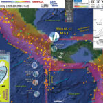
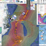
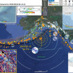
This region of Earth is one of the most seismically active in the past decade plus. This morning, as I was preparing for work, I got an email notifying me of an earthquake with a magnitude M = 7.5 located near New Ireland, Papua New Guinea.
https://earthquake.usgs.gov/earthquakes/eventpage/us70003kyy/executive
There are every type of plate boundary fault in this region. There are subduction zones, such as that forms the New Britain and San Cristobal trenches. There are transform faults, such as that responsible for the M 7.5 temblor. There are also spreading ridges, such as the one that forms the Manus Basin to the northwest of today’s quake.
I interpret this M 7.5 earthquake to be a left-lateral strike slip earthquake based on (1) the USGS mechanism (moment tensor), (2) our knowledge of the faulting in the region, and (3) historic analogue earthquake examples. There was an earthquake on a subparallel strike-slip fault on 8 March 2018 (here is the earthquake report for that event). Also in that report, I discuss an earthquake from November 2000 that had a magnitude M = 8.0.
After my work on the 28 September 2018 Donggala-Palu earthquake, landslides, and tsunami, I am open minded about the possibility of strike-slip earthquakes as having tsunamigenic potential. There are actually many examples of strike-slip earthquakes causing tsunami, including the 1999 Izmit, 2012 Wharton Basin, and the 2000 New Ireland earthquake too! (see Geist and Parsons, 2005 for more about the small 2000 tsunami.) There was initially a tsunami notification from tsunami.gov about the possibility of a tsunami. Here is a great website where I usually visit when I am looking for tsunami records on tide gage data. This is the closest gage to the quake, but it is not located optimally to record a small tsunami as might have been generated today (I checked).
The Weitin fault is a very active fault, with a slip rate of about 130 mm/yr (Tregoning et al, 1999, 2005). For a comparison, the San Andreas fault has a slip rate of about 25-35 mm/year. Here is a great treatise on the SAF.
There are also examples of earthquake triggering in this region. For example, the 2000.11.16 M 8.0 strike-slip earthquake triggered the 2000.11.16 M 7.8 thrust fault earthquake. It is not unreasonable to consider it possible that there may be triggered earthquakes from this M 7.5 earthquake. Of course, we won’t know until it happens because nobody has the capability to predict earthquakes (regardless of what the charlatans may claim).
The USGS has a variety of products associated with their earthquake pages. I use many of these products in these earthquake reports, so I especially appreciate them. One of the recently added products is a landslide and a liquefaction probability model output. Based on our knowledge of how earthquake release energy, and our knowledge of how earth materials respond to this energy release, people have developed models that allow us to estimate the possibility any given region may experience landslides or liquefaction. I spent some time discussing this in the 28 Sept. 2018 Donggala-Palu earthquake report here.

Below is my interpretive poster for this earthquake

I plot the seismicity from the past month, with color representing depth and diameter representing magnitude (see legend). I include earthquake epicenters from 1918-2018 with magnitudes M ≥ 3.0 in one version.
I plot the USGS fault plane solutions (moment tensors in blue and focal mechanisms in orange), possibly in addition to some relevant historic earthquakes.

  • I placed a moment tensor / focal mechanism legend on the poster. There is more material from the USGS web sites about moment tensors and focal mechanisms (the beach ball symbols). Both moment tensors and focal mechanisms are solutions to seismologic data that reveal two possible interpretations for fault orientation and sense of motion. One must use other information, like the regional tectonics, to interpret which of the two possibilities is more likely.
  • I also include the shaking intensity contours on the map. These use the Modified Mercalli Intensity Scale (MMI; see the legend on the map). This is based upon a computer model estimate of ground motions, different from the “Did You Feel It?” estimate of ground motions that is actually based on real observations. The MMI is a qualitative measure of shaking intensity. More on the MMI scale can be found here and here. This is based upon a computer model estimate of ground motions, different from the “Did You Feel It?” estimate of ground motions that is actually based on real observations.
  • I include the slab 2.0 contours plotted (Hayes, 2018), which are contours that represent the depth to the subduction zone fault. These are mostly based upon seismicity. The depths of the earthquakes have considerable error and do not all occur along the subduction zone faults, so these slab contours are simply the best estimate for the location of the fault.

    Magnetic Anomalies

  • In the map below, I include a transparent overlay of the magnetic anomaly data from EMAG2 (Meyer et al., 2017). As oceanic crust is formed, it inherits the magnetic field at the time. At different points through time, the magnetic polarity (north vs. south) flips, the North Pole becomes the South Pole. These changes in polarity can be seen when measuring the magnetic field above oceanic plates. This is one of the fundamental evidences for plate spreading at oceanic spreading ridges (like the Gorda rise).
  • Regions with magnetic fields aligned like today’s magnetic polarity are colored red in the EMAG2 data, while reversed polarity regions are colored blue. Regions of intermediate magnetic field are colored light purple.
  • We can see the roughly east-west trends of these red and blue stripes in the Woodlark Basin. These lines are parallel to the ocean spreading ridges from where they were formed. The stripes disappear at the subduction zone because the oceanic crust with these anomalies is diving deep beneath the upper plate, so the magnetic anomalies from the overlying plate mask the evidence for the lower plate.

    I include some inset figures. Some of the same figures are located in different places on the larger scale map below.

  • In the lower left corner is a figure from Oregon State University (Geology). This shows a cartoon view of the tectonic plates in the region. Note the subduction zone where the Solomon Sea late dives beneath the South Bismarck and Pacific plates. Of particular interest today is the transform (strike-slip) plate boundary between the North and South Bismarck plates.
  • In the upper left corner are two more detailed tectonic maps from Holm et al. (2019). The upper panel shows the plate boundary faults (active subduction zones are symbolized with dark triangles, fossil subd. zones are shown as open triangles). I plate a blue star int eh location of today’s earthquake (as for all inset figures). The lower panel shows the source of volcanic rocks as they have been derived from different subducted oceanic crust and overlying mantle. The geochemistry of these volcanic rocks helps us learn about the tectonic history of this complicated region.
  • The figure in the lower right corner (Holm et al., 2019) shows the current configuration of the different plate boundary faults. Note the left lateral strike-slip relative motion on the (labeled here) Bismarck Sea fault. When this fault crosses New Ireland, it splays into a series of different faults. The most active fault is the Weitin fault.
  • The figure in the upper right corner has lots of information, including cross sections showing the subduction zones (Holm et al., 2016). The oceanic crust created by spreading centers is highlighted for the Woodlark Basin, as well as the Manus Basin northwest of today’s M 7.5 earthquake. The cross section A-B shows these spreading centers.
  • Here is the map with a month’s seismicity plotted. This map includes magnetic anomaly data.

  • Here is the map with a century’s seismicity plotted for magnitudes M ≥ 7.5. Because of the complexity of this figure, the magnetic anomaly data are not included.

M 7.5 Landslide and Liquefaction Models

There are many different ways in which a landslide can be triggered. The first order relations behind slope failure (landslides) is that the “resisting” forces that are preventing slope failure (e.g. the strength of the bedrock or soil) are overcome by the “driving” forces that are pushing this land downwards (e.g. gravity). The ratio of resisting forces to driving forces is called the Factor of Safety (FOS). We can write this ratio like this:

FOS = Resisting Force / Driving Force

When FOS > 1, the slope is stable and when FOS < 1, the slope fails and we get a landslide. The illustration below shows these relations. Note how the slope angle α can take part in this ratio (the steeper the slope, the greater impact of the mass of the slope can contribute to driving forces). The real world is more complicated than the simplified illustration below.


Landslide ground shaking can change the Factor of Safety in several ways that might increase the driving force or decrease the resisting force. Keefer (1984) studied a global data set of earthquake triggered landslides and found that larger earthquakes trigger larger and more numerous landslides across a larger area than do smaller earthquakes. Earthquakes can cause landslides because the seismic waves can cause the driving force to increase (the earthquake motions can “push” the land downwards), leading to a landslide. In addition, ground shaking can change the strength of these earth materials (a form of resisting force) with a process called liquefaction.
Sediment or soil strength is based upon the ability for sediment particles to push against each other without moving. This is a combination of friction and the forces exerted between these particles. This is loosely what we call the “angle of internal friction.” Liquefaction is a process by which pore pressure increases cause water to push out against the sediment particles so that they are no longer touching.
An analogy that some may be familiar with relates to a visit to the beach. When one is walking on the wet sand near the shoreline, the sand may hold the weight of our body generally pretty well. However, if we stop and vibrate our feet back and forth, this causes pore pressure to increase and we sink into the sand as the sand liquefies. Or, at least our feet sink into the sand.
Below is a diagram showing how an increase in pore pressure can push against the sediment particles so that they are not touching any more. This allows the particles to move around and this is why our feet sink in the sand in the analogy above. This is also what changes the strength of earth materials such that a landslide can be triggered.


Below is a diagram based upon a publication designed to educate the public about landslides and the processes that trigger them (USGS, 2004). Additional background information about landslide types can be found in Highland et al. (2008). There was a variety of landslide types that can be observed surrounding the earthquake region. So, this illustration can help people when they observing the landscape response to the earthquake whether they are using aerial imagery, photos in newspaper or website articles, or videos on social media. Will you be able to locate a landslide scarp or the toe of a landslide? This figure shows a rotational landslide, one where the land rotates along a curvilinear failure surface.


Here is an excellent educational video from IRIS and a variety of organizations. The video helps us learn about how earthquake intensity gets smaller with distance from an earthquake. The concept of liquefaction is reviewed and we learn how different types of bedrock and underlying earth materials can affect the severity of ground shaking in a given location. The intensity map above is based on a model that relates intensity with distance to the earthquake, but does not incorporate changes in material properties as the video below mentions is an important factor that can increase intensity in places.

If we look at the map at the top of this report, we might imagine that because the areas close to the fault shake more strongly, there may be more landslides in those areas. This is probably true at first order, but the variation in material properties and water content also control where landslides might occur.
There are landslide slope stability and liquefaction susceptibility models based on empirical data from past earthquakes. The USGS has recently incorporated these types of analyses into their earthquake event pages. More about these USGS models can be found on this page.
I prepared some maps that compare the USGS landslide and liquefaction probability maps.

  • Here is the landslide probability map (Jessee et al., 2018). Below the poster I include the text from the USGS website that describes how this model is prepared. The topography and bathymetry come from the National Science Foundation funded GeoMapApp.


Nowicki Jessee and others (2018) is the preferred model for earthquake-triggered landslide hazard. Our primary landslide model is the empirical model of Nowicki Jessee and others (2018). The model was developed by relating 23 inventories of landslides triggered by past earthquakes with different combinations of predictor variables using logistic regression. The output resolution is ~250 m. The model inputs are described below. More details about the model can be found in the original publication. We modify the published model by excluding areas with slopes <5° and changing the coefficient for the lithology layer "unconsolidated sediments" from -3.22 to -1.36, the coefficient for "mixed sedimentary rocks" to better reflect that this unit is expected to be weak (more negative coefficient indicates stronger rock).To exclude areas of insignificantly small probabilities in the computation of aggregate statistics for this model, we use a probability threshold of 0.002.

  • Here is the liquefaction probability (susceptibility) map (Zhu et al., 2017). Note that the regions of low slopes in the valleys and coastal plains are the areas with a high chance of experiencing liquefaction.


Zhu and others (2017) is the preferred model for liquefaction hazard. The model was developed by relating 27 inventories of liquefaction triggered by past earthquakes to globally-available geospatial proxies (summarized below) using logistic regression. We have implemented the global version of the model and have added additional modifications proposed by Baise and Rashidian (2017), including a peak ground acceleration (PGA) threshold of 0.1 g and linear interpolation of the input layers. We also exclude areas with slopes >5°. We linearly interpolate the original input layers of ~1 km resolution to 500 m resolution. The model inputs are described below. More details about the model can be found in the original publication.

Other Report Pages

Some Relevant Discussion and Figures

    • Here is the generalized tectonic map of the region from Holm et al., 2015. I include the figure caption below as a blockquote.

    • Tectonic setting and mineral deposits of eastern Papua New Guinea and Solomon Islands. The modern arc setting related to formation of the mineral deposits comprises, from west to east, the West Bismarck arc, the New Britain arc, the Tabar-Lihir-Tanga-Feni Chain and the Solomon arc, associated with north-dipping subduction/underthrusting at the Ramu-Markham fault zone, New Britain trench and San Cristobal trench respectively. Arrows denote plate motion direction of the Australian and Pacific plates. Filled triangles denote active subduction. Outlined triangles denote slow or extinct subduction. NBP: North Bismarck plate; SBP: South Bismarck plate; AT: Adelbert Terrane; FT: Finisterre Terrane; RMF: Ramu-Markham fault zone; NBT: New Britain trench.

    • In earlier earthquake reports, I discussed seismicity from 2000-2015 here. The seismicity on the west of this region appears aligned with north-south shortening along the New Britain trench, while seismicity on the east of this region appears aligned with more east-west shortening. Here is a map that I put together where I show these two tectonic domains with the seismicity from this time period (today’s earthquakes are not plotted on this map, but one may see where they might plot).

    • Here is the slab interpretation for the New Britain region from Holm and Richards, 2013. I include the figure caption below as a blockquote.

    • 3-D model of the Solomon slab comprising the subducted Solomon Sea plate, and associated crust of the Woodlark Basin and Australian plate subducted at the New Britain and San Cristobal trenches. Depth is in kilometres; the top surface of the slab is contoured at 20 km intervals from the Earth’s surface (black) to termination of slabrelated seismicity at approximately 550 km depth (light brown). Red line indicates the locations of the Ramu-Markham Fault (RMF)–New Britain trench (NBT)–San Cristobal trench (SCT); other major structures are removed for clarity; NB, New Britain; NI, New Ireland; SI, Solomon Islands; SS, Solomon Sea; TLTF, Tabar–Lihir–Tanga–Feni arc. See text for details.

    • Here are the forward models for the slab in the New Britain region from Holm and Richards, 2013. I include the figure caption below as a blockquote.

    • Forward tectonic reconstruction of progressive arc collision and accretion of New Britain to the Papua New Guinea margin. (a) Schematic forward reconstruction of New Britain relative to Papua New Guinea assuming continued northward motion of the Australian plate and clockwise rotation of the South Bismarck plate. (b) Cross-sections illustrate a conceptual interpretation of collision between New Britain and Papua New Guinea.

    • Here is a map showing some detailed mapping of the Weitin fault (Lindley, 2006).

    • Weitin Fault, Southern New Ireland, showing trace of fault, topography and evidence used by Hohnen (1978) to tentatively suggest sinistral fault movement (after Hohnen, 1978).

    • This figure shows details of the regional tectonics (Holm et al., 2016). I include the figure caption below as a blockquote.

    • a) Present day tectonic features of the Papua New Guinea and Solomon Islands region as shown in plate reconstructions. Sea floor magnetic anomalies are shown for the Caroline plate (Gaina and Müller, 2007), Solomon Sea plate (Gaina and Müller, 2007) and Coral Sea (Weissel and Watts, 1979). Outline of the reconstructed Solomon Sea slab (SSP) and Vanuatu slab (VS)models are as indicated. b) Cross-sections related to the present day tectonic setting. Section locations are as indicated. Bismarck Sea fault (BSF); Feni Deep (FD); Louisiade Plateau
      (LP); Manus Basin (MB); New Britain trench (NBT); North Bismarck microplate (NBP); North Solomon trench (NST); Ontong Java Plateau (OJP); Ramu-Markham fault (RMF); San Cristobal trench (SCT); Solomon Sea plate (SSP); South Bismarck microplate (SBP); Trobriand trough (TT); projected Vanuatu slab (VS); West Bismarck fault (WBF); West Torres Plateau (WTP); Woodlark Basin (WB).

    • Here is a larger scale map showing lineaments (thin black lines) which represent structures formed at the spreading ridges (Lindley, 2006). These spreading ridges are perpendicular to the Weitin and sister transform faults (like the Sapom fault).

    • Map showing onshore structures of the Gazelle Peninsula and New Ireland and those interpreted from SeaMARC II sidescan backscatter data in the Eastern Bismarck Sea. BSSL, Bismarck Sea Seismic Lineation (BSSL). SeaMARC II backscatter data from which lineations have been picked are from Taylor et al. (1991 a-c). Modified after Madsen and Lindley (1994).

    • The interpretive poster above shows the 2007 M 8.1 tsunamigenic subduction zone earthquake. I presented information about this earthquake in a report from 22 Jan. 2017 here. Below are some of the interpretive posters from that report that show excellent examples of subduction zone earthquakes along the San Cristobal trench.
    • Here is my interpretive poster from the 12/17 M 7.9 Bougainville Earthquake, possibly (probably) related to today’s M 7.9 earthquake. This is my Earthquake Report for the 12/17 earthquake.

    Here is a visualization of the seismicity as presented by Dr. Steve Hicks.

    • Here are the maps from Holm et al. (2019) that show the sources of volcanic rocks in the region.

    • Tectonic setting of Papua New Guinea and Solomon Islands. A) Regional plate boundaries and tectonic elements. Light grey shading illustrates bathymetry <2000m below sea level indicative of continental or arc crust, and oceanic plateaus. The New Guinea Orogen comprises rocks of the New Guinea Mobile Belt and the Papuan Fold and Thrust Belt; Adelbert Terrane (AT); Aure-Moresby trough (AMT); Bougainville Island (B); Bismarck Sea fault (BSF); Bundi fault zone (BFZ); Choiseul Island (C); Feni Deep (FD); Finisterre Terrane (FT); Guadalcanal Island (G); Gazelle Peninsula (GP); Kia-Kaipito-Korigole fault zone (KKKF); Lagaip fault zone (LFZ); Malaita Island (M); Manus Island (MI); New Britain (NB); New Georgia Islands (NG); New Guinea Mobile Belt (NGMB); New Ireland (NI); Papuan Fold and Thrust Belt (PFTB); Ramu-Markham fault (RMF); Santa Isabel Island (SI); Sepik arc (SA); Weitin Fault (WF); West Bismarck fault (WBF); Willaumez-Manus Rise (WMR). Arrows indicate rate and direction of plate motion of the Australian and Pacific plates (MORVEL, DeMets et al., 2010); B) Pliocene-Quaternary volcanic centres and magmatic arcs related to this study. Figure modified from Holm et al. (2016). Subduction zone symbols with filled pattern denote active subduction; empty symbols denote extinct subduction zone or negligible convergence.

    • This is a series of plate reconstructions from Holm et al. (2019), the final panel is in the interpretive poster above.

    • Selected tectonic reconstructions and mineral deposit formation for key areas and times within the eastern Papua New Guinea and Solomon Islands region. A) Formation of the Panguna and Fauro Island Deposits above the interpreted subducted margin of the Solomon Sea plate-Woodlark Basin, and Mase deposit above the subducting Woodlark spreading center; B) Formation of the New Georgia deposits above the subducting Woodlark spreading center, and Guadalcanal deposits above the subducting margin of the Woodlark Basin; C) Formation of the Solwara deposits related to transtension along the Bismarck Sea fault above the subducting Solomon Sea plate, and deposits of the Tabar- Lihir-Tanga-Feni island arc chain related to upper plate extension (normal faulting indicated by hatched linework between New Ireland and Bougainville), while the Ladolam deposit forms above a tear in the subducting slab. Interpreted Solomon Sea slab (light blue shaded area for present-day) is from Holm and Richards (2013); the reconstructed surface extent or indicative trend of slab structure is indicated by the dashed red lines. Green regions denote the present-day landmass using modern coastlines; grey regions are indicative of crustal extent using the 2000m bathymetric contour. The reconstruction is presented here relative to the global moving hotspot reference frame, please see the reconstruction files in the supplementary material for specific reference frames.

Geologic Fundamentals

  • For more on the graphical representation of moment tensors and focal mechanisms, check this IRIS video out:
  • Here is a fantastic infographic from Frisch et al. (2011). This figure shows some examples of earthquakes in different plate tectonic settings, and what their fault plane solutions are. There is a cross section showing these focal mechanisms for a thrust or reverse earthquake. The upper right corner includes my favorite figure of all time. This shows the first motion (up or down) for each of the four quadrants. This figure also shows how the amplitude of the seismic waves are greatest (generally) in the middle of the quadrant and decrease to zero at the nodal planes (the boundary of each quadrant).

  • Here is another way to look at these beach balls.
  • There are three types of earthquakes, strike-slip, compressional (reverse or thrust, depending upon the dip of the fault), and extensional (normal). Here is are some animations of these three types of earthquake faults. The following three animations are from IRIS.
  • Strike Slip:

    Compressional:

    Extensional:

  • This is an image from the USGS that shows how, when an oceanic plate moves over a hotspot, the volcanoes formed over the hotspot form a series of volcanoes that increase in age in the direction of plate motion. The presumption is that the hotspot is stable and stays in one location. Torsvik et al. (2017) use various methods to evaluate why this is a false presumption for the Hawaii Hotspot.

  • A cutaway view along the Hawaiian island chain showing the inferred mantle plume that has fed the Hawaiian hot spot on the overriding Pacific Plate. The geologic ages of the oldest volcano on each island (Ma = millions of years ago) are progressively older to the northwest, consistent with the hot spot model for the origin of the Hawaiian Ridge-Emperor Seamount Chain. (Modified from image of Joel E. Robinson, USGS, in “This Dynamic Planet” map of Simkin and others, 2006.)

  • Here is a map from Torsvik et al. (2017) that shows the age of volcanic rocks at different locations along the Hawaii-Emperor Seamount Chain.

  • Hawaiian-Emperor Chain. White dots are the locations of radiometrically dated seamounts, atolls and islands, based on compilations of Doubrovine et al. and O’Connor et al. Features encircled with larger white circles are discussed in the text and Fig. 2. Marine gravity anomaly map is from Sandwell and Smith.

  • Here is a great tweet that discusses the different parts of a seismogram and how the internal structures of the Earth help control seismic waves as they propagate in the Earth.

    Social Media

    References:

  • Baldwin, S.L., Monteleone, B.D., Webb, L.E., Fitzgerald, P.G., Grove, M., and Hill, E.J., 2004. Pliocene eclogite exhumation at plate tectonic rates in eastern Papua New Guinea in Nature, v. 431, p/ 263-267, doi:10.1038/nature02846.
  • Baldwin, S.L., Fitzgerald, P.G., and Webb, L.E., 2012. Tectonics of the New Guinea Region, Annu. Rev. Earth Planet. Sci., v. 40, pp. 495-520.
  • Cloos, M., Sapiie, B., Quarles van Ufford, A., Weiland, R.J., Warren, P.Q., and McMahon, T.P., 2005, Collisional delamination in New Guinea: The geotectonics of subducting slab breakoff: Geological Society of America Special Paper 400, 51 p., doi: 10.1130/2005.2400.
  • Hamilton, W.B., 1979. Tectonics of the Indonesian Region, USGS Professional Paper 1078.
  • Frisch, W., Meschede, M., Blakey, R., 2011. Plate Tectonics, Springer-Verlag, London, 213 pp.
  • Geist, E. L., and T. Parsons (2005), Triggering of tsunamigenic aftershocks from large strike-slip earthquakes: Analysis of the November 2000 New Ireland earthquake sequence, Geochem. Geophys. Geosyst., 6, Q10005, https://doi.org/10.1029/2005GC000935.
  • Hayes, G., 2018, Slab2 – A Comprehensive Subduction Zone Geometry Model: U.S. Geological Survey data release, https://doi.org/10.5066/F7PV6JNV.
  • Highland, L.M., and Bobrowsky, P., 2008. The landslide handbook—A guide to understanding landslides, Reston, Virginia, U.S. Geological Survey Circular 1325, 129 p.
  • Holm, R. and Richards, S.W., 2013. A re-evaluation of arc-continent collision and along-arc variation in the Bismarck Sea region, Papua New Guinea in Australian Journal of Earth Sciences, v. 60, p. 605-619.
  • Holm, R.J., Richards, S.W., Rosenbaum, G., and Spandler, C., 2015. Disparate Tectonic Settings for Mineralisation in an Active Arc, Eastern Papua New Guinea and the Solomon Islands in proceedings from PACRIM 2015 Congress, Hong Kong ,18-21 March, 2015, pp. 7.
  • Holm, R.J., Rosenbaum, G., Richards, S.W., 2016. Post 8 Ma reconstruction of Papua New Guinea and Solomon Islands: Microplate tectonics in a convergent plate boundary setting in Eartth Science Reviews, v. 156, p. 66-81.
  • Holm, R.J., Tapster, S., Jelsma, H.A., Rosenbaum, G., and Mark, D.F., 2019. Tectonic evolution and copper-gold metallogenesis of the Papua New Guinea and Solomon Islands region in Ore Geology Reviews, v. 104, p. 208-226, https://doi.org/10.1016/j.oregeorev.2018.11.007
  • Jessee, M.A.N., Hamburger, M. W., Allstadt, K., Wald, D. J., Robeson, S. M., Tanyas, H., et al. (2018). A global empirical model for near-real-time assessment of seismically induced landslides. Journal of Geophysical Research: Earth Surface, 123, 1835–1859. https://doi.org/10.1029/2017JF004494
  • Johnson, R.W., 1976, Late Cainozoic volcanism and plate tectonics at the southern margin of the Bismarck Sea, Papua New Guinea, in Johnson, R.W., ed., 1976, Volcanism in Australia: Amsterdam, Elsevier, p. 101-116
  • Keefer, D.K., 1984. Landslides Caused by Earthquakes in GSA Bulletin, v. 95, p. 406-421
  • Kreemer, C., G. Blewitt, E.C. Klein, 2014. A geodetic plate motion and Global Strain Rate Model in Geochemistry, Geophysics, Geosystems, v. 15, p. 3849-3889, https://doi.org/10.1002/2014GC005407.
  • Lindley, I.D., 2006. Extensional and vertical tectonics in the New Guinea islands: implications for island arc evolution in Annals of Geophysics, suppl to v. 49, no. 1, p. 403-426
  • Meyer, B., Saltus, R., Chulliat, a., 2017. EMAG2: Earth Magnetic Anomaly Grid (2-arc-minute resolution) Version 3. National Centers for Environmental Information, NOAA. Model. https://doi.org/10.7289/V5H70CVX
  • Müller, R.D., Sdrolias, M., Gaina, C. and Roest, W.R., 2008, Age spreading rates and spreading asymmetry of the world’s ocean crust in Geochemistry, Geophysics, Geosystems, 9, Q04006, https://doi.org/10.1029/2007GC001743
  • Tregoning, P., Jackong, R.J., McQueen, H., Lambeck, K., Stevens, C., Little, R.P., Curley, R., and Rosa, R., 1999. Motion of the South Bismarck Plate, Papua New Guinea in GRL, v. 26, no. 23, p. 3517-3520
  • Tregoning, P., McQueen, H., Lambeck, K., Jackson, R. Little, T., Saunders, S., and Rosa, R., 2000. Present-day crustal motion in Papua New Guinea, Earth Planets and Space, v. 52, pp. 727-730.
  • Tregoning, P., Sambridge, M., McQueen, H., Toulin, S., and Nicholson, T., 2005. Motion of the South Bismarck Plate, Papua New Guinea in GJI, v. 160, p. 1103-111, https://doi.org/10.111/j.1365-246X.2005.02567.x
  • USGS, 2004. Landslide Types and Processes, U.S. Geological Survey Fact Sheet 2004-3072
  • Zhu, J., Baise, L. G., Thompson, E. M., 2017, An Updated Geospatial Liquefaction Model for Global Application, Bulletin of the Seismological Society of America, 107, p 1365-1385, doi: 0.1785/0120160198

Return to the Earthquake Reports page.


Earthquake Report: Panamá

There was just now an earthquake beneath Panamá. The major plate boundary in the region is a subduction zone (convergent plate boundary) where the Cocos and Nazca plates dive northwards beneath the Caribbean plate forming the Middle America trench (MAT).
This magnitude M = 6.1 earthquake appears to be associated with the transform plate boundary (strike-slip fault) that is formed between the Cocos and Nazca plates. I initially interpreted the earthquake mechanism (e.g. moment tensor) shows this to be a strike-slip earthquake along the Panamá fracture zone (PFZ). However, the earthquake is not currently deep enough according to the USGS Slab 2.0 data (that shows the depth of the megathrust subduction zone, or the top of the downgoing oceanic crust/slab). This is still possible, but it is also possible that this is in the upper plate, the Caribbean plate.
If this is in the upper plate (seems more probable), then there are several reasons for the temblor. Perhaps the PFZ is causing differential stress in the overriding plate (causing strike-slip faults to form subparallel to the PFZ and sister faults). Perhaps there is oblique relative plate motion, that is causing strain and slip partitioning in upper plate crustal faults. Perhaps there is some other complicated faulting in the upper plate that exists for some other reason (e.g. pre-existing structures inherited from the tectonic history). OR, it may be due to a combination of any of these possibilities. The fact that this earthquake (and a Christmas temblor in 2003) are aligned with the PFZ suggests that these quakes may be related to the PFZ. As Mr. Spock (Star Trek) would say, “fascinating.”
I have some early reports for quakes along this fz, though the quality of my reports have improved over time. See the May 2014 and January 2015 reports.
The Panama fracture zone (PFZ) has a few sister fracture zones, subparallel dextral (right-lateral) strike-slip faults that have been studied by looking at seismicity and structures of the seafloor. There was a series of large earthquakes in the region south of the MAT in 1934 (Camacho, 1991) ewith the largest magnitude quake at M = 7.5. Earthquakes in the magnitude 6 range are quite common for this system, with temblors M ≥ 6 over once a year.
After tweeting this report, Dr. Kristen Morell (assistant professor at U.C. Santa Barbara) pointed out to me that they did lots of work on the tectonics in the region for their Ph.D. research. I have added some figures from her work below. Morell shows that there are upper plate crustal faults that are associated with the PFZ. Dr. Morell uses a variety of methods to come to this conclusion, including geomorphology (always a great tool), fault mapping (and cross sections of thrust faults and folds), relative plate motions and reconstructions, exhumation analysis, etc. These articles are fundamental to our understanding in this region and we are lucky to have them.

Below is my interpretive poster for this earthquake

I plot the seismicity from the past month, with color representing depth and diameter representing magnitude (see legend). I include earthquake epicenters from 1918-2018 with magnitudes M ≥ 3.0 in one version.
I plot the USGS fault plane solutions (moment tensors in blue and focal mechanisms in orange), possibly in addition to some relevant historic earthquakes.

  • I placed a moment tensor / focal mechanism legend on the poster. There is more material from the USGS web sites about moment tensors and focal mechanisms (the beach ball symbols). Both moment tensors and focal mechanisms are solutions to seismologic data that reveal two possible interpretations for fault orientation and sense of motion. One must use other information, like the regional tectonics, to interpret which of the two possibilities is more likely.
  • I also include the shaking intensity contours on the map. These use the Modified Mercalli Intensity Scale (MMI; see the legend on the map). This is based upon a computer model estimate of ground motions, different from the “Did You Feel It?” estimate of ground motions that is actually based on real observations. The MMI is a qualitative measure of shaking intensity. More on the MMI scale can be found here and here. This is based upon a computer model estimate of ground motions, different from the “Did You Feel It?” estimate of ground motions that is actually based on real observations.
  • I include the slab 2.0 contours plotted (Hayes, 2018), which are contours that represent the depth to the subduction zone fault. These are mostly based upon seismicity. The depths of the earthquakes have considerable error and do not all occur along the subduction zone faults, so these slab contours are simply the best estimate for the location of the fault. Note how the slab contours end at the longitude of the PFZ.

    Magnetic Anomalies

  • In the map below, I include a transparent overlay of the magnetic anomaly data from EMAG2 (Meyer et al., 2017). As oceanic crust is formed, it inherits the magnetic field at the time. At different points through time, the magnetic polarity (north vs. south) flips, the North Pole becomes the South Pole. These changes in polarity can be seen when measuring the magnetic field above oceanic plates. This is one of the fundamental evidences for plate spreading at oceanic spreading ridges (like the Gorda rise).
  • Regions with magnetic fields aligned like today’s magnetic polarity are colored red in the EMAG2 data, while reversed polarity regions are colored blue. Regions of intermediate magnetic field are colored light purple.
  • We can see the roughly east-west trends of these red and blue stripes. These lines are parallel to the ocean spreading ridges from where they were formed, at the Galapagos Spreading Ridge.

    I include some inset figures. Some of the same figures are located in different places on the larger scale map below.

  • In the upper right corner is a map from Hoernle et al. (2002) that shows the general plate tectonic configuration in this region. We can see the subduction zones, the spreading ridge, and the transform faults (e.g. the PFZ).
  • In the lower left corner there is a figure that shows how the spreading ridges (extensional plate boundaries) have been offset by the fracture zones (transform plate boundaries). Note how some of the spreading ridges are inactive (Meschede and Barckhausen, 2000)
  • In the upper left corner is a large scale map showing the detailes of the magnetic anomalies as they relate to the faults in the region ((Marcaillou et al., 2006).
  • In the lower right corner is a map that shows the details of the different earthquakes during the 1934 sequence (Camacho, 1991).
  • Here is the map with a month’s seismicity plotted.

  • Here is the map with a century’s seismicity plotted.

  • Here is the map with the Global Earthquake Model (GEM) strain map as an overlay (Kreemer et al., 2014). Strain is a quantification of the amount of deformation of the Earth over time. Technically, it is the change in shape (length, volume) per unit time. Note how the strain is localized along the subduction zone, as well as along the PFZ.

Other Report Pages

Some Relevant Discussion and Figures

  • Here is the tectonic overview figure from Hoernle et al. (2002).

  • Gala´pagos Islands and hotspot tracks (Cocos, Coiba, Malpelo, and Carnegie Ridges), igneous complexes in Central America with Gala´pagos geochemical affinities, and western portion of Caribbean plate. Is. is Island, S.C. is spreading
    center.

  • This is another good overview map that shows the spreading center that creates the Nazca and Cocos plates (Coates et al., 2004).

  • Map of southern Central America (dark shading) and the Panama microplate (pale shading). Darien is picked out in pale shading. Dashed lines with teeth mark zones of convergence; zippered line is Panama-Colombia suture. Very heavy dashed line marks location of Neogene volcanic arc; black circles mark Paleogene-Eocene volcanic arc. NPDB – North Panama deformed belt; SPDB – South Panama deformed belt; PFZ – Panama fracture zone. Principal Neogene sedimentary basins located by striped ovals.

  • Here is a map showing an early interpretation of the magnetic anomalies of the Panama Basin (Lonsdale and Klitgord, 1978). The following 2 figures show an example of how shipboard measurements of magnetic intensity are interpreted for the seafloor shown in this figure. The gray bands are parts of the oceanic crust that share a similar magnetic polarity and a similar range in ages. They also present their interpretations of the crustal structures in the region. Recall that this map was prepared long before we had the excellent detailed bathymetry data that we may view in Google Earth (prepared as an inversion of gravity data collected from satellites and the Space Shuttle). Many of the subsequent interpretations of the tectonics in the region is based on this initial analysis.

  • Crustal structure between Malpelo and Panama, showing 1965 to 1975 epicenters (defining present plate boundaries), magnetic anomalies, tracks of profiles shown in Figures 6 and 8, and locations of sampling sites.

  • Here is a map showing the magnetic intensity observations as recorded from research cruises (Lonsdale and Klitgord, 1978). The wiggles are shown along the ship tracklines. The next figure shows one example of these magnetic profiles and how they interpret these data into the magnetic anomaly map of the seafloor.

  • Magnetic anomalies between Malpelo and Carnegie Ridges, numbered according to time scales listed in caption of Figure 2. Note anomaly 5 to 5B sequence along long 81°W, mirrored around extinct Malpelo rift spreading center at lat 1°40’N. Magnetic anomalies on western (Costa Rica rift) segment are from Hey and others (1977). Tracks are labeled for Conrad 11.11 (CON 11) Yaloc 69 (Y 69), Iguana 3, Cocotow 2 (CCTW 2), Cocotow 3 (CCTW 3), F. Drake 3 (FD 3), and some lines of Oceanographer 70 (OC 70). Unlabeled profiles on Costa Rica rift are from Oceanographer 69; those on Malpelo rift are from Oceanographer 70.

  • Here is the profile from Malpelo Ridge to Carnegie Ridge (Lonsdale and Klitgord, 1978). They present the observations compared to their modeled results at the top and a bathymetric profile along with sediment thickness on the bottom.

  • Profile of Cocotow 3 traverse between Malpelo and Carnegie Ridges (see Fig. 4 for location). Synthetic magnetic profile was generated using reversal time scale discussed in Figure 2 caption, spreading rates indicated at top of this figure, magnetization of 4 A/m, and magnetized layer that is 500 m thick and has an upper surface that coincides with basement relief. Note that anomaly match is poor
    within 50 to 100 km of Carnegie and Malpelo Ridges. Fit could have been improved by postulating a somewhat faster spreading rate for this region, but even so, we could not achieve as good a match as for central part of profile.

  • This is the result of their analyses (Lonsdale and Klitgord, 1978). These authors prepared a tectonic reconstruction given their knowledge of crustal structures and magnetic anomaly data.

  • Tectonic reconstructions tracing inferred history of eastern Panama Basin. (A) Middle Oligocene: Farallon plate interacting with Caribbean and South American plates, just before splitting into Nazca and Cocos plates. (B) Middle Miocene: Malpelo and Carnegie Ridges are being formed by hot spot centered on Nazca plate near axis of Nazca-Cocos spreading and are being continuously separated by spreading at boundary. (C) Late Miocene: slowdown of spreading on Malpelo rift, rejuvenation of fracture zone at long 83°W, and cessation of subduction at Panama Trench. (D) Early Pliocene: continued northward migration of Cocos Ridge, stagnation of Malpelo Ridge, and uplift of Coiba Ridge near Nazca-Cocos-Caribbean triple junction. (E) Pleistocene: Cocos and Carnegie Ridges have just arrived at Middle America and Ecuador Trenches, and triple junction has jumped west from Coiba to Panama fracture zone.

  • Here is the map from Meschede and Barchkausem (2000) that shows the complexity of the spreading ridges and the fracture zones in the region.

  • Overview of the eastern Panama Basin (modified from Meschede et al., 1998). Numbers indicate the ages of oceanic crust. The distribution of extinct spreading systems is from Meschede et al. (1998). CNS = Cocos-Nazca spreading system. RSB = rough/smooth boundary.

  • Here is the figure from Camacho (1991) showing their analysis of the faults and earthquake mechanisms from teh 1934 series of earthquakes (and others too). I include their focal mechanism in the posters above.

  • Map depicting lhe southwestern Panama continental manin and lhe Panama-Coiba Fracture Zone wilh some of its characteristic focal mechanisms.

  • Here is the detailed map from Marcaillou et al. (2006) showing the ages of the seafloor for the Panama Basin (the oceanic crust near and east of the PFZ).

  • Interpretation of the pattern of crustal isochrons (Hardy 1991; Lonsdale 2005) and plate boundaries in the Panama Basin (modified from Lonsdale 2005). Earthquakes (black dots) and fault plane solution are from the Harvard University archive of centroid-moment tensor solutions. Plain lines are active spreading axis and transform faults: Costa Rica Rift (CRR) and Panama Fracture Zone (PFZ). Dashed and dotted lines are fossil spreading axis and transform faults: Buenaventura Rift (BR), Malpelo Rift (MR), Coiba Fracture Zone (CFZ) and Yaquina Graben. Possible spreading activity along Sandra Rift (SR) is still in discussion.

  • UPDATE: Here are some key figures from Dr. Morell’s research.
  • The interaction of the Cocos Ridge with the MAT appears to be a key part of the tectonics associated with the PFZ. Here is the plate tectonic map from Morell et al. (2012).
  • My original maps included left-lateral strike-slip arrows on the subduction zone east of the PFZ because I had interpreted this as likely given the obliquity of relative plate motion there, but I was unsure if this was reasonable (I had not seen any maps showing this). Given the analysis by Dr. Morell, I have replaced these arrows in the interpretive posters. Sometimes it is good to go with one’s interpretations of their observations, regardless if they find these interpretations elsewhere. Good lesson.

  • (a) Digital elevation model of the plate tectonic setting surrounding the Cordillera de Talamanca (CT), southern Costa Rica and Cordillera Central (CC), western Panama. Tectonic plates shown are the Cocos plate (CO), Nazca plate (NZ), Caribbean plate (CA), Panama microplate (PM), with plate velocities relative to a fixed CA plate [Bird, 2003; DeMets et al., 1990; DeMets, 2001; Jin and Zhu, 2004; Kellogg and Vega, 1995]. MAT, Middle America Trench; EPR, East Pacific Rise; CNS-2, Cocos-Nazca-Spreading; PTJ, Panama Triple Junction; PFZ, Panama Fracture Zone; BFZ, Balboa Fracture Zone; CFZ, Coiba Fracture Zone; NP, Nicoya Peninsula; AG, Aguacate Range; OP, Osa Peninsula; BP, Burica Peninsula; FCTB, Fila Costeña Thrust Belt; NPDB, North Panama Deformed Belt; TV, Tisingal Volcano; IV, Irazú volcano; BV, Barú volcano; YV, La Yeguada volcano; EV, El Valle volcano. Bathymetric data supplied by ETOPO1 combined from Amante and Eakins [2009], Smith and Sandwell [1997], and Ranero et al. [2003]. Topography supplied by CGIR-CSI based on NASA’s SRTM4 data set. White triangles indicate active volcanoes. Yellow dashed lines indicate on-land projection of Cocos Ridge boundaries. (b) Inset showing location of Figure 1a based on ETOPO1 data. SA refers to the South American plate. (c) Velocity triangle for Panama Triple Junction. CR represents the axis of the Cocos Ridge. Red lines denote the PM-CO and PM-NZ vectors, respectively. Numbers shown are in mm/yr.

  • This figure shows how Dr. Morell interprets how the PFZ projects beneath the upper plate (Morell et al. (2013). Note how the faults in the Fila Costeña Thrust Belt terminate where this tear is projected.

  • Map of southern Central America, showing plate tectonic setting surrounding the Panama triple junction (PTJ) and Barú Volcano based on a stable Caribbean plate (DeMets et al., 1990; Kellogg and Vega, 1995; DeMets, 2001; Bird, 2003). MAT—Middle America Trench; CO—Cocos plate; NZ—Nazca plate; CA— Caribbean plate; PM—Panama micro plate; PTJ—Panama triple junction; PFZ—Panama fracture zone; BFZ—Balboa fracture zone; CFZ—Coiba fracture zone; TV—Tisingal Volcano; OP—Osa Peninsula; BP—Burica Peninsula; VG— Valle General. Elevations are based on National Aeronautics and Space Administration’s (NASA) SRTM v4 imagery. Bathymetry is combined from ETOPO1 and Ranero et al. (2003). Thrusts and shortening estimates outlined for Fila Costeña thrust belt are combined from Sitchler et al. (2007), Fisher et al. (2004), and Morell et al. (2008). Fault traces on Burica Peninsula are from Morell et al. (2011a) and back arc is from Brandes et al. (2007). Contour interval for bathymetry is 250 m.

  • Here is a map that shows how geomorphology can be used to interpret the tectonics of a region (Morell et al., 2013). The color of the stream channel networks represents the steepness of those channels. We can interpret steeper channels to represent regions of higher (or more recent) tectonic uplift rates.
  • Note how the steeper channels are to the west of the projection of the PFZ tear, coincident with the eastern termination of the Fila Costeña Thrust Belt.

  • Map of normalized steepness (ksn) values calculated over a 0.5 km window for drainage basins >107 m2 and excluding valley bottoms for Cordillera de Talamanca and western Cordillera Central. Numbers in northeastern flank of Talamanca correspond to knickpoint numbers shown in Table 2. The locations of longitudinal profiles in Figure 7 are marked as A, B and C, respectively. Faults shown in the Fila Costeña are based on Fisher et al. [2004], Morell et al. [2008], and Sitchler et al. [2007]. Faults drawn in the Limón back arc are approximated from topographic lineaments. Location shown in Figure 1. Base map sourced from DEM draped over slope map derived from SRTM data set. Inset in upper right is simplified geologic map for Cordillera de Talamanca region based on Denyer and Alvarado [2007].

  • Here is a larger scale map showing the geological mapping or late Cretaceous, Tertiary, and Quaternary rock units, and the detailed fault mapping (Morell et al., 2009). The inset shows a shaded relief map showing some of the north-south faults in the upper plate, which are suggested to reflect the crustal response of the PFZ in the upper plate.

  • Simplified geologic map of the southeast Fila Costeña Thrust Belt in the inner forearc of Costa Rica and western Panama (see Fig. 1 for location). Combined data from Sitchler et al. (in press) and this study, revised after Kolarsky and Mann (1995) and Mora (1979). Although the thrust belt continues to the northwest, we focus on the southeast termination. Black boxes indicate location of Figs. 3 and 5. OPFZ = On-land projection of the Panama Fracture Zone. Geology is draped on 90-m DEM supplied by NASA’s SRTM-3 dataset. Stratigraphic column modified after Sitchler et al. (in press), Phillips (1983) and Fisher et al. (2004). Inset A shows shaded DEM of area in white dotted box denoting scarps visible for right-lateral faults A and B based on SRTM-3 dataset.

  • This is an even more large scale map showing strike and dip measurement of the thrust faults mapped in the above figure, as well as more details of the north-south strike-slip raults. Note how they offset some of the thrust faults with a right-lateral _dextral_sense of motion. This is the same sense of motion as the PFZ. This is probably not a coincidence!

  • Bedrock geologic map of the southeastern termination of the Fila Costeña Thrust Belt showing strike and dip measurements within thrust sheets that dip to the northeast. The southeastern termination of the thrust belt roughly coincides with the on-land projection of the Panama Fracture Zone (OPFZ, red dashed line), which is migrating to the southeast with the Panama Triple Junction. F1, F2, F3, F4, and F5 refer to thrust faults 1, 2, 3, 4 and 5, respectively. Cross-sections show locations of balanced cross-sections in Fig. 4. All fault traces and contacts are approximated. Inset index map shows figure location in red box relative to the on-land projection of the Panama Fracture Zone.

  • The following two figures show the Tertiary to recent tectonic reconstructions from Morell (2015). These reconstructions are based on relative plate motion rates as constrained by magnetic anomalies mapped in the oceanic crust, as well as GPS and plate circuit relative plate motions from other researchers (e.g. MOREVEL from DeMets et al., 2010 and others). Frist we see the Morell (2015) magnetic anomaly map, then the plate history maps.

  • Digital elevation model [Smith and Sandwell, 1997; Amante and Eakins, 2009] showing Panama Basin and seafloor magnetic anomaly data surrounding the southern Central America subduction zone [Lonsdale and Klitgord, 1978; Wilson and Hey, 1995; Barckhausen et al., 2001; Lonsdale, 2005] based on chron time scale of Cande and Kent [1995]. The 22000 m contour is shown for prominent bathymetric features in the region, including Malpelo Ridge (MaR) and Coiba Ridge (CoR). BFZ, Balboa Fracture Zone; CFZ, Coiba Fracture Zone; CNS, Cocos-Nazca spreading center; COL, Colombia; CR, Costa Rica; EC, Ecuador; GHS, Galapagos hot spot; MR, Malpelo Rift; MAT, Middle America Trench; MoR, Morgan Rift; NI, Nicaragua; PA, Panama; PFZ, Panama Fracture Zone; SR, Sandra Rift; YG, Yaquina Graben. Inset: Present day plate boundaries of Cocos (CO), Nazca (NZ), Caribbean (CA), and South American (SA) plates. East Pacific Rise (EPR) and Cocos-Nazca Spreading Center (CNS) are also shown.


    Plate reconstruction models for the Cocos (CO) and Nazca (NZ) plates relative to the Caribbean plate from 4 Ma to recent. BFZ, Balboa Fracture Zone; CaR, Carnegie Ridge; CFZ, Coiba Fracture Zone; CNS, crust derived from the Cocos-Nazca spreading center; CocR, Cocos Ridge; CoR, Coiba Ridge; CR, Costa Rica; EPR, crust derived from the East Pacific Rise; GH, Galapagos hot spot; MaR, Malpelo Ridge; MoR, Morgan Rift; MR, Malpelo Rift; PA, Panama; PFZ, Panama Fracture Zone; PTJ, Panama Triple Junction; RSB, rough-smooth boundary; SMD, seamount domain; SR, Sandra Ridge; YG, Yaquina Graben.


    Plate reconstruction models for the Cocos and Nazca plates relative to the Caribbean plate from 6 to 10 Ma. CaR, Carnegie Ridge; CFZ, Coiba Fracture Zone; CNS, crust derived from the Cocos-Nazca spreading center; CocR, Cocos Ridge; CR, Costa Rica; EPR, crust derived from the East Pacific Rise; GH, Galapagos hot spot; MaR, Malpelo Ridge; MR, Malpelo Rift; PA, Panama; PFZ, Panama Fracture Zone; PTJ, Panama Triple Junction; SMD, seamount domain, SR, Sandra Ridge; YG, Yaquina Graben.

Geologic Fundamentals

  • For more on the graphical representation of moment tensors and focal mechanisms, check this IRIS video out:
  • Here is a fantastic infographic from Frisch et al. (2011). This figure shows some examples of earthquakes in different plate tectonic settings, and what their fault plane solutions are. There is a cross section showing these focal mechanisms for a thrust or reverse earthquake. The upper right corner includes my favorite figure of all time. This shows the first motion (up or down) for each of the four quadrants. This figure also shows how the amplitude of the seismic waves are greatest (generally) in the middle of the quadrant and decrease to zero at the nodal planes (the boundary of each quadrant).

  • Here is another way to look at these beach balls.
  • There are three types of earthquakes, strike-slip, compressional (reverse or thrust, depending upon the dip of the fault), and extensional (normal). Here is are some animations of these three types of earthquake faults. The following three animations are from IRIS.
  • Strike Slip:

    Compressional:

    Extensional:

  • This is an image from the USGS that shows how, when an oceanic plate moves over a hotspot, the volcanoes formed over the hotspot form a series of volcanoes that increase in age in the direction of plate motion. The presumption is that the hotspot is stable and stays in one location. Torsvik et al. (2017) use various methods to evaluate why this is a false presumption for the Hawaii Hotspot.

  • A cutaway view along the Hawaiian island chain showing the inferred mantle plume that has fed the Hawaiian hot spot on the overriding Pacific Plate. The geologic ages of the oldest volcano on each island (Ma = millions of years ago) are progressively older to the northwest, consistent with the hot spot model for the origin of the Hawaiian Ridge-Emperor Seamount Chain. (Modified from image of Joel E. Robinson, USGS, in “This Dynamic Planet” map of Simkin and others, 2006.)

  • Here is a map from Torsvik et al. (2017) that shows the age of volcanic rocks at different locations along the Hawaii-Emperor Seamount Chain.

  • Hawaiian-Emperor Chain. White dots are the locations of radiometrically dated seamounts, atolls and islands, based on compilations of Doubrovine et al. and O’Connor et al. Features encircled with larger white circles are discussed in the text and Fig. 2. Marine gravity anomaly map is from Sandwell and Smith.

  • Here is a great tweet that discusses the different parts of a seismogram and how the internal structures of the Earth help control seismic waves as they propagate in the Earth.

    References:

  • Camacho, E., 1991. The Puerto Armuelles Earthquake (southwestern Panama) of July 18, 1934 in Rev. Geol. Amer. Central, v. 13, p. 1-13.
  • Coates, A.G., Collins, L.S., Aubry, M.-P., and Berggren, W.A., 2004. The Geology of the Darien, Panama, and the late Miocene-Pliocene collision of the Panama arc with northwestern South America in GSA Bulletin, v. 116, no. 11/12, p. 1327-1344, doi: 10.1130/B25275.1;
  • Frisch, W., Meschede, M., Blakey, R., 2011. Plate Tectonics, Springer-Verlag, London, 213 pp.
  • Hayes, G., 2018, Slab2 – A Comprehensive Subduction Zone Geometry Model: U.S. Geological Survey data release, https://doi.org/10.5066/F7PV6JNV.
  • Hoernle, K., van den Bogaard, P., Werner,R., Lissinna, B., Hauff, F., Alvarado, G., Garbe-Schönberg, D., 2002. Missing history (16–71 Ma) of the Gala´pagos hotspot: Implications
    for the tectonic and biological evolution of the Americas in Geology, v. 30, no. 9, p. 795-798
  • Kreemer, C., G. Blewitt, E.C. Klein, 2014. A geodetic plate motion and Global Strain Rate Model in Geochemistry, Geophysics, Geosystems, v. 15, p. 3849-3889, https://doi.org/10.1002/2014GC005407.
  • Lonsdale, P. and Klitgord, K.D., 1978. Structure and tectonic history of the eastern Panama Basin in GSA Bulletin, v. 89, p. 981-999
  • Morell, K. D., Fisher, D.M., Gardner, T.W., 2008. Inner forearc response to subduction of the Panama Fracture Zone, southern Central America in EPSL, v. 268, p. 82-85, http://doi.org/10.1016/j.epsl.2007.09.039
  • Morell, K. D., Kirby, E., Fisher, D. M., and van Soest, M. 2012. Geomorphic and exhumational response of the Central American Volcanic Arc to Cocos Ridge subduction in J. Geophys. Res., v. 117, B04409, https://doi.org/10.1029/2011JB008969.
  • Morell, K. D., Gardner, T.W., Fisher, D.M., Idleman, B.D., and Zellner, H.M., 2013. Active thrusting, landscape evolution, and late Pleistocene sector collapse of Barú Volcano above the Cocos-Nazca slab tear, southern Central America in GSA Bulletin, v. 125, no. 7/8, p. 1301-1318 https://doi.org/10.1130/B30771.1
  • Morell, K. D., 2015. Late Miocene to recent plate tectonic history of the southern Central America convergent margin in Geochem. Geophys. Geosyst., v. 16, p. 3362–3382, https://doi.org/10.1002/2015GC005971.
  • Meyer, B., Saltus, R., Chulliat, a., 2017. EMAG2: Earth Magnetic Anomaly Grid (2-arc-minute resolution) Version 3. National Centers for Environmental Information, NOAA. Model. https://doi.org/10.7289/V5H70CVX
  • Marcaillou, B., Charvis, P., and Collot, J.-V., 2006. Structure of the Malpelo Ridge (Colombia) from seismic and gravity modelling in Mar Geophys Res., DOI 10.1007/s11001-006-9009-y
  • Meschede, M., and Barckhausen, U., 2000. Plate tectonic evolution of the Cocos-Nazca spreading center in Silver, E.A., Kimura, G., and Shipley, T.H. (Eds.), Proc. ODP, Sci. Results, 170: College Station, TX (Ocean Drilling Program), p. 1–10
  • Müller, R.D., Sdrolias, M., Gaina, C. and Roest, W.R., 2008, Age spreading rates and spreading asymmetry of the world’s ocean crust in Geochemistry, Geophysics, Geosystems, 9, Q04006, https://doi.org/10.1029/2007GC001743

Return to the Earthquake Reports page.


18 April 1906 San Francisco Earthquake

Today is the anniversary of the 18 April 1906 San Francisco Earthquake. There are few direct observations (e.g. from seismometers or other instruments) from this earthquake, so our knowledge of how strong the ground shook during the earthquake are limited to indirect measurements.
Below I present a poster that shows a computer simulation that provides an estimate of the intensity of the ground shaking that may happen if the San Andreas fault slipped in a similar way that it did in 1906.
The USGS prepares these ShakeMap scenario maps so that we can have an estimate of the ground shaking from hypothetical earthquakes. I present a poster below that uses data from one of these scenarios. This is a scenario that is similar to what we think happened in 1906, but it is only a model.
There is lots about the 1906 Earthquake that I did not include, but this leaves me room for improvement for the years into the future, when we see this anniversary come again.

Below is my interpretive poster for this earthquake

I plot the seismicity from the past month, with color representing depth and diameter representing magnitude (see legend). I include earthquake epicenters from 1900-2018 with magnitudes M ≥ 5.5.
I plot the USGS fault plane solutions (moment tensors in blue and focal mechanisms in orange), possibly in addition to some relevant historic earthquakes.

  • I placed a moment tensor / focal mechanism legend on the poster. There is more material from the USGS web sites about moment tensors and focal mechanisms (the beach ball symbols). Both moment tensors and focal mechanisms are solutions to seismologic data that reveal two possible interpretations for fault orientation and sense of motion. One must use other information, like the regional tectonics, to interpret which of the two possibilities is more likely.
  • I also include the shaking intensity contours on the map. These use the Modified Mercalli Intensity Scale (MMI; see the legend on the map). This is based upon a computer model estimate of ground motions, different from the “Did You Feel It?” estimate of ground motions that is actually based on real observations. The MMI is a qualitative measure of shaking intensity. More on the MMI scale can be found here and here. This is based upon a computer model estimate of ground motions, different from the “Did You Feel It?” estimate of ground motions that is actually based on real observations.

    Magnetic Anomalies

  • In the map below, I include a transparent overlay of the magnetic anomaly data from EMAG2 (Meyer et al., 2017). As oceanic crust is formed, it inherits the magnetic field at the time. At different points through time, the magnetic polarity (north vs. south) flips, the North Pole becomes the South Pole. These changes in polarity can be seen when measuring the magnetic field above oceanic plates. This is one of the fundamental evidences for plate spreading at oceanic spreading ridges (like the Gorda rise).
  • Regions with magnetic fields aligned like today’s magnetic polarity are colored red in the EMAG2 data, while reversed polarity regions are colored blue. Regions of intermediate magnetic field are colored light purple.
  • We can see the roughly north-south trends of these red and blue stripes. These lines are parallel to the ocean spreading ridges from where they were formed.

    I include some inset figures. Some of the same figures are located in different places on the larger scale map below.

  • On the right is a map from Wallace (1990) that shows the main faults that are part of the Pacific – North America plate boundary. The San Andreas fault is the locus of a majority of this relative plate motion.
  • In the upper right, to the left of the Wallace map, is a map of the entire state of California. This map shows the shaking potential for different regions based on an estimate of earthquake probability. Pink areas are more likely to experience stronger ground shaking, more frequently, than areas colored green.
  • In the lower right, to the left of the Wallace map, is a photo showing a fence that was offset during the 1906 earthquake. The relative distance between these fences is about 2.6 meters (Lawson, 1908; Aargard and Bowza, 2008).
  • In the upper left corner is a map showing an estimate of the ground motions produced by the 1906 San Francisco earthquake, based on Song et al. (2008) source model (Aargard et al., 2008).
  • In the lower left corner is a figure that shows the historic earthquakes for hte San Francisco Bay region (Aagaard et al., 2016). Note that they find there to be a 72% chance of an earthquake with manitude 6.7 or greater between 2014 and 2043.
  • Here is the map with a month’s seismicity plotted.

  • Here is the photo of the offset fence (Aargard and Bowza, 2008).

  • Fence half a mile northwest of Woodville (east of Point Reyes), offset by approximately 2.6 m of right-lateral strike-slip motion on the San Andreas fault in the 1906 San Francisco earthquake (U.S. Geological Survey Photographic Library, Gilbert, G. K. 2845).

  • Here is the USGS ShakeMap (Aargard et al., 2008)

  • ShakeMap for the 1906 San Francisco earthquake based on the Boatwright and Bundock (2005) intensities (processed 18 October 2005). Open circles identify the intensity sites used to construct the ShakeMap.

  • In the map above, we can see that the ground shaking was quite high in Humboldt County, CA. Below is a photo from Dengler et al. (2008) that shows headscarps to some lateral slides that failed as a result of the 1906 earthquake. This is the tupe of failure that extended across a much larger landscape for the 28 September 2018 Dongalla / Palu earthquake and tsunami.

  • Spread failures on the banks of the Eel River near Port Kenyon in 1906. Photo E. Garrett, courtesy of Peter Palmquist.

  • Here is a map that shows the estimate for the location of the epicenter for the mainshock of the 1906 earthquake. See Lomax (2008) for more on this.

  • I place a map shows the configuration of faults in central (San Francisco) and northern (Point Delgada – Punta Gorda) CA (Wallace, 1990). Here is the caption for this map, that is on the lower left corner of my map. Below the citation is this map presented on its own.

  • Geologic sketch map of the northern Coast Ranges, central California, showing faults with Quaternary activity and basin deposits in northern section of the San Andreas fault system. Fault patterns are generalized, and only major faults are shown. Several Quaternary basins are fault bounded and aligned parallel to strike-slip faults, a relation most apparent along the Hayward-Rodgers Creek-Maacama fault trend.

  • Here is the figure showing the evolution of the SAF since its inception about 29 Ma. I include the USGS figure caption below as a blockquote.

  • EVOLUTION OF THE SAN ANDREAS FAULT.
    This series of block diagrams shows how the subduction zone along the west coast of North America transformed into the San Andreas Fault from 30 million years ago to the present. Starting at 30 million years ago, the westward- moving North American Plate began to override the spreading ridge between the Farallon Plate and the Pacific Plate. This action divided the Farallon Plate into two smaller plates, the northern Juan de Fuca Plate (JdFP) and the southern Cocos Plate (CP). By 20 million years ago, two triple junctions began to migrate north and south along the western margin of the West Coast. (Triple junctions are intersections between three tectonic plates; shown as red triangles in the diagrams.) The change in plate configuration as the North American Plate began to encounter the Pacific Plate resulted in the formation of the San Andreas Fault. The northern Mendicino Triple Junction (M) migrated through the San Francisco Bay region roughly 12 to 5 million years ago and is presently located off the coast of northern California, roughly midway between San Francisco (SF) and Seattle (S). The Mendicino Triple Junction represents the intersection of the North American, Pacific, and Juan de Fuca Plates. The southern Rivera Triple Junction (R) is presently located in the Pacific Ocean between Baja California (BC) and Manzanillo, Mexico (MZ). Evidence of the migration of the Mendicino Triple Junction northward through the San Francisco Bay region is preserved as a series of volcanic centers that grow progressively younger toward the north. Volcanic rocks in the Hollister region are roughly 12 million years old whereas the volcanic rocks in the Sonoma-Clear Lake region north of San Francisco Bay range from only few million to as little as 10,000 years old. Both of these volcanic areas and older volcanic rocks in the region are offset by the modern regional fault system. (Image modified after original illustration by Irwin, 1990 and Stoffer, 2006.)

Tectonic History of Western North America and Southern California

  • Here is an animation from Tanya Atwater that shows how the Pacific-North America plate margin evolved over the past 40 million years (Ma).

Some Relevant Discussion and Figures

  • Here is the shaking potential map for California.

  • Here is the earthquake timeline (Aagaard et al., 2016).

  • This map shows the relative contribution that each fault has for the chance of earthquakes in the region. For example, this shows that the Hayward fault is the fault with the highest chance of rupture (Aagaard et al., 2016).

Geologic Fundamentals

  • For more on the graphical representation of moment tensors and focal mechanisms, check this IRIS video out:
  • Here is a fantastic infographic from Frisch et al. (2011). This figure shows some examples of earthquakes in different plate tectonic settings, and what their fault plane solutions are. There is a cross section showing these focal mechanisms for a thrust or reverse earthquake. The upper right corner includes my favorite figure of all time. This shows the first motion (up or down) for each of the four quadrants. This figure also shows how the amplitude of the seismic waves are greatest (generally) in the middle of the quadrant and decrease to zero at the nodal planes (the boundary of each quadrant).

  • Here is another way to look at these beach balls.
  • There are three types of earthquakes, strike-slip, compressional (reverse or thrust, depending upon the dip of the fault), and extensional (normal). Here is are some animations of these three types of earthquake faults. The following three animations are from IRIS.
  • Strike Slip:

    Compressional:

    Extensional:

  • This is an image from the USGS that shows how, when an oceanic plate moves over a hotspot, the volcanoes formed over the hotspot form a series of volcanoes that increase in age in the direction of plate motion. The presumption is that the hotspot is stable and stays in one location. Torsvik et al. (2017) use various methods to evaluate why this is a false presumption for the Hawaii Hotspot.

  • A cutaway view along the Hawaiian island chain showing the inferred mantle plume that has fed the Hawaiian hot spot on the overriding Pacific Plate. The geologic ages of the oldest volcano on each island (Ma = millions of years ago) are progressively older to the northwest, consistent with the hot spot model for the origin of the Hawaiian Ridge-Emperor Seamount Chain. (Modified from image of Joel E. Robinson, USGS, in “This Dynamic Planet” map of Simkin and others, 2006.)

  • Here is a map from Torsvik et al. (2017) that shows the age of volcanic rocks at different locations along the Hawaii-Emperor Seamount Chain.

  • Hawaiian-Emperor Chain. White dots are the locations of radiometrically dated seamounts, atolls and islands, based on compilations of Doubrovine et al. and O’Connor et al. Features encircled with larger white circles are discussed in the text and Fig. 2. Marine gravity anomaly map is from Sandwell and Smith.

  • Here is a great tweet that discusses the different parts of a seismogram and how the internal structures of the Earth help control seismic waves as they propagate in the Earth.

    Social Media

Return to the Earthquake Reports page.


Earthquake Report: 2018 Summary

Here I summarize Earth’s significant seismicity for 2018. I limit this summary to earthquakes with magnitude greater than or equal to M 6.5. I am sure that there is a possibility that your favorite earthquake is not included in this review. Happy New Year.
However, our historic record is very short, so any thoughts about whether this year (or last, or next) has smaller (or larger) magnitude earthquakes than “normal” are limited by this small data set.
Here is a table of the earthquakes M ≥ 6.5.


Here is a plot showing the cumulative release of seismic energy. This summary is imperfect in several ways, but shows how only the largest earthquakes have a significant impact on the tally of energy release from earthquakes. I only include earthquakes M ≥ 6.5. Note how the M 7.5 Sulawesi earthquake and how little energy was released relative to the two M = 7.9 earthquakes.

Below is my summary poster for this earthquake year

  • I include moment tensors for the earthquakes included in the reports below.
  • Click on the map to see a larger version.


This is a video that shuffles through the earthquake report posters of the year


2018 Earthquake Report Pages

Other Annual Summaries

2018 Earthquake Reports

    General Overview of how to interact with these summaries

    • Click on the earthquake “magnitude and location” label (e.g. “M 6.9 Fiji”) to go to the Earthquake Report website for any given earthquake. Click on the map to open a high resolution pdf version of the interpretive poster. More information about the poster is found on the Earthquake Report website.
    • I plot the seismicity from the past month, with color representing depth and diameter representing magnitude (see legend). I include earthquake epicenters from 1918-2018 with magnitudes M ≥ 7.5 in one version.
    • I plot the USGS fault plane solutions (moment tensors in blue and focal mechanisms in orange), possibly in addition to some relevant historic earthquakes.

    Background on the Earthquake Report posters

    • I placed a moment tensor / focal mechanism legend on the posters. There is more material from the USGS web sites about moment tensors and focal mechanisms (the beach ball symbols). Both moment tensors and focal mechanisms are solutions to seismologic data that reveal two possible interpretations for fault orientation and sense of motion. One must use other information, like the regional tectonics, to interpret which of the two possibilities is more likely.
    • I also include the shaking intensity contours on the maps. These use the Modified Mercalli Intensity Scale (MMI; see the legend on the map). This is based upon a computer model estimate of ground motions, different from the “Did You Feel It?” estimate of ground motions that is actually based on real observations. The MMI is a qualitative measure of shaking intensity. More on the MMI scale can be found here and here. This is based upon a computer model estimate of ground motions, different from the “Did You Feel It?” estimate of ground motions that is actually based on real observations.
    • I include the slab 2.0 contours plotted (Hayes, 2018), which are contours that represent the depth to the subduction zone fault. These are mostly based upon seismicity. The depths of the earthquakes have considerable error and do not all occur along the subduction zone faults, so these slab contours are simply the best estimate for the location of the fault.li>

    Magnetic Anomalies

    • In the maps below, I include a transparent overlay of the magnetic anomaly data from EMAG2 (Meyer et al., 2017). As oceanic crust is formed, it inherits the magnetic field at the time. At different points through time, the magnetic polarity (north vs. south) flips, the north pole becomes the south pole. These changes in polarity can be seen when measuring the magnetic field above oceanic plates. This is one of the fundamental evidences for plate spreading at oceanic spreading ridges (like the Gorda rise).
    • Regions with magnetic fields aligned like today’s magnetic polarity are colored red in the EMAG2 data, while reversed polarity regions are colored blue. Regions of intermediate magnetic field are colored light purple.

2018.01.10 M 7.6 Cayman Trough

Just a couple hours ago there was an earthquake along the Swan fault, which is the transform plate boundary between the North America and Caribbean plates. The Cayman trough (CT) is a region of oceanic crust, formed at the Mid-Cayman Rise (MCR) oceanic spreading center. To the west of the MCR the CT is bound by the left-lateral strike-slip Swan fault. To the east of the MCR, the CT is bound on the north by the Oriente fault.
Based upon our knowledge of the plate tectonics of this region, I can interpret the fault plane solution for this earthquake. The M 7.6 earthquake was most likely a left-lateral strike-slip earthquake associated with the Swan fault.

  • Plotted with a century’s earthquakes with magnitudes M ≥ 6.5

  • Plotted with a century’s earthquakes with magnitudes M ≥ 3.5

  • There were two observations of a small amplitude (small wave height) tsunami recorded on tide gages in the region. Below are those observations.

2018.01.14 M 7.1 Peru

We had a damaging and (sadly) deadly earthquake in southern Peru in the last 24 hours. This is an earthquake, with magnitude M 7.1, that is associated with the subduction zone forming the Peru-Chile trench (PCT). The Nazca plate (NP) is subducting beneath the South America plate (SAP). There are lots of geologic structures on the Nazca plate that tend to affect how the subduction zone responds during earthquakes (e.g. segmentation).
In the region of this M 7.1 earthquake, two large structures in the NP are the Nazca Ridge and the Nazca fracture zone. The Nazca fracture zone is a (probably inactive) strike-slip fault system. The Nazca Ridge is an over-thickened region of the NP, thickened as the NP moved over a hotspot located near Salas y Gomez in the Pacific Ocean east of Easter Island (Ray et al., 2012).
There are many papers that discuss how the ridge affects the shape of the megathrust fault here. The main take-away is that the NR is bull dozing into South America and the dip of the subduction zone is flat here. There is a figure below that shows the deviation of the subducting slab contours at the NR.


Well, I missed looking further into a key update paper and used figures from an older paper on my interpretive poster yesterday. Thanks to Stéphane Baize for pointing this out! Turns out, after their new analyses, the M 7.1 earthquake was in a region of higher seismogenic coupling, rather than low coupling (as was presented in my first poster).
Also, Dr. Robin Lacassin noticed (as did I) the paucity of aftershocks from yesterday’s M 7.1. This was also the case for the carbon copy 2013 M 7.1 earthquake (there was 1 M 4.6 aftershock in the weeks following the M 7.1 earthquake on 2013.09.25; there were a dozen M 1-2 earthquakes in Nov. and Dec. of 2013, but I am not sure how related they are to the M 7.1 then). I present a poster below with this in mind. I also include below a comparison of the MMI modeled estimates. The 2013 seems to have possibly generated more widespread intensities, even though that was a deeper earthquake.

2018.01.23 M 7.9 Gulf of Alaska

  • 2018.01.23 M 7.9 Gulf of Alaska UPDATE #1
  • 2018.01.24 M 7.9 Gulf of Alaska UPDATE #2
  • This earthquake appears to be located along a reactivated fracture zone in the GA. There have only been a couple earthquakes in this region in the past century, one an M 6.0 to the east (though this M 6.0 was a thrust earthquake). The Gulf of Alaska shear zone is even further to the east and has a more active historic fault history (a pair of earthquakes in 1987-1988). The magnetic anomalies (formed when the Earth’s magnetic polarity flips) reflect a ~north-south oriented spreading ridge (the anomalies are oriented north-south in the region of today’s earthquake). There is a right-lateral offset of these magnetic anomalies located near the M 7.9 epicenter. Interesting that this right-lateral strike-slip fault (?) is also located at the intersection of the Gulf of Alaska shear zone and the 1988 M 7.8 earthquake (probably just a coincidence?). However, the 1988 M 7.8 earthquake fault plane solution can be interpreted for both fault planes (it is probably on the GA shear zone, but I don’t think that we can really tell).
    This is strange because the USGS fault plane is oriented east-west, leading us to interpret the fault plane solution (moment tensor or focal mechanism) as a left-lateral strike-slip earthquake. So, maybe this earthquake is a little more complicated than first presumed. The USGS fault model is constrained by seismic waves, so this is probably the correct fault (east-west).
    I prepared an Earthquake Report for the 1964 Good Friday Earthquake here.

    • The USGS updated their MMI contours to reflect their fault model. Below is my updated poster. I also added green dashed lines for the fracture zones related to today’s M 7.9 earthquake (on the magnetic anomaly inset map).

    • These are the observations as reported by the NTWC this morning (at 4:15 AM my local time).

    • Large Scale Interpretive Map (from update report)

    As a reminder, if the M 7.9 earthquake fault is E-W oriented, it would be left-lateral. The offset magnetic anomalies show right-lateral offset across these fracture zones. This was perhaps the main reason why I thought that the main fault was not E-W, but N-S. After a day’s worth of aftershocks, the seismicity may reveal some north-south trends. But, as a drama student in 7th grade (1977), my drama teacher (Ms. Naichbor, rest in peace) asked our class to go stand up on stage. We all stood in a line and she mentioned that this is social behavior, that people tend to stand in lines (and to avoid doing this while on stage). Later, when in college, professors often commented about how people tend to seek linear trends in data (lines). I actually see 3-4 N-S trends and ~2 E-W trends in the seismicity data.
    So, that being said, here is the animation I put together. I used the USGS query tool to get earthquakes from 1/22 until now, M ≥ 1.5. I include a couple inset maps presented in my interpretive posters. The music is copyright free. The animations run through twice.
    Here is a screenshot of the 14 MB video embedded below. I encourage you to view it in full screen mode (or download it).


    2018.02.16 M 7.2 Oaxaca, Mexico

    There was just now an earthquake in Oaxaca, Mexico between the other large earthquakes from last 2017.09.08 (M 8.1) and 2017.09.08 (M 7.1). There has already been a M 5.8 aftershock.Here is the USGS website for today’s M 7.2 earthquake.
    The SSN has a reported depth of 12 km, further supporting evidence that this earthquake was in the North America plate.
    This region of the subduction zone dips at a very shallow angle (flat and almost horizontal).
    There was also a sequence of earthquakes offshore of Guatemala in June, which could possibly be related to the M 8.1 earthquake. Here is my earthquake report for the Guatemala earthquake.
    The poster also shows the seismicity associated with the M 7.6 earthquake along the Swan fault (southern boundary of the Cayman trough). Here is my earthquake report for the Guatemala earthquake.

    • Here is the same poster but with the magnetic anomalies included (transparent).

    2018.02.25 M 7.5 Papua New Guinea

  • 2018.02.26 M 7.5 Papua New Guinea Update #1
  • This morning (local time in California) there was an earthquake in Papua New Guinea with, unfortunately, a high likelihood of having a good number of casualties. I was working on a project, so could not immediately begin work on this report.
    This M 7.5 earthquake (USGS website) occurred along the Papua Fold and Thrust Belt (PFTB), a (mostly) south vergent sequence of imbricate thrust faults and associated fold (anticlines). The history of this PFTB appears to be related to the collision of the Australia plate with the Caroline and Pacific plates, the delamination of the downgoing oceanic crust, and then associated magmatic effects (from decompression melting where the overriding slab (crust) was exposed to the mantle following the delamination). More about this can be found in Cloos et al. (2005).

  • The same map without historic seismicity.


  • The aftershocks are still coming in! We can use these aftershocks to define where the fault may have slipped during this M 7.5 earthquake. As I mentioned yesterday in the original report, it turns out the fault dimension matches pretty well with empirical relations between fault length and magnitude from Wells and Coppersmith (1994).
    The mapped faults in the region, as well as interpreted seismic lines, show an imbricate fold and thrust belt that dominates the geomorphology here (as well as some volcanoes, which are probably related to the slab gap produced by crust delamination; see Cloos et al., 2005 for more on this). I found a fault data set and include this in the aftershock update interpretive poster (from the Coordinating Committee for Geoscience Programmes in East and Southeast Asia, CCOP).
    I initially thought that this M 7.5 earthquake was on a fault in the Papuan Fold and Thrust Belt (PFTB). Mark Allen pointed out on twitter that the ~35km hypocentral depth is probably too deep to be on one of these “thin skinned” faults (see Social Media below). Abers and McCaffrey (1988) used focal mechanism data to hypothesize that there are deeper crustal faults that are also capable of generating the earthquakes in this region. So, I now align myself with this hypothesis (that the M 7.5 slipped on a crustal fault, beneath the thin skin deformation associated with the PFTB. (thanks Mark! I had downloaded the Abers paper but had not digested it fully.

    • Here is the “update” map with aftershocks

    2018.03.08 M 6.8 New Ireland

    We had an M 6.8 earthquake near a transform micro-plate boundary fault system north of New Ireland, Papua New Guinea today. Here is the USGS website for this earthquake.
    The main transform fault (Weitin fault) is ~40 km to the west of the USGS epicenter. There was a very similar earthquake on 1982.08.12 (USGS website).
    This earthquake is unrelated to the sequence occurring on the island of New Guinea.
    Something that I rediscovered is that there were two M 8 earthquakes in 1971 in this region. This testifies that it is possible to have a Great earthquake (M ≥ 8) close in space and time relative to another Great earthquake. These earthquakes do not have USGS fault plane solutions, but I suspect that these are subduction zone earthquakes (based upon their depth).
    This transform system is capable of producing Great earthquakes too, as evidenced by the 2000.11.16 M 8.0 earthquake (USGS website). This is another example of two Great earthquakes (or almost 2 Great earthquakes, as the M 7.8 is not quite a Great earthquake) are related. It appears that the M 8.0 earthquake may have triggered teh M 7.8 earthquake about 3 months later (however at first glance, it seemed to me like the strike-slip earthquake might not increase the static coulomb stress on the subduction zone, but I have not spent more than half a minute thinking about this).

    Main Interpretive Poster with emag2


    Earthquakes M≥ 6.5 with emag2


    2018.03.26 M 6.6 New Britain

    The New Britain region is one of the more active regions in the world. See a list of earthquake reports for this region at the bottom of this page, above the reference list.
    Today’s M 6.6 earthquake happened close in proximity to a M 6.3 from 2 days ago and a M 5.6 from a couple weeks ago. The M 5.6 may be related (may have triggered these other earthquakes), but this region is so active, it might be difficult to distinguish the effects from different earthquakes. The M 5.6 is much deeper and looks like it was in the downgoing Solomon Sea plate. It is much more likely that the M 6.3 and M 6.6 are related (I interpret that the M 6.3 probably triggered the M 6.6, or that M 6.3 was a foreshock to the M 6.6, given they are close in depth). Both M 6.3 and M 6.6 are at depths close to the depth of the subducting slab (the megathrust fault depth) at this location. So, I interpret these to be subduction zone earthquakes.

    2018.03.26 M 6.9 New Britain

    Well, those earthquakes from earlier, one a foreshock to a later one, were foreshocks to an earthquake today! Here is my report from a couple days ago. The M 6.6 and M 6.3 straddle today’s earthquake and all have similar hypocentral depths.

    2018.04.02 M 6.8 Bolivia

    A couple days ago there was a deep focus earthquake in the downgoing Nazca plate deep beneath Bolivia. This earthquake has an hypocentral depth of 562 km (~350 miles).
    We are still unsure what causes an earthquake at such great a depth. The majority of earthquakes happen at shallower depths, caused largely by the frictional between differently moving plates or crustal blocks (where earth materials like the crust behave with brittle behavior and not elastic behavior). Some of these shallow earthquakes are also due to internal deformation within plates or crustal blocks.
    As plates dive into the Earth at subduction zones, they undergo a variety of changes (temperature, pressure, stress). However, because people cannot directly observe what is happening at these depths, we must rely on inferences, laboratory analogs, and other indirect methods to estimate what is going on.
    So, we don’t really know what causes earthquakes at the depth of this Bolivia M 6.8 earthquake. Below is a review of possible explanations as provided by Thorne Lay (UC Santa Cruz) in an interview in response to the 2013 M 8.3 Okhotsk Earthquake.

    2018.05.04 M 6.9 Hawai’i

    There has been a swarm of earthquakes on the southeastern part of the big island, with USGS volcanologists hypothesizing about magma movement and suggesting that an eruption may be imminent. Here is a great place to find official USGS updates on the volcanism in Hawaii (including maps).
    Hawaii is an active volcanic island formed by hotspot volcanism. The Hawaii-Emperor Seamount Chain is a series of active and inactive volcanoes formed by this process and are in a line because the Pacific plate has been moving over the hotspot for many millions of years.
    Southeast of the main Kilauea vent, the Pu‘u ‘Ö‘ö crater saw an elevation of lava into the crater, leading to overtopping of the crater (on 4/30/2018). Seismicity migrated eastward along the ERZ. This morning, there was a M 5.0 earthquake in the region of the Hilina fault zone (HFZ). I was getting ready to write something up, but I had other work that I needed to complete. Then, this evening, there was a M 6.9 earthquake between the ERZ and the HFZ.
    There have been earthquakes this large in this region in the past (e.g. the 1975.1.29 M 7.1 earthquake along the HFZ). This earthquake was also most likely related to magma injection (Ando, 1979). The 1975 M 7.1 earthquake generated a small tsunami (Ando, 1979). These earthquakes are generally compressional in nature (including the earthquakes from today).
    Today’s earthquake also generated a tsunami as recorded on tide gages throughout Hawaii. There is probably no chance that a tsunami will travel across the Pacific to have a significant impact elsewhere.

    This version includes earthquakes M ≥ 3.5 (note the seismicity offshore to the south, this is where the youngest Hawaii volcano is).

    Below are a series of plots from tide gages installed at several sites in the Hawaii Island Chain. These data are all posted online here and here.

    • Hilo, Hawaii

    • Kawaihae, Hawaii

    Temblor Reports:

    • Click on the graphic to see a pdf version of the article.
    • Click on the html link (date) to visit the Temblor site.
    2018.05.05 Pele, the Hawai’i Goddess of Fire, Lightning, Wind, and Volcanoes
    2018.05.06 Pele, la Diosa Hawaiana del Fuego, los Relámpagos, el Viento y los Volcanes de Hawái

    2018.08.05 M 6.9 Lombok, Indonesia

    Yesterday morning, as I was recovering from working on stage crew for the 34th Reggae on the River (fundraiser for the non profit, the Mateel Community Center), I noticed on social media that there was an M 6.9 earthquake in Lombok, Indonesia. This is sad because of the likelihood for casualties and economic damage in this region.
    However, it is interesting because the earthquake sequence from last week (with a largest earthquake with a magnitude of M 6.4) were all foreshocks to this M 6.9. Now, technically, these were not really foreshocks. The M 6.4 has an hypocentral (3-D location) depth of ~6 km and the M 6.9 has an hypocentral depth of ~31 km. These earthquakes are not on the same fault, so I would interpret that the M 6.9 was triggered by the sequence from last week due to static coulomb changes in stress on the fault that ruptured. Given the large difference in depths, the uncertainty for these depths is probably not sufficient to state that they may be on the same fault (i.e. these depths are sufficiently different that this difference is larger than the uncertainty of their locations).
    I present a more comprehensive analysis of the tectonics of this region in my earthquake report for the M 6.4 earthquake here. I especially address the historic seismicity of the region there. This M 6.9 may have been on the Flores thrust system, while the earthquakes from last week were on the imbricate thrust faults overlying the Flores Thrust. See the map from Silver et al. (1986) below. I include the same maps as in my original report, but after those, I include the figures from Koulani et al. (2016) (the paper is available on researchgate).

    • Here is the map with a month’s seismicity plotted.

    2018.08.15 M 6.6 Aleutians

    Well, yesterday while I was installing the final window in a reconstruction project, there was an earthquake along the Aleutian Island Arc (a subduction zone) in the region of the Andreanof Islands. Here is the USGS website for the M 6.6 earthquake. This earthquake is close to the depth of the megathrust fault, but maybe not close enough. So, this may be on the subduction zone, but may also be on an upper plate fault (I interpret this due to the compressive earthquake fault mechanism). The earthquake has a hypocentral depth of 20 km and the slab model (see Hayes et al., 2013 below and in the poster) is at 40 km at this location. There is uncertainty in both the slab model and the hypocentral depth.
    The Andreanof Islands is one of the most active parts of the Aleutian Arc. There have been many historic earthquakes here, some of which have been tsunamigenic (in fact, the email that notified me of this earthquake was from the ITIC Tsunami Bulletin Board).
    Possibly the most significant earthquake was the 1957 Andreanof Islands M 8.6 Great (M ≥ 8.0) earthquake, though the 1986 M 8.0 Great earthquake is also quite significant. As was the 1996 M 7.9 and 2003 M 7.8 earthquakes. Lest we forget smaller earthquakes, like the 2007 M 7.2. So many earthquakes, so little time.

    • Here is the map with a month’s seismicity plotted.

    • Here is the map with a centuries seismicity plotted for earthquakes M ≥ 6.6.

    2018.08.18 M 8.2 Fiji

    We just had a Great Earthquake in the region of the Fiji Islands, in the central-western Pacific. Great Earthquakes are earthquakes with magnitudes M ≥ 8.0.
    This earthquake is one of the largest earthquakes recorded historically in this region. I include the other Large and Great Earthquakes in the posters below for some comparisons.
    Today’s earthquake has a Moment Magnitude of M = 8.2. The depth is over 550 km, so is very very deep. This region has an historic record of having deep earthquakes here. Here is the USGS website for this M 8.2 earthquake. While I was writing this, there was an M 6.8 deep earthquake to the northeast of the M 8.2. The M 6.8 is much shallower (about 420 km deep) and also a compressional earthquake, in contrast to the extensional M 8.2.
    This M 8.2 earthquake occurred along the Tonga subduction zone, which is a convergent plate boundary where the Pacific plate on the east subducts to the west, beneath the Australia plate. This subduction zone forms the Tonga trench.

    • Here is the map with a centuries seismicity plotted with M ≥ 7.5.

    2018.08.19 M 6.9 Lombok, Indonesia

    This ongoing sequence began in late July with a Mw 6.4 earthquake. Followed less than 2 weeks later with a Mw 6.9 earthquake.
    Today there was an M 6.3 soon followed by an M 6.9 earthquake (and a couple M 5.X quakes).
    These earthquakes have been occurring along a thrust fault system along the northern portion of Lombok, Indonesia, an island in the magamatic arc related to the Sunda subduction zone. The Flores thrust fault is a backthrust to the subduction zone. The tectonics are complicated in this region of the world and there are lots of varying views on the tectonic history. However, there has been several decades of work on the Flores thrust (e.g. Silver et al., 1986). The Flores thrust is an east-west striking (oriented) north vergent (dipping to the south) thrust fault that extends from eastern Java towards the Islands of Flores and Timor. Above the main thrust fault are a series of imbricate (overlapping) thrust faults. These imbricate thrust faults are shallower in depth than the main Flores thrust.
    The earthquakes that have been happening appear to be on these shallower thrust faults, but there is a possibility that they are activating the Flores thrust itself. Perhaps further research will illuminate the relations between these shallower faults and the main player, the Flores thrust.

    • Here is the map with a month’s seismicity plotted.

    • Here is an updated local scale (large scale) map showing the earthquake fault mechanisms for the current sequence. I label them with yellow numbers according to the sequence timing. I outlined the general areas that have had earthquakes into two zones (phases). Phase I includes the earthquakes up until today and Phase II includes the earthquakes from today. There is some overlap, but only for a few earthquakes. In general, it appears that the earthquakes have slipped in two areas of the Flores fault (or maybe two shallower thrust faults).

    • Here is the interpretive posted from the M 6.4 7/28 earthquake, with historic seismicity and earthquake mechanisms.

    2018.08.21 M 7.3 Venezuela

    We just had a M 7.3 earthquake in northern Venezuela. Sadly, this large earthquake has the potential to be quite damaging to people and their belongings (buildings, infrastructure).
    The northeastern part of Venezuela lies a large strike-slip plate boundary fault, the El Pilar fault. This fault is rather complicated as it strikes through the region. There are thrust faults and normal faults forming ocean basins and mountains along strike.
    Many of the earthquakes along this fault system are strike-slip earthquakes (e.g. the 1997.07.09 M 7.0 earthquake which is just to the southwest of today’s temblor. However, today’s earthquake broke my immediate expectations for strike-slip tectonics. There is a south vergent (dipping to the north) thrust fault system that strikes (is oriented) east-west along the Península de Paria, just north of highway 9, east of Carupano, Venezuela. Audenard et al. (2000, 2006) compiled a Quaternary Fault database for Venezuela, which helps us interpret today’s earthquake. I suspect that this earthquake occurred on this thrust fault system. I bet those that work in this area even know the name of this fault. However, looking at the epicenter and the location of the thrust fault, this is probably not on this thrust fault. When I initially wrote this report, the depth was much shallower. Currently, the hypocentral (3-D location) depth is 123 km, so cannot be on that thrust fault.
    The best alternative might be the subduction zone associated with the Lesser Antilles.

    • Here is the map with a month’s seismicity plotted, along with USGS earthquakes M ≥ 6.0.

    2018.08.24 M 7.1 Peru

    Well, this earthquake, while having a large magnitude, was quite deep. Because earthquake intensity decreases with distance from the earthquake source, the shaking intensity from this earthquake was so low that nobody submitted a single report to the USGS “Did You Feel It?” website for this earthquake.
    While doing my lit review, I found the Okal and Bina (1994) paper where they use various methods to determine focal mechanisms for the some deep earthquakes in northern Peru. More about focal mechanisms below. These authors created focal mechanisms for the 1921 and 1922 deep earthquakes so they could lean more about the 1970 deep earthquake. Their seminal work here forms an important record of deep earthquakes globally. These three earthquakes are all extensional earthquakes, similar to the other deep earthquakes in this region. I label the 1921 and 1922 earthquakes a couplet on the poster.
    There was also a pair of earthquakes that happened in November, 2015. These two earthquakes happened about 5 minutes apart. They have many similar characteristics, suggest that they slipped similar faults, if not the same fault. I label these as doublets also.
    So, there may be a doublet companion to today’s M 7.1 earthquake. However, there may be not. There are examples of both (single and doublet) and it might not really matter for 99.99% of the people on Earth since the seismic hazard from these deep earthquakes is very low.
    Other examples of doublets include the 2006 | 2007 Kuril Doublets (Ammon et al., 2008) and the 2011 Kermadec Doublets (Todd and Lay, 2013).

    • Here is the map with a century’s seismicity plotted, along with USGS earthquakes M ≥ 7.0.

    2018.09.05 M 6.6 Hokkaido, Japan

    Following the largest typhoon to strike Japan in a very long time, there was an earthquake on the island of Hokkaido, Japan today. There is lots on social media, including some spectacular views of disastrous and deadly landslides triggered by this earthquake (earthquakes are the number 1 source for triggering of landslides). These landslides may have been precipitated (sorry for the pun) by the saturation of hillslopes from the typhoon. Based upon the USGS PAGER estimate, this earthquake has the potential to cause significant economic damages, but hopefully a small number of casualties. As far as I know, this does not incorporate potential losses from earthquake triggered landslides [yet].
    This earthquake is in an interesting location. to the east of Hokkaido, there is a subduction zone trench formed by the subduction of the Pacific plate beneath the Okhotsk plate (on the north) and the Eurasia plate (to the south). This trench is called the Kuril Trench offshore and north of Hokkaido and the Japan Trench offshore of Honshu.
    One of the interesting things about this region is that there is a collision zone (a convergent plate boundary where two continental plates are colliding) that exists along the southern part of the island of Hokkaido. The Hidaka collision zone is oriented (strikes) in a northwest orientation as a result of northeast-southwest compression. Some suggest that this collision zone is no longer very active, however, there are an abundance of active crustal faults that are spatially coincident with the collision zone.
    Today’s M 6.6 earthquake is a thrust or reverse earthquake that responded to northeast-southwest compression, just like the Hidaka collision zone. However, the hypocentral (3-D) depth was about 33 km. This would place this earthquake deeper than what most of the active crustal faults might reach. The depth is also much shallower than where we think that the subduction zone megathrust fault is located at this location (the fault formed between the Pacific and the Okhotsk or Eurasia plates). Based upon the USGS Slab 1.0 model (Hayes et al., 2012), the slab (roughly the top of the Pacific plate) is between 80 and 100 km. So, the depth is too shallow for this hypothesis (Kuril Trench earthquake) and the orientation seems incorrect. Subduction zone earthquakes along the trench are oriented from northwest-southweast compression, a different orientation than today’s M 6.6.
    So today’s M 6.6 earthquake appears to have been on a fault deeper than the crustal faults, possibly along a deep fault associated with the collision zone. Though I am not really certain. This region is complicated (e.g. Kita et al., 2010), but there are some interpretations of the crust at this depth range (Iwasaki et al., 2004) shown in an interpreted cross section below.

    • Here is the map with a centuries seismicity plotted.

    Temblor Reports:

    • Click on the graphic to see a pdf version of the article.
    • Click on the html link (date) to visit the Temblor site.
    2018.09.06 Violent shaking triggers massive landslides in Sapporo Japan earthquake

    2018.09.09 M 6.9 Kermadec

    Today, there was a large earthquake associated with the subduction zone that forms the Kermadec Trench.
    This earthquake was quite deep, so was not expected to generate a significant tsunami (if one at all).
    There are several analogies to today’s earthquake. There was a M 7.4 earthquake in a similar location, but much deeper. These are an interesting comparison because the M 7.4 was compressional and the M 6.9 was extensional. There is some debate about what causes ultra deep earthquakes. The earthquakes that are deeper than about 40-50 km are not along subduction zone faults, but within the downgoing plate. This M 6.9 appears to be in a part of the plate that is bending (based on the Benz et al., 2011 cross section). As plates bend downwards, the upper part of the plate gets extended and the lower part of the plate experiences compression.

    • Here is the map with a month’s seismicity plotted.

    • Here is the map with a centuries seismicity plotted.

    2018.09.28 M 7.5 Sulawesi

  • 2018.10.16 M 7.5 Sulawesi UPDATE #1
  • Well, around 3 AM my time (northeastern Pacific, northern CA) there was a sequence of earthquakes including a mainshock with a magnitude M = 7.5. This earthquake happened in a highly populated region of Indonesia.
    This area of Indonesia is dominated by a left-lateral (sinistral) strike-slip plate boundary fault system. Sulawesi is bisected by the Palu-Kola / Matano fault system. These faults appear to be an extension of the Sorong fault, the sinistral strike-slip fault that cuts across the northern part of New Guinea.
    There have been a few earthquakes along the Palu-Kola fault system that help inform us about the sense of motion across this fault, but most have maximum magnitudes mid M 6.
    GPS and block modeling data suggest that the fault in this area has a slip rate of about 40 mm/yr (Socquet et al., 2006). However, analysis of offset stream channels provides evidence of a lower slip rate for the Holocene (last 12,000 years), a rate of about 35 mm/yr (Bellier et al., 2001). Given the short time period for GPS observations, the GPS rate may include postseismic motion earlier earthquakes, though these numbers are very close.
    Using empirical relations for historic earthquakes compiled by Wells and Coppersmith (1994), Socquet et al. (2016) suggest that the Palu-Koro fault system could produce a magnitude M 7 earthquake once per century. However, studies of prehistoric earthquakes along this fault system suggest that, over the past 2000 years, this fault produces a magnitude M 7-8 earthquake every 700 years (Bellier et al., 2006). So, it appears that this is the characteristic earthquake we might expect along this fault.
    Most commonly, we associate tsunamigenic earthquakes with subduction zones and thrust faults because these are the types of earthquakes most likely to deform the seafloor, causing the entire water column to be lifted up. Strike-slip earthquakes can generate tsunami if there is sufficient submarine topography that gets offset during the earthquake. Also, if a strike-slip earthquake triggers a landslide, this could cause a tsunami. We will need to wait until people take a deeper look into this before we can make any conclusions about the tsunami and what may have caused it.

    • There have been tsunami waves recorded on a tide gage over 300 km to the south of the epicenter, at a site called Mumuju. Below is a map and a plot of water surface elevations from this source.


    • Here is the map with a month’s seismicity plotted.

    • Here is the map with a centuries worth of seismicity plotted.

    Here is a map that shows the updated USGS model of ground shaking. The USGS prepared an updated earthquake fault slip model that was additionally informed by post-earthquake analysis of ground deformation. The original fault model extended from north of the epicenter to the northernmost extent of Palu City. Soon after the earthquake, Dr. Sotiris Valkaniotis prepared a map that showed large horizontal offsets across the ruptured fault along the entire length of the western margin on Palu Valley. This horizontal offset had an estimated ~8 meters of relative displacement. InSAR analyses confirmed that the coseismic ground deformation extended through Palu Valley and into the mountains to the south of the valley.

    My 2018.10.01 BC Newshour Interview

    InSAR Analysis

    Synthetic Aperture Radar (SAR) is a remote sensing method that uses Radar to make observations of Earth. These observations include the position of the ground surface, along with other information about the material properties of the Earth’s surface.
    Interferometric SAR (InSAR) utilizes two separate SAR data sets to determine if the ground surface has changed over time, the time between when these 2 data sets were collected. More about InSAR can be found here and here. Explaining the details about how these data are analyzed is beyond the scope of this report. I rely heavily on the expertise of those who do this type of analysis, for example Dr. Eric Fielding.

    • I prepared a map using the NASA-JPL InSAR data. They post all their data online here. I used the tiff image as it is georeferenced. However, some may prefer to use the kmz file in Google Earth.
    • I include the faults mapped by Wilkinson and Hall (2017), the PGA contours from the USGS model results. More on Peak Ground Acceleration (PGA) can be found here. I also include the spatial extent of the largest landslides that I mapped using post-earthquake satellite imagery provided by Digital Globe using their open source imagery program.


    M 7.5 Landslide Model vs. Observation Comparison

    Landslides during and following the M=7.5 earthquake in central Sulawesi, Indonesia possibly caused the majority of casualties from this catastrophic natural disaster. Volunteers (citizen scientists) have used satellite aerial imagery collected after the earthquake to document the spatial extent and magnitude of damage caused by the earthquake, landslides, and tsunami.
    Until these landslides are analyzed and compared with regions that did not fail in slope failure, we will not be able to reconstruct what happened… why some areas failed and some did not.
    There are landslide slope stability and liquefaction susceptibility models based on empirical data from past earthquakes. The USGS has recently incorporated these types of analyses into their earthquake event pages. More about these USGS models can be found on this page.
    I prepared some maps that compare the USGS landslide and liquefaction probability maps. Below I present these results along with the MMI contours. I also include the faults mapped by Wilkinson and Hall (2017). Shown are the cities of Donggala and Palu. Also shown are the 2 tide gage locations (Pantoloan Port – PP and Mumuju – M). I also used post-earthquake satellite imagery to outline the largest landslides in Palu Valley, ones that appear to be lateral spreads.

    • Here is the landslide probability map (Jessee et al., 2018). Below the poster I include the text from the USGS website that describes how this model is prepared.


    Nowicki Jessee and others (2018) is the preferred model for earthquake-triggered landslide hazard. Our primary landslide model is the empirical model of Nowicki Jessee and others (2018). The model was developed by relating 23 inventories of landslides triggered by past earthquakes with different combinations of predictor variables using logistic regression. The output resolution is ~250 m. The model inputs are described below. More details about the model can be found in the original publication. We modify the published model by excluding areas with slopes <5° and changing the coefficient for the lithology layer "unconsolidated sediments" from -3.22 to -1.36, the coefficient for "mixed sedimentary rocks" to better reflect that this unit is expected to be weak (more negative coefficient indicates stronger rock).To exclude areas of insignificantly small probabilities in the computation of aggregate statistics for this model, we use a probability threshold of 0.002.

    • Here is the liquefaction probability (susceptibility) map (Zhu et al., 2017). Note that the regions of low slopes in the valleys and coastal plains are the areas with a high chance of experiencing liquefaction. Areas of slopes >5° are excluded from this analysis.
    • Note that the large landslides (yellow polygons) are not in regions of high probability for liquefaction.


    Zhu and others (2017) is the preferred model for liquefaction hazard. The model was developed by relating 27 inventories of liquefaction triggered by past earthquakes to globally-available geospatial proxies (summarized below) using logistic regression. We have implemented the global version of the model and have added additional modifications proposed by Baise and Rashidian (2017), including a peak ground acceleration (PGA) threshold of 0.1 g and linear interpolation of the input layers. We also exclude areas with slopes >5°. We linearly interpolate the original input layers of ~1 km resolution to 500 m resolution. The model inputs are described below. More details about the model can be found in the original publication.

    Temblor Reports:

    • Click on the graphic to see a pdf version of the article.
    • Click on the html link (date) to visit the Temblor site.
    2018.09.28 The Palu-Koro fault ruptures in a M=7.5 quake in Sulawesi, Indonesia, triggering a tsunami and likely more shocks
    2018.10.03 Tsunami in Sulawesi, Indonesia, triggered by earthquake, landslide, or both
    2018.10.16 Coseismic Landslides in Sulawesi, Indonesia

    2018.10.10 M 7.0 New Britain, PNG

    In this region of the world, the Solomon Sea plate and the South Bismarck plate converge to form a subduction zone, where the Solomon Sea plate is the oceanic crust diving beneath the S.Bismarck plate.
    The subduction zone forms the New Britain Trench with an axis that trends east-northeast. To the east of New Britain, the subduction zone bends to the southeast to form the San Cristobal and South Solomon trenches. Between these two subduction zones is a series of oceanic spreading ridges sequentially offset by transform (strike slip) faults.
    Earthquakes along the megathrust at the New Britain trench are oriented with the maximum compressive stress oriented north-northwest (perpendicular to the trench). Likewise, the subduction zone megathrust earthquakes along the S. Solomon trench compress in a northeasterly direction (perpendicular to that trench).
    There is also a great strike slip earthquake that shows that the transform faults are active.
    This earthquake was too small and too deep to generate a tsunami.

    • Here is the map with a century’s seismicity plotted.

    Temblor Reports:

    • Click on the graphic to see a pdf version of the article.
    • Click on the html link (date) to visit the Temblor site.
    2018.10.10 M 7.5 Earthquake in New Britain, Papua New Guinea

    2018.10.22 M 6.8 Explorer plate

    This region of the Pacific-North America plate boundary is at the northern end of the Cascadia subduction zone (CSZ). To the east, the Explorer and Juan de Fuca plates subduct beneath the North America plate to form the megathrust subduction zone fault capable of producing earthquakes in the magnitude M = 9 range. The last CSZ earthquake was in January of 1700, just almost 319 years ago.
    The Juan de Fuca plate is created at an oceanic spreading center called the Juan de Fuca Ridge. This spreading ridge is offset by several transform (strike-slip) faults. At the southern terminus of the JDF Ridge is the Blanco fault, a transtensional transform fault connecting the JDF and Gorda ridges.
    At the northern terminus of the JDF Ridge is the Sovanco transform fault that strikes to the northwest of the JDF Ridge. There are additional fracture zones parallel and south of the Sovanco fault, called the Heck, Heckle, and Springfield fracture zones.
    The first earthquake (M = 6.6) appears to have slipped along the Sovanco fault as a right-lateral strike-slip earthquake. Then the M 6.8 earthquake happened and, given the uncertainty of the location for this event, occurred on a fault sub-parallel to the Sovanco fault. Then the M 6.5 earthquake hit, back on the Sovanco fault.

    • Here is the map with a century’s seismicity plotted.

    2018.10.25 M 6.8 Greece

    Before I looked more closely, I thought this sequence might be related to the Kefallonia fault. I prepared some earthquake reports for earthquakes here in the past, in 2015 and in 2016.
    Both of those earthquakes were right-lateral strike-slip earthquakes associated with the Kefallonia fault.
    However, today’s earthquake sequence was further to the south and east of the strike-slip fault, in a region experiencing compression from the Ionian Trench subduction zone. But there is some overlap of these different plate boundaries, so the M 6.8 mainshock is an oblique earthquake (compressional and strike-slip). Based upon the sequence, I interpret this earthquake to be right-lateral oblique. I could be wrong.

    • Here is the map with a century’s seismicity plotted.

    • Here is the tide gage data from Katakolo, which is only 65 km from the M 6.8 epicenter.

    Temblor Reports:

    • Click on the graphic to see a pdf version of the article.
    • Click on the html link (date) to visit the Temblor site.
    2018.10.26 Greek earthquake in a region of high seismic hazard

    2018.11.08 M 6.8 Mid Atlantic Ridge (Jan Mayen fracture zone)

    There was a M = 6.8 earthquake along a transform fault connecting segments of the Mid Atlantic Ridge recently.
    North of Iceland, the MAR is offset by many small and several large transform faults. The largest transform fault north of Iceland is called the Jan Mayen fracture zone, which is the location for the 2018.11.08 M = 6.8 earthquake.

    • Here is the map with a century’s seismicity plotted.

    • Here is the large scale map showing earthquake mechanisms for historic earthquakes in the region. Note how they mostly behave well (are almost perfectly aligned with the Jan Mayen fracture zone). There are a few exceptions, including an extensional earthquake possibly associated with extension on the MAR (2010.06.03 M = 5.6). Also, 2 earthquakes (2003.06.19 and 2005.07.25) are show oblique slip (not pure strike-slip as they have an amount of compressional motion) near the intersection of the fracture zone and the MAR.

    2018.11.30 M 7.0 Alaska

    Today’s earthquake occurred along the convergent plate boundary in southern Alaska. This subduction zone fault is famous for the 1964 March 27 M = 9.2 megathrust earthquake. I describe this earthquake in more detail here.
    During the 1964 earthquake, the downgoing Pacific plate slipped past the North America plate, including slip on “splay faults” (like the Patton fault, no relation, heheh). There was deformation along the seafloor that caused a transoceanic tsunami.
    The Pacific plate has pre-existing zones of weakness related to fracture zones and spreading ridges where the plate formed and are offset. There was an earthquake in January 2016 that may have reactivated one of these fracture zones. This earthquake (M = 7.1) was very deep (~130 km), but still caused widespread damage.
    The earthquake appears to have a depth of ~40 km and the USGS model for the megathrust fault (slab 2.0) shows the megathrust to be shallower than this earthquake. There are generally 2 ways that may explain the extensional earthquake: slab tension (the downgoing plate is pulling down on the slab, causing extension) or “bending moment” extension (as the plate bends downward, the top of the plate stretches out.

  • Temblor Report
    • Here is the map with a century’s seismicity plotted.

    Temblor Reports:

    • Click on the graphic to see a pdf version of the article.
    • Click on the html link (date) to visit the Temblor site.
    2018.11.30 Exotic M=7.0 earthquake strikes beneath Anchorage, Alaska
    2018.12.11 What the Anchorage earthquake means for the Bay Area, Southern California, Seattle, and Salt Lake City

    2018.12.05 M 7.5 New Caledonia

    There was a sequence of earthquakes along the subduction zone near New Caledonia and the Loyalty Islands.
    This part of the plate boundary is quite active and I have a number of earthquake reports from the past few years (see below, a list of earthquake reports for this region).
    But the cool thing from a plate tectonics perspective is that there was a series of different types of earthquakes. At first view, it appears that there was a mainshock with a magnitude of M = 7.5. There was a preceding M 6.0 earthquake which may have been a foreshock.
    The M 7.5 earthquake was an extensional earthquake. This may be due to either extension from slab pull or due to extension from bending of the plate. More on this later.
    Following the M 7.5, there was an M 6.6 earthquake, however, this was a thrust or reverse (compressional) earthquake. The M 6.6 may have been in the upper plate or along the subduction zone megathrust fault, but we won’t know until the earthquake locations are better determined.
    A similar sequence happened in October/November 2017. I prepared two reports for this sequence here and here. Albeit, in 2017, the thrust earthquake was first (2017.10.31 vs. 2017.11.19).
    There have been some observations of tsunami. Below is from the Pacific Tsunami Warning Center.

    • Here is the map with a month’s seismicity plotted.

    • Here is the map with a century’s seismicity plotted.

    2018.12.20 M 7.4 Bering Kresla

  • 2018.12.20 M 7.3 Bering Kresla UPDATE #1
  • A large earthquake in the region of the Bering Kresla fracture zone, a strike-slip fault system that coincides with the westernmost portion of the Aleutian trench (which is a subduction zone further to the east).
    This earthquake happened in an interesting region of the world where there is a junction between two plate boundaries, the Kamchatka subduction zone with the Aleutian subduction zone / Bering-Kresla Shear Zone. The Kamchatka Trench (KT) is formed by the subduction (a convergent plate boundary) beneath the Okhotsk plate (part of North America). The Aleutian Trench (AT) and Bering-Kresla Shear Zone (BKSZ) are formed by the oblique subduction of the Pacific plate beneath the Pacific plate. There is a deflection in the Kamchatka subduction zone north of the BKSZ, where the subduction trench is offset to the west. Some papers suggest the subduction zone to the north is a fossil (inactive) plate boundary fault system. There are also several strike-slip faults subparallel to the BKSZ to the north of the BKSZ.

    • Here is the map with a month’s seismicity plotted, including the age of the crust.

    • Here is the map with a century’s seismicity plotted, with earthquakes M ≥ 6.0, including the age of the crust.

    UPDATE #1

    • Here is the map with a month’s seismicity plotted.

    • Here is the map with a century’s seismicity plotted, with earthquakes M ≥ 6.0.

    2018.12.29 M 7.0 Philippines

    This magnitude M = 7.0 earthquake is related to the subduction zone that forms the Philippine trench (where the Philippine Sea plate subducts beneath the Sunda plate). Here is the USGS website for this earthquake.
    The earthquake was quite deep, which makes it less likely to cause damage to people and their belongings (e.g. houses and roads) and also less likely that the earthquake will trigger a trans-oceanic tsunami.
    Here are the tidal data:

    • Here is the map with a century’s seismicity plotted.

    Geologic Fundamentals

    • For more on the graphical representation of moment tensors and focal mechnisms, check this IRIS video out:
    • Here is a fantastic infographic from Frisch et al. (2011). This figure shows some examples of earthquakes in different plate tectonic settings, and what their fault plane solutions are. There is a cross section showing these focal mechanisms for a thrust or reverse earthquake. The upper right corner includes my favorite figure of all time. This shows the first motion (up or down) for each of the four quadrants. This figure also shows how the amplitude of the seismic waves are greatest (generally) in the middle of the quadrant and decrease to zero at the nodal planes (the boundary of each quadrant).

    • Here is another way to look at these beach balls.
    • There are three types of earthquakes, strike-slip, compressional (reverse or thrust, depending upon the dip of the fault), and extensional (normal). Here is are some animations of these three types of earthquake faults. The following three animations are from IRIS.
    • Strike Slip:

      Compressional:

      Extensional:

    • This is an image from the USGS that shows how, when an oceanic plate moves over a hotspot, the volcanoes formed over the hotspot form a series of volcanoes that increase in age in the direction of plate motion. The presumption is that the hotspot is stable and stays in one location. Torsvik et al. (2017) use various methods to evaluate why this is a false presumption for the Hawaii Hotspot.

    • A cutaway view along the Hawaiian island chain showing the inferred mantle plume that has fed the Hawaiian hot spot on the overriding Pacific Plate. The geologic ages of the oldest volcano on each island (Ma = millions of years ago) are progressively older to the northwest, consistent with the hot spot model for the origin of the Hawaiian Ridge-Emperor Seamount Chain. (Modified from image of Joel E. Robinson, USGS, in “This Dynamic Planet” map of Simkin and others, 2006.)

    • Here is a map from Torsvik et al. (2017) that shows the age of volcanic rocks at different locations along the Hawaii-Emperor Seamount Chain.

    • Hawaiian-Emperor Chain. White dots are the locations of radiometrically dated seamounts, atolls and islands, based on compilations of Doubrovine et al. and O’Connor et al. Features encircled with larger white circles are discussed in the text and Fig. 2. Marine gravity anomaly map is from Sandwell and Smith.

    Return to the Earthquake Reports page.

    Earthquake Report: Bering Kresla / Pacific plate

    We just had a large earthquake in the region of the Bering Kresla fracture zone, a strike-slip fault system that coincides with the westernmost portion of the Aleutian trench (which is a subduction zone further to the east).
    At first, when I noticed the location, I hypothesized that this may be a strike-slip earthquake. womp womp. The earthquake mechanism from the USGS shows that this M = 7.4 earthquake was a normal fault earthquake (extension).
    This earthquake happened in an interesting region of the world where there is a junction between two plate boundaries, the Kamchatka subduction zone with the Aleutian subduction zone / Bering-Kresla Shear Zone. The Kamchatka Trench (KT) is formed by the subduction (a convergent plate boundary) beneath the Okhotsk plate (part of North America). The Aleutian Trench (AT) and Bering-Kresla Shear Zone (BKSZ) are formed by the oblique subduction of the Pacific plate beneath the Pacific plate. There is a deflection in the Kamchatka subduction zone north of the BKSZ, where the subduction trench is offset to the west. Some papers suggest the subduction zone to the north is a fossil (inactive) plate boundary fault system. There are also several strike-slip faults subparallel to the BKSZ to the north of the BKSZ.
    Today’s M = 7.4 earthquake shows northwest-southeast directed extension. This is consistent with slab tension in the direction of the Kurile subduction zone. It may also represent extension due to bending in the Pacific plate, but this seems less likely to me. Basically, the Pacific plate, as it subducts beneath the Okhotsk plate, the downgoing slab (the plate) exerts forces on the rest of the plate that pulls it down, into the subduction zone.
    A second cool thing about this earthquake is that this may be evidence that the Kuril subduction zone extends north of the intersection of the BKSZ with Kamchatka. I discussed this in my earthquake report from 2017 here.
    There are a couple analogy earthquakes, but one is the best. There were several strike-slip earthquakes nearby in 1982, 1987, and 1999. However, there was a M = 6.2 earthquake in almost the same location as the M = 7.4 from today. This M = 6.2 earthquake was slightly deeper (33 km) relative to the M = 7.4 (9.6 km).

    Check out my update here

  • 2018.12.20 M 7.4 Bering Kresla UPDATE #1
  • Below is my interpretive poster for this earthquake

    I plot the seismicity from the past month, with color representing depth and diameter representing magnitude (see legend). I include earthquake epicenters from 1918-2018 with magnitudes M ≥ 6.0 in one version.
    I plot the USGS fault plane solutions (moment tensors in blue and focal mechanisms in orange), possibly in addition to some relevant historic earthquakes.

    • I placed a moment tensor / focal mechanism legend on the poster. There is more material from the USGS web sites about moment tensors and focal mechanisms (the beach ball symbols). Both moment tensors and focal mechanisms are solutions to seismologic data that reveal two possible interpretations for fault orientation and sense of motion. One must use other information, like the regional tectonics, to interpret which of the two possibilities is more likely.
    • I also include the shaking intensity contours on the map. These use the Modified Mercalli Intensity Scale (MMI; see the legend on the map). This is based upon a computer model estimate of ground motions, different from the “Did You Feel It?” estimate of ground motions that is actually based on real observations. The MMI is a qualitative measure of shaking intensity. More on the MMI scale can be found here and here. This is based upon a computer model estimate of ground motions, different from the “Did You Feel It?” estimate of ground motions that is actually based on real observations.
    • I include the slab 2.0 contours plotted (Hayes, 2018), which are contours that represent the depth to the subduction zone fault. These are mostly based upon seismicity. The depths of the earthquakes have considerable error and do not all occur along the subduction zone faults, so these slab contours are simply the best estimate for the location of the fault.li>

      Magnetic Anomalies

    • In the map below, I include a transparent overlay of the magnetic anomaly data from EMAG2 (Meyer et al., 2017). As oceanic crust is formed, it inherits the magnetic field at the time. At different points through time, the magnetic polarity (north vs. south) flips, the north pole becomes the south pole. These changes in polarity can be seen when measuring the magnetic field above oceanic plates. This is one of the fundamental evidences for plate spreading at oceanic spreading ridges (like the Gorda rise).
    • Regions with magnetic fields aligned like today’s magnetic polarity are colored red in the EMAG2 data, while reversed polarity regions are colored blue. Regions of intermediate magnetic field are colored light purple.

      Age of Oceanic Lithosphere

    • In the map below, I include a transparent overlay of the age of the oceanic crust data from Agegrid V 3 (Müller et al., 2008).
    • Because oceanic crust is formed at oceanic spreading ridges, the age of oceanic crust is youngest at these spreading ridges. The youngest crust is red and older crust is yellow (see legend at the top of this poster).

      I include some inset figures. Some of the same figures are located in different places on the larger scale map below.

    • In the lower right corner I include a map that shows the tectonic setting of this region, with the major plate boundary faults and volcanic arc designated by triangles (Bindeman et al., 2002). I placed a blue star in the general location of the M 7.4 earthquake. Note the complicated nature of the faulting in this region.
    • In the upper left corner I include a figure from Portnyagin and Manea (2008 ) that shows a low angle oblique view of the downgoing Pacific plate slab. I post this figure and their figure caption below.
    • In the upper right corner I include a map that shows more details about the faulting in the region.
    • Here is the map with a month’s seismicity plotted. The lower map shows the age of the crust.


    • Here is the map with a century’s seismicity plotted, with earthquakes M ≥ 6.0. The lower map shows the age of the crust.


    Other Report Pages

    Some Relevant Discussion and Figures

    • Here is the tectonic map from Bindeman et al., 2002. The original figure caption is below in blockquote.

    • Tectonic setting of the Sredinny and Ganal Massifs in Kamchatka. Kamchatka/Aleutian junction is modified after Gaedicke et al. (2000). Onland geology is after Bogdanov and Khain (2000). 1, Active volcanoes (a) and Holocene monogenic vents (b). 2, Trench (a) and pull-apart basin in the Aleutian transform zone (b). 3, Thrust (a) and normal (b) faults. 4, Strike-slip faults. 5–6, Sredinny Massif. 5, Amphibolite-grade felsic paragneisses of the Kolpakovskaya series. 6, Allochthonous metasedimentary and metavolcanic rocks of the Malkinskaya series. 7, The Kvakhona arc. 8, Amphibolites and gabbro (solid circle) of the Ganal Massif. Lower inset shows the global position of Kamchatka. Upper inset shows main Cretaceous-Eocene tectonic units (Bogdanov and Khain 2000): Western Kamchatka (WK) composite unit including the Sredinny Massif, the Kvakhona arc, and the thick pile of Upper Cretaceous marine clastic rocks; Eastern Kamchatka (EK) arc, and Eastern Peninsulas terranes (EPT). Eastern Kamchatka is also known as the Olyutorka-Kamchatka arc (Nokleberg et al. 1998) or the Achaivayam-Valaginskaya arc (Konstantinovskaya 2000), while Eastern Peninsulas terranes are also called Kronotskaya arc (Levashova et al. 2000).

    • This map shows the configuration of the subducting slab. The original figure caption is below in blockquote.

    • Kamchatka subduction zone. A: Major geologic structures at the Kamchatka–Aleutian Arc junction. Thin dashed lines show isodepths to subducting Pacific plate (Gorbatov et al., 1997). Inset illustrates major volcanic zones in Kamchatka: EVB—Eastern Volcanic Belt; CKD—Central
      Kamchatka Depression (rift-like tectonic structure, which accommodates the northern end of EVB); SR—Sredinny Range. Distribution of Quaternary volcanic rocks in EVB and SR is shown in orange and green, respectively. Small dots are active vol canoes. Large circles denote CKD volcanoes: T—Tolbachik; K l — K l y u c h e v s k o y ; Z—Zarechny; Kh—Kharchinsky; Sh—Shiveluch; Shs—Shisheisky Complex; N—Nachikinsky. Location of profiles shown in Figures 2 and 3 is indicated. B: Three dimensional visualization of the Kamchatka subduction zone from the north. Surface relief is shown as semi-transparent layer. Labeled dashed lines and color (blue to red) gradation of subducting plate denote depths to the plate from the earth surface (in km). Bold arrow shows direction of Pacific Plate movement.

    • Here is the more detailed tectonic map from Konstantinovskaia et al. (2001).


    • This is the cross section associated with the above map.


    • Here is the Rhea et al. (2010) poster.

    • Finally, here is an earthquake report for an earthquake also north of today’s M 7.4 earthquake.

    Geologic Fundamentals

    • For more on the graphical representation of moment tensors and focal mechnisms, check this IRIS video out:
    • Here is a fantastic infographic from Frisch et al. (2011). This figure shows some examples of earthquakes in different plate tectonic settings, and what their fault plane solutions are. There is a cross section showing these focal mechanisms for a thrust or reverse earthquake. The upper right corner includes my favorite figure of all time. This shows the first motion (up or down) for each of the four quadrants. This figure also shows how the amplitude of the seismic waves are greatest (generally) in the middle of the quadrant and decrease to zero at the nodal planes (the boundary of each quadrant).

    • Here is another way to look at these beach balls.
    • There are three types of earthquakes, strike-slip, compressional (reverse or thrust, depending upon the dip of the fault), and extensional (normal). Here is are some animations of these three types of earthquake faults. The following three animations are from IRIS.
    • Strike Slip:

      Compressional:

      Extensional:

    • This is an image from the USGS that shows how, when an oceanic plate moves over a hotspot, the volcanoes formed over the hotspot form a series of volcanoes that increase in age in the direction of plate motion. The presumption is that the hotspot is stable and stays in one location. Torsvik et al. (2017) use various methods to evaluate why this is a false presumption for the Hawaii Hotspot.

    • A cutaway view along the Hawaiian island chain showing the inferred mantle plume that has fed the Hawaiian hot spot on the overriding Pacific Plate. The geologic ages of the oldest volcano on each island (Ma = millions of years ago) are progressively older to the northwest, consistent with the hot spot model for the origin of the Hawaiian Ridge-Emperor Seamount Chain. (Modified from image of Joel E. Robinson, USGS, in “This Dynamic Planet” map of Simkin and others, 2006.)

    • Here is a map from Torsvik et al. (2017) that shows the age of volcanic rocks at different locations along the Hawaii-Emperor Seamount Chain.

    • Hawaiian-Emperor Chain. White dots are the locations of radiometrically dated seamounts, atolls and islands, based on compilations of Doubrovine et al. and O’Connor et al. Features encircled with larger white circles are discussed in the text and Fig. 2. Marine gravity anomaly map is from Sandwell and Smith.

    Return to the Earthquake Reports page.


    Earthquake Report: Mid Atlantic Ridge

    There was a M = 6.8 earthquake along a transform fault connecting segments of the Mid Atlantic Ridge recently. (now an M 6.7)

    https://earthquake.usgs.gov/earthquakes/eventpage/us1000hpim/executive

    The Mid Atlantic Ridge is an extensional plate boundary called an oceanic spreading ridge. Oceanic crust is formed along these types of plate boundaries.
    Transform faults are faults that move side-by-side (i.e. strike-slip faults) that offset spreading ridges. Learn more about different types of faults in the geologic fundamentals section below.
    The Atlantic Ocean is known for the spreading center, Mid Atlantic Ridge (MAR), which was probably born in the mid Cretaceous Period, about 130 million years ago. We use the age of the oceanic crust at the eastern and western margins of the Atlantic Ocean as a basis for this interpretation.
    The Mid Atlantic Ridge also splits apart the island of Iceland, which also overlies a volcanic hot spot. I have always wanted to visit Iceland to see the rocks get older as I might travel east or west from the middle of Iceland.
    North of Iceland, the MAR is offset by many small and several large transform faults. The largest transform fault north of Iceland is called the Jan Mayen fracture zone, which is the location for the 2018.11.08 M = 6.8 earthquake.

    Below is my interpretive poster for this earthquake

    I plot the seismicity from the past month, with color representing depth and diameter representing magnitude (see legend). I include earthquake epicenters from 1918-2018 with magnitudes M ≥ 4.5 in one version.
    I plot the USGS fault plane solutions (moment tensors in blue and focal mechanisms in orange), possibly in addition to some relevant historic earthquakes. I also include the IPGP focal mechanism as that was available before the USGS moment tensor was available (I included it in my initial poster).

    • I placed a moment tensor / focal mechanism legend on the poster. There is more material from the USGS web sites about moment tensors and focal mechanisms (the beach ball symbols). Both moment tensors and focal mechanisms are solutions to seismologic data that reveal two possible interpretations for fault orientation and sense of motion. One must use other information, like the regional tectonics, to interpret which of the two possibilities is more likely.
    • I also include the shaking intensity contours on the map. These use the Modified Mercalli Intensity Scale (MMI; see the legend on the map). This is based upon a computer model estimate of ground motions, different from the “Did You Feel It?” estimate of ground motions that is actually based on real observations. The MMI is a qualitative measure of shaking intensity. More on the MMI scale can be found here and here. This is based upon a computer model estimate of ground motions, different from the “Did You Feel It?” estimate of ground motions that is actually based on real observations.
    • I include the slab 2.0 contours plotted (Hayes, 2018), which are contours that represent the depth to the subduction zone fault. These are mostly based upon seismicity. The depths of the earthquakes have considerable error and do not all occur along the subduction zone faults, so these slab contours are simply the best estimate for the location of the fault.li>

      Magnetic Anomalies

    • In the map below, I include a transparent overlay of the magnetic anomaly data from EMAG2 (Meyer et al., 2017). As oceanic crust is formed, it inherits the magnetic field at the time. At different points through time, the magnetic polarity (north vs. south) flips, the north pole becomes the south pole. These changes in polarity can be seen when measuring the magnetic field above oceanic plates. This is one of the fundamental evidences for plate spreading at oceanic spreading ridges (like the Mid Atlantic Ridge).
    • Regions with magnetic fields aligned like today’s magnetic polarity are colored red in the EMAG2 data, while reversed polarity regions are colored blue. Regions of intermediate magnetic field are colored light purple.
    • We can see the roughly north-south trends of these red and blue stripes. These lines are parallel to the ocean spreading ridges from where they were formed.

      Age of Oceanic Lithosphere

    • In the map below, I include a transparent overlay of the age of the oceanic crust data from Agegrid V 3 (Müller et al., 2008).
    • Because oceanic crust is formed at oceanic spreading ridges, the age of oceanic crust is youngest at these spreading ridges. The youngest crust is red and older crust is yellow (see legend at the top of this poster).

      I include some inset figures. Some of the same figures are located in different places on the larger scale map below.

    • In the upper right corner is a plate tectonic map from Le Breton (et al., 2012). This map shows the configuration of the Mid Atlantic Ridge (MAR) and shows their interpretation about how this spreading center is divided into segments separated by transform faults. I placed a red star in the general location of the M = 6.8 earthquake.
    • In the upper left corner is a map showing the isochrons (lines of each age for the crust) as summarized by Gaina et al. (2017). Isochrons are displayed with color relative to age.
    • In the lower right corner is a larger scale map zoomed into the Jan Mayen fracture zone at the MAR. I placed existing USGS fault mechanisms (blue = moment tensor, orange = focal mechanism) for earthquakes with magnitudes M ≥ 5.5.
    • In the lower left corner is a map from the Temblor.net app. This map shows the seismic hazard from the GEAR model (Bird et al., 2012). Seismicity is shown as colored circles. The red dot is the M = 6.8 epicenter, which lies in a region that is forecast to have an earthquake of magnitude M = 6.25-6.5 in someone’s lifetime.
    • Here is the map with a month’s seismicity plotted.

    • Here is the map with a century’s seismicity plotted.

    • Here is the large scale map showing earthquake mechanisms for historic earthquakes in the region. Note how they mostly behave well (are almost perfectly aligned with the Jan Mayen fracture zone). There are a few exceptions, including an extensional earthquake possibly associated with extension on the MAR (2010.06.03 M = 5.6). Also, 2 earthquakes (2003.06.19 and 2005.07.25) are show oblique slip (not pure strike-slip as they have an amount of compressional motion) near the intersection of the fracture zone and the MAR.

    Other Report Pages

    Some Relevant Discussion and Figures

    • Here is a map that shows the ace of the oceanic lithosphere for the entire Earth.

    • Here is the tectonic map from Le Breton et al. (2012). Depth to the seafloor is shown in color. Note the spreading rates in red. Note how the MAR is offset by the Jan Mayen fracture zone, as well as the smaller unnamed fracture zones.

    • Principal tectonic features of the NE Atlantic Ocean on a bathymetric and topographic map (ETOPO1). Compressional structures (folds and reverse faults) on the NE Atlantic Continental Margin are from Doré et al. [2008], Johnson et al. [2005], Hamann et al. [2005], Price et al. [1997] and Tuitt et al. [2010]. Present-day spreading rates along Reykjavik, Kolbeinsey and Mohns Ridges are from Mosar et al. [2002]. Continent-ocean boundaries of Europe and Greenland are from Gaina et al. [2009] and Olesen et al. [2007]. Black thick lines indicate seismic profiles of Figure 3. Abbreviations (north to south): GFZ, Greenland Fracture Zone; SFZ, Senja Fracture Zone; JMFZ, Jan Mayen Fracture Zone (west and east); JMMC, Jan Mayen Microcontinent; HHA, Helland Hansen Arch; OL, Ormen Lange Dome; FR, Fugløy Ridge; GIR, Greenland-Iceland Ridge; IFR: Iceland-Faeroe Ridge; MGR, Munkagrunnar Ridge; WTR, Wyville Thomson Ridge; YR, Ymir Ridge; NHBFC, North Hatton Bank Fold Complex; MHBFC, Mid-Hatton Bank Fold Complex; CGFZ, Charlie Gibbs Fracture Zone. Map
      projection is Universal Transverse Mercator (UTM, WGS 1984, zone 27N).

    • This is a fantastic figure that shows the isochrons on either side of the MAR in this region (Le Breton et al., 2012). Isochrons are lines of equal age, based on magnetic anomaly mapping and numerical ages from rock samples collected from the oceanic crust.The geomagnetic time scale is shown at the right. “Chrons” are numbered with their numerical ages in millions of years (Ma). These chron numbers are also on the map, showing the chron number for each isochron. For some reason I want to watch the film Tron right now.

    • Map of magnetic anomalies, NE Atlantic Ocean. Background image is recent model EMAG2 of crustal magnetic anomalies [Maus et al., 2009]. Ages of magnetic anomalies are from Cande and Kent [1995]. Map projection is Universal Transverse Mercator (UTM, WGS 1984, zone 27N).

    • This map shows their reconstruction of the fracture zones, MAR, and the Iceland Hot Spot for the Tertiary to present (Le Breton et al., 2012).

    • Positions relative to stationary Greenland plate of Europe, Jan Mayen Microcontinent (JMMC) and Iceland Mantle Plume at intervals of 10 Myr, according to stationary hot spot model of Lawver and Müller [1994] and moving hot spot model of Mihalffy et al. [2008]. Timing is (a) late Paleocene, 55.9 Ma; (b) late Eocene, 36.6 Ma ; (c) early Miocene, 19.6 Ma; and (d) present. (more info is in the original figure caption)

    • Here is the Gaina et al. (2017 a) isochron map for this region of the north Atlantic Ocean. Below are also some great summary figures that show a series of geophysical data from their work in the region (Gaina et al., 2017 b).

    • Magnetic anomaly and fracture zone identifications and interpreted isochrons.

    • On the left is a free air gravity map (Gaina et al., 2017 b). This is a gravity map after the “free-air” correction has been made (that corrects for the elevation that the gravity data were observed).
    • On the right is the isostatic gravity anomaly map. This is a gravity map that shows the results of correcting the gravity data for the variable density of materials in the earth’s crust and mantle.

    • (a) Free-air gravity (DTU10: Andersen 2010); (b) isostatic gravity anomaly (this was computed using the Airy–Heiskanen model, where the compensation is accomplished by variations in thickness of the constant density layers: the root is calculated using the ETOPO1 topography and bathymetry: Haase et al., this volume, in press);

    • On the left is the magnetic anomaly map (Gaina et al., 2017 b)
    • On the right is the sediment thickness map.

    • magnetic anomaly (Nasuti & Olesen 2014; Gaina et al., this volume, in review); and (d) sediment thickness (Funck et al. 2014). Distribution of volcanic edifices as in Figure 1. Dark grey lines indicate the active and extinct plate boundaries

    • This is a really cool map that shows how the MAR extends further into the Arctic Ocean. Color represents depth to the seafloor (Mjelde et al., 2008).

    • Location map of the North Atlantic and Arctic. ETOPO-2 shaded relief bathymetry and topography are based on data from Sandwell & Smith (1997). (more detail is found in the original figure caption)

    Geologic Fundamentals

    • For more on the graphical representation of moment tensors and focal mechnisms, check this IRIS video out:
    • Here is a fantastic infographic from Frisch et al. (2011). This figure shows some examples of earthquakes in different plate tectonic settings, and what their fault plane solutions are. There is a cross section showing these focal mechanisms for a thrust or reverse earthquake. The upper right corner includes my favorite figure of all time. This shows the first motion (up or down) for each of the four quadrants. This figure also shows how the amplitude of the seismic waves are greatest (generally) in the middle of the quadrant and decrease to zero at the nodal planes (the boundary of each quadrant).

    • Here is another way to look at these beach balls.
    • There are three types of earthquakes, strike-slip, compressional (reverse or thrust, depending upon the dip of the fault), and extensional (normal). Here is are some animations of these three types of earthquake faults. The following three animations are from IRIS.
    • Strike Slip:

      Compressional:

      Extensional:

    • This is an image from the USGS that shows how, when an oceanic plate moves over a hotspot, the volcanoes formed over the hotspot form a series of volcanoes that increase in age in the direction of plate motion. The presumption is that the hotspot is stable and stays in one location. Torsvik et al. (2017) use various methods to evaluate why this is a false presumption for the Hawaii Hotspot.

    • A cutaway view along the Hawaiian island chain showing the inferred mantle plume that has fed the Hawaiian hot spot on the overriding Pacific Plate. The geologic ages of the oldest volcano on each island (Ma = millions of years ago) are progressively older to the northwest, consistent with the hot spot model for the origin of the Hawaiian Ridge-Emperor Seamount Chain. (Modified from image of Joel E. Robinson, USGS, in “This Dynamic Planet” map of Simkin and others, 2006.)

    • Here is a map from Torsvik et al. (2017) that shows the age of volcanic rocks at different locations along the Hawaii-Emperor Seamount Chain.

    • Hawaiian-Emperor Chain. White dots are the locations of radiometrically dated seamounts, atolls and islands, based on compilations of Doubrovine et al. and O’Connor et al. Features encircled with larger white circles are discussed in the text and Fig. 2. Marine gravity anomaly map is from Sandwell and Smith.

      Social Media

      References:

    • Bird, P., Jackson, D. D., Kagan, Y. Y., Kreemer, C., and Stein, R. S., 2015. GEAR1: A global earthquake activity rate model constructed from geodetic strain rates and smoothed seismicity, Bull. Seismol. Soc. Am., v. 105, no. 5, p. 2538–2554, DOI: 10.1785/0120150058
    • Gaina, C., Nasuti, A., Kimbell, G.S., and Blishchke, A., 2017 a. Break-up and seafloor spreading domains in the NE Atlantic in Peron-Pinvidic, G., Hopper, J. R., Stoker, M. S., Gaina, C., Doornenbal, J. C., Funck, T. & Arting, U. E. (eds) 2017. The NE Atlantic Region: A Reappraisal of Crustal Structure, Tectonostratigraphy and Magmatic Evolution. Geological Society, London, Special Publications, 447, 393–417. https://doi.org/10.1144/SP447.12
    • Gaina, C., Blischke, A., Geissler, W.H., Kimbell, G.S., and Erlendsson, O., 2017 b. Seamounts and oceanic igneous features in the NE Atlantic: a link between plate motions and mantle dynamics in the NE Atlantic in Peron-Pinvidic, G., Hopper, J. R., Stoker, M. S., Gaina, C., Doornenbal, J. C., Funck, T. & Arting, U. E. (eds) 2017. The NE Atlantic Region: A Reappraisal of Crustal Structure, Tectonostratigraphy and Magmatic Evolution. Geological Society, London, Special Publications, 447, 393–417. https://doi.org/10.1144/SP447.12
    • Le Breton, E., P. R. Cobbold, O. Dauteuil, and G. Lewis (2012), Variations in amount and direction of seafloor spreading along the northeast Atlantic Ocean and resulting deformation of the continental margin of northwest Europe, Tectonics, 31, TC5006, doi:10.1029/2011TC003087.
    • Meyer, B., Saltus, R., Chulliat, a., 2017. EMAG2: Earth Magnetic Anomaly Grid (2-arc-minute resolution) Version 3. National Centers for Environmental Information, NOAA. Model. doi:10.7289/V5H70CVX
    • Müller, R.D., Sdrolias, M., Gaina, C. and Roest, W.R., 2008, Age spreading rates and spreading asymmetry of the world’s ocean crust in Geochemistry, Geophysics, Geosystems, 9, Q04006, doi:10.1029/2007GC001743

    Return to the Earthquake Reports page.


    Earthquake Report: Explorer plate

    Last night I had completed preparing for class the next day. I was about to head to bed. I got an email from the Pacific Tsunami Warning Center notifying me that there was no risk of a tsunami due to an earthquake with a magnitude M 6.6. I noticed it was along the Sovanco fault, a transform fault (right-lateral strike-slip). Strike slip faults can produce tsunami, but they are smaller than tsunami generated along subduction zones. The recent M = 7.5 Donggala Earthquake in Sulawesi, Indonesia is an example of a tsunami generated in response to a strike-slip earthquake (tho coseismic landslides may be part of the story there too).
    I thought I could put together a map in short time as I already had a knowledge base for this area (e.g. earthquake reports from 2017.01.07 and 2016.03.18). However, as I was creating base maps in Google Earth, before I completed making a set (the posters below each take 4 different basemaps displayed at different transparencies), there was the M 6.8 earthquake. Then there was the M 6.6 earthquake. I had to start all over. Twice. Heheh.
    This region of the Pacific-North America plate boundary is at the northern end of the Cascadia subduction zone (CSZ). To the east, the Explorer and Juan de Fuca plates subduct beneath the North America plate to form the megathrust subduction zone fault capable of producing earthquakes in the magnitude M = 9 range. The last CSZ earthquake was in January of 1700, just almost 319 years ago.
    The Juan de Fuca plate is created at an oceanic spreading center called the Juan de Fuca Ridge. This spreading ridge is offset by several transform (strike-slip) faults. At the southern terminus of the JDF Ridge is the Blanco fault, a transtensional transform fault connecting the JDF and Gorda ridges.
    At the northern terminus of the JDF Ridge is the Sovanco transform fault that strikes to the northwest of the JDF Ridge. There are additional fracture zones parallel and south of the Sovanco fault, called the Heck, Heckle, and Springfield fracture zones.
    The first earthquake (M = 6.6) appears to have slipped along the Sovanco fault as a right-lateral strike-slip earthquake. Then the M 6.8 earthquake happened and, given the uncertainty of the location for this event, occurred on a fault sub-parallel to the Sovanco fault. Then the M 6.5 earthquake hit, back on the Sovanco fault.
    So, I would consider the M 6.6 to be a mainshock that triggered the M 6.8. The M 6.5 is an aftershock of the M 6.6.
    Based upon our knowledge of how individual earthquakes can change the stress (or strain) in the surrounding earth, it is unlikely that this earthquake sequence changed the stress on the megathrust. Over time, hundreds of these earthquakes do affect the potential for earthquakes on the CSZ megathrust. But, individual earthquakes (or even a combination of these 3 earthquakes) do not change the chance that there will be an earthquake on the CSZ megathrust. The chance of an earthquake tomorrow is about the same as the chance of an earthquake today. Day to day the chances don’t change much. However, year to year, the chances of an earthquake get higher and higher. But of course, we cannot predict when an earthquake will happen.
    So, if we live, work, or play in earthquake country, it is best to always be prepared for an earthquake, for tsunami, and for landslides.

    Below is my interpretive poster for this earthquake

    I plot the seismicity from the past month, with color representing depth and diameter representing magnitude (see legend). I include earthquake epicenters from 1918-2018 with magnitudes M ≥ 6.5 in one version.
    I plot the USGS fault plane solutions (moment tensors in blue and focal mechanisms in orange), possibly in addition to some relevant historic earthquakes.
    I include the earthquake mechanisms for 2 special earthquakes that happened in the past two decades along this plate boundary system. In 2001 the M 6.8 Nisqually earthquake struck the Puget Sound region of Washington causing extensive damage. This earthquake was an extensional earthquake in the downgoing JDF plate. The damage was extensive because the earthquake was close to an urban center, where there was lots of infrastructure to be damaged (the closer to an earthquake, the higher the shaking intensity).
    In 2012 was a M = 7.8 earthquake along the northern extension of the CSZ. The northern part of the CSZ is a very interesting region, often called the Queen Charlotte triple junction. There are some differences than the Mendocino triple junction to the south, in northern California. There continues to be some debate about how the plate boundary faults are configured here. The Queen Charlotte is a right lateral strike slip fault that extends from south of Haida Gwaii (the large island northwest of Vancouver Island) up northwards, where it is called the Fairweather fault. There are several large strike-slip earthquakes on the Queen Charlotte/Fairweather fault system in the 20th century. However, the 2012 earthquake was a subduction zone fault, evidence that the CSZ megathrust (or some semblance of this subduction zone) extends beneath Haida Gwaii (so the CSZ and QCF appear to over lap).

    • I placed a moment tensor / focal mechanism legend on the poster. There is more material from the USGS web sites about moment tensors and focal mechanisms (the beach ball symbols). Both moment tensors and focal mechanisms are solutions to seismologic data that reveal two possible interpretations for fault orientation and sense of motion. One must use other information, like the regional tectonics, to interpret which of the two possibilities is more likely.
    • I also include the shaking intensity contours on the map. These use the Modified Mercalli Intensity Scale (MMI; see the legend on the map). This is based upon a computer model estimate of ground motions, different from the “Did You Feel It?” estimate of ground motions that is actually based on real observations. The MMI is a qualitative measure of shaking intensity. More on the MMI scale can be found here and here. This is based upon a computer model estimate of ground motions, different from the “Did You Feel It?” estimate of ground motions that is actually based on real observations.
    • I include the slab 2.0 contours plotted (Hayes, 2018), which are contours that represent the depth to the subduction zone fault. These are mostly based upon seismicity. The depths of the earthquakes have considerable error and do not all occur along the subduction zone faults, so these slab contours are simply the best estimate for the location of the fault.li>

      Magnetic Anomalies

    • In the map below, I include a transparent overlay of the magnetic anomaly data from EMAG2 (Meyer et al., 2017). As oceanic crust is formed, it inherits the magnetic field at the time. At different points through time, the magnetic polarity (north vs. south) flips, the north pole becomes the south pole. These changes in polarity can be seen when measuring the magnetic field above oceanic plates. This is one of the fundamental evidences for plate spreading at oceanic spreading ridges (like the Gorda rise).
    • Regions with magnetic fields aligned like today’s magnetic polarity are colored red in the EMAG2 data, while reversed polarity regions are colored blue. Regions of intermediate magnetic field are colored light purple.
    • We can see the roughly northeast-southwest trends of these red and blue stripes in the JDF and Pacific plates. These lines are parallel to the ocean spreading ridges from where they were formed. The stripes disappear at the subduction zone because the oceanic crust with these anomalies is diving deep beneath the Sunda plate (part of Eurasia), so the magnetic anomalies from the overlying North America plate (and accretionary prism) mask the evidence for the JDF plate.

      I include some inset figures. Some of the same figures are located in different places on the larger scale map below.

    • In the upper right corner is a map of the Cascadia subduction zone (CSZ) and regional tectonic plate boundary faults. This is modified from several sources (Chaytor et al., 2004; Nelson et al., 2004). I place a blue star in the general location of today’s seismicity.
    • In the upper left corner is a map showing the plate boundary faults associated with the northern CSZ and to the north (including the Queen Charlotte fault; Braunmiller and Nabalek, 2002). I place a red star in the general location of today’s seismicity. These earthquakes occurred in the region east of the Explorer rift. This region of the world still contains some major tectonic mysteries and this is quite exciting. This shows the Winona Block as a microplate between the Pacific and North America plates, north of the Explorer plate. The Winona Block is labeled “WIN BLOCK” on the map. Note that there are two spreading ridges on the western and central part of this block. It is possible that the Explorer ridge-rift system extends into the Winona Block to form a third spreading ridge in the Winona Block.
    • In the lower left corner is a map from Dziak (2006). Dziak (2006) used bathymetric and seismologic data to evaluate the faulting in the region and discussed how the Explorer plate is accommodating a reorganization of the plate boundary.
    • Here is the map with a month’s seismicity plotted.


    • Here is the map with a century’s seismicity plotted.


    • Here is a video showing the earthquake epicenters for the period of 1900-2017 for USGS earthquakes with magnitudes M ≥ 5.0. Here is a link to the embedded video below (2.5 MB mp4). Note how the earthquakes that happen between the northern terminus of the JDF Ridge and the southern terminus of the Queen Charlotte fault form a wide band (not a stepwise patter that might reflect steps in ridges and spreading centers). This pattern is key to unravelling the mysteries of the western Explorer plate.
      • Here is the map with the seismicity from 1900-2017 plotted. These are USGS earthquakes with magnitudes M ≥ 7.0 for this time period. I include the moment tensors from the 2012 and 2013 earthquakes (the only earthquakes for this time period that have USGS moment tensors). The 2012 earthquake generated a tsunami. I discuss the 2012 “Haida Gwaii” earthquake here.


    Other Report Pages

    Some Relevant Discussion and Figures

    • Here is the general tectonic map of the region (Braunmiller and Nabalek, 2002). Today’s earthquakes happened in a place that suggest the Explorer ridge extends further to the north into the Winona Block. Below I include the text from the original figure caption in blockquote.

    • Map of Explorer region and surroundings. Plate boundaries are based on Riddihough’s [1984] and Davis and Riddihough’s [1982] tectonic models. Solid lines are active plate boundaries (single lines are transform faults, double lines are spreading centers, barbed lines are subduction zones with barbs in downgoing plate direction). The wide double line outlines the width of the Sovanco fracture zone, and the dots sketch the Explorer-Winona boundary. Plate motion vectors (solid arrows) are from NUVEL-1A [DeMets et al., 1994] for Pacific-North America motion and from Wilson [1993] for Pacific-Juan de Fuca and Juan de Fuca-North America motion. Open arrows are Explorer relative plate motions averaged over last 1 Myr [Riddihough, 1984] (in text, we refer to these most recent magnetically determined plate motions as the ‘‘Riddihough model’’). Winona block motions (thin arrows), described only qualitatively by Davis and Riddihough [1982], are not to scale. Abbreviations are RDW for Revere-Dellwood- Wilson, Win for Winona, FZ for fault zone, I for island, S for seamount, Pen for peninsula.

    • Here is the larger scale figure that shows the details of the plate boundary in this region (Braunmiller and Nabalek, 2002). Below I include the text from the original figure caption in blockquote.

    • Close-up of the Pacific-Explorer boundary. Plotted are fault plane solutions (gray scheme as in Figure 3) and well-relocated earthquake epicenters. The SeaBeam data are from the RIDGE Multibeam Synthesis Project (http://imager.ldeo.columbia.edu) at the Lamont-Doherty Earth observatory. Epicenters labeled by solid triangles are pre-1964, historical earthquakes (see Appendix B). Solid lines mark plate boundaries inferred from bathymetry and side-scan data [Davis and Currie, 1993]; dashed were inactive. QCF is Queen Charlotte fault, TW are Tuzo Wilson seamounts, RDW is Revere-Dellwood-Wilson fault, DK are Dellwood Knolls, PRR is Paul Revere ridge, ER is Explorer Rift, ED is Explorer Deep, SERg is Southern Explorer ridge, ESM is Explorer seamount, SETB is Southwest Explorer Transform Boundary, SAT is Southwestern Assimilated Territory, ESDZ is Eastern Sovanco Deformation Zone, HSC is Heck seamount chain, WV is active west valley of Juan de Fuca ridge, MV is inactive middle valley.

    • This is the figure that shows an interpretation of how this plate boundary formed over the past 3 Ma (Braunmiller and Nabalek, 2002). Below I include the text from the original figure caption in blockquote.

    • Schematic plate tectonic reconstruction of Explorer region during the last 3 Myr. Note the transfer of crustal blocks (hatched) from the Explorer to the Pacific plate; horizontal hatch indicates transfer before 1.5 Ma and vertical hatch transfer since then. Active boundaries are shown in bold and inactive boundaries are thin dashes. Single lines are transform faults, double lines are spreading centers; barbed lines are subduction zones with barbs in downgoing plate direction. QCF is Queen Charlotte fault, TW are the Tuzo Wilson seamounts, RDW is Revere-Dellwood-Wilson fault, DK are the Dellwood Knolls, ED is Explorer Deep, ER is Explorer Rift, ERg is Explorer Ridge, ESM is Explorer Seamount, SOV is Sovanco fracture zone, ESDZ is Eastern Sovanco Deformation Zone, JRg is Juan de Fuca ridge, and NF is Nootka fault. The question mark indicates ambiguity whether spreading offshore Brooks peninsula ceased when the Dellwood Knolls became active (requiring only one independently moving plate) or if both spreading centers, for a short time span, where active simultaneously (requiring Winona block motion independent from Explorer plate during that time).

    • Below I include some inset maps from Audet et al. (2008 ) and Dziak (2006). Each of these authors have published papers about the Explorer plate. Dziak (2006) used bathymetric and seismologic data to evaluate the faulting in the region and discussed how the Explorer plate is accommodating a reorganization of the plate boundary. Audet et al. (2008 ) use terrestrial seismic data to evaluate the crust along northern Vancouver Island and present their tectonic map as part of this research (though they do not focus on the offshore part of the Explorer plate). I include these figures below along with their figure captions. Today’s earthquakes happened at the northwestern portion of these maps from Dziak (2006).
    • Dziak, 2006

    • This map shows the shape of the seafloor in this region and there is an inset map that shows the major fault systems here.

    • Bathymetric map of northern Juan de Fuca and Explorer Ridges. Map is composite of multibeam bathymetry and satellite altimetry (Sandwell and Smith, 1997). Principal structures are labeled: ERB—Explorer Ridge Basin, SSL—strike-slip lineation. Inset map shows conventional tectonic interpretation of region. Dashed box shows location of main figure. Solid lines are active plate boundaries, dashed line shows Winona-Explorer boundary, gray ovals represent seamount chains. Solid arrows show plate motion vectors from NUVEL-1A (DeMets et al., 1994) for Pacific–North America and from Wilson (1993) for Pacific–Juan de Fuca and Juan de Fuca–North America. Open arrows are Explorer relative motion averaged over past 1 m.y. (Riddihough, 1984). Abbreviations: RDW—Revere-Dellwood-Wilson,Win—Winona block, C.O.—Cobb offset, F.Z.—fracture zone. Endeavour segment is northernmost section of Juan de Fuca Ridge.

    • This map shows the line work Dziak (2006) used to delineate the structures shown in the bathymetric map.

    • Structural interpretation map of Explorer–Juan de Fuca plate region based on composite multibeam bathymetry and satellite altimetry data (Fig. 1). Heavy lines are structural (fault) lineations, gray circles and ovals indicate volcanic cones and seamounts, dashed lines are turbidite channels. Location of magnetic anomaly 2A is shown; boundaries are angled to show regional strike of anomaly pattern.

    • This map shows the seismicity patterns (this matches the patterns in the animation above).

    • Earthquake locations estimated using U.S. Navy hydrophone arrays that occurred between August 1991 and January 2002. Focal mechanisms are of large (Mw>4.5) earthquakes that occurred during same time period, taken from Pacific Geoscience Center, National Earthquake Information Center, and Harvard moment-tensor catalogs. Red mechanism shows location of 1992 Heck Seamount main shock.

    • Here Dziak (2006) shows how they interpret that this plate boundary is being reconfigured with time. Like the rest of the adjacent plate boundary (Queen Charlotte/Fairweather, Cascadia, San Andreas), there is an overall dextral (right-lateral) shear couple between the North America and Pacific plates. Some of the existing structures represent the orientation of faults from an earlier strain field. Eventually through going faults will align with the band of seismicity in the above map and above animation. At least, that is one hypothesis. Seems reasonable to me, given the very short record of earthquakes.

    • Tectonic model of Explorer plate boundaries. Evidence presented here is consistent with zone of shear extending through Explorer plate well south of Sovanco Fracture Zone (SFZ) to include Heck, Heckle, and Springfield seamounts, and possibly Cobb offset (gray polygon roughly outlines shear zone). Moreover, Pacific– Juan de Fuca–North American triple junction may be reorganizing southward to establish at Cobb offset. QCF—Queen Charlotte fault.

    • From Audet et al. (2008), here is another view of the fault system in this part of the plate boundary.

    • Identification of major tectonic features in western Canada. BP—Brooks Peninsula, BPfz—Brooks Peninsula fault zone, NI— Nootka Island, QCTJ—Queen Charlotte triple junction. Dotted lines delineate extinct boundaries or shear zones. Seismic stations are displayed as inverted black triangles. Station projections along line 1 and line 2 are plotted as thick white lines. White triangles represent Alert Bay volcanic field centers. Center of array locates town of Woss. Plates: N-A—North America; EXP—Explorer; JdF—Juan de Fuca; PAC—Pacific.

    • Speaking of the Queen Charlotte/Fairweather fault system, here is another map that shows the tectonics of this region. Hyndman (2015) shows the region where the 2012 Haida Gwaii earthquake ruptured. I include two more figures below. This figure Below I include the text from the original figure caption in blockquote.

    • The Queen Charlotte fault (QCF) zone, the islands of Haida Gwaii and adjacent area, and the locations of the 2012 Mw 7.8 (ellipse), 2013 Mw 7.5 (solid line), and 1949 Ms 8.1 (dashed) earthquakes. The along margin extent of the 1949 event is not well constrained.

    • This map shows the main and aftershocks from the 2012 Haida Gwaii earthquake sequence (Hyndman, 2015). This 2012 sequence is interesting because, prior to these earthquakes, it was unclear whether the fault along Haida Gwaii was a strike-slip or a thrust fault. For example, Riddihough (1984) suggests that there is no subduction going on along the Explorer plate at all. Turns out it is probably both. When this 2012 earthquake happened, I took a look at the bathymetry in Google Earth and noticed the Queen Charlotte Terrace, which looks suspiciously like an accretionary prism. This was convincing evidence for the thrust fault earthquakes. Below I include the text from the original figure caption in blockquote.

    • Aftershocks of the 2012 Mw 7.8 Haida Gwaii thrust 13 earthquake (after Cassidy et al., 2013). They approximately define the rupture area. The normal-faulting mechanisms for two of the larger aftershocks are also shown. Many of the aftershocks are within the incoming oceanic plate and within the overriding continental plate rather than on the thrust rupture plane.

    • This is a great version of this figure that shows how there are overlapping subduction (thrust) and transform (strike-slip) faults along the Haida Gwaii region (Hyndman, 2015). Below I include the text from the original figure caption in blockquote.

    • Model for the 2012 Mw 7.8 earthquake rupture and the partitioning of oblique convergence into margin parallel motion on the Queen Charlotte transcurrent fault and nearly orthogonal thrust convergence on the Haida Gwaii thrust fault.

    • Here is a figure that shows two ways of interpreting the Queen Charlotte triple junction region (Kreemer et al., 1998). Note the 1900-2017 seismicity map above, which supports the interpretation in the right panel (B). Something of trivial nature is that this article is from the pre-computer illustration era (see the squiggly hand drawn arrow in the right panel B). Below I include the text from the original figure caption in blockquote.

    • (A) Major tectonic features describing the micro-plate model for the Explorer region. The Explorer plate (EXP) is an independent plate and is in convergent motion towards the North American plate (NAM). V.I. D Vancouver Island; PAC D the Pacific plate; JdF D the Juan the Fuca plate. The accentuated zone between the Explorer and JdF ridges is the Sovanco transform zone and the two boundary lines do not indicate the presence of faults but define the boundaries of this zone of complex deformation. (B) The key features of the pseudo-plate model for the region are a major plate boundary transform fault zone between the North American and Pacific plates and the Nootka Transform, a left-lateral transform fault north of the Juan the Fuca plate.

    Geologic Fundamentals

    • For more on the graphical representation of moment tensors and focal mechnisms, check this IRIS video out:
    • Here is a fantastic infographic from Frisch et al. (2011). This figure shows some examples of earthquakes in different plate tectonic settings, and what their fault plane solutions are. There is a cross section showing these focal mechanisms for a thrust or reverse earthquake. The upper right corner includes my favorite figure of all time. This shows the first motion (up or down) for each of the four quadrants. This figure also shows how the amplitude of the seismic waves are greatest (generally) in the middle of the quadrant and decrease to zero at the nodal planes (the boundary of each quadrant).

    • Here is another way to look at these beach balls.
    • There are three types of earthquakes, strike-slip, compressional (reverse or thrust, depending upon the dip of the fault), and extensional (normal). Here is are some animations of these three types of earthquake faults. The following three animations are from IRIS.
    • Strike Slip:

      Compressional:

      Extensional:

    • This is an image from the USGS that shows how, when an oceanic plate moves over a hotspot, the volcanoes formed over the hotspot form a series of volcanoes that increase in age in the direction of plate motion. The presumption is that the hotspot is stable and stays in one location. Torsvik et al. (2017) use various methods to evaluate why this is a false presumption for the Hawaii Hotspot.

    • A cutaway view along the Hawaiian island chain showing the inferred mantle plume that has fed the Hawaiian hot spot on the overriding Pacific Plate. The geologic ages of the oldest volcano on each island (Ma = millions of years ago) are progressively older to the northwest, consistent with the hot spot model for the origin of the Hawaiian Ridge-Emperor Seamount Chain. (Modified from image of Joel E. Robinson, USGS, in “This Dynamic Planet” map of Simkin and others, 2006.)

    • Here is a map from Torsvik et al. (2017) that shows the age of volcanic rocks at different locations along the Hawaii-Emperor Seamount Chain.

    • Hawaiian-Emperor Chain. White dots are the locations of radiometrically dated seamounts, atolls and islands, based on compilations of Doubrovine et al. and O’Connor et al. Features encircled with larger white circles are discussed in the text and Fig. 2. Marine gravity anomaly map is from Sandwell and Smith.


      References:

    • Atwater, B.F., Musumi-Rokkaku, S., Satake, K., Tsuju, Y., Eueda, K., and Yamaguchi, D.K., 2005. The Orphan Tsunami of 1700—Japanese Clues to a Parent Earthquake in North America, USGS Professional Paper 1707, USGS, Reston, VA, 144 pp.
    • Braunmiller, J. and Nabelek, J., 2002. Seismotectonics of the Explorer region in JGR, v. 107, NO. B10, 2208, doi:10.1029/2001JB000220, 2002
    • Chaytor, J.D., Goldfinger, C., Dziak, R.P., and Fox, C.G., 2004. Active deformation of the Gorda plate: Constraining deformation models with new geophysical data: Geology v. 32, p. 353-356.
    • Audet, P., Bostock, M.G., Mercier, J.-P., and Cassidy, J.F., 2008., Morphology of the Explorer–Juan de Fuca slab edge in northern Cascadia: Imaging plate capture at a ridge-trench-transform triple junction in Geology, v. 36, p. 895-898.
    • Clarke, S. H., and Carver, G. C., 1992. Late Holocene Tectonics and Paleoseismicity, Southern Cascadia Subduction Zone, Science, vol. 255:188-192.
    • Dziak, R.P., 2006. Explorer deformation zone: Evidence of a large shear zone and reorganization of the Pacific–Juan de Fuca–North American triple junction in Geology, v. 34, p. 213-216.
    • Flück, P., Hyndman, R. D., Rogers, G. C., and Wang, K., 1997. Three-Dimensional Dislocation Model for Great Earthquakes of the Cascadia Subduction Zone, Journal of Geophysical Research, vol. 102: 20,539-20,550.
    • Heaton, f f., Kanamori, F. F., 1984. Seismic Potential Associated with Subduction in the Northwest United States, Bulletin of the Seismological Society of America, vol. 74: 933-941.
    • Hyndman, R. D., and Wang, K., 1995. The rupture zone of Cascadia great earthquakes from current deformation and the thermal regime, Journal of Geophysical Research, vol. 100: 22,133-22,154.
    • Keemer, C., Govers, R., Furlong, K.P., and Holt, W.E., 1998. Plate boundary deformation between the Pacific and North America in the Explorer region in Tectonophysics, v. 293, p. 225-238.
    • Meyer, B., Saltus, R., Chulliat, a., 2017. EMAG2: Earth Magnetic Anomaly Grid (2-arc-minute resolution) Version 3. National Centers for Environmental Information, NOAA. Model. doi:10.7289/V5H70CVX
    • McPherson, R. M., 1989. Seismicity and Focal Mechanisms Near Cape Mendocino, Northern California: 1974-1984: M. S. thesis, Arcata, California, Humboldt State University, 75 p
    • Nelson, A.R., Asquith, A.C., and Grant, W.C., 2004. Great Earthquakes and Tsunamis of the Past 2000 Years at the Salmon River Estuary, Central Oregon Coast, USA: Bulletin of the Seismological Society of America, Vol. 94, No. 4, pp. 1276–1292
    • Plafker, G., 1972. Alaskan earthquake of 1964 and Chilean earthquake of 1960: Implications for arc tectonics in Journal of Geophysical Research, v. 77, p. 901-925.
    • Riddihough, R., 1984. Recent Movements of the Juan de Fuca Plate System in JGR, v. 89, no. B8, p. 6980-6994.
    • Wang, K., Wells, R., Mazzotti, S., Hyndman, R. D., and Sagiya, T., 2003. A revised dislocation model of interseismic deformation of the Cascadia subduction zone Journal of Geophysical Research, B, Solid Earth and Planets v. 108, no. 1.

    Return to the Earthquake Reports page.


    Earthquake Report: Channel Islands

    I was finally getting around to writing a report for the deep Bolivia earthquake (Bolivia report here), when a M 5.3 earthquake struck offshore of the channel islands (south of Santa Cruz Island, west of Los Angeles). As is typical when an earthquake hits a populated region in the USA, the USGS websites stopped working (for the earthquakes in South America I was researching). After about half an hour or so, the websites started working again (the M 5.3 earthquake website never had a problem).
    The Los Angeles region is dominated by the tectonics associated with the North America – Pacific transform plate boundary system of the San Andreas fault (SAF). The SAF accommodates the majority of plate motion between these two plates. There are sister faults where some of the plate boundary motion also goes. This plate boundary extends from the Pacific Ocean eastwards to Utah (the Wasatch fault system).
    The SAF is considered a “mature” strike-slip fault because it is straight along most of the system. We think that strike-slip faults start out as smaller faults that develop as tectonic strain enters a region that is different from prior strain. As time passes, these smaller faults join each other, to align with the great circle aligned to the euler pole (the axis of rotation for plates).
    The SAF does bend in some places, most notably in southern CA. This bend creates complexities in the fault, but also results in north-south compression (and thrust faults) forming the Transverse Ranges north of the LA Basin. Recent work by the California Geological Survey has been focusing on these thrust faults as they strike (trend) through Hollywood. These thrust faults are oriented east-west.
    There are also additional faults offshore of LA in what is called the borderlands. Many of these faults are sub-parallel to the SAF. The best example is the Newport Inglewood fault (NIF), the locus of the 1933 Long Beach Earthquake. This fault is offshore, but also extends onshore. The NIF is generally a northwest-southeast striking right lateral strike-slip fault just like the SAF.
    Some of the east-west faults also extend offshore. Onshore, they are generally thrust faults, but less is known about what they do offshore (i.e. they could have some strike-slip motion too).
    Today’s earthquake happened south of Santa Catalina Island, where there is a major fault system that runs through the island: the Santa Cruz Island fault. This fault is mostly a left-lateral strike-slip fault, with a small portion of reverse (compression) motion (Pinter et al, 1998, 2001).
    To the north of SC Island, is the Santa Barbara Basin, an oceanic basin that preserves an excellent record of flood and earthquake triggered sedimentary deposits.
    If today’s M 5.3 is possibly related to the faults that form the Santa Cruz Basin. I provide some maps of this region below the interpretive poster. Based upon the work conducted by Schindler for their MS Thesis, Today’s earthquake appears associated with the East Santa Cruz Basin fault system (supporting that this was a left-lateral strike-slip earthquake). This is not included in the USGS active fault and fold database, but today’s earthquake suggests that it could be added.
    These sedimentary basins are most likely formed from extension when the orientation of strike slip faults is not parallel to the plate motion. These are called “pull apart” basins and are a result of “transtension.” Do an internet search for more about transtension and how pull apart basins can form.

    Below is my interpretive poster for this earthquake

    I plot the seismicity from the past month, with color representing depth and diameter representing magnitude (see legend). I include earthquake epicenters from 1918-2018 with magnitudes M ≥ 4.5.
    I plot the USGS fault plane solutions (moment tensors in blue and focal mechanisms in orange) for the M 5.3 earthquake, in addition to some relevant historic earthquakes.

    • I placed a moment tensor / focal mechanism legend on the poster. There is more material from the USGS web sites about moment tensors and focal mechanisms (the beach ball symbols). Both moment tensors and focal mechanisms are solutions to seismologic data that reveal two possible interpretations for fault orientation and sense of motion. One must use other information, like the regional tectonics, to interpret which of the two possibilities is more likely.
    • I also include the shaking intensity contours on the map. These use the Modified Mercalli Intensity Scale (MMI; see the legend on the map). This is based upon a computer model estimate of ground motions, different from the “Did You Feel It?” estimate of ground motions that is actually based on real observations. The MMI is a qualitative measure of shaking intensity. More on the MMI scale can be found here and here. This is based upon a computer model estimate of ground motions, different from the “Did You Feel It?” estimate of ground motions that is actually based on real observations.
    • I include some inset figures.

    • On the right side of the poster are figures from Wallace (1990) and show the main faults associated with the SAF system. I place a blue star in the general location of today’s earthquake (as also in other places on this poster).
    • To the upper left of the Wallace SAF map for California is a figure also from Wallace (1990) that shows more details, including elevation information (color = height or depth).
    • To the lower left of the Wallace SAF map for CA is a figure that shows the high resolution bathymetry (seafloor shape) for the Santa Cruz Basin.
    • In the upper left corner is a seismotectonic map of the CA Borderlands (Legg et al., 2015). They show faults and their sense of motion. There are also focal mechanisms for historic earthquakes.
    • In the lower left corner is a larger scale map of this region, showing the faults as mapped by Schindler (2007).


    USGS Earthquake Pages

    Some Relevant Discussion and Figures

    • Here is the figure showing the evolution of the SAF since its inception about 29 Ma. I include the USGS figure caption below as a blockquote.

    • EVOLUTION OF THE SAN ANDREAS FAULT.
      This series of block diagrams shows how the subduction zone along the west coast of North America transformed into the San Andreas Fault from 30 million years ago to the present. Starting at 30 million years ago, the westward- moving North American Plate began to override the spreading ridge between the Farallon Plate and the Pacific Plate. This action divided the Farallon Plate into two smaller plates, the northern Juan de Fuca Plate (JdFP) and the southern Cocos Plate (CP). By 20 million years ago, two triple junctions began to migrate north and south along the western margin of the West Coast. (Triple junctions are intersections between three tectonic plates; shown as red triangles in the diagrams.) The change in plate configuration as the North American Plate began to encounter the Pacific Plate resulted in the formation of the San Andreas Fault. The northern Mendicino Triple Junction (M) migrated through the San Francisco Bay region roughly 12 to 5 million years ago and is presently located off the coast of northern California, roughly midway between San Francisco (SF) and Seattle (S). The Mendicino Triple Junction represents the intersection of the North American, Pacific, and Juan de Fuca Plates. The southern Rivera Triple Junction (R) is presently located in the Pacific Ocean between Baja California (BC) and Manzanillo, Mexico (MZ). Evidence of the migration of the Mendicino Triple Junction northward through the San Francisco Bay region is preserved as a series of volcanic centers that grow progressively younger toward the north. Volcanic rocks in the Hollister region are roughly 12 million years old whereas the volcanic rocks in the Sonoma-Clear Lake region north of San Francisco Bay range from only few million to as little as 10,000 years old. Both of these volcanic areas and older volcanic rocks in the region are offset by the modern regional fault system. (Image modified after original illustration by Irwin, 1990 and Stoffer, 2006.)

    • Here is a map that shows the shaking potential for earthquakes in CA. This comes from the state of California here. Note how Santa Cruz Island has an increased chance of hazard due to the Santa Cruz Island fault.

    • Earthquake shaking hazards are calculated by projecting earthquake rates based on earthquake history and fault slip rates, the same data used for calculating earthquake probabilities. New fault parameters have been developed for these calculations and are included in the report of the Working Group on California Earthquake Probabilities. Calculations of earthquake shaking hazard for California are part of a cooperative project between USGS and CGS, and are part of the National Seismic Hazard Maps. CGS Map Sheet 48 (revised 2008) shows potential seismic shaking based on National Seismic Hazard Map calculations plus amplification of seismic shaking due to the near surface soils.

    • Here is a map that shows the tectonic provides in this region (Legg et al. (2015). While the region inherits topography and geologic structures from past tectonic regimes, the dominant tectonic control here is currently the North America – Pacific plate boundary.

    • Map of the California Continental Borderland showing major tectonic features and moderate earthquake locations (M >5.5). The dashed box shows area of this study. The large arrows show relative plate motions for the Pacific-North America transform fault boundary (~N40° ± 2°W; RM2 and PA-1 [Plattner et al., 2007]). BP = Banning Pass, CH = Chino Hills, CP = Cajon Pass, LA = Los Angeles, PS = Palm Springs, V = Ventura, ESC = Santa Cruz Basin, ESCBZ = East Santa Cruz Basin fault zone, SCI = Santa Catalina Island, SCL = San Clemente Island, SMB = Santa Monica Basin, and SNI = San Nicolas Island. Base map from GeoMapApp/Global Multi-Resolution Topography (GMRT) [Ryan et al., 2009].

    • This shows the timeline of what has controlled the tectonics in this region (Legg et al., 2015).

    • Chronology of major Cenozoic events in the Southern California region (after Wright [1991] and Legg and Kamerling [2012]). Intensity of tectonic deformation is represented by the curve. Local (Los Angeles Basin) biostratigraphic zonation is shown. The slanted labels for Neogene stages represent the time-transgressive nature of these boundaries.

    • Here is the figure with more details about the tectonic interpretation of the area (Legg et al., 2015)

    • Map showing bathymetry, Quaternary faults, and recent seismicity in the Outer Borderland. Fault locations are based on the high-resolution bathymetry, available high-resolution seismic reflection profiles, and published fault maps [cf. California Geological Survey (CGS), 2010]. The red symbols show magnitude-scaled (M>4) epicenters for seismicity recorded for the period of 1932 to 2013. Seismicity data and focal mechanisms are derived from the Southern California Seismograph Network catalogs, National Earthquake Information Center [2012–2013], and Legg [1980]. Focal mechanism event numbers correspond to Table S2 in the supporting information. The black rectangle shows location of Figure 10. The light blue lines show tracklines of multichannel seismic profiles—the labeled white profiles are shown in Figures 12 (124) and 13 (108 and 126).

    • Here is the summary figure from Legg et al. (2015). This helps us put these faults systems into context.

    • Map showing major active tectonic elements of the northern part of the California Continental Borderland. Major active (Quaternary) faults are shown in red (SAF = San Andreas fault, ABF = Agua Blanca fault, SCF = San Clemente fault, and SCCR = Santa Cruz-Catalina Ridge, Ferrelo). Major strike-slip offsets are shown by shaded areas with estimated displacement (EK = Emery Knoll crater; Tanner Basin near DB = Dall Bank; and SDT = San Diego Trough, small pull-apart near Catalina). Other symbols show oblique fault character including transpressional restraining bends (CAT = Santa Catalina Island, CB = Cortes Bank, and TB = Tanner Bank), uplifts (SRI = Santa Rosa Island, SCz = Santa Cruz Island, SNI = San Nicolas Island, CB = Cortes Bank, TB = Tanner Bank, and SBM = San Bernardino Mountains), and transtensional pull-apart basins (SD = San Diego, ENS = Ensenada, SCB = San Clemente Basin, and SIB = San Isidro Basin). The large arrows show Pacific-North America relative plate motions with the blue dashed line (PAC-NAM) along a small circle for the RM2 [Minster and Jordan, 1978] plate motions model through San Clemente Island (SCL). Boundary between the Inner and Outer Borderland follows the East Santa Cruz Basin fault zone (dotted line; modified from Schindler [2010] and De Hoogh [2012]). Holocene volcanoes exist along the coast (SQ= San Quintín) and within the Gulf of California Rift (CP = Cerro Prieto and Obsidian Buttes, Salton Trough). Dates show year of earthquakes with mapped focal mechanisms (see Table S2 in the supporting information). SB = Santa Barbara, LA = Los Angeles, and PS = Palm Springs.

    • The Santa Barbara Basin to the north has an excellent Holocene record of floods and earthquakes (Du et al., 2018). Here is a plot showing the ages of possible earthquake triggered turbidites (submarine landslide deposits) from the Santa Barbara Basin.

    • Probability density functions (PDFs) for the 19 turbidites (olive layers) in core MV0811-14JC and core SPR090106KC in Santa Barbara Basin generated from Bacon 2.2. Brackets show 95% confidence intervals. Estimate emergence times of the Newport-Inglewood Fault (Leeper et al., 2017) in pink, Ventura- Pitas Point Fault (Rockwell et al., 2016) in green, Ventura blind thrust fault (McAuliffe et al., 2015) in purple, Compton Thrust Fault (Leon et al., 2009) in yellow and the Goleta Slide Complex (Fisher et al., 2005)in gray. Age of slumped material in 14JC is indicated by wavy texture. (For interpretation of the references to colour in this figure legend, the reader is referred to the web version of this article.)

    • As I mentioned, there is some uplift associated with compression along the Santa Cruz Island fault (Pinter et al., 2001). This plot shows uplift across the region in the form of uplifted marine terraces. This plot assumes these marine terraces were formed at the same time, so if there were no differential tectonic uplift, these lines would be horizontal.

    • Cross-sectional profile A-B-C on Santa Rosa Island (see Fig. 3) showing corrected terrace elevations. SRIF shows the locations of the Santa Rosa Island fault. Error bars are the sum of the ±1 s uncertainties in wave-cut platform slope and the GPS measurement errors. Note the change in vertical exaggeration between the lower and upper plots. The green curve was qualitatively fit to the T2 data in order to create the smoothest possible curve that conforms to all points; other curves are scaled versions of the T2 curve. Point spacing is too coarse and error bars too large on the other levels to show deformation details, but the scaled curves show that every measured point is consistent with the pattern measured on T2.

    • This is a diagram that shows how a pull apart basin might form (Wu et al., 2009).

    • General characteristics of a pull-apart basin in a dextral side-stepping fault system. The pull-apart basin is defined to develop in pure strike-slip when alpha = 0 degrees and in transtension when 0 degrees < alpha 45 degrees.

    • This figure shows the results of modeling in clay, showing a pull apart basin form (Wu et al., 2009).

    • Plan view evolution of transtensional pull-apart basin model illustrated with: (a) time-lapse overhead photography; and (b) fault interpretation and incremental basin subsidence calculated from differential laser scans. Initial and final baseplate geometry shown with dashed lines; (c) basin topography at end of experiment.

    Geologic Fundamentals

    • For more on the graphical representation of moment tensors and focal mechnisms, check this IRIS video out:
    • Here is a fantastic infographic from Frisch et al. (2011). This figure shows some examples of earthquakes in different plate tectonic settings, and what their fault plane solutions are. There is a cross section showing these focal mechanisms for a thrust or reverse earthquake. The upper right corner includes my favorite figure of all time. This shows the first motion (up or down) for each of the four quadrants. This figure also shows how the amplitude of the seismic waves are greatest (generally) in the middle of the quadrant and decrease to zero at the nodal planes (the boundary of each quadrant).

    • There are three types of earthquakes, strike-slip, compressional (reverse or thrust, depending upon the dip of the fault), and extensional (normal). Here is are some animations of these three types of earthquake faults. The following three animations are from IRIS.
    • Strike Slip:

      Compressional:

      Extensional:

    Social Media

      References:

    • Du, X., Hendy, I., Schimmelmann, 2018. A 9000-year flood history for Southern California: A revised stratigraphy of varved sediments in Santa Barbara Basin in Marine Geology, v. 397, p. 29-42, https://doi.org/10.1016/j.margeo.2017.11.014
    • Legg, M. R., M. D. Kohler, N. Shintaku, and D. S. Weeraratne, 2015. Highresolution mapping of two large-scale transpressional fault zones in the California Continental Borderland: Santa Cruz-Catalina Ridge and Ferrelo faults, J. Geophys. Res. Earth Surf., 120, 915–942, doi:10.1002/2014JF003322.
    • Pinter, N., Lueddecke, S.B., Keller, E.A., Simmons, K.R., 1998. Late Quaternary slip on the Santa Cruz Island fault, California in GSA Bulletin, v. 110, no. 6, p. 711-722
    • Pinter, N., Johns, B., Little, B., Vestal, W.D., 2001. Fault-Related Folding in California’s Northern Channel Islands Documented by Rapid-Static GPS Positioning in GSA Today, May, 2001
    • Schindler, C.S., 2010. 3D Fault Geometry and Basin Evolution in the Northern Continental Borderland Offshore Southern California Catherine Sarah Schindler, B.S. A Thesis Submitted to the Department of Physics and Geology California State University Bakersfield In Partial Fulfillment for the Degree of Masters of Science in Geology
    • Wallace, Robert E., ed., 1990, The San Andreas fault system, California: U.S. Geological Survey Professional Paper 1515, 283 p. [https://pubs.er.usgs.gov/publication/pp1515].

    Earthquake Report: New Ireland!

    We had an M 6.8 earthquake near a transform micro-plate boundary fault system north of New Ireland, Papua New Guinea today. Here is the USGS website for this earthquake.
    The main transform fault (Weitin fault) is ~40 km to the west of the USGS epicenter. There was a very similar earthquake on 1982.08.12 (USGS website).
    This earthquake is unrelated to the sequence occurring on the island of New Guinea.
    Something that I rediscovered is that there were two M 8 earthquakes in 1971 in this region. This testifies that it is possible to have a Great earthquake (M ≥ 8) close in space and time relative to another Great earthquake. These earthquakes do not have USGS fault plane solutions, but I suspect that these are subduction zone earthquakes (based upon their depth).
    This transform system is capable of producing Great earthquakes too, as evidenced by the 2000.11.16 M 8.0 earthquake (USGS website). This is another example of two Great earthquakes (or almost 2 Great earthquakes, as the M 7.8 is not quite a Great earthquake) are related. It appears that the M 8.0 earthquake may have triggered teh M 7.8 earthquake about 3 months later (however at first glance, it seemed to me like the strike-slip earthquake might not increase the static coulomb stress on the subduction zone, but I have not spent more than half a minute thinking about this).

    Here are the USGS websites for the earthquakes discussed here.

    https://earthquake.usgs.gov/earthquakes/eventpage/usp000a3sp#executive

    Below is my interpretive poster for this earthquake

    I plot the seismicity from the past month, with color representing depth and diameter representing magnitude (see legend). I include earthquake epicenters from 1918-2018 with magnitudes M ≥ 6.5 (in a second poster). I also prepared these two posters with emag2 magnetic anomaly data (the file sizes are larger for these emag2 posters).
    I plot the USGS fault plane solutions (moment tensors in blue and focal mechanisms in orange) for the M 6.8 earthquake, in addition to some relevant historic earthquakes.

    • I placed a moment tensor / focal mechanism legend on the poster. There is more material from the USGS web sites about moment tensors and focal mechanisms (the beach ball symbols). Both moment tensors and focal mechanisms are solutions to seismologic data that reveal two possible interpretations for fault orientation and sense of motion. One must use other information, like the regional tectonics, to interpret which of the two possibilities is more likely.
    • I also include the shaking intensity intensity on the map (shows where there is land). These use the Modified Mercalli Intensity Scale (MMI; see the legend on the map). This is based upon a computer model estimate of ground motions, different from the “Did You Feel It?” estimate of ground motions that is actually based on real observations. The MMI is a qualitative measure of shaking intensity. More on the MMI scale can be found here and here. This is based upon a computer model estimate of ground motions, different from the “Did You Feel It?” estimate of ground motions that is actually based on real observations.
    • I include the slab contours plotted (Hayes et al., 2012), which are contours that represent the depth to the subduction zone fault. These are mostly based upon seismicity. The depths of the earthquakes have considerable error and do not all occur along the subduction zone faults, so these slab contours are simply the best estimate for the location of the fault.
    • I include some inset figures.

    • In the top right of the poster are two figures from Oregon State University, which are based upon Hamilton (1979). “Tectonic microplates of the Melanesian region. Arrows show net plate motion relative to the Australian Plate.” To the right of the map is a cross section showing how the Solomon Sea plate is subducting beneath New Britain. This is from Johnson, 1976 I place a blue star in the general location of the earthquake in these inset figures.
    • In the upper left corner is another generalized tectonic map of the region from Holm et al., 2015.
    • In the lower left corner is a map from Müller et al. (2001) that shows details of the faulting in the Manus and New Ireland basins.

    Main Interpretive Poster


    Main Interpretive Poster with emag2


    Earthquakes M≥ 6.5


    Earthquakes M≥ 6.5 with emag2


    Some Relevant Discussion and Figures

    • This is a map showing the seismicity of this region since 2000 A.D.

    • Earlier, I discussed seismicity from 2000-2015 here. The seismicity on the west of this region appears aligned with north-south shortening along the New Britain trench, while seismicity on the east of this region appears aligned with more east-west shortening. Here is a map that I put together where I show these two tectonic domains with the seismicity from this time period (today’s earthquakes are not plotted on this map, but one may see where they might plot).

    • Here is the generalized tectonic map of the region from Holm et al., 2015. I include the figure caption below as a blockquote.

    • Tectonic setting and mineral deposits of eastern Papua New Guinea and Solomon Islands. The modern arc setting related to formation of the mineral deposits comprises, from west to east, the West Bismarck arc, the New Britain arc, the Tabar-Lihir-Tanga-Feni Chain and the Solomon arc, associated with north-dipping subduction/underthrusting at the Ramu-Markham fault zone, New Britain trench and San Cristobal trench respectively. Arrows denote plate motion direction of the Australian and Pacific plates. Filled triangles denote active subduction. Outlined triangles denote slow or extinct subduction. NBP: North Bismarck plate; SBP: South Bismarck plate; AT: Adelbert Terrane; FT: Finisterre Terrane; RMF: Ramu-Markham fault zone; NBT: New Britain trench.

    • Here is the slab interpretation for the New Britain region from Holm and Richards, 2013. I include the figure caption below as a blockquote.

    • 3-D model of the Solomon slab comprising the subducted Solomon Sea plate, and associated crust of the Woodlark Basin and Australian plate subducted at the New Britain and San Cristobal trenches. Depth is in kilometres; the top surface of the slab is contoured at 20 km intervals from the Earth’s surface (black) to termination of slabrelated seismicity at approximately 550 km depth (light brown). Red line indicates the locations of the Ramu-Markham Fault (RMF)–New Britain trench (NBT)–San Cristobal trench (SCT); other major structures are removed for clarity; NB, New Britain; NI, New Ireland; SI, Solomon Islands; SS, Solomon Sea; TLTF, Tabar–Lihir–Tanga–Feni arc. See text for details.

    • Here are the forward models for the slab in the New Britain region from Holm and Richards, 2013. I include the figure caption below as a blockquote.

    • Forward tectonic reconstruction of progressive arc collision and accretion of New Britain to the Papua New Guinea margin. (a) Schematic forward reconstruction of New Britain relative to Papua New Guinea assuming continued northward motion of the Australian plate and clockwise rotation of the South Bismarck plate. (b) Cross-sections illustrate a conceptual interpretation of collision between New Britain and Papua New Guinea.

    • This map shows plate velocities and euler poles for different blocks. Note the counterclockwise motion of the plate that underlies the Solomon Sea (Baldwin et al., 2012). I include the figure caption below as a blockquote.

    • Tectonic maps of the New Guinea region. (a) Seismicity, volcanoes, and plate motion vectors. Plate motion vectors relative to the Australian plate are surface velocity models based on GPS data, fault slip rates, and earthquake focal mechanisms (UNAVCO, http://jules.unavco.org/Voyager/Earth). Earthquake data are sourced from the International Seismological Center EHB Bulletin (http://www.isc.ac.uk); data represent events from January 1994 through January 2009 with constrained focal depths. Background image is generated from http://www.geomapapp.org. Abbreviations: AB, Arafura Basin; AT, Aure Trough; AyT, Ayu Trough; BA, Banda arc; BSSL, Bismarck Sea seismic lineation; BH, Bird’s Head; BT, Banda Trench; BTFZ, Bewani-Torricelli fault zone; DD, Dayman Dome; DEI, D’Entrecasteaux Islands; FP, Fly Platform; GOP, Gulf of Papua; HP, Huon peninsula; LA, Louisiade Archipelago; LFZ, Lowlands fault zone; MaT, Manus Trench; ML, Mt. Lamington; MT, Mt. Trafalgar; MuT, Mussau Trough; MV, Mt. Victory; MTB, Mamberamo thrust belt; MVF, Managalase Plateau volcanic field; NBT, New Britain Trench; NBA, New Britain arc; NF, Nubara fault; NGT, New Guinea Trench; OJP, Ontong Java Plateau; OSF, Owen Stanley fault zone; PFTB, Papuan fold-and-thrust belt; PP, Papuan peninsula; PRi, Pocklington Rise; PT, Pocklington Trough; RMF, Ramu-Markham fault; SST, South Solomons Trench; SA, Solomon arc; SFZ, Sorong fault zone; ST, Seram Trench; TFZ, Tarera-Aiduna fault zone; TJ, AUS-WDKPAC triple junction; TL, Tasman line; TT, Trobriand Trough;WD, Weber Deep;WB, Woodlark Basin;WFTB, Western (Irian) fold-and-thrust belt; WR,Woodlark Rift; WRi, Woodlark Rise; WTB, Weyland thrust; YFZ, Yapen fault zone.White box indicates the location shown in Figure 3. (b) Map of plates, microplates, and tectonic blocks and elements of the New Guinea region. Tectonic elements modified after Hill & Hall (2003). Abbreviations: ADB, Adelbert block; AOB, April ultramafics; AUS, Australian plate; BHB, Bird’s Head block; CM, Cyclops Mountains; CWB, Cendrawasih block; CAR, Caroline microplate; EMD, Ertsberg Mining District; FA, Finisterre arc; IOB, Irian ophiolite belt; KBB, Kubor & Bena blocks (including Bena Bena terrane); LFTB, Lengguru fold-and-thrust belt; MA, Mapenduma anticline; MB, Mamberamo Basin block; MO, Marum ophiolite belt; MHS, Manus hotspot; NBS, North Bismarck plate; NGH, New Guinea highlands block; NNG, Northern New Guinea block; OKT, Ok Tedi mining district; PAC, Pacific plate; PIC, Porgera intrusive complex; PSP, Philippine Sea plate; PUB, Papuan Ultramafic Belt ophiolite; SB, Sepik Basin block; SDB, Sunda block; SBS, South Bismarck plate; SIB, Solomon Islands block; WP, Wandamen peninsula; WDK, Woodlark microplate; YQ, Yeleme quarries.

    • This figure incorporates cross sections and map views of various parts of the regional tectonics (Baldwin et al., 2012). The New Britain region is in the map near the A and B sections. I include the figure caption below as a blockquote.

    • Oblique block diagram of New Guinea from the northeast with schematic cross sections showing the present-day plate tectonic setting. Digital elevation model was generated from http://www.geomapapp.org. Oceanic crust in tectonic cross sections is shown by thick black-and-white hatched lines, with arrows indicating active subduction; thick gray-and-white hatched lines indicate uncertain former subduction. Continental crust, transitional continental crust, and arc-related crust are shown without pattern. Representative geologic cross sections across parts of slices C and D are marked with transparent red ovals and within slices B and E are shown by dotted lines. (i ) Cross section of the Papuan peninsula and D’Entrecasteaux Islands modified from Little et al. (2011), showing the obducted ophiolite belt due to collision of the Australian (AUS) plate with an arc in the Paleogene, with later Pliocene extension and exhumation to form the D’Entrecasteaux Islands. (ii ) Cross section of the Papuan peninsula after Davies & Jaques (1984) shows the Papuan ophiolite thrust over metamorphic rocks of AUS margin affinity. (iii ) Across the Papuan mainland, the cross section after Crowhurst et al. (1996) shows the obducted Marum ophiolite and complex folding and thrusting due to collision of the Melanesian arc (the Adelbert, Finisterre, and Huon blocks) in the Late Miocene to recent. (iv) Across the Bird’s Head, the cross section after Bailly et al. (2009) illustrates deformation in the Lengguru fold-and-thrust belt as a result of Late Miocene–Early Pliocene northeast-southwest shortening, followed by Late Pliocene–Quaternary extension. Abbreviations as in Figure 2, in addition to NI, New Ireland; SI, Solomon Islands; SS, Solomon Sea; (U)HP, (ultra)high-pressure.

    Geologic Fundamentals

    • For more on the graphical representation of moment tensors and focal mechnisms, check this IRIS video out:
    • Here is a fantastic infographic from Frisch et al. (2011). This figure shows some examples of earthquakes in different plate tectonic settings, and what their fault plane solutions are. There is a cross section showing these focal mechanisms for a thrust or reverse earthquake. The upper right corner includes my favorite figure of all time. This shows the first motion (up or down) for each of the four quadrants. This figure also shows how the amplitude of the seismic waves are greatest (generally) in the middle of the quadrant and decrease to zero at the nodal planes (the boundary of each quadrant).

    • There are three types of earthquakes, strike-slip, compressional (reverse or thrust, depending upon the dip of the fault), and extensional (normal). Here is are some animations of these three types of earthquake faults. The following three animations are from IRIS.
    • Strike Slip:

      Compressional:

      Extensional:

    Social Media

      References:

    • Baldwin, S.L., Monteleone, B.D., Webb, L.E., Fitzgerald, P.G., Grove, M., and Hill, E.J., 2004. Pliocene eclogite exhumation at plate tectonic rates in eastern Papua New Guinea in Nature, v. 431, p/ 263-267, doi:10.1038/nature02846.
    • Baldwin, S.L., Fitzgerald, P.G., and Webb, L.E., 2012. Tectonics of the New Guinea Region, Annu. Rev. Earth Planet. Sci., v. 40, pp. 495-520.
    • Cloos, M., Sapiie, B., Quarles van Ufford, A., Weiland, R.J., Warren, P.Q., and McMahon, T.P., 2005, Collisional delamination in New Guinea: The geotectonics of subducting slab breakoff: Geological Society of America Special Paper 400, 51 p., doi: 10.1130/2005.2400.
    • Hamilton, W.B., 1979. Tectonics of the Indonesian Region, USGS Professional Paper 1078.
    • Hayes, G. P., D. J. Wald, and R. L. Johnson (2012), Slab1.0: A three-dimensional model of global subduction zone geometries, J. Geophys. Res., 117, B01302, doi:10.1029/2011JB008524.
    • Holm, R. and Richards, S.W., 2013. A re-evaluation of arc-continent collision and along-arc variation in the Bismarck Sea region, Papua New Guinea in Australian Journal of Earth Sciences, v. 60, p. 605-619.
    • Holm, R.J., Richards, S.W., Rosenbaum, G., and Spandler, C., 2015. Disparate Tectonic Settings for Mineralisation in an Active Arc, Eastern Papua New Guinea and the Solomon Islands in proceedings from PACRIM 2015 Congress, Hong Kong ,18-21 March, 2015, pp. 7.
    • Holm, R.J., Rosenbaum, G., Richards, S.W., 2016. Post 8 Ma reconstruction of Papua New Guinea and Solomon Islands: Microplate tectonics in a convergent plate boundary setting in Eartth Science Reviews, v. 156, p. 66-81.
    • Johnson, R.W., 1976, Late Cainozoic volcanism and plate tectonics at the southern margin of the Bismarck Sea, Papua New Guinea, in Johnson, R.W., ed., 1976, Volcanism in Australia: Amsterdam, Elsevier, p. 101-116
    • Koulali, A., tregoning, P., McClusky, S., Stanaway, R., Wallace, L., and Lister, G., 2015. New Insights into the present-day kinematics of the central and western Papua New Guinea from GPS in GJI, v. 202, p. 993-1004, doi: 10.1093/gji/ggv200
    • Müller, D., Franz, L., Herzig, P.M., and Hunt, S., 2001. Potassic igneous rocks from the vicinity of epithermal gold mineralization, Lihir Island, Papua New Guinea in Lithos, v. 57, p. 163-186
    • Sapiie, B., and Cloos, M., 2004. Strike-slip faulting in the core of the Central Range of west New Guinea: Ertsberg Mining District, Indonesia in GSA Bulletin, v. 116; no. 3/4; p. 277–293
    • Tregoning, P., McQueen, H., Lambeck, K., Jackson, R. Little, T., Saunders, S., and Rosa, R., 2000. Present-day crustal motion in Papua New Guinea, Earth Planets and Space, v. 52, pp. 727-730.
    • Wells, D., l., and Coppersmith, K.J., 1994. New Empirical Relationships among Magnitude, Rupture Length, Rupture Width, Rupture Area, and Surface Displacement in BSSA, vol. 84, no. 4, pp. 974-1002

    Earthquake Report: Gulf of Alaska!

    I was asleep in bed, trying to catch up to prevent myself from getting ill, when there was a large earthquake in the Gulf of Alaska (GA), offshore of Kodiak, Alaska. When I wakened, I noticed a fb message from my friend Scott Willits notifying me of an M 8.2 earthquake in Alaska, posted at 2:20 AM local time. I immediately got up to check on this and was surprised that there was not a tsunami evacuation going on. I live in the small town of Manila (population ~700), on the North Spit (a sand spit west of Arcata and Eureka, CA). I live above 10 m in elevation and do not consider myself exposed to tsunami risks, local or distant (especially given that (1) the CSZ locked zone is mostly under land here and (2) that the part of the locked zone that is not under land is in shallow water; so our local tsunami will probably be much smaller than further north, like Crescent City or Brookings). I have been involved in tsunami education and outreach for over 15 years and prepared the first tsunami hazard map for northern CA (working with Dr. Lori Dengler and the Redwood Coast Tsunami Work Group). Needless to say, I am cogent and aware about the tsunami risk here in norcal.

    https://earthquake.usgs.gov/earthquakes/eventpage/us2000cmy3/executive

    SO. I soon discovered that the GA earthquake happened in the Pacific plate, far from the subduction zone and that the earthquake was a strike-slip earthquake. Both of these facts explained why the sheriff had not been at my door earlier this morning. In addition, the magnitude had been adjusted to M 7.9 (no longer a Great earthquake, just a Large earthquake; earthquake classes are defined here). However, there were some small tsunami waves observed (see below) as reported by the National Tsunami Warning Center (see social media below).
    This earthquake appears to be located along a reactivated fracture zone in the GA. There have only been a couple earthquakes in this region in the past century, one an M 6.0 to the east (though this M 6.0 was a thrust earthquake). The Gulf of Alaska shear zone is even further to the east and has a more active historic fault history (a pair of earthquakes in 1987-1988). The magnetic anomalies (formed when the Earth’s magnetic polarity flips) reflect a ~north-south oriented spreading ridge (the anomalies are oriented north-south in the region of today’s earthquake). There is a right-lateral offset of these magnetic anomalies located near the M 7.9 epicenter. Interesting that this right-lateral strike-slip fault (?) is also located at the intersection of the Gulf of Alaska shear zone and the 1988 M 7.8 earthquake (probably just a coincidence?). However, the 1988 M 7.8 earthquake fault plane solution can be interpreted for both fault planes (it is probably on the GA shear zone, but I don’t think that we can really tell).
    This is strange because the USGS fault plane is oriented east-west, leading us to interpret the fault plane solution (moment tensor or focal mechanism) as a left-lateral strike-slip earthquake. So, maybe this earthquake is a little more complicated than first presumed. The USGS fault model is constrained by seismic waves, so this is probably the correct fault (east-west).
    I prepared an Earthquake Report for the 1964 Good Friday Earthquake here.
    UPDATES Below is a list of all the reports associated with this earthquake sequence.

    Below is my interpretive poster for this earthquake

    I plot the seismicity from the past month, with color representing depth and diameter representing magnitude (see legend). I include earthquake epicenters from 1918-2018 with magnitudes M ≥ 6.5. More about the plate boundary can be found in that report.
    I plot the USGS fault plane solutions (moment tensors in blue and focal mechanisms in orange) for the M 7.9 earthquake, in addition to some relevant historic earthquakes.

    • I placed a moment tensor / focal mechanism legend on the poster. There is more material from the USGS web sites about moment tensors and focal mechanisms (the beach ball symbols). Both moment tensors and focal mechanisms are solutions to seismologic data that reveal two possible interpretations for fault orientation and sense of motion. One must use other information, like the regional tectonics, to interpret which of the two possibilities is more likely.
    • I also include the shaking intensity contours on the map. These use the Modified Mercalli Intensity Scale (MMI; see the legend on the map). This is based upon a computer model estimate of ground motions, different from the “Did You Feel It?” estimate of ground motions that is actually based on real observations. The MMI is a qualitative measure of shaking intensity. More on the MMI scale can be found here and here. This is based upon a computer model estimate of ground motions, different from the “Did You Feel It?” estimate of ground motions that is actually based on real observations.
    • I include the slab contours plotted (Hayes et al., 2012), which are contours that represent the depth to the subduction zone fault. These are mostly based upon seismicity. The depths of the earthquakes have considerable error and do not all occur along the subduction zone faults, so these slab contours are simply the best estimate for the location of the fault. Slab 2.0 is due out later this year!
    • I include some inset figures.

    • In the upper left corner, I place a map created by Dr. Peter Haeussler, USGS, which shows the historic earthquakes along the Alaska and Aleutian subduction zones. I place the epicenter from today’s earthquake as a cyan star.
    • To the right of this map, I include first the USGS map that shows their interpretation of where the fault is (the red line) and then I include the USGS fault slip model (color = slip in meters).
    • In the upper right corner is a map from IRIS that shows seismicity with color representing depth.
    • In the lower right corner, I include a low angle oblique view of the subduction zone, showing how the Pacific plate is subducting beneath the North America plate.
    • In the lower left corner, I include a map that shows the magnetic anomalies in the GA region. I include USGS seismicity from 1918-2018 for earthquakes M ≥ 5.5.


    • UPDATE 12:45 my local time
    • The USGS updated their MMI contours to reflect their fault model. Below is my updated poster. I also added green dashed lines for the fracture zones related to today’s M 7.9 earthquake (on the magnetic anomaly inset map).


    • These are the observations as reported by the NTWC this morning (at 4:15 AM my local time).

    • Here is an educational video from IRIS about the tectonics in Alaska.

    Some Relevant Discussion and Figures

    • Here is a map for the earthquakes of magnitude greater than or equal to M 7.0 between 1900 and 2016. This is the USGS query that I used to make this map. One may locate the USGS web pages for all the earthquakes on this map by following that link.

    • Here is a cross section showing the differences of vertical deformation between the coseismic (during the earthquake) and interseismic (between earthquakes).

    • Here is a figure recently published in the 5th International Conference of IGCP 588 by the Division of Geological and Geophysical Surveys, Dept. of Natural Resources, State of Alaska (State of Alaska, 2015). This is derived from a figure published originally by Plafker (1969). There is a cross section included that shows how the slip was distributed along upper plate faults (e.g. the Patton Bay and Middleton Island faults).

    • There are three types of earthquakes, strike-slip, compressional (reverse or thrust, depending upon the dip of the fault), and extensional (normal). Here is are some animations of these three types of earthquake faults. Many of the earthquakes people are familiar with in the Mendocino triple junction region are either compressional or strike slip. The following three animations are from IRIS.
    • Strike Slip:
    • Compressional:
    • Extensional:
    • This figure shows what a transform plate boundary fault is. Looking down from outer space, the crust on either side of the fault moves side-by-side. When one is standing on the ground, on one side of the fault, looking across the fault as it moves… If the crust on the other side of the fault moves to the right, the fault is a “right lateral” strike slip fault. The Mendocino and San Andreas faults are right-lateral (dextral) strike-slip faults. I believe this is from Pearson Higher Ed.

    • For more on the graphical representation of moment tensors and focal mechnisms, check this IRIS video out:
    • Here is a fantastic infographic from Frisch et al. (2011). This figure shows some examples of earthquakes in different plate tectonic settings, and what their fault plane solutions are. There is a cross section showing these focal mechanisms for a thrust or reverse earthquake. The upper right corner includes my favorite figure of all time. This shows the first motion (up or down) for each of the four quadrants. This figure also shows how the amplitude of the seismic waves are greatest (generally) in the middle of the quadrant and decrease to zero at the nodal planes (the boundary of each quadrant).

    Social Media