As I was waking up this morning, I rolled over to check my social media feed and moments earlier there was a good sized shaker in Salt Lake City, Utah. I immediately thought of my good friend Jennifer G. who lives there with her children. I immediately started looking into this earthquake.
https://earthquake.usgs.gov/earthquakes/eventpage/uu60363602/executive
The second thing I thought of was Chris DuRoss, a USGS geologist I first met when he was presenting his research of the record of prehistoric earthquakes along the Wasatch fault at the Seismological Society of America (SSA) meeting that was being held in SLC that year. Gosh, that was in 2013. My, how time passes. Dr. DuRoss now works for the USGS and continues to research the seismic hazards of the intermountain west and beyond from his office in Golden, Colorado.
The third thing I thought of was all the buildings in the SLC area that are not designed to withstand the shaking from the earthquakes that we expect will occur on that fault system. About 85% of the population of the state of Utah lives within 15 miles of the Wasatch fault. This is sobering.
I quickly put together a poster for this earthquake to help people learn a little more. I have a second earthquake to interpret tonight, so I will update this report later with more background on the Wasatch fault tectonics and seismic hazard.
There is also a great resource from the University of Utah, an event page for this earthquake sequence.
Tectonic Background
The west coast of the United States and Mexico is dominated by the plate boundary between the Pacific and North America plates. Many are familiar with the big players in this system:
- The right-lateral transform fault zone called the San Andreas fault (SAF) where the North America plate on the east moves south relative to the Pacific plate. They are both moving north-ish, but the Pacific plate is moving “North” faster than the North America plate.
- The convergent plate boundary called the Cascadia subduction zone (CSZ) where the Gorda, Juan de Fuca, and Explorer plates are diving beneath the North America plate, forming a megathrust subduction fault system.
There are many other faults that are also part of this plate boundary system. The San Andreas fault zone “proper” accommodates about 85% of the relative plate motion. The rest of the relative plate motion (15%) is accounted for by slip on other strike-slip fault systems.
There are “sibling” faults to the SAF near the SAF (like the Hayward fault in the San Francisco Bay Area) and further away (like the Eastern California shear zone, the Owens Valley fault, and the Walker Lane fault systems).
Just like Dr. Steve Wesnousky showed us, the crust in the Walker Lane is moving around like a layer of solid wax floating around on a tray of melted wax. So, there are faults in lots of different kinds of directions, and different kinds of faults too.
The easternmost right-lateral strike slip fault is the Wasatch fault.
East of Sierra Nevada. in Nevada and western Utah, there is lots of East-West oriented extension (i.e. the Basin and Range) where the crust in western Nevada is moving west compared to the crust in Salt Lake City, Utah.
The Wasatch is also one of these extensional faults we call Normal faults.
In Salt Lake City, the Wasatch fault is oriented roughly north-south and is generally located on the eastern side of the valley, near the base of the mountains. The Crust on the western side of the fault is moving west relative to the mountains.
The fault then dips down towards the west. Because the motion is east-west, and the fault dips at an angle, the valley goes down over time relative to the mountains (thus forming the valley).
Today’s earthquake happened in the middle of the valley, where the Wasatch fault is deep beneath. The earthquake was a “normal” fault earthquake with east-west extension. So, the earthquake and aftershocks are on a fault related to the Wasatch (or we are wrong about the precise location of the fault, the earthquake, or both).
The USGS has an earthquake forecast product where the scientists at the Earthquake Center use a statistical model to estimate the possibility of earthquakes of different magnitude ranges may occur in the future over ranges of time periods after the main earthquake.
Don’t run outside during an earthquake.
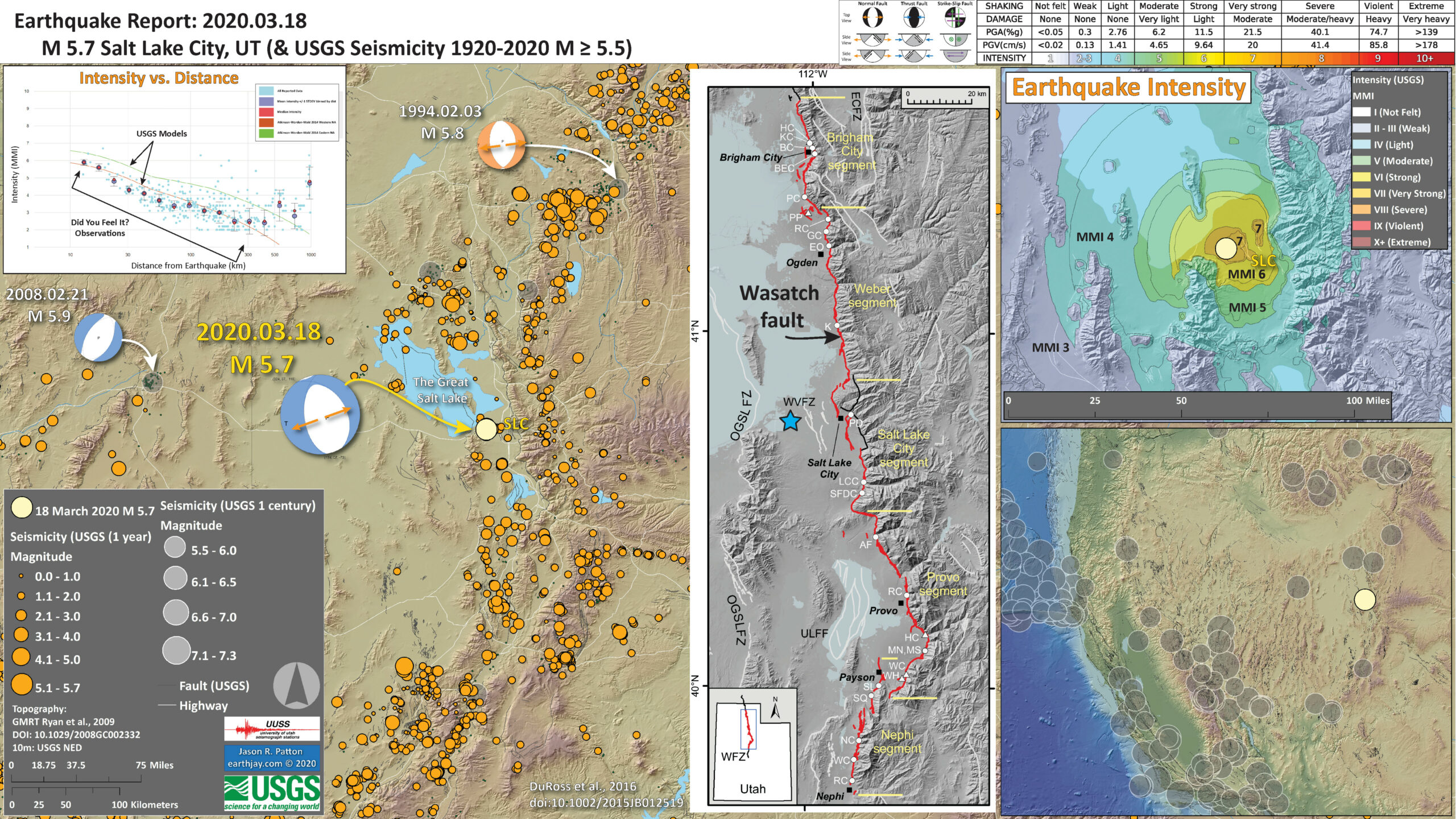
Below is my interpretive poster for this earthquake
- I plot the seismicity from the past month, with diameter representing magnitude (see legend). I include earthquake epicenters from 1919-2019 with magnitudes M ≥ 3.0 in one version.
- I plot the USGS fault plane solutions (moment tensors in blue and focal mechanisms in orange), possibly in addition to some relevant historic earthquakes.
- A review of the basic base map variations and data that I use for the interpretive posters can be found on the Earthquake Reports page.
- Some basic fundamentals of earthquake geology and plate tectonics can be found on the Earthquake Plate Tectonic Fundamentals page.
- In the lower right corner is a map of the western USA with USGS seismicity from the past century for earthquakes M 5.5+. Note all the north-south oriented lines in Nevada and Utah. These are formed by all the normal faults from the east-west extension in the basin and range.
- In the upper right corner is a map of the Salt Lake City (SLC) area. The Great Salt Lake is the large light blue bleb in the upper right. We can see the mountains to the east of SLC, the Wasatch Range. The Earthquake Intensity uses the MMI scale (the colors), read more about this here. This map represents an estimate of ground shaking from the M 5.7 based on a statistical model using the results of tens of thousands of earthquakes.
- In the upper left corner is a plot showing how these USGS models “predict” the ground shaking intensity will be relative to distance from the earthquake. These models are represented by the broan and green lines. People can fill out an online form to enter their observations and these “Did You Feel It?” observations are converted into an intensity number and these are plotted as dots in this figure.
- In the left-center is a map from DuRoss et al. (2016) that shows the Wasatch fault along the base of the Wasatch Range. Note that the fault is subdivided into different segments. We think that sometimes these different segments may rupture at different times and sometimes some of them may rupture at the same time.I placed a blue star in the location of today’s earthquake (projected onto the surface).
I include some inset figures. Some of the same figures are located in different places on the larger scale map below.
- Here is the map with 1 year’s and 1 century’s seismicity plotted.

- Two great resources for information about the tectonics of Utah are here:
- Emily Kleber fromt he Utah Geological Survey put together this excellent overview.
- Here is a Handbook for earthquakes in Utah. This is a pdf and can be printed out for the use in lesson plans for a variety of age groups. I particularly like the artwork on the cover.
- Here is a clearinghouse of photos of damage from the earthquake (h/t to Nick Graehl, my coworker, for pointing this out).
Other Report Pages
Some Relevant Discussion and Figures
- Here is the map from DuRoss et al. (2016).
- The main fault is in red. There are additional faults, like the white lines west of Salt Lake City. These are traces of the West Valley fault zone (WVFZ). Note the next mountain range to the west (left) and that there is another north-south series of faults drawn at the base of those mountains too. This is the Oquirrh Great Salt Lake fault zone, a series of west dipping faults (just like the Wasatch fault)
- The Wasatch fault is very long and notice how it is not continuous. One of the important things that we may want to know is if these all slip at the same time during an earthquake, or only some of them slip, or just one of them. This is one of the largest sources of uncertainty when it comes to estimating the seismic hazard of a region.
- The authors (and others before them) subdivided the segments and these segments are labeled on this map.

Central segments of the WFZ (red), which have evidence of repeated Holocene surface-faulting earthquakes. Circles indicate sites with data that we reanalyzed using OxCal (abbreviations shown in Table 2); triangles indicate sites where data or documentation was inadequate for reanalysis (HC, Hobble Creek; PP, Pole Patch; WC, Water Canyon; WH, Woodland Hills). Other Quaternary faults in northern Utah (white lines) include the ECFZ, East Cache fault zone; OGSLFZ, Oquirrh Great Salt Lake fault zone; ULFF, Utah Lake faults and folds; WVFZ, West Valley fault zone. Fault traces are from Black et al. [2003]. Horizontal bars mark primary segment boundaries. Inset map shows the trace of the WFZ in northern Utah and southern Idaho.
- This is a figure that shows what we think may be the way that these fault segments link (or not) through time (DuRoss et la., 2016).
- The fault line map is on top (note how North is not always “up.”). The bottom chart aligns with the fault segments (along the north south distance represented by the red dashed and dotted line in the map).
- The vertical axis is time in thousands of years ago (1950 is on the bottom and 7 thousand years ago is on top). Each blue bar represents the time that an earthquake may haven happened in the past and how those earthquakes may match the earthquake history of an adjacent segment.
- If the blue bar on one segment matches the age range for an adjacent fault, that earthquake may have involved both segments. However due to the limitation with radiocarbon, we can never really know this.

Late Holocene surface-faulting earthquakes identified at trench sites along the central WFZ. Circles with labels indicate sites with data that were reanalyzed using OxCal, and unlabeled white triangles indicate sites where data or documentation was inadequate for reanalysis. Distance is measured along simplified fault trace (dash dotted line) shown in top panel. Individual earthquake-timing probability density functions (PDFs) and mean times are derived from OxCal models for the paleoseismic sites; number in brackets is event number, where one is the youngest.
- Here is a cross section, showing us what we think may be how the faults extend beneath the ground surface. Drt, DuRoss tweeted this today.
- The Wasatch fault begins on the right, at the base of the Wasatch Mountains and dips to the west (to the left) beneath Salt Lake City.
- There are additional (antithetic) faults dipping to the east and these are called the West Valley fault zone. They are also normal faults formed from extension.
- These faults are plotted in white in the above map.
- The earthquake location is also plotted using two different information sources. According to Dr. RuRoss, these earthquakes may have happened on a previously unknown fault.

Earthquake Triggered Landslides
-
There are many different ways in which a landslide can be triggered. The first order relations behind slope failure (landslides) is that the “resisting” forces that are preventing slope failure (e.g. the strength of the bedrock or soil) are overcome by the “driving” forces that are pushing this land downwards (e.g. gravity). The ratio of resisting forces to driving forces is called the Factor of Safety (FOS). We can write this ratio like this:
- Here is a map that I put together using the data available from the USGS Earthquake Event pages. More about these models can be found here.
- The map shows liquefaction susceptibility from the M 5.7 earthquake.
- These models use empirical relations (earthquake data) between earthquake size, earthquake distance, and material properties of the Earth.
- The largest assumption is that for the Earth materials. This model uses a global model for the seismic velocity in the upper 30 meters (i.e. the Vs30). This global model basically takes the topographic slope of the ground surface and converts that to Vs30. So, the model is basically based on a slope map. This is imperfect, but works moderately well at a global scale. A model based on real Earth material data would be much much better.
FOS = Resisting Force / Driving Force
When FOS > 1, the slope is stable and when FOS < 1, the slope fails and we get a landslide. The illustration below shows these relations. Note how the slope angle α can take part in this ratio (the steeper the slope, the greater impact of the mass of the slope can contribute to driving forces). The real world is more complicated than the simplified illustration below.

Landslide ground shaking can change the Factor of Safety in several ways that might increase the driving force or decrease the resisting force. Keefer (1984) studied a global data set of earthquake triggered landslides and found that larger earthquakes trigger larger and more numerous landslides across a larger area than do smaller earthquakes.
Earthquakes can cause landslides because the seismic waves can cause the driving force to increase (the earthquake motions can “push” the land downwards), leading to a landslide. In addition, ground shaking can change the strength of these earth materials (a form of resisting force) with a process called liquefaction.
Sediment or soil strength is based upon the ability for sediment particles to push against each other without moving. This is a combination of friction and the forces exerted between these particles. This is loosely what we call the “angle of internal friction.” Liquefaction is a process by which pore pressure increases cause water to push out against the sediment particles so that they are no longer touching.
An analogy that some may be familiar with relates to a visit to the beach. When one is walking on the wet sand near the shoreline, the sand may hold the weight of our body generally pretty well. However, if we stop and vibrate our feet back and forth, this causes pore pressure to increase and we sink into the sand as the sand liquefies. Or, at least our feet sink into the sand.
Below is a diagram showing how an increase in pore pressure can push against the sediment particles so that they are not touching any more. This allows the particles to move around and this is why our feet sink in the sand in the analogy above. This is also what changes the strength of earth materials such that a landslide can be triggered.

Below is a diagram based upon a publication designed to educate the public about landslides and the processes that trigger them (USGS, 2004). Additional background information about landslide types can be found in Highland et al. (2008). There was a variety of landslide types that can be observed surrounding the earthquake region. So, this illustration can help people when they observing the landscape response to the earthquake whether they are using aerial imagery, photos in newspaper or website articles, or videos on social media. Will you be able to locate a landslide scarp or the toe of a landslide? This figure shows a rotational landslide, one where the land rotates along a curvilinear failure surface.


- 2020.03.18 M 5.7 Salt Lake City, Utah
- 2017.09.02 M 5.3 Idaho
- 2016.12.28 M 5.7 swarm Nevada
- 2014.11.05 M 4.6 swarm Nevada
Basin and Range
General Overview
Earthquake Reports
Utah
Idaho
Nevada
Social Media
— Jason "Jay" R. Patton (@patton_cascadia) March 19, 2020
This 3-D representation shows earthquake locations of the 03/18/20, Magna sequence. The largest circle is the magnitude 5.7 main shock, at a depth of about 7.5 miles (12 km), and the other circles are aftershocks that had occurred through 1:30 pm MDT.https://t.co/5YuwS7G8Rm pic.twitter.com/uPDuoiRX3l
— Utah Geological (@utahgeological) March 18, 2020
UGS geologists are on the ground documenting the geologic effects of today's earthquakes. More information will be added as our field teams continue their investigations.https://t.co/0U7ga954RD#utahearthquake pic.twitter.com/La1oJnIIhy
— Utah Geological (@utahgeological) March 19, 2020
- Frisch, W., Meschede, M., Blakey, R., 2011. Plate Tectonics, Springer-Verlag, London, 213 pp.
- Hayes, G., 2018, Slab2 – A Comprehensive Subduction Zone Geometry Model: U.S. Geological Survey data release, https://doi.org/10.5066/F7PV6JNV.
- Holt, W. E., C. Kreemer, A. J. Haines, L. Estey, C. Meertens, G. Blewitt, and D. Lavallee (2005), Project helps constrain continental dynamics and seismic hazards, Eos Trans. AGU, 86(41), 383–387, , https://doi.org/10.1029/2005EO410002. /li>
- Jessee, M.A.N., Hamburger, M. W., Allstadt, K., Wald, D. J., Robeson, S. M., Tanyas, H., et al. (2018). A global empirical model for near-real-time assessment of seismically induced landslides. Journal of Geophysical Research: Earth Surface, 123, 1835–1859. https://doi.org/10.1029/2017JF004494
- Kreemer, C., J. Haines, W. Holt, G. Blewitt, and D. Lavallee (2000), On the determination of a global strain rate model, Geophys. J. Int., 52(10), 765–770.
- Kreemer, C., W. E. Holt, and A. J. Haines (2003), An integrated global model of present-day plate motions and plate boundary deformation, Geophys. J. Int., 154(1), 8–34, , https://doi.org/10.1046/j.1365-246X.2003.01917.x.
- Kreemer, C., G. Blewitt, E.C. Klein, 2014. A geodetic plate motion and Global Strain Rate Model in Geochemistry, Geophysics, Geosystems, v. 15, p. 3849-3889, https://doi.org/10.1002/2014GC005407.
- Meyer, B., Saltus, R., Chulliat, a., 2017. EMAG2: Earth Magnetic Anomaly Grid (2-arc-minute resolution) Version 3. National Centers for Environmental Information, NOAA. Model. https://doi.org/10.7289/V5H70CVX
- Müller, R.D., Sdrolias, M., Gaina, C. and Roest, W.R., 2008, Age spreading rates and spreading asymmetry of the world’s ocean crust in Geochemistry, Geophysics, Geosystems, 9, Q04006, https://doi.org/10.1029/2007GC001743
- Pagani,M. , J. Garcia-Pelaez, R. Gee, K. Johnson, V. Poggi, R. Styron, G. Weatherill, M. Simionato, D. Viganò, L. Danciu, D. Monelli (2018). Global Earthquake Model (GEM) Seismic Hazard Map (version 2018.1 – December 2018), DOI: 10.13117/GEM-GLOBAL-SEISMIC-HAZARD-MAP-2018.1
- Silva, V ., D Amo-Oduro, A Calderon, J Dabbeek, V Despotaki, L Martins, A Rao, M Simionato, D Viganò, C Yepes, A Acevedo, N Horspool, H Crowley, K Jaiswal, M Journeay, M Pittore, 2018. Global Earthquake Model (GEM) Seismic Risk Map (version 2018.1). https://doi.org/10.13117/GEM-GLOBAL-SEISMIC-RISK-MAP-2018.1
- Zhu, J., Baise, L. G., Thompson, E. M., 2017, An Updated Geospatial Liquefaction Model for Global Application, Bulletin of the Seismological Society of America, 107, p 1365-1385, https://doi.org/0.1785/0120160198
- DuRoss, C. B., S. F. Personius, A. J. Crone, S. S. Olig, M. D. Hylland, W. R. Lund, and D. P. Schwartz (2016), Fault segmentation: New concepts from the Wasatch Fault Zone, Utah, USA, J. Geophys. Res. Solid Earth, 121, 1131–1157, doi:10.1002/2015JB012519.
References:
Basic & General References
Specific References
Return to the Earthquake Reports page.
- Sorted by Magnitude
- Sorted by Year
- Sorted by Day of the Year
- Sorted By Region