
A couple weeks ago there was a magnitude 7.4 earthquake in the Molucca Strait, Indonesia (south of the Philippines). https://earthquake.usgs.gov/earthquakes/eventpage/us6000slss/executive I am working on this report but cannot upload new images to the website until I return home. The Halmahera…

Earthquake Report: M 7.5 Guatemala
In 1976 there was a devastating earthquake in Guatemala with a magnitude of M 7.5. https://earthquake.usgs.gov/earthquakes/eventpage/usp0000ex3/executive The 2026 PATA Days (Paleoseismology, Active Tectonics, and Archeoseismology) is being held in Guatemala this year. Fifty years since the earthquake. Geologists will likely…
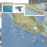
Earthquake Report: M 6.5 Acapulco, Mexico
Yesterday morning there was a M 6.5 earthquake near the coast southeast of Acapulco, Mexico. https://earthquake.usgs.gov/earthquakes/eventpage/us7000rm3k/executive Based on the earthquake mechanism and the location, I interpret this to probably be a megathrust subduction zone interface earthquake (the subduction zone fault…
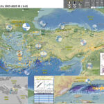
Earthquake Report: M 6.2 Turkey
Here I present a poster for the M 6.2 earthquake in the Marmara Sea, northwest of Turkey. https://earthquake.usgs.gov/earthquakes/eventpage/us7000pufs/executive This earthquake slipped along the North Anatolia fault (NAF), a right-lateral strike-slip fault that trends along the northern part of Turkey. Most…

Earthquake Report: M 7.4 Kamchatka
Here I present a poster for the M 7.4 Kamchatka, Russia Earthquake. https://earthquake.usgs.gov/earthquakes/eventpage/us7000qdyl/executive This earthquake slipped along the megathrust subduction zone in the region that slipped during a M 8.8-9.0 earthquake in 1952. I don’t always have the time to…
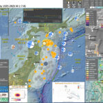
Earthquake Report: M 7.6 Japan
Here I present a poster for the M 7.6 Aomori Prefecture, Japan Earthquake. https://earthquake.usgs.gov/earthquakes/eventpage/us6000rtdt/executive This earthquake slipped along the megathrust subduction zone just north of the region that slipped during the 2011 Tohoku-oki earthquake. There was a small tsunami observed…
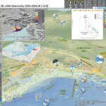
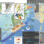
Earthquake Report: M 7.0 Yukon Territory/Alaska
Here I present a poster for the M 7.0 Hubbard Glacier Earthquake in Yukon Territory/Alaska. https://earthquake.usgs.gov/earthquakes/eventpage/us6000rsy1/executive This earthquake slipped along a fault that connects the Queen Charlotte/Fairweather fault system with the Totschunda fault (that slipped in 2002). This fault is…
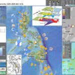
Earthquake Report: M 6.9 Philippines
Here I present a poster for the M 6.9 Hubbard Glacier Earthquake in Yukon Territory/Alaska. https://earthquake.usgs.gov/earthquakes/eventpage/us6000rdrz/executive This earthquake slipped along a fault that may be related to the Philippine fault (a strike-slip fault. The mechanism is strike-slip and because of…
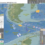
Earthquake Report: M 7.5 Drake Passage
It looks like I did not write up much for this earthquake initially. Here is the USGS website for this (now) M 7.6 earthquake in the Drake Passage: https://earthquake.usgs.gov/earthquakes/eventpage/us6000rgf4/executive This appears related to an earlier earthquake in the region. But…
Earthquake Report: M 8.8 Kamchatka
Earlier this week, I was wrapping up some work, getting ready to go home to work some more (a pending deadline!). There was a magnitude M 4.5 earthquake offshore. However, it was too far offshore to meet criteria for reporting,…