
There was a M = 6.8 earthquake along a transform fault connecting segments of the Mid Atlantic Ridge recently. (now an M 6.7)
https://earthquake.usgs.gov/earthquakes/eventpage/us1000hpim/executive
The Mid Atlantic Ridge is an extensional plate boundary called an oceanic spreading ridge. Oceanic crust is formed along these types of plate boundaries.
Transform faults are faults that move side-by-side (i.e. strike-slip faults) that offset spreading ridges. Learn more about different types of faults in the geologic fundamentals section below.
The Atlantic Ocean is known for the spreading center, Mid Atlantic Ridge (MAR), which was probably born in the mid Cretaceous Period, about 130 million years ago. We use the age of the oceanic crust at the eastern and western margins of the Atlantic Ocean as a basis for this interpretation.
The Mid Atlantic Ridge also splits apart the island of Iceland, which also overlies a volcanic hot spot. I have always wanted to visit Iceland to see the rocks get older as I might travel east or west from the middle of Iceland.
North of Iceland, the MAR is offset by many small and several large transform faults. The largest transform fault north of Iceland is called the Jan Mayen fracture zone, which is the location for the 2018.11.08 M = 6.8 earthquake.
Below is my interpretive poster for this earthquake
I plot the seismicity from the past month, with color representing depth and diameter representing magnitude (see legend). I include earthquake epicenters from 1918-2018 with magnitudes M ≥ 4.5 in one version.
I plot the USGS fault plane solutions (moment tensors in blue and focal mechanisms in orange), possibly in addition to some relevant historic earthquakes. I also include the IPGP focal mechanism as that was available before the USGS moment tensor was available (I included it in my initial poster).
- I placed a moment tensor / focal mechanism legend on the poster. There is more material from the USGS web sites about moment tensors and focal mechanisms (the beach ball symbols). Both moment tensors and focal mechanisms are solutions to seismologic data that reveal two possible interpretations for fault orientation and sense of motion. One must use other information, like the regional tectonics, to interpret which of the two possibilities is more likely.
- I also include the shaking intensity contours on the map. These use the Modified Mercalli Intensity Scale (MMI; see the legend on the map). This is based upon a computer model estimate of ground motions, different from the “Did You Feel It?” estimate of ground motions that is actually based on real observations. The MMI is a qualitative measure of shaking intensity. More on the MMI scale can be found here and here. This is based upon a computer model estimate of ground motions, different from the “Did You Feel It?” estimate of ground motions that is actually based on real observations.
- I include the slab 2.0 contours plotted (Hayes, 2018), which are contours that represent the depth to the subduction zone fault. These are mostly based upon seismicity. The depths of the earthquakes have considerable error and do not all occur along the subduction zone faults, so these slab contours are simply the best estimate for the location of the fault.li>
- In the map below, I include a transparent overlay of the magnetic anomaly data from EMAG2 (Meyer et al., 2017). As oceanic crust is formed, it inherits the magnetic field at the time. At different points through time, the magnetic polarity (north vs. south) flips, the north pole becomes the south pole. These changes in polarity can be seen when measuring the magnetic field above oceanic plates. This is one of the fundamental evidences for plate spreading at oceanic spreading ridges (like the Mid Atlantic Ridge).
- Regions with magnetic fields aligned like today’s magnetic polarity are colored red in the EMAG2 data, while reversed polarity regions are colored blue. Regions of intermediate magnetic field are colored light purple.
- We can see the roughly north-south trends of these red and blue stripes. These lines are parallel to the ocean spreading ridges from where they were formed.
Magnetic Anomalies
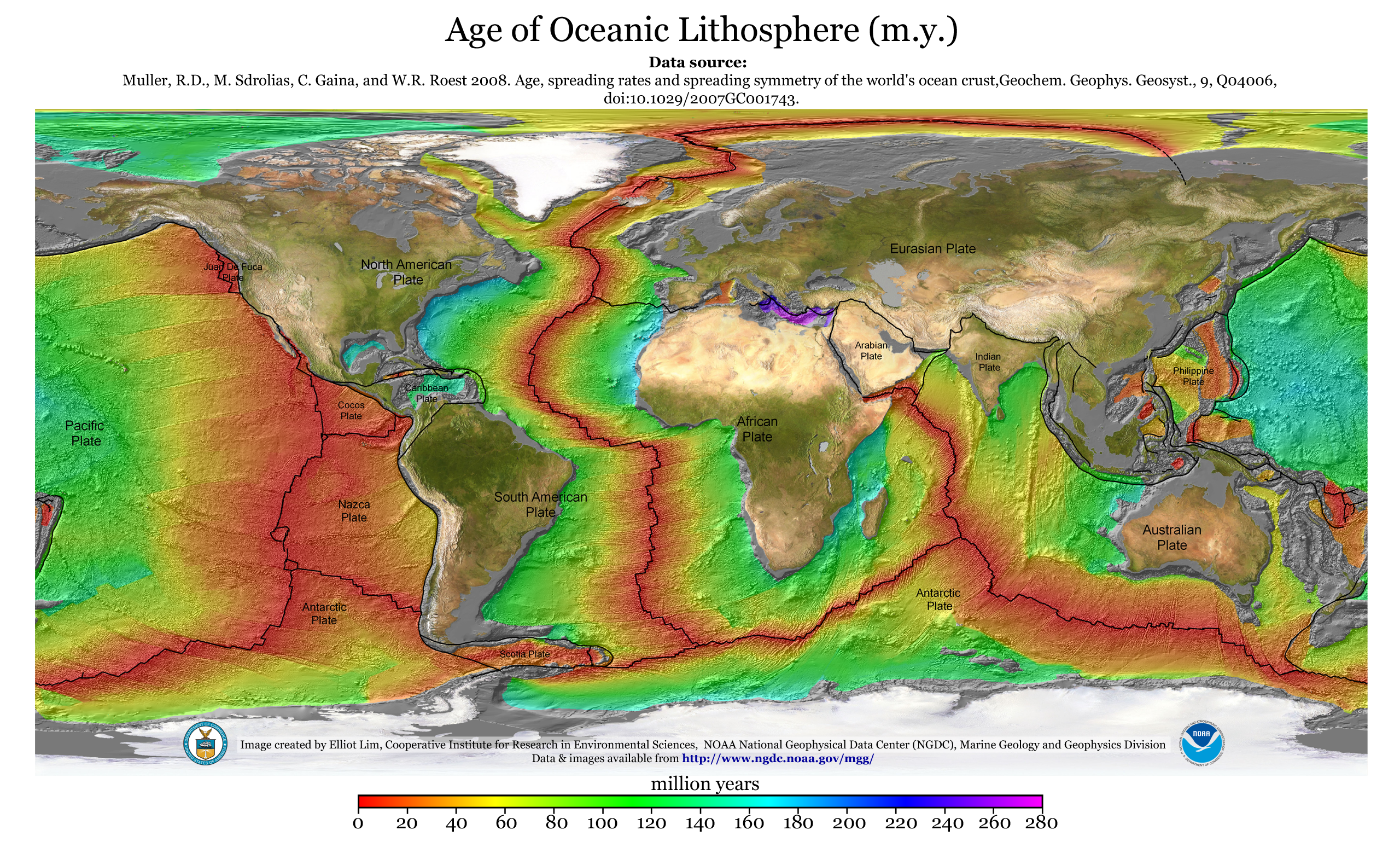
- In the map below, I include a transparent overlay of the age of the oceanic crust data from Agegrid V 3 (Müller et al., 2008).
- Because oceanic crust is formed at oceanic spreading ridges, the age of oceanic crust is youngest at these spreading ridges. The youngest crust is red and older crust is yellow (see legend at the top of this poster).
Age of Oceanic Lithosphere
- In the upper right corner is a plate tectonic map from Le Breton (et al., 2012). This map shows the configuration of the Mid Atlantic Ridge (MAR) and shows their interpretation about how this spreading center is divided into segments separated by transform faults. I placed a red star in the general location of the M = 6.8 earthquake.
- In the upper left corner is a map showing the isochrons (lines of each age for the crust) as summarized by Gaina et al. (2017). Isochrons are displayed with color relative to age.
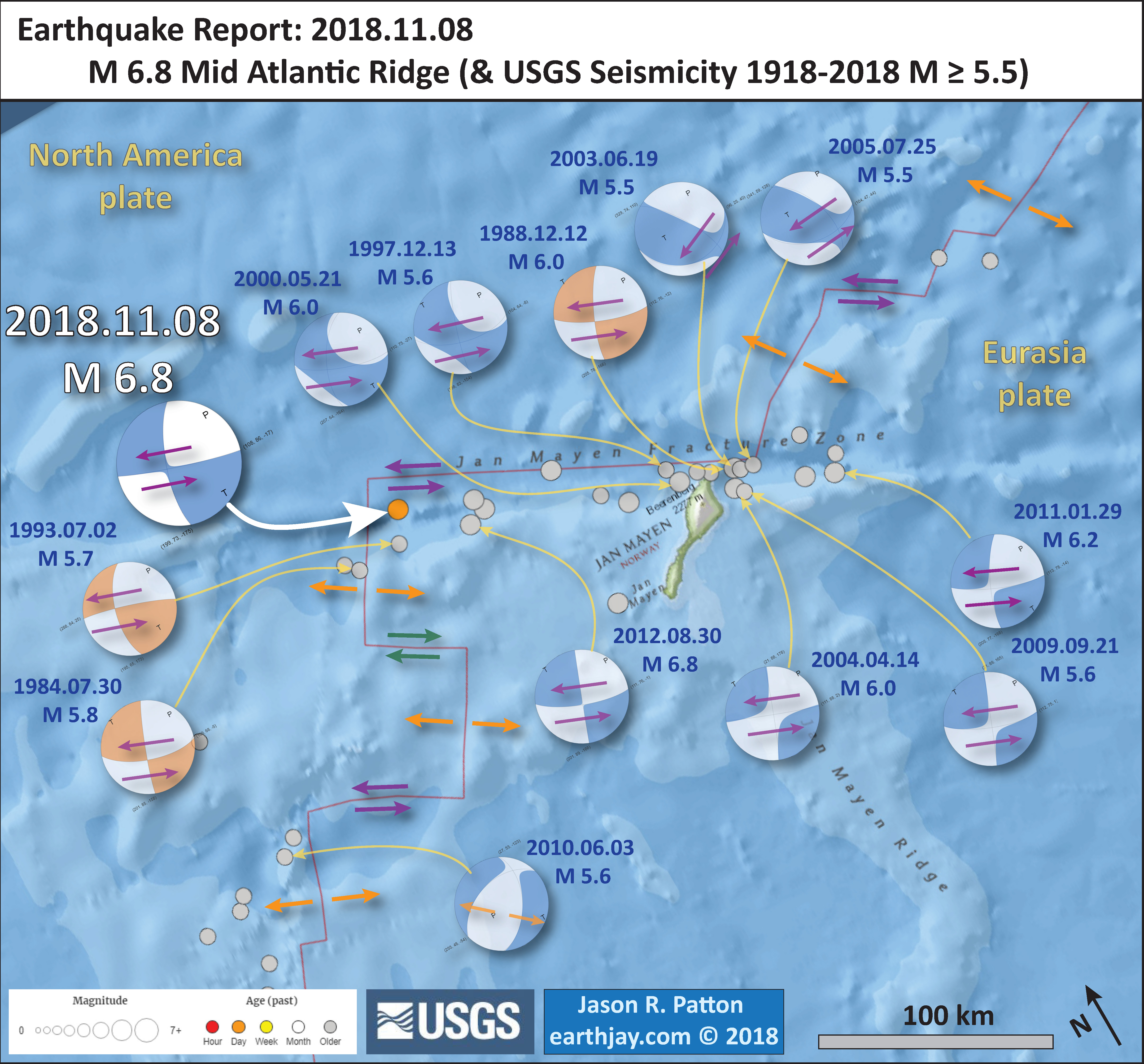
- In the lower right corner is a larger scale map zoomed into the Jan Mayen fracture zone at the MAR. I placed existing USGS fault mechanisms (blue = moment tensor, orange = focal mechanism) for earthquakes with magnitudes M ≥ 5.5.
- In the lower left corner is a map from the Temblor.net app. This map shows the seismic hazard from the GEAR model (Bird et al., 2012). Seismicity is shown as colored circles. The red dot is the M = 6.8 epicenter, which lies in a region that is forecast to have an earthquake of magnitude M = 6.25-6.5 in someone’s lifetime.
I include some inset figures. Some of the same figures are located in different places on the larger scale map below.
- Here is the map with a month’s seismicity plotted.

- Here is the map with a century’s seismicity plotted.
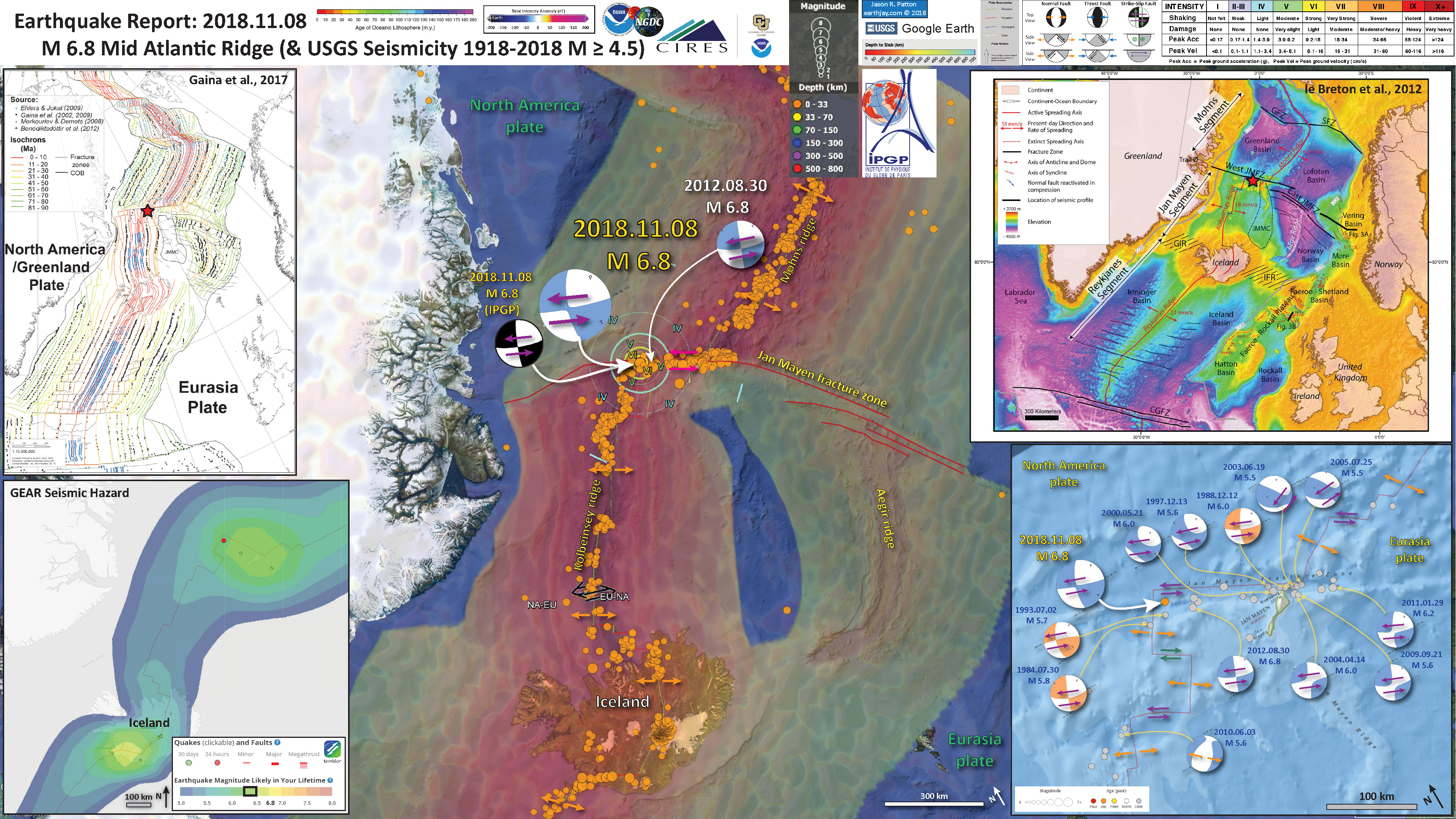
- Here is the large scale map showing earthquake mechanisms for historic earthquakes in the region. Note how they mostly behave well (are almost perfectly aligned with the Jan Mayen fracture zone). There are a few exceptions, including an extensional earthquake possibly associated with extension on the MAR (2010.06.03 M = 5.6). Also, 2 earthquakes (2003.06.19 and 2005.07.25) are show oblique slip (not pure strike-slip as they have an amount of compressional motion) near the intersection of the fracture zone and the MAR.
Some Relevant Discussion and Figures
- Here is a map that shows the ace of the oceanic lithosphere for the entire Earth.
- Here is the tectonic map from Le Breton et al. (2012). Depth to the seafloor is shown in color. Note the spreading rates in red. Note how the MAR is offset by the Jan Mayen fracture zone, as well as the smaller unnamed fracture zones.
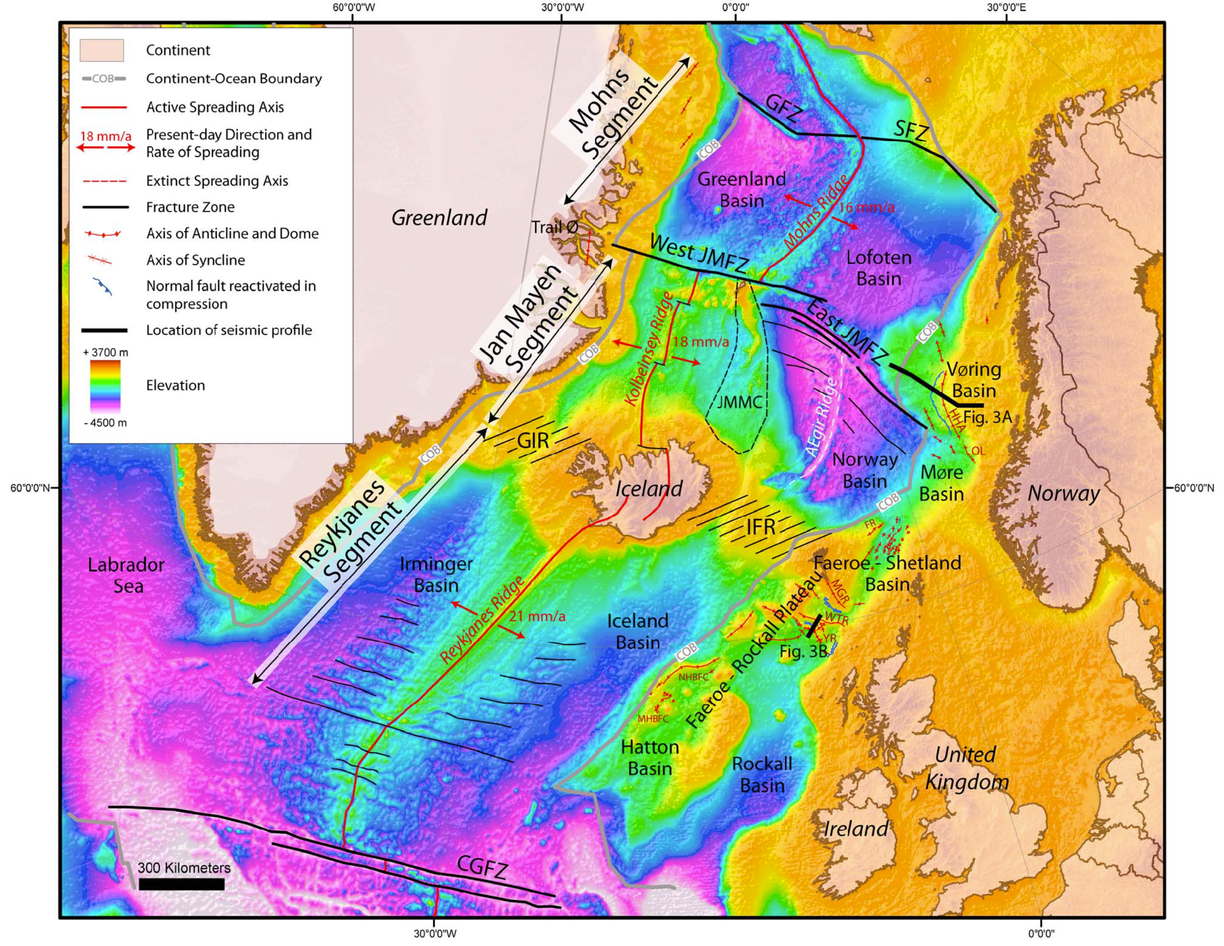
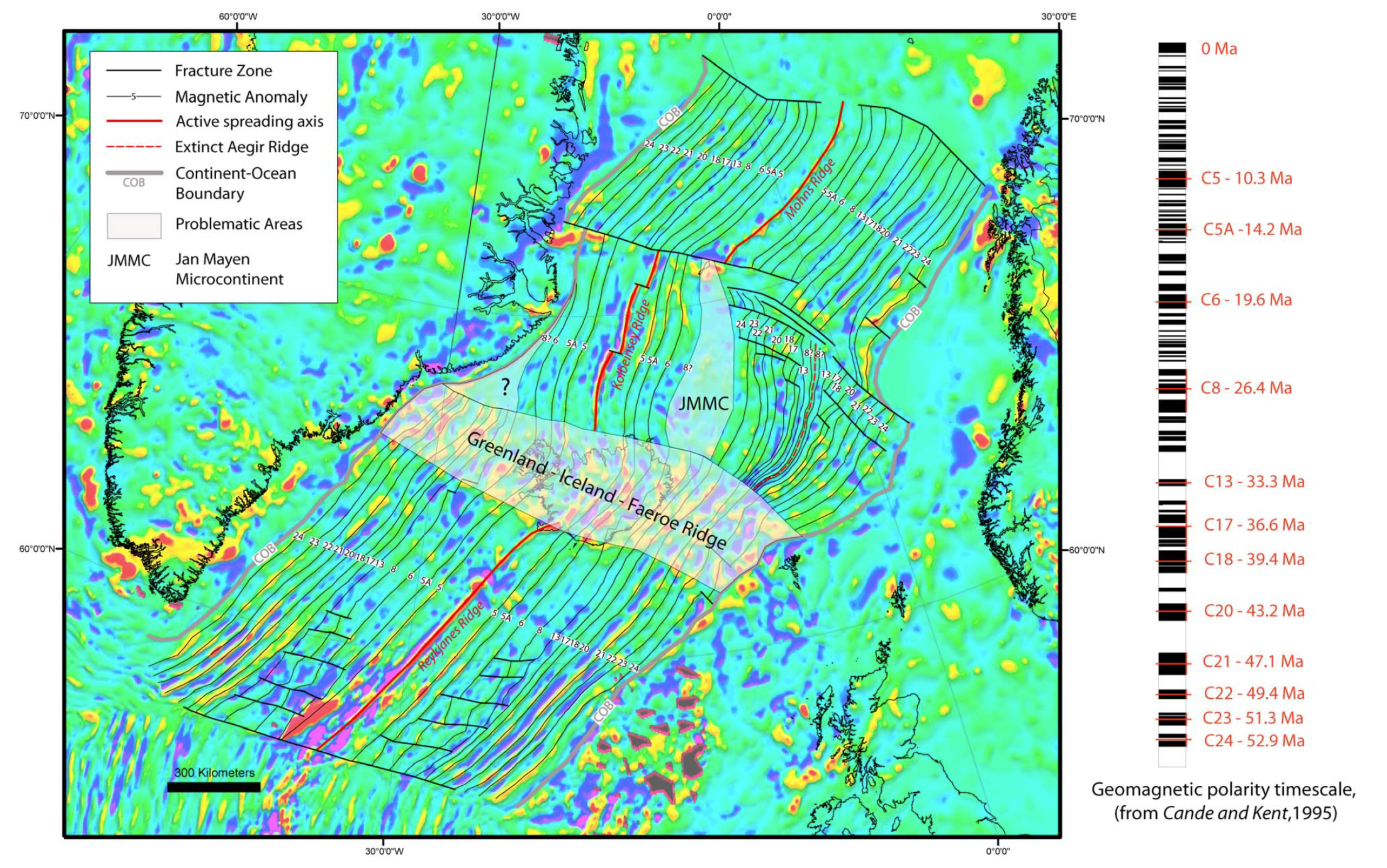
Principal tectonic features of the NE Atlantic Ocean on a bathymetric and topographic map (ETOPO1). Compressional structures (folds and reverse faults) on the NE Atlantic Continental Margin are from Doré et al. [2008], Johnson et al. [2005], Hamann et al. [2005], Price et al. [1997] and Tuitt et al. [2010]. Present-day spreading rates along Reykjavik, Kolbeinsey and Mohns Ridges are from Mosar et al. [2002]. Continent-ocean boundaries of Europe and Greenland are from Gaina et al. [2009] and Olesen et al. [2007]. Black thick lines indicate seismic profiles of Figure 3. Abbreviations (north to south): GFZ, Greenland Fracture Zone; SFZ, Senja Fracture Zone; JMFZ, Jan Mayen Fracture Zone (west and east); JMMC, Jan Mayen Microcontinent; HHA, Helland Hansen Arch; OL, Ormen Lange Dome; FR, Fugløy Ridge; GIR, Greenland-Iceland Ridge; IFR: Iceland-Faeroe Ridge; MGR, Munkagrunnar Ridge; WTR, Wyville Thomson Ridge; YR, Ymir Ridge; NHBFC, North Hatton Bank Fold Complex; MHBFC, Mid-Hatton Bank Fold Complex; CGFZ, Charlie Gibbs Fracture Zone. Map
projection is Universal Transverse Mercator (UTM, WGS 1984, zone 27N).
- This is a fantastic figure that shows the isochrons on either side of the MAR in this region (Le Breton et al., 2012). Isochrons are lines of equal age, based on magnetic anomaly mapping and numerical ages from rock samples collected from the oceanic crust.The geomagnetic time scale is shown at the right. “Chrons” are numbered with their numerical ages in millions of years (Ma). These chron numbers are also on the map, showing the chron number for each isochron. For some reason I want to watch the film Tron right now.
Map of magnetic anomalies, NE Atlantic Ocean. Background image is recent model EMAG2 of crustal magnetic anomalies [Maus et al., 2009]. Ages of magnetic anomalies are from Cande and Kent [1995]. Map projection is Universal Transverse Mercator (UTM, WGS 1984, zone 27N).
- This map shows their reconstruction of the fracture zones, MAR, and the Iceland Hot Spot for the Tertiary to present (Le Breton et al., 2012).
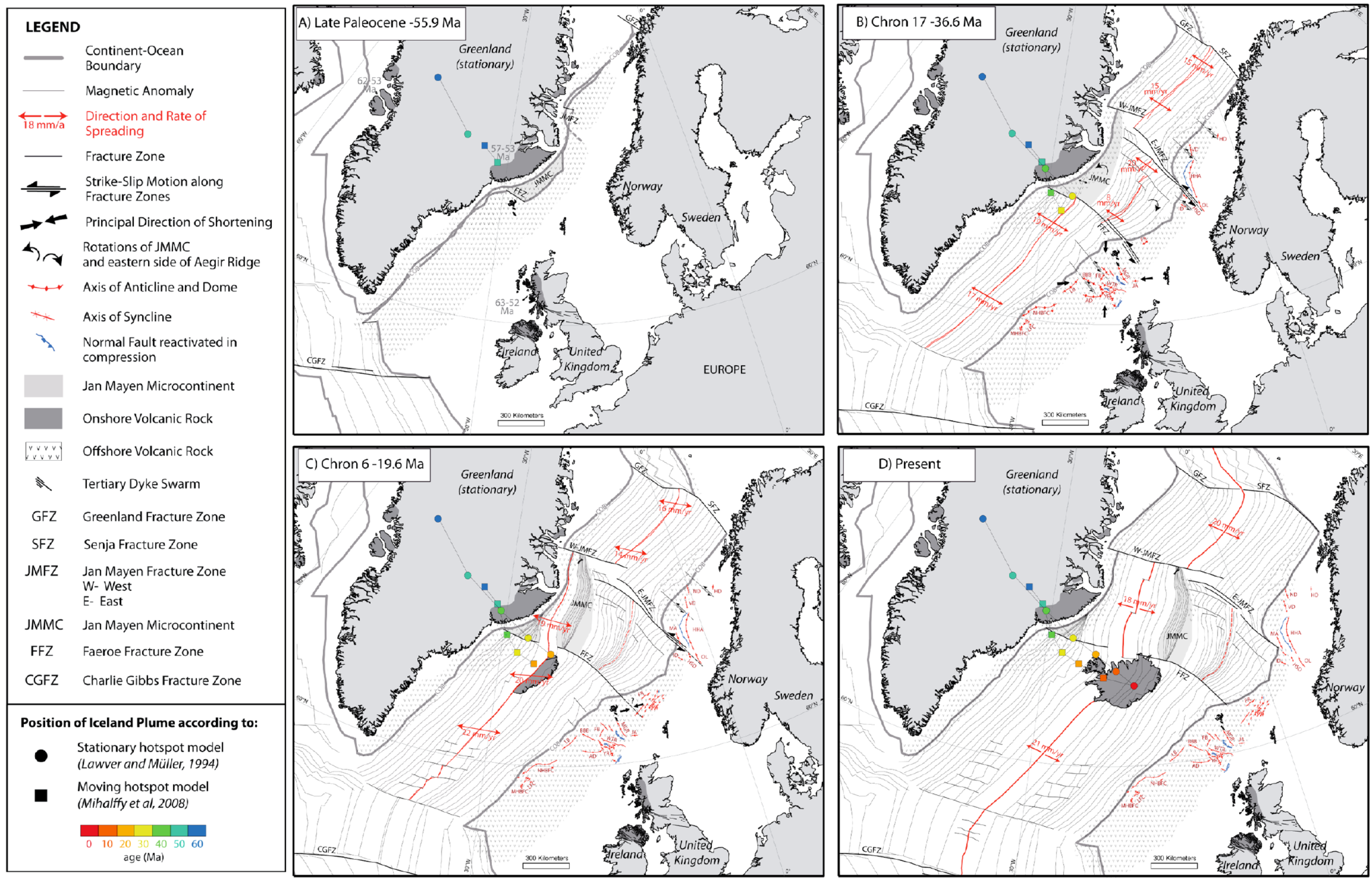
Positions relative to stationary Greenland plate of Europe, Jan Mayen Microcontinent (JMMC) and Iceland Mantle Plume at intervals of 10 Myr, according to stationary hot spot model of Lawver and Müller [1994] and moving hot spot model of Mihalffy et al. [2008]. Timing is (a) late Paleocene, 55.9 Ma; (b) late Eocene, 36.6 Ma ; (c) early Miocene, 19.6 Ma; and (d) present. (more info is in the original figure caption)
- Here is the Gaina et al. (2017 a) isochron map for this region of the north Atlantic Ocean. Below are also some great summary figures that show a series of geophysical data from their work in the region (Gaina et al., 2017 b).
- On the left is a free air gravity map (Gaina et al., 2017 b). This is a gravity map after the “free-air” correction has been made (that corrects for the elevation that the gravity data were observed).
- On the right is the isostatic gravity anomaly map. This is a gravity map that shows the results of correcting the gravity data for the variable density of materials in the earth’s crust and mantle.
- On the left is the magnetic anomaly map (Gaina et al., 2017 b)
- On the right is the sediment thickness map.
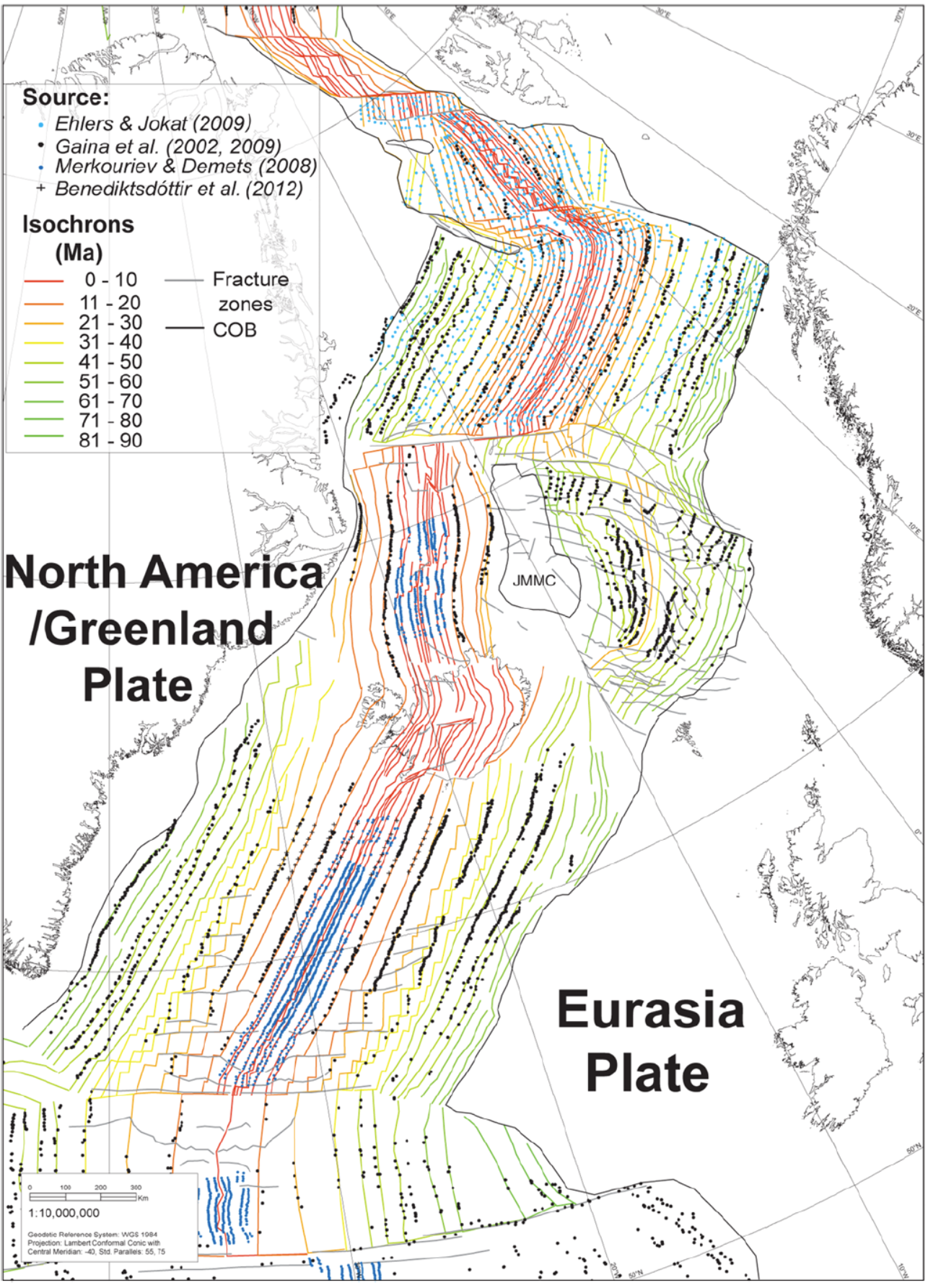
Magnetic anomaly and fracture zone identifications and interpreted isochrons.
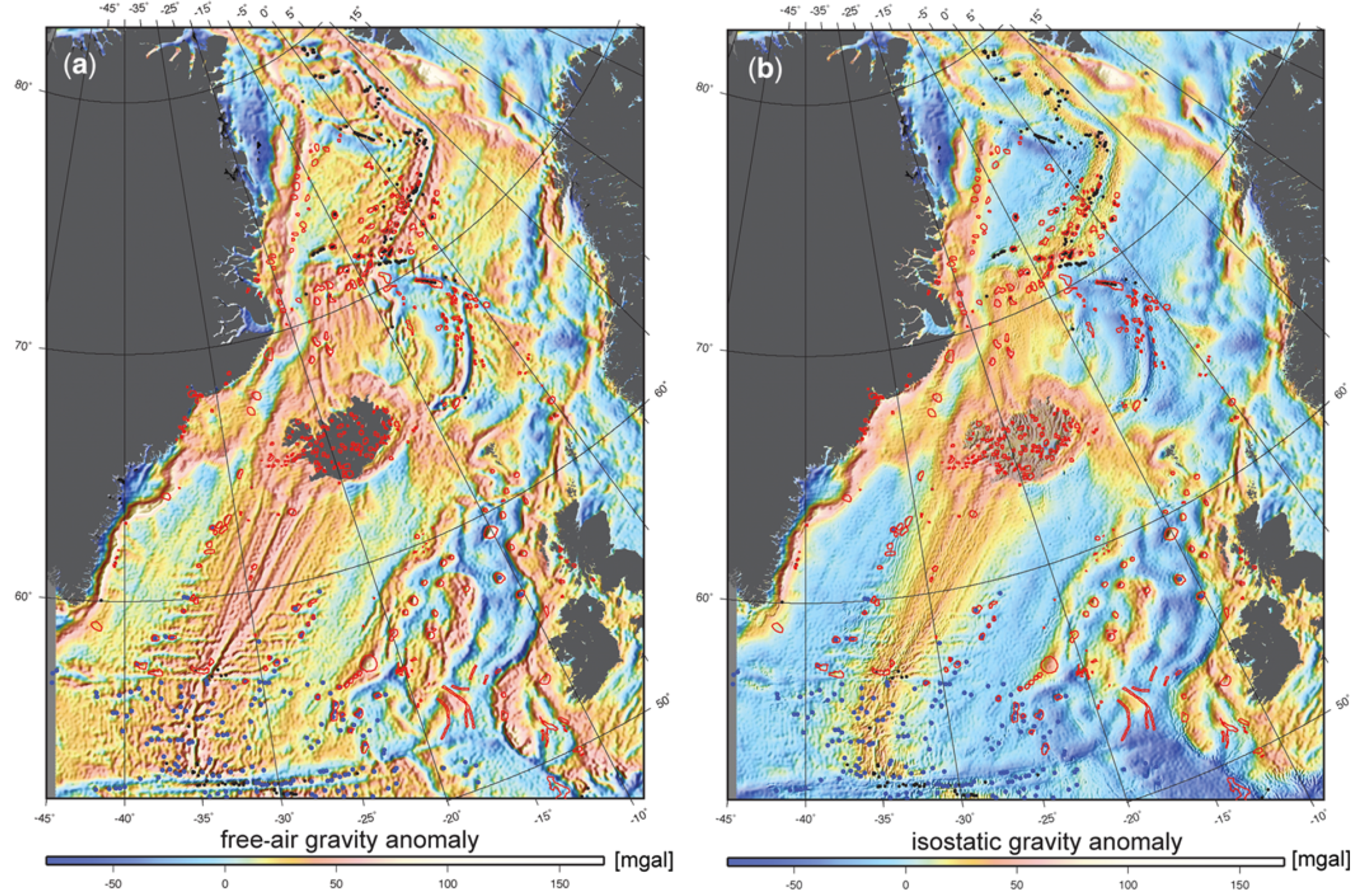
(a) Free-air gravity (DTU10: Andersen 2010); (b) isostatic gravity anomaly (this was computed using the Airy–Heiskanen model, where the compensation is accomplished by variations in thickness of the constant density layers: the root is calculated using the ETOPO1 topography and bathymetry: Haase et al., this volume, in press);

magnetic anomaly (Nasuti & Olesen 2014; Gaina et al., this volume, in review); and (d) sediment thickness (Funck et al. 2014). Distribution of volcanic edifices as in Figure 1. Dark grey lines indicate the active and extinct plate boundaries
- This is a really cool map that shows how the MAR extends further into the Arctic Ocean. Color represents depth to the seafloor (Mjelde et al., 2008).

Location map of the North Atlantic and Arctic. ETOPO-2 shaded relief bathymetry and topography are based on data from Sandwell & Smith (1997). (more detail is found in the original figure caption)
Geologic Fundamentals
- For more on the graphical representation of moment tensors and focal mechnisms, check this IRIS video out:
- Here is a fantastic infographic from Frisch et al. (2011). This figure shows some examples of earthquakes in different plate tectonic settings, and what their fault plane solutions are. There is a cross section showing these focal mechanisms for a thrust or reverse earthquake. The upper right corner includes my favorite figure of all time. This shows the first motion (up or down) for each of the four quadrants. This figure also shows how the amplitude of the seismic waves are greatest (generally) in the middle of the quadrant and decrease to zero at the nodal planes (the boundary of each quadrant).

- Here is another way to look at these beach balls.
The two beach balls show the stike-slip fault motions for the M6.4 (left) and M6.0 (right) earthquakes. Helena Buurman's primer on reading those symbols is here. pic.twitter.com/aWrrb8I9tj
— AK Earthquake Center (@AKearthquake) August 15, 2018
- There are three types of earthquakes, strike-slip, compressional (reverse or thrust, depending upon the dip of the fault), and extensional (normal). Here is are some animations of these three types of earthquake faults. The following three animations are from IRIS.
Strike Slip:
Compressional:
Extensional:
- This is an image from the USGS that shows how, when an oceanic plate moves over a hotspot, the volcanoes formed over the hotspot form a series of volcanoes that increase in age in the direction of plate motion. The presumption is that the hotspot is stable and stays in one location. Torsvik et al. (2017) use various methods to evaluate why this is a false presumption for the Hawaii Hotspot.
- Here is a map from Torsvik et al. (2017) that shows the age of volcanic rocks at different locations along the Hawaii-Emperor Seamount Chain.

A cutaway view along the Hawaiian island chain showing the inferred mantle plume that has fed the Hawaiian hot spot on the overriding Pacific Plate. The geologic ages of the oldest volcano on each island (Ma = millions of years ago) are progressively older to the northwest, consistent with the hot spot model for the origin of the Hawaiian Ridge-Emperor Seamount Chain. (Modified from image of Joel E. Robinson, USGS, in “This Dynamic Planet” map of Simkin and others, 2006.)

Hawaiian-Emperor Chain. White dots are the locations of radiometrically dated seamounts, atolls and islands, based on compilations of Doubrovine et al. and O’Connor et al. Features encircled with larger white circles are discussed in the text and Fig. 2. Marine gravity anomaly map is from Sandwell and Smith.
- 2018.11.08 M 6.8 Mid Atlantic Ridge (Jan Mayen fracture zone)
- 2017.08.18 M 6.6 Mid Atlantic Ridge (Chan fracture zone)
- 2016.08.30 M 7.1 Mid Atlantic Ridge
- 2015.06.18 M 7.0 Mid Atlantic Ridge
- 2015.05.24 M 6.3 Mid Atlantic Ridge
- 2015.02.13 M 7.1 Mid Atlantic Ridge
Atlantic
Earthquake Reports
Social Media
Mw=6.8, JAN MAYEN ISLAND REGION (Depth: 21 km), 2018/11/09 01:49:40 UTC – Full details here: https://t.co/gUvvmkw24e pic.twitter.com/DdtvaBq2Fc
— Earthquakes (@geoscope_ipgp) November 9, 2018
Using a low pass filter highlights the Surface waves sweeping across the UK. You can clearly see that the lowest frequency components (widest spacing between wiggles) arrive before higher frequency (closer spaced wiggles) components. Scientists call this effect dispersion. pic.twitter.com/eRcZ37TtsQ
— BGS schoolseismology (@Schoolseismo) November 9, 2018
- Bird, P., Jackson, D. D., Kagan, Y. Y., Kreemer, C., and Stein, R. S., 2015. GEAR1: A global earthquake activity rate model constructed from geodetic strain rates and smoothed seismicity, Bull. Seismol. Soc. Am., v. 105, no. 5, p. 2538–2554, DOI: 10.1785/0120150058
- Gaina, C., Nasuti, A., Kimbell, G.S., and Blishchke, A., 2017 a. Break-up and seafloor spreading domains in the NE Atlantic in Peron-Pinvidic, G., Hopper, J. R., Stoker, M. S., Gaina, C., Doornenbal, J. C., Funck, T. & Arting, U. E. (eds) 2017. The NE Atlantic Region: A Reappraisal of Crustal Structure, Tectonostratigraphy and Magmatic Evolution. Geological Society, London, Special Publications, 447, 393–417. https://doi.org/10.1144/SP447.12
- Gaina, C., Blischke, A., Geissler, W.H., Kimbell, G.S., and Erlendsson, O., 2017 b. Seamounts and oceanic igneous features in the NE Atlantic: a link between plate motions and mantle dynamics in the NE Atlantic in Peron-Pinvidic, G., Hopper, J. R., Stoker, M. S., Gaina, C., Doornenbal, J. C., Funck, T. & Arting, U. E. (eds) 2017. The NE Atlantic Region: A Reappraisal of Crustal Structure, Tectonostratigraphy and Magmatic Evolution. Geological Society, London, Special Publications, 447, 393–417. https://doi.org/10.1144/SP447.12
- Le Breton, E., P. R. Cobbold, O. Dauteuil, and G. Lewis (2012), Variations in amount and direction of seafloor spreading along the northeast Atlantic Ocean and resulting deformation of the continental margin of northwest Europe, Tectonics, 31, TC5006, doi:10.1029/2011TC003087.
- Meyer, B., Saltus, R., Chulliat, a., 2017. EMAG2: Earth Magnetic Anomaly Grid (2-arc-minute resolution) Version 3. National Centers for Environmental Information, NOAA. Model. doi:10.7289/V5H70CVX
- Müller, R.D., Sdrolias, M., Gaina, C. and Roest, W.R., 2008, Age spreading rates and spreading asymmetry of the world’s ocean crust in Geochemistry, Geophysics, Geosystems, 9, Q04006, doi:10.1029/2007GC001743
References:
Return to the Earthquake Reports page.