Earthquake Report: Chiapas Earthquake Update #2

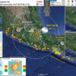
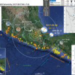
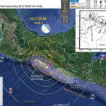
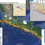
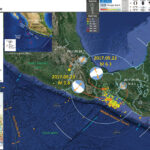
Well, we had a really interesting earthquake today. There was a M 6.1 earthquake in the North America plate (NAP) to the north of the sequence offshore of Chiapas, with the M 8.1 mainshock. Here is the USGS website for the M 6.1 earthquake. There was also an M 5.8 earthquake that was a more typical aftershock (USGS website).

Why is this earthquake interesting? It is outside the region of aftershocks from the M 8.1 earthquake and it is in the upper plate (the NAP). This is not altogether groundbreaking (pardon the pun) as there are many examples of earthquakes in one plate triggering earthquakes in other plates. For example, the recent sequence just to the south of the M 8.1 sequence (which may have led partly to the M 8.1 earthquake).

This earthquake also triggered (sorry for the pun, another one) a debate about the difference between triggered earthquakes and aftershocks. This discussion is largely semantic and does not really matter from a natural hazards perspective. The rocks behave to physics, not how we classify them. So, we don’t need to get caught up in this lexicon (as long as we all have a general understanding of what is happening). In the classic sense, I interpret this M 6.1 (and the few nearby earthquakes) to be triggered, but they are in the region that may have an increased coulomb stress.

Below is my interpretive poster for this earthquake

I plot the seismicity from the past month, with color representing depth and diameter representing magnitude (see legend). I also include USGS epicenters from 1917-2017 for magnitudes M ≥ 8.0. I include fault plane solutions for the 1985 and 1995 earthquakes (along with the MMI contours for those earthquakes, see below for a discussion of MMI contours).

  • I placed a moment tensor / focal mechanism legend on the poster. There is more material from the USGS web sites about moment tensors and focal mechanisms (the beach ball symbols). Both moment tensors and focal mechanisms are solutions to seismologic data that reveal two possible interpretations for fault orientation and sense of motion. One must use other information, like the regional tectonics, to interpret which of the two possibilities is more likely.
  • I also include the shaking intensity contours on the map. These use the Modified Mercalli Intensity Scale (MMI; see the legend on the map). This is based upon a computer model estimate of ground motions, different from the “Did You Feel It?” estimate of ground motions that is actually based on real observations. The MMI is a qualitative measure of shaking intensity. More on the MMI scale can be found here and here. This is based upon a computer model estimate of ground motions, different from the “Did You Feel It?” estimate of ground motions that is actually based on real observations.
  • I include the slab contours plotted (Hayes et al., 2012), which are contours that represent the depth to the subduction zone fault. These are mostly based upon seismicity. The depths of the earthquakes have considerable error and do not all occur along the subduction zone faults, so these slab contours are simply the best estimate for the location of the fault.

    I include some inset figures in the poster.

  • In the left center I include a generalized plate tectonic map from Wikimedia Creative Commons here.
  • In the lower left corner I include a map from Dr. Jascha Polet. Dr. Polet plots focal mechanisms for historic earthquakes. Dr. Polet notes the M 8.1, M7.1, M 6.1, and M 5.8 earthquakes too. Purple dots are epicenters after the M 8.1 earthquake and black dots are SSN (the Mexico seismic network data).
  • In the upper right corner is a map and cross section from Dr. Gavin Hayes. The upper cross section, oriented perpendicular to the subduction zone fault, shows focal mechanisms. Note how the M 8.1 (large green symbol) is in the downgoing Cocos plate and the M 6,.1 (small red symbol at about 300 km) is in the North America plate.
  • In the upper left corner is a figure Dr. Hayes also prepared. This shows the change in static coulomb stress associated with the M 8.1 earthquake. Tremblor prepared this analysis and I presented that in the M 7.1 earthquake report here. Basically, areas of warm color show an increased stress and regions of cool color show a decreased stress. So, areas in warm color are more likely to trigger an earthquake. Though this is a simple run as different faults can respond differently.


  • Here is the initial report poster as presented in my initial Earthquake Report here.

  • Here is the update #1 report poster as presented in my initial Earthquake Report here.

  • Here is the update #1 report poster for the M 7.1 Puebla, Mexico earthquake (which shows the coulomb stress modeling from Tremblor).

  • Here is Dr. Polet’s tweet of this map.
  • AND an updated map and cross section.
  • Here is Dr. Hayes’ tweet of his map and cross section.
  • Here is Dr. Hayes’ tweet of his static coulomb change map.
  • The discussion about what is a triggered earthquake and what is an aftershock, as I mentioned above, is the topic of discussion between experts in the field. The debate will probably be enduring for a quite a while, especially since classification systems are a social construct and have no real basis in reality (or physics). Classification systems are an excellent example of how science is subjective (science is fundamentally subjective, but that is a longer discussion, read some Karl Popper for more insight). This discussion led me to a web post following the 2011 Christchurch earthquake sequence. Here is a website with one view on this debate, prepared by Dr. Chris Rowan. I present two of their figures below.


References:

  • Benz, H.M., Dart, R.L., Villaseñor, Antonio, Hayes, G.P., Tarr, A.C., Furlong, K.P., and Rhea, Susan, 2011 a. Seismicity of the Earth 1900–2010 Mexico and vicinity: U.S. Geological Survey Open-File Report 2010–1083-F, scale 1:8,000,000.
  • Benz, H.M., Tarr, A.C., Hayes, G.P., Villaseñor, Antonio, Furlong, K.P., Dart, R.L., and Rhea, Susan, 2011 b. Seismicity of the Earth 1900–2010 Caribbean plate and vicinity: U.S. Geological Survey Open-File Report 2010–1083-A, scale 1:8,000,000.
  • Franco, A., C. Lasserre H. Lyon-Caen V. Kostoglodov E. Molina M. Guzman-Speziale D. Monterosso V. Robles C. Figueroa W. Amaya E. Barrier L. Chiquin S. Moran O. Flores J. Romero J. A. Santiago M. Manea V. C. Manea, 2012. Fault kinematics in northern Central America and coupling along the subduction interface of the Cocos Plate, from GPS data in Chiapas (Mexico), Guatemala and El Salvador in Geophysical Journal International., v. 189, no. 3, p. 1223-1236. DOI: https://doi.org/10.1111/j.1365-246X.2012.05390.x
  • Franco, S.I., Kostoglodov, V., Larson, K.M., Manea, V.C>, Manea, M., and Santiago, J.A., 2005. Propagation of the 2001–2002 silent earthquake and interplate coupling in the Oaxaca subduction zone, Mexico in Earth Planets Space, v. 57., p. 973-985.
  • Garcia-Casco, A., Projenza, J.A., Iturralde-Vinent, M.A., 2011. Subduction Zones of the Caribbean: the sedimentary, magmatic, metamorphic and ore-deposit records UNESCO/iugs igcp Project 546 Subduction Zones of the Caribbean in Geologica Acta, v. 9, no., 3-4, p. 217-224
  • Hayes, G. P., D. J. Wald, and R. L. Johnson, 2012. Slab1.0: A three-dimensional model of global subduction zone geometries, J. Geophys. Res., 117, B01302, doi:10.1029/2011JB008524.
  • Lay et al., 2011. Outer trench-slope faulting and the 2011 Mw 9.0 off the Pacific coast of Tohoku Earthquake in Earth Planets Space, v. 63, p. 713-718.
  • Manea, M., and Manea, V.C., 2014. On the origin of El Chichón volcano and subduction of Tehuantepec Ridge: A geodynamical perspective in JGVR, v. 175, p. 459-471.
  • Mann, P., 2007, Overview of the tectonic history of northern Central America, in Mann, P., ed., Geologic and tectonic development of the Caribbean plate boundary in northern Central America: Geological Society of America Special Paper 428, p. 1–19, doi: 10.1130/2007.2428(01). For
  • McCann, W.R., Nishenko S.P., Sykes, L.R., and Krause, J., 1979. Seismic Gaps and Plate Tectonics” Seismic Potential for Major Boundaries in Pageoph, v. 117
  • Symithe, S., E. Calais, J. B. de Chabalier, R. Robertson, and M. Higgins, 2015. Current block motions and strain accumulation on active faults in the Caribbean in J. Geophys. Res. Solid Earth, v. 120, p. 3748–3774, doi:10.1002/2014JB011779.

Earthquake Report: Mendocino fault! (northern California)

I was driving around Eureka today, running to the appliance center to get an appliance (heheh). I got a message from a long time held friend (who lives in Salinas, CA). They asked me if I was OK, given that there was an earthquake up here. I thought I had not felt it because I was driving around. However, after looking at the USGS website, I learned the earthquake happened earlier, while I was back working on my house. The main reason I did not feel it is because it was too far away.
Once I got home, after work, I noticed that lots of people were discussing how they were confused about the earthquake notifications from the USGS. Apparently, there were two M 5.X earthquakes in the USGS earthquake online system for a while. Then there was one. This is a common occurrence and I prepared an explanation for some people Here is what I wrote for these people on social media:

this happens regularly. earthquake notifications are automatic as epicenter locations are identified from incoming seismic waves in the seismic network. sometimes the named arrivals (eg. p wave, s wave, and the many other arrivals) are miss-correlated between stations. this miss-correlation then leads to earthquakes in the database that are not real.
seismologists are monitoring the process and review these data for quality, looking for mistakes, and refining magnitude estimates, moment tensor and focal mechanism solutions, location estimates, casualty estimages (PAGER alerts), and all the derivative data products (intensity, PGA, PGV, etc. maps and data).
sometimes these earthquakes are from data in the same location as the real earthquake (like today) and sometimes they are “picked” from seismic data from remote earthquakes.
some of these earthquakes are listed here:
https://earthquake.usgs.gov/earthquakes/errata.php

Today’s M 5.7 earthquake was along the western part of the Mendocino fault (MF), a right-lateral (dextral) transform plate boundary. This plate boundary connects the Gorda ridge and Juan de Fuca rise spreading centers with their counterparts in the Gulf of California, with the San Andreas strike-slip fault system. Transform plate boundaries are defined that they are strike-slip and that they connect spreading ridges. In this sense of the definition, the Mendocino fault and the San Andreas fault are part of the same system. Here is the USGS website for this earthquake.
See the figures from Rollins and Stein (2010) below. More on earthquakes in this region can be found in Earthquake Reports listed at the bottom of this page above the appendices.
The San Andreas fault is a right-lateral strike-slip transform plate boundary between the Pacific and North America plates. The plate boundary is composed of faults that are parallel to sub-parallel to the SAF and extend from the west coast of CA to the Wasatch fault (WF) system in central Utah (the WF runs through Salt Lake City and is expressed by the mountain range on the east side of the basin that Salt Lake City is built within).
The three main faults in the region north of San Francisco are the SAF, the MF, and the Bartlett Springs fault (BSF). I also place a graphical depiction of the USGS moment tensor for this earthquake. The SAF, MF, and BSF are all right lateral strike-slip fault systems. There are no active faults mapped in the region of Sunday’s epicenter, but I interpret this earthquake to have right-lateral slip. Without more seismicity or mapped faults to suggest otherwise, this is a reasonable interpretation.
The Cascadia subduction zone is a convergent plate boundary where the Juan de Fuca and Gorda plates (JDFP and GP, respectively) subduct norteastwardly beneath the North America plate at rates ranging from 29- to 45-mm/yr. The Juan de Fuca and Gorda plates are formed at the Juan de Fuca Ridge and Gorda Rise spreading centers respectively. More about the CSZ can be found here.
There was a good sized (M 6.5) MF earthquake late last year on 2016.12.08. I present my poster for that earthquake below. Here is my report for that earthquake. Here is the updated report.
Below I plot the seismicity from the past month, with color representing depth and diameter representing magnitude (see legend). I use the USGS Quaternary fault and fold database for the faults.

  • I also include the shaking intensity contours on the map. These use the Modified Mercalli Intensity Scale (MMI; see the legend on the map). This is based upon a computer model estimate of ground motions, different from the “Did You Feel It?” estimate of ground motions that is actually based on real observations. The MMI is a qualitative measure of shaking intensity. More on the MMI scale can be found here and here. This is based upon a computer model estimate of ground motions, different from the “Did You Feel It?” estimate of ground motions that is actually based on real observations.
  • I placed a moment tensor / focal mechanism legend on the poster. There is more material from the USGS web sites about moment tensors and focal mechanisms (the beach ball symbols). Both moment tensors and focal mechanisms are solutions to seismologic data that reveal two possible interpretations for fault orientation and sense of motion. One must use other information, like the regional tectonics, to interpret which of the two possibilities is more likely.
  • I include the slab contours plotted (McCrory et al., 2012), which are contours that represent the depth to the subduction zone fault. These are mostly based upon seismicity. The depths of the earthquakes have considerable error and do not all occur along the subduction zone faults, so these slab contours are simply the best estimate for the location of the fault.

This is a preliminary report and I hope to prepare some updates as I collect more information.

    I have placed several inset figures.

  • In the upper right corner is a map of the Cascadia subduction zone (CSZ) and regional tectonic plate boundary faults. This is modified from several sources (Chaytor et al., 2004; Nelson et al., 2004). I placed a blue star in the general location of today’s M 5.7 earthquake.
  • Below the CSZ map is an illustration modified from Plafker (1972). This figure shows how a subduction zone deforms between (interseismic) and during (coseismic) earthquakes. Today’s earthquake did not occur along the CSZ, so did not produce crustal deformation like this. However, it is useful to know this when studying the CSZ.
  • In the lower left corner is a figure from Rollins and Stein (2010). In their paper they discuss how static coulomb stress changes from earthquakes may impart (or remove) stress from adjacent crust/faults. This map shows the major earthquakes that have occurred in this region, prior to their publication in 2010. I place a blue star in the general location of today’s earthquake.
  • Above the Rollins and Stein (2010) map are two illustrations showing the difference between a right-lateral and a left-lateral strike slip fault. This is from California Institute of Technology (Caltech).
  • To the right of the Rollins and Stein (2010) map, is a generalized illustration showing an interpretation of the results from these authors. They suggest that, for a variety of earthquake sources in this region, which types of faults have inhibited or promoted earthquake likelihood. The relevant part is C, which tests whether there is an increased or decreased likelihood (chance) of an earthquake on the left-lateral strike-slip faults in the Gorda plate. Based upon today’s M 5.7, there is a slight increase in the chance of a Gorda plate earthquake to the northwest of today’s M 5.7 earthquake. This is the distant side of the M 5.7 earthquake, so any potential GP earthquake would be further away.
    • In the upper right corner is a figure that many people in Humboldt and Del Norte counties might be interested in (the two most northwesterly counties in CA). These two panels both show the same general result (as relevant to this discussion), the increased or decreased chance of an earthquake on two types of faults (north of the dashed line, the chance on GP left-lateral faults; south of dashed line, the chance on the MF. The region of this figure is outlined in dashed white transparent box on the main poster. We can see that the CSZ is just to the east of this figure. People always want to know if there is an increased chance of a megathrust earthquake on the CSZ. This M 5.7 will not have a direct impact upon the CSZ. Over time, earthquakes like this actually bring the CSZ closer to an earthquake (they do not relieve stress, but increase it). But the deformation of the Gorda and Pacific plates is localized near the earthquake. So, it does not change the stress on the megathrust. But, hundreds of earthquakes like this, over time, do increase the stress on the megathrust.
    • The figure here helps us evaluate this concept for this M 5.7 earthquake. The 1994 earthquake, represented in this figure, caused an increase in stress along faults generally in the region of this figure (extending outwards more a little to the south, less more to the west, and very little more to the north and east. The take away is that the 1994 did not change the stress on faults very much in the region of the megathrust. Because today’s M 5.7 earthquake is even further to the west, there is not a possibility that this M 5.7 had any affect on the megathrust.


  • Here is the 2016.12.08 earthquake report poster from this report.

  • For more on the graphical representation of moment tensors and focal mechnisms, check this IRIS video out:
  • Here is a fantastic infographic from Frisch et al. (2011). This figure shows some examples of earthquakes in different plate tectonic settings, and what their fault plane solutions are. There is a cross section showing these focal mechanisms for a thrust or reverse earthquake. The upper right corner includes my favorite figure of all time. This shows the first motion (up or down) for each of the four quadrants. This figure also shows how the amplitude of the seismic waves are greatest (generally) in the middle of the quadrant and decrease to zero at the nodal planes (the boundary of each quadrant).

  • Here is a map from Rollins and Stein, showing their interpretations of different historic earthquakes in the region. This was published in response to the January 2010 Gorda plate earthquake. The faults are from Chaytor et al. (2004). The 1980, 1992, 1994, 2005, and 2010 earthquakes are plotted and labeled. I did not mention the 2010 earthquake, but it most likely was just like 1980 and 2005, a left-lateral strike-slip earthquake on a northeast striking fault.

  • Tectonic configuration of the Gorda deformation zone and locations and source models for 1976–2010 M ≥ 5.9 earthquakes. Letters designate chronological order of earthquakes (Table 1 and Appendix A). Plate motion vectors relative to the Pacific Plate (gray arrows in main diagram) are from Wilson [1989], with Cande and Kent’s [1995] timescale correction.

  • Here is the Rollins and Stein (2010) figure that is in the report above. I include their figure caption as blockquote below.

  • Coulomb stress changes imparted by our models of (a) a bilateral rupture and (b) a unilateral eastward rupture for the 1994 Mw = 7.0 Mendocino Fault Zone earthquake to the epicenters of the 1995 Mw = 6.6 southern Gorda zone earthquake (N) and the 2000 Mw = 5.9 Mendocino Fault Zone earthquake (O). Calculation depth is 5 km.

  • Here is a large scale map of the 1994 earthquake swarm. The mainshock epicenter is a black star and epicenters are denoted as white circles.

  • Here is a plot of focal mechanisms from the Dengler et al. (1995) paper in California Geology.

  • In this map below, I label a number of other significant earthquakes in this Mendocino triple junction region. Another historic right-lateral earthquake on the Mendocino fault system was in 1994. There was a series of earthquakes possibly along the easternmost section of the Mendocino fault system in late January 2015, here is my post about that earthquake series.

  • The Gorda and Juan de Fuca plates subduct beneath the North America plate to form the Cascadia subduction zone fault system. In 1992 there was a swarm of earthquakes with the magnitude Mw 7.2 Mainshock on 4/25. Initially this earthquake was interpreted to have been on the Cascadia subduction zone (CSZ). The moment tensor shows a compressional mechanism. However the two largest aftershocks on 4/26/1992 (Mw 6.5 and Mw 6.7), had strike-slip moment tensors. These two aftershocks align on what may be the eastern extension of the Mendocino fault.
  • There have been several series of intra-plate earthquakes in the Gorda plate. Two main shocks that I plot of this type of earthquake are the 1980 (Mw 7.2) and 2005 (Mw 7.2) earthquakes. I place orange lines approximately where the faults are that ruptured in 1980 and 2005. These are also plotted in the Rollins and Stein (2010) figure above. The Gorda plate is being deformed due to compression between the Pacific plate to the south and the Juan de Fuca plate to the north. Due to this north-south compression, the plate is deforming internally so that normal faults that formed at the spreading center (the Gorda Rise) are reactivated as left-lateral strike-slip faults. In 2014, there was another swarm of left-lateral earthquakes in the Gorda plate. I posted some material about the Gorda plate setting on this page.
  • There are three types of earthquakes, strike-slip, compressional (reverse or thrust, depending upon the dip of the fault), and extensional (normal). Here is are some animations of these three types of earthquake faults. Many of the earthquakes people are familiar with in the Mendocino triple junction region are either compressional or strike slip. The following three animations are from IRIS.
  • Strike Slip:

    Compressional:

    Extensional:

  • This figure shows what a transform plate boundary fault is. Looking down from outer space, the crust on either side of the fault moves side-by-side. When one is standing on the ground, on one side of the fault, looking across the fault as it moves… If the crust on the other side of the fault moves to the right, the fault is a “right lateral” strike slip fault. The Mendocino and San Andreas faults are right-lateral (dextral) strike-slip faults. I believe this is from Pearson Higher Ed.

Update

  • Abbreviations
  • BSF – Bartlett Springs fault
  • CA – California
  • CSZ – Cascadia subduction zone
  • GP – Gorda plate
  • JDFP – Juan de Fuca plate
  • MF – Mendocino fault
  • MMI – Modified Mercalli Intensity Scale
  • SAF – San Andreas fault
  • USGS – U.S. Geological Survey
  • WF – Wasatch fault

    References

  • Atwater, B.F., Musumi-Rokkaku, S., Satake, K., Tsuju, Y., Eueda, K., and Yamaguchi, D.K., 2005. The Orphan Tsunami of 1700—Japanese Clues to a Parent Earthquake in North America, USGS Professional Paper 1707, USGS, Reston, VA, 144 pp.
  • Chaytor, J.D., Goldfinger, C., Dziak, R.P., and Fox, C.G., 2004. Active deformation of the Gorda plate: Constraining deformation models with new geophysical data: Geology v. 32, p. 353-356.
  • Dengler, L.A., Moley, K.M., McPherson, R.C., Pasyanos, M., Dewey, J.W., and Murray, M., 1995. The September 1, 1994 Mendocino Fault Earthquake, California Geology, Marc/April 1995, p. 43-53.
  • Frisch, W., Meschede, M., Blakey, R., 2011. Plate Tectonics, Springer-Verlag, London, 213 pp.
  • Geist, E.L. and Andrews D.J., 2000. Slip rates on San Francisco Bay area faults from anelastic deformation of the continental lithosphere, Journal of Geophysical Research, v. 105, no. B11, p. 25,543-25,552.
  • Irwin, W.P., 1990. Quaternary deformation, in Wallace, R.E. (ed.), 1990, The San Andreas Fault system, California: U.S. Geological Survey Professional Paper 1515, online at: http://pubs.usgs.gov/pp/1990/1515/
  • McCrory, P.A.,. Blair, J.L., Waldhauser, F., kand Oppenheimer, D.H., 2012. Juan de Fuca slab geometry and its relation to Wadati-Benioff zone seismicity in JGR, v. 117, B09306, doi:10.1029/2012JB009407.
  • McLaughlin, R.J., Sarna-Wojcicki, A.M., Wagner, D.L., Fleck, R.J., Langenheim, V.E., Jachens, R.C., Clahan, K., and Allen, J.R., 2012. Evolution of the Rodgers Creek–Maacama right-lateral fault system and associated basins east of the northward-migrating Mendocino Triple Junction, northern California in Geosphere, v. 8, no. 2., p. 342-373.
  • Nelson, A.R., Asquith, A.C., and Grant, W.C., 2004. Great Earthquakes and Tsunamis of the Past 2000 Years at the Salmon River Estuary, Central Oregon Coast, USA: Bulletin of the Seismological Society of America, Vol. 94, No. 4, pp. 1276–1292
  • Rollins, J.C. and Stein, R.S., 2010. Coulomb stress interactions among M ≥ 5.9 earthquakes in the Gorda deformation zone and on the Mendocino Fault Zone, Cascadia subduction zone, and northern San Andreas Fault: Journal of Geophysical Research, v. 115, B12306, doi:10.1029/2009JB007117, 2010.
  • Stoffer, P.W., 2006, Where’s the San Andreas Fault? A guidebook to tracing the fault on public lands in the San Francisco Bay region: U.S. Geological Survey General Interest Publication 16, 123 p., online at http://pubs.usgs.gov/gip/2006/16/
  • Wallace, Robert E., ed., 1990, The San Andreas fault system, California: U.S. Geological Survey Professional Paper 1515, 283 p. [http://pubs.usgs.gov/pp/1988/1434/].

Earthquake Report: Puebla, Mexico Update #1

Well, the responses of people who are in the midst of a deadly disaster have been inspiring, bringing tears to my eyes often. Watching people searching and helping find survivors. This deadly earthquake brings pause to all who are paying attention. May we learn from this disaster with the hopes that others will suffer less from these lessons.
I have been discussing this earthquake with other experts, both online (i.e. the twitterverse, where most convo happens these days) and offline. Many of these experts are presenting their interpretations of this earthquake as it may help us learn about plate tectonics. While many of us are interested in learning these technical details, I can only hope that we seek a similar goal, to reduce future suffering. Plate tectonics is a young science and we have an ultra short observation period (given that the recurrence of earthquakes can be centuries to millenia, it may take centuries or more to fully understand these processes).
Here I present a review of the material that I have seen in the past day and how I interpret these data. The main focus of the poster is a comparison of ground shaking for three earthquakes. Also of interest is the ongoing discussion about how the 2019.09.08 M 8.1 Chiapas Earthquake and this M 7.1 Puebla Earthquake relate to each other. My initial interpretation holds, that the temporal relations between these earthquakes is coincidental (but we now have the analysis to support this interpretation!).

  • There are some reasons why these earthquakes are unrelated.
    1. They are too distant (static triggering is often limited to 1-2 fault lengths from the first earthquake).
    2. The Cocos plate (CP) changes shape between these two earthquakes, so it is complicated. The CP dips at a steep angle in the Chiapas region, while it dips at a shallow angle (about flat in places) further north. The Tehuantepec Ridge (TR) has an age offset and this may affect how the CP behaves differently on either side of the TR (mostly a fracture zone, but I need to look into this more, it may be thickened crust for some reason other than simply due to the fracture zone here).
    3. Dynamic triggering is when faults slip because they have increased stress as seismic waves travel through them. There is some work suggesting that these seismic waves can change the fluid pressures for a transient time period, possibly triggering earthquakes for a period after the seismic waves have already passed. The M 7.1 did not happen while the seismic waves were traveling following the M 8.1, so the M 7.1 is probably not due to dynamic triggering.
  • There is one major reason the ground shaking is amplified in the region of Mexico City. Prior to the arrival of the Spanish, the first peoples here lived at the shores of a large lake. They farmed on floating islands made of reeds and other material. Eventually the lake filled with sediment and turned into land, until the lake was gone. Given that Mexico City has the largest population of any city on Earth, as it was developed, the ground water was probably drained to facilitate the construction of large buildings (but I don’t know as much about this part of the history). I include a video about why water saturated sediments (i.e. sand and mud) can amplify seismic waves and intensify ground shaking.

Below is my interpretive poster for this earthquake

I plot the USGS seismicity from the past month, with color representing depth and diameter representing magnitude (see legend). I also include USGS epicenters from 1917-2017 for magnitudes M ≥ 7.0. I include the USGS fault plane solution for the 1985 earthquake. I also include the USGS moment tensor for the 2017.09.08 M 8.1 earthquake.

  • I placed a moment tensor / focal mechanism legend on the poster. There is more material from the USGS web sites about moment tensors and focal mechanisms (the beach ball symbols). Both moment tensors and focal mechanisms are solutions to seismologic data that reveal two possible interpretations for fault orientation and sense of motion. One must use other information, like the regional tectonics, to interpret which of the two possibilities is more likely.
  • I also include the shaking intensity contours on the map. These use the Modified Mercalli Intensity Scale (MMI; see the legend on the map). This is based upon a computer model estimate of ground motions, different from the “Did You Feel It?” estimate of ground motions that is actually based on real observations. The MMI is a qualitative measure of shaking intensity. More on the MMI scale can be found here and here. This is based upon a computer model estimate of ground motions, different from the “Did You Feel It?” estimate of ground motions that is actually based on real observations.
  • I include the slab contours plotted (Hayes et al., 2012), which are contours that represent the depth to the subduction zone fault. These are mostly based upon seismicity. The depths of the earthquakes have considerable error and do not all occur along the subduction zone faults, so these slab contours are simply the best estimate for the location of the fault.

    I include some inset figures in the poster.

  • In the upper left corner I include a generalized plate tectonic map from Wikimedia Creative Commons here.
  • In the upper right corner are two map insets. The upper one is a map that includes the USGS MMI contours for the M 7.1 earthquake and the lower one is the same for the 1985 M 8.0 earthquake. I have outlined the area of Mexico City with a white dashed line. I created polygons for the higher MMI contours in the region of Mexico City and colored them with respect to these MMI valaues. For the M 7.1 earthquake, MMI VI is shown in yellow and MMI VI.5 is shown in darker yellow. For the 1985 earthquake, MMI VI is shown, but MMI VI.5 is not modeled for Mexico City. The take away: the M 7.1 potentially caused greater ground shaking in the Mexico City region than did the 1985 earthquake.
  • In the lower left corner is a comparison of three ground motion model results from the Instituto De Ingenieria. From left to right are the 1985 M 8.0, the 2017 M 8.1, and the 2017 M 7.1 earthquakes. There are a variety of model results for these earthquakes, but I selected the results shown for a 1 second period (the period of seismic waves) because this is a frequency of seismic waves that multi story buildings can be sensitive to (see educational video about resonance below for more on this). Note that the largest ground motions are from the M 7.1 earthquake. The 1985 was quite deadly and damaging, with between 6,000 and 12,000 deaths. If this M 7.1 earthquake had occurred in 1985, there probably would have been even more damage and a higher casualty number.
  • Above these comparison maps is a figure prepared by Temblor here, a company that helps people learn and prepare to be more resilient given a variety of natural hazards. This figure is the result of numerical modeling of static coulomb stress changes in the lithosphere following the 2017 M 8.1 earthquake. This basically means that regions that are red have an increased stress (an increased likelihood for an earthquake) following the earthquake, while blue represents a lower stress, or likelihood. The change in stress are very very small compared to the overall stress on any tectonic fault. This means that an earthquake may be triggered from this change in stress ONLY IF the fault is already highly strained (i.e. that the fault is about ready to generate an earthquake within a short time period, like a day, month, or year or so). The take away: the M 8.1 earthquake did not increase the stress on faults in the region of the M 7.1 (Temblor suggests the amount of increased stress near the M 7.1 is about the amount of force it takes to snap one’s fingers.


  • Here is my original interpretive poster.

  • As I mentioned the lake basin, here are some figures addressing that.
  • Here is a figure showing the thickness of the lake sediments here (Cruz-Atienza et al., 2016).

  • Topographic setting of Mexico City (MC) and the Valley of Mexico. Color scale corresponds to the basin thickness (i.e., the basin contact with the Oligocene volcanics of the Transmexican Volcanic Belt, TMVB). Stars show the epicenters for the vertical body forces applied at the free surface (green) and the magnitude 3.4 earthquake of December 1, 2014 (red). This figure has been created using the Generic Mapping Tools (GMT) Version 5.3.0, http://gmt.soest.hawaii.edu.

  • This is also from Cruz-Atienza et al. (2016) which shows their modeled seismic waves traveling through the basin.

  • Snapshots of the Green’s function for the vertical body force S6 (see Fig. 1) described by the inset time history with flat spectrum up to 1 Hz. Notice the topographic scattering, the generation and propagation of wave trains at different speeds within the basin, and their multiple diffractions. This figure has been created using the Matlab software Version R2016a, http://www.mathworks.com/.

  • Finally, here is a compilation of their model results showing how the lake basin sediments both amplify the ground motions (upper right panel) and increase their duration (lower right panel). Basically, the lake acts like a bowl of Jello.

  • (a,c) Comparison of average eigenfunctions for the 8 sources with standard deviation bars for both elastic (blue solid) and viscoelastic (red solid) simulations at two representative sites, P1 and P2, and different frequencies. Dashed lines show theoretical eigenfunctions for the vertical component of Rayleigh waves in the model of Figure A1a (Table A1) for the fundamental mode (blue) and the first (red) and second (green) overtones. Normalized peak vertical displacements observed in different boreholes (green dots in Fig. 1) are shown with black circles and error bars (after Shapiro et al., 2001). (b) Fourier spectral amplifications (geometric mean of both horizontal components) at 0.5 Hz with respect to the CUIG site (Fig. 1) averaged for the 8 sources. The black contour corresponds to the 2 s dominant-period. (d) Duration of the strong shaking phase for f < 1 Hz averaged for the 8 sources.

  • Here is an educational animation from IRIS that helps us learn about how different earth materials can lead to different amounts of amplification of seismic waves. Recall that Mexico City is underlain by lake sediments with varying amounts of water (groundwater) in the sediments.
  • Here is an educational video from IRIS that helps us learn about resonant frequency and how buildings can be susceptible to ground motions with particular periodicity, relative to the building size.
  • So, bringing this work as applied to this earthquake, Dr. Jascha Polet prepared this map that shows the outline of the lake and the locations of damaged and collapsed buildings. Note the correlation. Below the map, I include her tweet.

  • Here are some figures that show how the subduction zone varies across the Tehuantepec Ridge. More about this in my initial report, as well as in my reports for the M 8.1 earthquake.
  • This is a figure showing the location of the Tehuantepec Ridge (Quzman-Speziale and Zunia, 2015).

  • Tectonic framework of the Cocos plate convergent margin. Top- General view. Yellow arrows indicate direction and speed (in cm/yr) of plate convergence, calculated from the Euler poles given by DeMets et al. (2010) for CocoeNoam (first three arrows, from left to right), and CocoeCarb (last four arrows). Length of arrow is proportional to speed. Red arrow shows location of the 96 longitude. Box indicates location of lower panel. Bottom- Location of features and places mentioned in text. Triangles indicate volcanoes of the Central American Volcanic Arc (CAVA) with known Holocene eruption (Siebert and Simkin, 2002).

  • Here is another figure, showing seismicity for this region (Quzman-Speziale and Zunia, 2015).

  • Seismicity along the convergent margin. Top: Map view. Blue circles are shallow (z < 60 km) hypocenters; orange, intermediate-depth (60 < z < 100 km); yellow, deep (z > 100 km). Next three panels: Earthquakes as a function of longitude and magnitude for shallow (blue dots), intermediate (orange), and deep (yellow) hypocenters. Numbers indicate number of events on each convergent margin, with average magnitude in parenthesis. Gray line in this and subsequent figures mark the 96 deg longitude.

  • This shows the location of the cross sections. The cross sections show how the CP changes dip along strike (from north to south) (Quzman-Speziale and Zunia, 2015).

  • Location of hypocentral cross-sections. Hypocentral depths are keyed as in previous figures.

  • Here are the cross sections showing the seismicity associated with the downgoing CP (Quzman-Speziale and Zunia, 2015).

  • Hypocentral cross-sections. Depths are color-coded as in previous figures. Dashed lines indicate the 60-km and 100-km depths. Tick marks are at 100-km intervals, as shown on the sections. There is no vertical exaggeration and Earth’s curvature is taken into account. Number of sections refers to location on Fig. 3.

  • This figure shows thrust and normal earthquakes for three ranges of depth (Quzman-Speziale and Zunia, 2015).

  • Earthquake fault-plane solutions from CMT data. a. Shallow (z < 60 km), thrust-faulting mechanisms. b. Intermediate-depth (60 < z < 100 km) thrust-faulting events. c. Deep (z > 100 km), thrust-faulting earthquakes. d. to f. Normal-faulting events, in same layout as for thrust-faulting events.

  • Here are three figures from Tremblor.net, one of which is in the interpretive poster. These are the analyses I was discussing that we needed to see in my initial report. More detailed discussion can be found here.

  • This figure shows that there are not many earthquakes in the region between the M 8.1 and M 7.1 earthquakes. This is supporting evidence that there was not a significant increase in stress in this region (independent negative evidence for static triggering of the M 7.1 from the M 8.1).

  • This figure shows their modeling of the subduction zone in the region of the M 8.1 earthquake. I queried whether the megathrust had an increased stress following the M 8.1 earthquake. Part of the megathrust here ruptured in 1902, but the rest of the “Tehuantepec Gap” does not have an historic record (since ~1600 AD). Note how the megathrust is mostly blue, suggesting a lower likelihood of rupture. There is a narrow band of increased stress (in red). This model uses the finite fault model from Dr. Gavin Hayes (USGS).

  • As far as the likelihood of dynamic triggering (increased stress on faults while seismic waves are travelling through them), here is an analysis that helps us visualize this. This analysis (Pollitz et al., 2012) shows regions of increased dynamic stress following the 2012 Wharton Basin earthquakes. The lower spheres show seismicity for a time period following the earthquakes and note how they align with the red areas, areas of increased dynamic stress.

  • The 2012 M = 8.6 mainshock and M = 8.2 aftershock fault ruptures and maps of strain duration tstrain at a threshold value of 0.1 microstrain. a, Inferred fault ruptures of the 11 April 2012 M = 8.6 east Indian Ocean earthquake and an M = 8.2 aftershock that occurred 2 h later. Superimposed are the first 20 d of M > 4.5 aftershocks of 0–100-km depth. These earthquakes probably ruptured a complex set of subparallel and conjugate faults with the indicated sense of motion (arrows). Parts of the rupture areas of the 2004 M = 9.2 and 2005 M = 8.7 Nias earthquakes on the Sunda megathrust are indicated. b, c, Global maps of tstrain (colour scale). Superimposed are the epicentres of M>5.5 events that occurred during the 6 d preceding the mainshock (2 epicentres) and following the mainshock (24 epicentres, 16 of which are remote, that is, .1,500km from the mainshock). Focal mechanisms of six post-mainshock events with near-vertical strike-slip mechanisms (plunge of neutral axis, >60 deg) are indicated with red beachballs. The 9:00:09 11 April 2012 M = 5.5 event (in the western Aleutian Islands) occurred 21 min 33 s after the mainshock between the direct P- and S-wave arrivals from the mainshock; all others are delayed by hours to days. The focal mechanism of the mainshock is plotted at its epicentre.

  • Here is the comparison I put together for the ground motion modeling presented in the poster above.

  • Here is a really cool video that shows the seismic record of Hurricane Maria and the M 7.1 earthquake are recorded by seismometers (prepared by . The top panel shows the seismograph. The middle panel shows a spectrogram of these seismic data (showing the frequency content of the seismic waves). The lower panel shows the position of the Hurricane and M 8.1 earthquake epicenter (they should have shown the M 7.1, but that is not important. The audio is a conversion of the seismic data into sound. Here is the 1 MB mp4 file for downloading. This was prepared by Zhigang Peng from Georgia Tech for the station IU.SJG — San Juan, Puerto Rico. This is posted on the IRIS special event page. note: the hurricane and this earthquake are NOT RELATED!

References:

  • Benz, H.M., Dart, R.L., Villaseñor, Antonio, Hayes, G.P., Tarr, A.C., Furlong, K.P., and Rhea, Susan, 2011 a. Seismicity of the Earth 1900–2010 Mexico and vicinity: U.S. Geological Survey Open-File Report 2010–1083-F, scale 1:8,000,000.
  • Benz, H.M., Tarr, A.C., Hayes, G.P., Villaseñor, Antonio, Furlong, K.P., Dart, R.L., and Rhea, Susan, 2011 b. Seismicity of the Earth 1900–2010 Caribbean plate and vicinity: U.S. Geological Survey Open-File Report 2010–1083-A, scale 1:8,000,000.
  • Cruz-Atienza et al., 2016. Long Duration of Ground Motion in the Paradigmatic Valley of Mexico in Scientific Reports, v. 6, DOI: 10.1038/srep38807
  • Franco, A., C. Lasserre H. Lyon-Caen V. Kostoglodov E. Molina M. Guzman-Speziale D. Monterosso V. Robles C. Figueroa W. Amaya E. Barrier L. Chiquin S. Moran O. Flores J. Romero J. A. Santiago M. Manea V. C. Manea, 2012. Fault kinematics in northern Central America and coupling along the subduction interface of the Cocos Plate, from GPS data in Chiapas (Mexico), Guatemala and El Salvador in Geophysical Journal International., v. 189, no. 3, p. 1223-1236. DOI: https://doi.org/10.1111/j.1365-246X.2012.05390.x
  • Franco, S.I., Kostoglodov, V., Larson, K.M., Manea, V.C>, Manea, M., and Santiago, J.A., 2005. Propagation of the 2001–2002 silent earthquake and interplate coupling in the Oaxaca subduction zone, Mexico in Earth Planets Space, v. 57., p. 973-985.
  • Garcia-Casco, A., Projenza, J.A., Iturralde-Vinent, M.A., 2011. Subduction Zones of the Caribbean: the sedimentary, magmatic, metamorphic and ore-deposit records UNESCO/iugs igcp Project 546 Subduction Zones of the Caribbean in Geologica Acta, v. 9, no., 3-4, p. 217-224
  • Gérault, M., Husson, L., Miller, M.S., and Humphreys, E.D., 2015. Flat-slab subduction, topography, and mantle dynamics in southwestern Mexico in Tectonics, v. 34, p. 1892-1909, doi:10.1002/2015TC003908.
  • Quzman-Speziale, M. and Zunia, F.R., 2015. Differences and similarities in the Cocos-North America and Cocos-Caribbean convergence, as revealed by seismic moment tensors in Journal of South American Earth Sciences, http://dx.doi.org/10.1016/j.jsames.2015.10.002
  • Hayes, G. P., D. J. Wald, and R. L. Johnson, 2012. Slab1.0: A three-dimensional model of global subduction zone geometries, J. Geophys. Res., 117, B01302, doi:10.1029/2011JB008524.
  • Lay et al., 2011. Outer trench-slope faulting and the 2011 Mw 9.0 off the Pacific coast of Tohoku Earthquake in Earth Planets Space, v. 63, p. 713-718.
  • Manea, M., and Manea, V.C., 2014. On the origin of El Chichón volcano and subduction of Tehuantepec Ridge: A geodynamical perspective in JGVR, v. 175, p. 459-471.
  • Mann, P., 2007, Overview of the tectonic history of northern Central America, in Mann, P., ed., Geologic and tectonic development of the Caribbean plate boundary in northern Central America: Geological Society of America Special Paper 428, p. 1–19, doi: 10.1130/2007.2428(01). For
  • McCann, W.R., Nishenko S.P., Sykes, L.R., and Krause, J., 1979. Seismic Gaps and Plate Tectonics” Seismic Potential for Major Boundaries in Pageoph, v. 117
  • Pérez-Campos, Z., Kim, Y., Husker, A., Davis, P.M. ,Clayton, R.W., Iglesias,k A., Pacheco, J.F., Singh, S.K., Manea, V.C., and Gurnis, M., 2008. Horizontal subduction and truncation of the Cocos Plate beneath central Mexico in GRL, v. 35, doi:10.1029/2008GL035127
  • Polltz, F.F., Stein, R.S., Sevigen, V., Burgmann, R., 2012. The 11 April 2012 east Indian Ocean earthquake triggered large aftershocks worldwide in Nature, v. 000, doi:10.1038/nature11504
  • Symithe, S., E. Calais, J. B. de Chabalier, R. Robertson, and M. Higgins, 2015. Current block motions and strain accumulation on active faults in the Caribbean in J. Geophys. Res. Solid Earth, v. 120, p. 3748–3774, doi:10.1002/2014JB011779.

Earthquake Report: Puebla, Mexico

Earlier today there was a large earthquake associated in some way with the subduction zone forming the Middle America Trench. There is currently some debate about what plate this earthquake occurred within, but it appears to be an intraplate earthquake within the downgoing Cocos plate (CP), beneath the North America plate (NAP).
I initially thought that this was unrelated to the recent M 8.1 earthquake offshore of Chiapas, Mexico. This is due to my view of aftershocks, that they typically occur within 2 rupture lengths of the mainshock and that they need to be on the same fault (or nearby synthetic fault). However, upon discussing this on twitter, Dr. Susan Hough suggests that this need not be the case, referring to Richter, “Charles Richter observed in the ’50s that distant aftershocks could be part of local sequences set into motion by early triggered quakes.” My initial view was also based upon the slab contours (depth contours to the top of the subducting plate, as published by Hayes et al., 2012), which are discontinuous in this region. This suggested that the earthquake was in the upper plate, the NAP. However, upon discussions with Dr. Stephen Hicks, he suggested people refer to Gérault et al. (2015) that show how the subducting slab (the CP) is flat in this region. This evidence may place the M 7.1 earthquake within the CP.

  • Upon doing my research, I learned that there was a very similar earthquake in this region in 1999. Below are the USGS websites for these two similar earthquakes.
  • 2017.09.19 M 7.1 Puebla, Mexico
  • 1999.06.15 M 7.0 Puebla, Mexico

Click on this link to my first update for this M 7.1 earthquake: UPDATE #1


Below is my interpretive poster for this earthquake

I plot the seismicity from the past month, with color representing depth and diameter representing magnitude (see legend). I also include USGS epicenters from 1917-2017 for magnitudes M ≥ 7.0. I include fault plane solutions for the 1985 and 1995 earthquakes (along with the MMI contours for those earthquakes, see below for a discussion of MMI contours). I also include the moment tensor for the 2017.09.08 M 8.1 and 1999.06.15 M 7.0 earthquakes. I prepared the same poster below that also includes MMI contours for the 1985 M 8.0 earthquake. One may see that for both the 1985 and today’s M 7.1 earthquake, there are similar intensities in Mexico City. The 1985 did have slightly higher MMI intensities (MMI 6 vs. MMI 5.5). We will just need to wait and see as damage reports come in as these MMI contours are simply model based estimates (and the USGS Did You Feel It system was not yet created in 1985). I also include a map below that shows the 2017.09.08 M 8.1 MMI contours for comparison.

  • I placed a moment tensor / focal mechanism legend on the poster. There is more material from the USGS web sites about moment tensors and focal mechanisms (the beach ball symbols). Both moment tensors and focal mechanisms are solutions to seismologic data that reveal two possible interpretations for fault orientation and sense of motion. One must use other information, like the regional tectonics, to interpret which of the two possibilities is more likely.
  • I also include the shaking intensity contours on the map. These use the Modified Mercalli Intensity Scale (MMI; see the legend on the map). This is based upon a computer model estimate of ground motions, different from the “Did You Feel It?” estimate of ground motions that is actually based on real observations. The MMI is a qualitative measure of shaking intensity. More on the MMI scale can be found here and here. This is based upon a computer model estimate of ground motions, different from the “Did You Feel It?” estimate of ground motions that is actually based on real observations.
  • I include the slab contours plotted (Hayes et al., 2012), which are contours that represent the depth to the subduction zone fault. These are mostly based upon seismicity. The depths of the earthquakes have considerable error and do not all occur along the subduction zone faults, so these slab contours are simply the best estimate for the location of the fault.

    I include some inset figures in the poster.

  • In the upper right corner is a figure from Franco et al. (2012) that shows the tectonic plate boundaries in this region. I place a blue star in the general location of this M 8.1 earthquake (as below).
  • In the upper left corner is a figure from Perez and Campos (2008; as presented here) which shows the interpreted geometry of the subducting slab in this region. The profile of the seismic array used as a basis for this interpretation (the MASE array) is denoted by the brown dashed line. This line is also shown on the figure in the lower right corner).
  • In the lower right corner is a figure that shows the slab contours for the Mexico subduction zone (Gérault et al., 2015). I also place a blue star in the general location of today’s earthquake.
  • In the lower left corner is a map showing the same seismicity presented in the main map, but I include MMI contours from the 1999 earthquake. I show where Mexico City is and the ground shaking from 1999 does not have the same intensities (in Mexico City) as does the 2017 M 7.1 earthquake.


  • This shows the MMI contours for the 1985 M 8.0 earthquake.

  • This version includes the MMI contours for the 2017.09.08 M 8.1 earthquake.

  • As I was writing this, the USGS prepared a poster. Below is that poster (also on the earthquake page here.)

  • Here is a comparison of the modeled intensities for three earthquakes, the 1985, 1999, and today’s M 7.1 earthquakes.

  • Here is the Franco et al. (2012) tectonic map.

  • Tectonic setting of the Caribbean Plate. Grey rectangle shows study area of Fig. 2. Faults are mostly from Feuillet et al. (2002). PMF, Polochic–Motagua faults; EF, Enriquillo Fault; TD, Trinidad Fault; GB, Guatemala Basin. Topography and bathymetry are from Shuttle Radar Topography Mission (Farr&Kobrick 2000) and Smith & Sandwell (1997), respectively. Plate velocities relative to Caribbean Plate are from Nuvel1 (DeMets et al. 1990) for Cocos Plate, DeMets et al. (2000) for North America Plate and Weber et al. (2001) for South America Plate.

  • Here is the figure from Gérault et al. (2015) that shows the slab contours.

  • (a) Geodynamic context of southwestern Mexico. Topography and bathymetry from ETOPO1 [Amante and Eakins, 2009]. A white curve outlines the Trans-Mexican Volcanic Belt (TMVB) [Ferrari et al., 2012]. The black lines show the isodepths of the Cocos slab at a 20 km interval, using seismicity up to ∼45 km depth and tomography below [Kim et al., 2012a]. These slab contours show that distinct topographic domains are associated with variations in slab geometry. The yellow vector shows the relative convergence velocity between the Cocos and North America Plate near Acapulco, holding North America fixed [DeMets et al., 2010]. The pink circles show the locations of the Meso-America Subduction Experiment (MASE) stations. (b) Moho depth (red) and upper slab limit (blue) from Kim et al. [2012a, 2013]. The dashed line shows the simplified Moho depth that we used in the numerical models. (c) Measured and smoothed topography along the MASE profile as a function of the distance from the southernmost seismic station, near Acapulco. The topography is smoothed using three passages of a rectangular sliding average of width 15 km.

    P

  • Here are some figures from Pérez-Campos et al. (2008) that show results from the MASE seismic experiment. First is the map showing the seismic array in the tectonic context.

  • MASE seismic array. Slab isodepth contours from Pardo and Sua´rez [1995] are in blue dashed lines. The dots represent epicenters of M>4 earthquakes, reported by the Servicio Sismolo´gico Nacional (SSN; in pink) from December 2004 through June 2007 and those re-located by Pardo and Sua´rez [1995] (in green). The thick orange line represents the profile of Figures 2 and 3. The arrows indicate the beginning (dark blue) and end (light blue) of the flat segment, and the tip of the slab (red).

  • These authors used receiver functions to estimate the depth to the Cocos plate (the slab depth). Below is their figure showing their results. Receiver function analyses use an array (a linear network, or grid network, but a linear network in this case) of seismometers. “A receiver function technique is a way to model the structure of the Earth by using the information from teleseismic earthquakes recorded at a three component seismograph.” More can be found on this here and here.

  • Receiver function images. The black triangles denote the position of the stations along the profile with elevation exaggerated 10 times. The thick brown line denotes the extent of the TMVB. Seismicity (SSN: pink; Pardo and Sua´rez [1995]: green), within 50 km of the MASE profile, is shown as dots. The bottom left plot shows RFs for one teleseismic event along the flat slab portion of the slab; the bottom middle plot illustrates the corresponding model (LVM = low velocity mantle and OC = oceanic crust). Compressional-wave velocity models A, B, and C shown in the bottom right plot were determined from waveform modeling of RFs. They correspond to the structure at A, B, and C of the bottom left plot.

  • And finally, here is their model of the subducting slab. The authors also use seismic tomography to evaluate the geometry of the plates in this region. Seismic tomography is the same as a CT scan of the Earth. We can think of seismic tomography as a 3-D X-Ray of the Earth, just using seismic waves instead.

  • Composite model: tomographic and RF image showing the flat and descending segments of the slab. The key features are the flat under-plated subduction for 250 km, and the location and truncation of the slab at 500 km. The zone separating the ocean crust from the continental Moho is estimated to be less than 10 km in thickness. NA = North America, C = Cocos, LC = lower crust, LVM = low velocity mantle, OC = oceanic crust.

  • Below is a video that explains seismic tomography from IRIS.

Update 17:25 PST

  • While I was in the bath, I was thinking about the Tehuantepec Ridge (TR; a fracture zone, not really a ridge) may be the location of a tear in the slab of the downgoing Cocos plate. There is a small age offset (of the oceanic crust) on either side of the TR and the dip of the slab is different too. When I got back in bed (I am currently ill), I saw Dr. Jasha Polet’s post showing the cross sections at the locations for these two earthquakes. Whether there is a tear or not, the slab is behaving differently in these locations. This lends credence to the interpretation that these earthquakes are not a foreshock/aftershock sequence. Below I present Dr. Polet’s cross sections, along with a map showing the entire region.
  • Map

  • Northern Cross Section M 7.1. The M 7.1 earthquake is the largest focal mechanism in the easternmost part of the section (the outline is not black like the other focal mechanisms).

  • Southern Cross Section M 8.1. The M 8.1 earthquake is the largest focal mechanism at about 200 km distance (the outline is not black like the other focal mechanisms).

  • Also, Dr. Gavin Hayes (as mentioned above with the earthquake poster) tweeted this interpretation below. This is also posted on the USGS website for this earthquake.

References:

  • Benz, H.M., Dart, R.L., Villaseñor, Antonio, Hayes, G.P., Tarr, A.C., Furlong, K.P., and Rhea, Susan, 2011 a. Seismicity of the Earth 1900–2010 Mexico and vicinity: U.S. Geological Survey Open-File Report 2010–1083-F, scale 1:8,000,000.
  • Benz, H.M., Tarr, A.C., Hayes, G.P., Villaseñor, Antonio, Furlong, K.P., Dart, R.L., and Rhea, Susan, 2011 b. Seismicity of the Earth 1900–2010 Caribbean plate and vicinity: U.S. Geological Survey Open-File Report 2010–1083-A, scale 1:8,000,000.
  • Franco, A., C. Lasserre H. Lyon-Caen V. Kostoglodov E. Molina M. Guzman-Speziale D. Monterosso V. Robles C. Figueroa W. Amaya E. Barrier L. Chiquin S. Moran O. Flores J. Romero J. A. Santiago M. Manea V. C. Manea, 2012. Fault kinematics in northern Central America and coupling along the subduction interface of the Cocos Plate, from GPS data in Chiapas (Mexico), Guatemala and El Salvador in Geophysical Journal International., v. 189, no. 3, p. 1223-1236. DOI: https://doi.org/10.1111/j.1365-246X.2012.05390.x
  • Franco, S.I., Kostoglodov, V., Larson, K.M., Manea, V.C>, Manea, M., and Santiago, J.A., 2005. Propagation of the 2001–2002 silent earthquake and interplate coupling in the Oaxaca subduction zone, Mexico in Earth Planets Space, v. 57., p. 973-985.
  • Garcia-Casco, A., Projenza, J.A., Iturralde-Vinent, M.A., 2011. Subduction Zones of the Caribbean: the sedimentary, magmatic, metamorphic and ore-deposit records UNESCO/iugs igcp Project 546 Subduction Zones of the Caribbean in Geologica Acta, v. 9, no., 3-4, p. 217-224
  • Gérault, M., Husson, L., Miller, M.S., and Humphreys, E.D., 2015. Flat-slab subduction, topography, and mantle dynamics in southwestern Mexico in Tectonics, v. 34, p. 1892-1909, doi:10.1002/2015TC003908.
  • Hayes, G. P., D. J. Wald, and R. L. Johnson, 2012. Slab1.0: A three-dimensional model of global subduction zone geometries, J. Geophys. Res., 117, B01302, doi:10.1029/2011JB008524.
  • Lay et al., 2011. Outer trench-slope faulting and the 2011 Mw 9.0 off the Pacific coast of Tohoku Earthquake in Earth Planets Space, v. 63, p. 713-718.
  • Manea, M., and Manea, V.C., 2014. On the origin of El Chichón volcano and subduction of Tehuantepec Ridge: A geodynamical perspective in JGVR, v. 175, p. 459-471.
  • Mann, P., 2007, Overview of the tectonic history of northern Central America, in Mann, P., ed., Geologic and tectonic development of the Caribbean plate boundary in northern Central America: Geological Society of America Special Paper 428, p. 1–19, doi: 10.1130/2007.2428(01). For
  • McCann, W.R., Nishenko S.P., Sykes, L.R., and Krause, J., 1979. Seismic Gaps and Plate Tectonics” Seismic Potential for Major Boundaries in Pageoph, v. 117
  • Pérez-Campos, Z., Kim, Y., Husker, A., Davis, P.M. ,Clayton, R.W., Iglesias,k A., Pacheco, J.F., Singh, S.K., Manea, V.C., and Gurnis, M., 2008. Horizontal subduction and truncation of the Cocos Plate beneath central Mexico in GRL, v. 35, doi:10.1029/2008GL035127
  • Symithe, S., E. Calais, J. B. de Chabalier, R. Robertson, and M. Higgins, 2015. Current block motions and strain accumulation on active faults in the Caribbean in J. Geophys. Res. Solid Earth, v. 120, p. 3748–3774, doi:10.1002/2014JB011779.

Earthquake Report: Chiapas, Mexico Update #1

Well, after about 4 hours sleep, my business partner woke me up to talk about the fire alarms we were installing in a rental (#safetyfirst). Now that I have had some breakfast, I here provide some additional observations that people have made since I prepared my initial report.
Below I present some figures about the Tehuantepec Seismic Gap (as before, but with additional figures). The impetus for this is two fold: (1) it is interesting for earthquake geologists as they consider earthquake recurrence patterns, globally and (2) that the M 8.1 earthquake was not a subduction zone earthquake and may have loaded the megathrust.

  1. The topic of seismic gaps is a long conversation that I don’t currently have the time to delve into (need to grout some tile, paint some trim, edit a conference paper, etc.). But I will revisit this later. If one wants to read the latest science about seismic gaps, check out the papers regardign the Shumagin Gap. There are now papers that suggest the gap exists and that the gap does not exist. More on that some other time.
  2. The M 8.1 earthquake was an extensional earthquake in the downgoing Cocos plate. While a formal analysis needs to occur, I hypothesize that the megathrust fault probably has an increased coulomb stress following the M 8.1 earthquake. I present a figure below from Lay et al. (2011) that is an imperfect analogy. Others will need to do the modeling. Either way, the region will hopefully be continued to be prepared for a subduction zone earthquake in this region. It is possible that this region may not have Great subduction zone earthquakes (M > 8), but as always, hope for the best and plan for the worst.

Below is my interpretive poster for this earthquake

I plot the seismicity from the past month, with color representing depth and diameter representing magnitude (see legend). I also include USGS epicenters from 1917-2017 for magnitudes M ≥ 8.0. I include fault plane solutions for the 1985 earthquake (along with the MMI contours for that earthquake, see below for a discussion of MMI contours).
I outline the region of seismicity from June 2017. I include posters and links to the reports from that sequence below.
I also outline the region of the megathrust where the Tehuantepec Seismic Gap is located, generally in the region of the M 7.8 1902 megathrust earthquake. The Tehuantepec Ridge is a player in the regional tectonics as I discussed on my report earlier today.

  • I placed a moment tensor / focal mechanism legend on the poster. There is more material from the USGS web sites about moment tensors and focal mechanisms (the beach ball symbols). Both moment tensors and focal mechanisms are solutions to seismologic data that reveal two possible interpretations for fault orientation and sense of motion. One must use other information, like the regional tectonics, to interpret which of the two possibilities is more likely.
  • I also include the shaking intensity contours on the map. These use the Modified Mercalli Intensity Scale (MMI; see the legend on the map). This is based upon a computer model estimate of ground motions, different from the “Did You Feel It?” estimate of ground motions that is actually based on real observations. The MMI is a qualitative measure of shaking intensity. More on the MMI scale can be found here and here. This is based upon a computer model estimate of ground motions, different from the “Did You Feel It?” estimate of ground motions that is actually based on real observations. Note how much larger the MMI intensity is for this earthquake, compared to the 1985 and 1995 earthquakes.
  • I include the slab contours plotted (Hayes et al., 2012), which are contours that represent the depth to the subduction zone fault. These are mostly based upon seismicity. The depths of the earthquakes have considerable error and do not all occur along the subduction zone faults, so these slab contours are simply the best estimate for the location of the fault.

    I include some inset figures in the poster.

  • In the lower left corner is a figure from Franco et al. (2012) that shows the tectonic plate boundaries in this region. I place a blue star in the general location of this M 8.1 earthquake (as below).
  • In the upper right corner is a figure from McCann et al. (1979) showing the major subduction zone earthquakes associated with the subduction zone that forms the Middle America Trench. This is the first (?) acknowledgement for the potential of a seismic gap in the region of today’s M 8.1 earthquake.


  • Here is the initial report poster as presented in my initial Earthquake Report here.

  • Here are two views of the earthquake as recorded on Humboldt State University Department of Geology’s Baby Benioff seismometer. The photos are from Dr. Lori Dengler and were taken in the hallway in Van Matre Hall. Click on the image for a high res version (2 and 5 MB files).


  • Here is the Franco et al. (2012) tectonic map.

  • Tectonic setting of the Caribbean Plate. Grey rectangle shows study area of Fig. 2. Faults are mostly from Feuillet et al. (2002). PMF, Polochic–Motagua faults; EF, Enriquillo Fault; TD, Trinidad Fault; GB, Guatemala Basin. Topography and bathymetry are from Shuttle Radar Topography Mission (Farr&Kobrick 2000) and Smith & Sandwell (1997), respectively. Plate velocities relative to Caribbean Plate are from Nuvel1 (DeMets et al. 1990) for Cocos Plate, DeMets et al. (2000) for North America Plate and Weber et al. (2001) for South America Plate.

  • Here is an updated list of observations of the trans-Pacific tsunami.

  • This is an update of the tide gage record at Salina Cruz in Oahaca, Mexico. It has been 15 hours and the tsunami waves are still significant (not as large amplitude as the initial few waves, but still potentially dangerous).

  • Here is the McCann et al. (1979) summary figure.

  • Rupture zones (ellipses) and epicenters (triangles and circles) of large shallow earthquakes (after KELLEHER et al., 1973) and bathymetry (CHASE et al., 1970) along the Middle America arc. Note that six gaps which have earthquake histories have not ruptured for 40 years or more. In contrast, the gap near the intersection of the Tehuantepec ridge has no known history of large shocks. Contours are in fathoms.

  • This is a more updated figure from Franco et al. (2005) showing the seismic gap.
  • In 1902, there was an M 7.8 earthquake in the same region as tonight’s M 8.1. Here is a map from Franco et al. (2015) that shows the rupture patches for historic earthquakes in this region.

  • The study area encompasses Guerrero and Oaxaca states of Mexico. Shaded ellipse-like areas annotated with the years are rupture areas of the most recent major thrust earthquakes (M≥6.5) in the Mexican subduction zone. Triangles show locations of permanent GPS stations. Small hexagons indicate campaign GPS sites. Arrows are the Cocos-North America convergence vectors from NUVEL-1A model (DeMets et al., 1994). Double head arrow shows the extent of the Guerrero seismic gap. Solid and dashed curves annotated with negative numbers show the depth in km down to the surface of subducting Cocos plate (modified from Pardo and Su´arez, 1995, using the plate interface configuration model for the Central Oaxaca from this study, the model for Guerrero from Kostoglodov et al. (1996), and the last seismological estimates in Chiapas by Bravo et al. (2004). MAT, Middle America trench.

  • Here is a cross section showing focal mechanisms for this region, prepared by Dr. Mike Brudzinski.

  • Below are a map and cross section showing focal mechanisms for this region from Dr. Jascha Polet.


  • Late breaking update from Jascha. Dr. Polet plotted the aftershocks to find that there is a clear NW rupture trend. Dr. Polet also points out that the aftershocks are in a narrow band, suggesting a steeply dipping fault. Also, they suggest that this is a short rupture (length ~200km) for a M 8.1 earthquake.

  • Here is a figure from Lay et al, (2011) that shows how stresses change on various types of faults given slip on the megathrust. A very simplistic way of applying this to today’s scenario would be that instead of an increasted stress on normal faults imparted by the megathrust earthquake (as in Japan), that there may be an increased coulomb stress on the megathrust imparted by the normal fault earthquake (as in Mexico). This is pure arm waving (as one would expect from a geologist), but I hope that someone does the analysis soon. I suspect that Tremblor.com will have something on this very soon.

References:

  • Benz, H.M., Dart, R.L., Villaseñor, Antonio, Hayes, G.P., Tarr, A.C., Furlong, K.P., and Rhea, Susan, 2011 a. Seismicity of the Earth 1900–2010 Mexico and vicinity: U.S. Geological Survey Open-File Report 2010–1083-F, scale 1:8,000,000.
  • Benz, H.M., Tarr, A.C., Hayes, G.P., Villaseñor, Antonio, Furlong, K.P., Dart, R.L., and Rhea, Susan, 2011 b. Seismicity of the Earth 1900–2010 Caribbean plate and vicinity: U.S. Geological Survey Open-File Report 2010–1083-A, scale 1:8,000,000.
  • Franco, A., C. Lasserre H. Lyon-Caen V. Kostoglodov E. Molina M. Guzman-Speziale D. Monterosso V. Robles C. Figueroa W. Amaya E. Barrier L. Chiquin S. Moran O. Flores J. Romero J. A. Santiago M. Manea V. C. Manea, 2012. Fault kinematics in northern Central America and coupling along the subduction interface of the Cocos Plate, from GPS data in Chiapas (Mexico), Guatemala and El Salvador in Geophysical Journal International., v. 189, no. 3, p. 1223-1236. DOI: https://doi.org/10.1111/j.1365-246X.2012.05390.x
  • Franco, S.I., Kostoglodov, V., Larson, K.M., Manea, V.C>, Manea, M., and Santiago, J.A., 2005. Propagation of the 2001–2002 silent earthquake and interplate coupling in the Oaxaca subduction zone, Mexico in Earth Planets Space, v. 57., p. 973-985.
  • Garcia-Casco, A., Projenza, J.A., Iturralde-Vinent, M.A., 2011. Subduction Zones of the Caribbean: the sedimentary, magmatic, metamorphic and ore-deposit records UNESCO/iugs igcp Project 546 Subduction Zones of the Caribbean in Geologica Acta, v. 9, no., 3-4, p. 217-224
  • Hayes, G. P., D. J. Wald, and R. L. Johnson, 2012. Slab1.0: A three-dimensional model of global subduction zone geometries, J. Geophys. Res., 117, B01302, doi:10.1029/2011JB008524.
  • Lay et al., 2011. Outer trench-slope faulting and the 2011 Mw 9.0 off the Pacific coast of Tohoku Earthquake in Earth Planets Space, v. 63, p. 713-718.
  • Manea, M., and Manea, V.C., 2014. On the origin of El Chichón volcano and subduction of Tehuantepec Ridge: A geodynamical perspective in JGVR, v. 175, p. 459-471.
  • Mann, P., 2007, Overview of the tectonic history of northern Central America, in Mann, P., ed., Geologic and tectonic development of the Caribbean plate boundary in northern Central America: Geological Society of America Special Paper 428, p. 1–19, doi: 10.1130/2007.2428(01). For
  • McCann, W.R., Nishenko S.P., Sykes, L.R., and Krause, J., 1979. Seismic Gaps and Plate Tectonics” Seismic Potential for Major Boundaries in Pageoph, v. 117
  • Symithe, S., E. Calais, J. B. de Chabalier, R. Robertson, and M. Higgins, 2015. Current block motions and strain accumulation on active faults in the Caribbean in J. Geophys. Res. Solid Earth, v. 120, p. 3748–3774, doi:10.1002/2014JB011779.

Earthquake Report: Chiapas, Mexico

While I was spending time with my friend Steve Tillinghast (he is getting married on Saturday), there was a Great Earthquake offshore of Chiapas, Mexico. This is one of four M 8 or greater earthquakes ever recorded along the subduction zone forming the Middle American Trench. There has recently been some seismic activity to the east of this current M 8.1 earthquake. These earthquakes happened near the boundary between the North America (NAP) and Caribbean (CP) upper plates.
This M 8.1 earthquake happened in a region of the subduction zone that is interpreted to have a higher coupling ratio than further to the south (higher proportion of the plate convergence rate is accumulated as elastic strain due to seismogenic coupling of the megathrust fault). Faults that are aseismic (fully slipping) have a coupling ratio of zero. The Polochic-Motagua fault zone marks this NAP-CP boundary. The recent seismicity offshore of Guatemala (June 2017) comprised a series of thrust earthquakes along the upper megathrust, along with some down-dip extensional faulting.
Tonight’s earthquake will be a very damaging and deadly earthquake and, based upon the shake map, possibly more damaging than either the 1985 or 1995 earthquakes. The 1985 earthquake caused severe damage in Mexico City. The PAGER alert shows an estimate of 34% probability for between 1000 and 10,000 fatalities. However, please read below about the PAGER alert and go to the USGS website about PAGER alerts (link below). These are just model based estimates of damage, so we won’t really know the damage until this is evaluated with “boots on the ground.” One might consider PAGER alerts to be the “armchair estimate” of damage. Thanks to Dr. Lori Dengler for reviewing my report (though any mistakes are only to be credited to me).
This M 8.1 earthquake is deeper than the megathrust fault and has an extensional moment tensor. This is not a megathrust earthquake, but is related to slip on a fault in the downgoing Cocos plate. At this depth, it may be due to bending in the downgoing oceanic lithosphere.
There is no danger of a tsunami here along the west coast of the U.S. West Coast, British Colombia, or Alaska. There have been some tsunami observations

  • Here are the USGS web pages for these four Great Earthquakes.
  • 1932.06.03 M 8.1 Jalisco, Mexico
  • 1985.09.19 M 8.0 Colima, Mexico
  • 1995.10.09 M 8.0 Colima, Mexico
  • 2017.09.08 M 8.1 Chiapas, Mexico

Below is my interpretive poster for this earthquake

I plot the seismicity from the past month, with color representing depth and diameter representing magnitude (see legend). I also include USGS epicenters from 1917-2017 for magnitudes M ≥ 8.0. I include fault plane solutions for the 1985 and 1995 earthquakes (along with the MMI contours for those earthquakes, see below for a discussion of MMI contours).

  • I placed a moment tensor / focal mechanism legend on the poster. There is more material from the USGS web sites about moment tensors and focal mechanisms (the beach ball symbols). Both moment tensors and focal mechanisms are solutions to seismologic data that reveal two possible interpretations for fault orientation and sense of motion. One must use other information, like the regional tectonics, to interpret which of the two possibilities is more likely.
  • I also include the shaking intensity contours on the map. These use the Modified Mercalli Intensity Scale (MMI; see the legend on the map). This is based upon a computer model estimate of ground motions, different from the “Did You Feel It?” estimate of ground motions that is actually based on real observations. The MMI is a qualitative measure of shaking intensity. More on the MMI scale can be found here and here. This is based upon a computer model estimate of ground motions, different from the “Did You Feel It?” estimate of ground motions that is actually based on real observations. Note how much larger the MMI intensity is for this earthquake, compared to the 1985 and 1995 earthquakes.
  • I include the slab contours plotted (Hayes et al., 2012), which are contours that represent the depth to the subduction zone fault. These are mostly based upon seismicity. The depths of the earthquakes have considerable error and do not all occur along the subduction zone faults, so these slab contours are simply the best estimate for the location of the fault.

    I include some inset figures in the poster.

  • In the lower left corner is a map from Mann (2007) that shows the regional tectonics. Plate boundary faults are in bold line, while lineations representing the spreading history are represented by thinner lines. I place a blue star in the general location of tonight’s M 8.1 earthquake (also in other inset maps).
  • in the upper right corner is a map showing USGS seismicity in this region (Benz et al., 2011 a). To the left I present their cross section B-B’ showing USGS hypocenters. This cross section is shown as a blue line on the map.
  • In the upper left corner is the USGS fault slip model.
  • In the lower right corner is a map that shows the Tehuantepec Ridge and how the oceanic lithosphere varies across this boundary. The crust has different ages on either side of this transform fault, which can control the stresses imposed upon the fault on either side of this fault.


  • Here is the same poster, but shows seismicity with earthquakes of smaller magnitudes (M 7).

  • As mentioned above, this earthquake has the potential to cause much harm to people and their belongings and infrastructure. Below is the USGS report that includes estimates of damage to people (possible fatalities) and their belongings from the Rapid Assessment of an Earthquake’s Impact (PAGER) report. More on the PAGER program can be found here. An explanation of a PAGER report can be found here. PAGER reports are modeled estimates of damage. On the top is a histogram showing estimated casualties and on the right is an estimate of possible economic losses. This PAGER report suggests that there will be quite a bit of damage from this earthquake (and casualties). This earthquake has a high probability of damage to people and their belongings.

  • Here is the threat forecast from the Pacific Tsunami Warning Center. The below all come from this report.
  • TSUNAMI THREAT FORECAST
    ———————–
    * TSUNAMI WAVES REACHING MORE THAN 3 METERS ABOVE THE TIDE
    LEVEL ARE POSSIBLE ALONG SOME COASTS OF
    MEXICO.
    * TSUNAMI WAVES REACHING 0.3 TO 1 METERS ABOVE THE TIDE LEVEL
    ARE POSSIBLE FOR SOME COASTS OF
    AMERICAN SAMOA… ANTARCTICA… COOK ISLANDS… ECUADOR…
    EL SALVADOR… FIJI… FRENCH POLYNESIA… GUATEMALA…
    KIRIBATI… NEW ZEALAND… SAMOA… TOKELAU… TUVALU…
    VANUATU… AND WALLIS AND FUTUNA.
    * TSUNAMI WAVES ARE FORECAST TO BE LESS THAN 0.3 METERS ABOVE
    THE TIDE LEVEL FOR THE COASTS OF
    AUSTRALIA… CHILE… CHINA… CHUUK… COLOMBIA… COSTA
    RICA… GUAM… HAWAII… HONDURAS… HOWLAND AND BAKER…
    INDONESIA… JAPAN… JARVIS ISLAND… JOHNSTON ATOLL…
    KERMADEC ISLANDS… KOSRAE… MALAYSIA… MARSHALL
    ISLANDS… MIDWAY ISLAND… NAURU… NEW CALEDONIA…
    NICARAGUA… NIUE… NORTHERN MARIANAS… NORTHWESTERN
    HAWAIIAN ISLANDS… PALAU… PALMYRA ISLAND… PANAMA…
    PAPUA NEW GUINEA… PERU… PHILIPPINES… PITCAIRN
    ISLANDS… POHNPEI… RUSSIA… SOLOMON ISLANDS…
    TAIWAN… TONGA… VIETNAM… WAKE ISLAND… AND YAP.

  • Here are the arrival time estimates. The below all come from this report.
  • ESTIMATED TIMES OF ARRIVAL
    ————————–
    * ESTIMATED TIMES OF ARRIVAL -ETA- OF THE INITIAL TSUNAMI WAVE
    FOR PLACES WITHIN THREATENED REGIONS ARE GIVEN BELOW. ACTUAL
    ARRIVAL TIMES MAY DIFFER AND THE INITIAL WAVE MAY NOT BE THE
    LARGEST. A TSUNAMI IS A SERIES OF WAVES AND THE TIME BETWEEN
    WAVES CAN BE FIVE MINUTES TO ONE HOUR.

  • Here are the tsunami observations. The below all come from this report.
  • TSUNAMI OBSERVATIONS
    ——————–
    * THE FOLLOWING ARE TSUNAMI WAVE OBSERVATIONS FROM COASTAL
    AND/OR DEEP-OCEAN SEA LEVEL GAUGES AT THE INDICATED
    LOCATIONS. THE MAXIMUM TSUNAMI HEIGHT IS MEASURED WITH
    RESPECT TO THE NORMAL TIDE LEVEL.

  • Here is a map showing the spreading ridge features, along with the plate boundary faults (Mann, 2007). This is similar to the inset map in the interpretive poster.

  • Marine magnetic anomalies and fracture zones that constrain tectonic reconstructions such as those shown in Figure 4 (ages of anomalies are keyed to colors as explained in the legend; all anomalies shown are from University of Texas Institute for Geophysics PLATES [2000] database): (1) Boxed area in solid blue line is area of anomaly and fracture zone picks by Leroy et al. (2000) and Rosencrantz (1994); (2) boxed area in dashed purple line shows anomalies and fracture zones of Barckhausen et al. (2001) for the Cocos plate; (3) boxed area in dashed green line shows anomalies and fracture zones from Wilson and Hey (1995); and (4) boxed area in red shows anomalies and fracture zones from Wilson (1996). Onland outcrops in green are either the obducted Cretaceous Caribbean large igneous province, including the Siuna belt, or obducted ophiolites unrelated to the large igneous province (Motagua ophiolites). The magnetic anomalies and fracture zones record the Cenozoic relative motions of all divergent plate pairs infl uencing the Central American subduction zone (Caribbean, Nazca, Cocos, North America, and South America). When incorporated into a plate model, these anomalies and fracture zones provide important constraints on the age and thickness of subducted crust, incidence angle of subduction, and rate of subduction for the Central American region. MCSC—Mid-Cayman Spreading Center.

  • Here is the Manea and Manea (2007) map showing the lithospheric contrast across the Tehuantepec Ridge, a fracture zone.

  • Generalized tectonic map of the study area. Transparent red zones show the location of active volcanic belts in México: CMVB — Central Mexican Volcanic Belt, MCVA — Modern Chiapanecan Volcanic Arc. Transparent gray area: the extinct Sierra Madre Miocenic Arc. Orange stars are the El Chichón and San Martin active volcanoes. EPR — East Pacific Rise. MAT — Middle American Trench. Right black dashed line with a question mark is the hypothetical prolongation of Polochic–Montagua fault system which represents the limit between North America (NAM) and Caribbean plates. White dashed line is the onshore prolongation of Tehuantepec Ridge. Onshore white contours represent the slab isodepths (Bravo et al., 2004; Pardo and Suarez, 1995). Arrows show convergence velocities between the Cocos and North American plates (DeMets et al., 1994). TR1 and TR2 are the cross-sections where we calculate the thermal structure across TR (Fig. 10). Cocos plate ages are from Manea et al. (2005). White line dashed squares show the location of magnetic and gravity maps (Figs. 3, 5, 6). Blue dots represent continental heat-flow measurements (mW/m2) from Ziagos et al. (1985).

  • This figure from Rebollar et al., 1999 shows focal mechanisms for some earthauakes in this area. Earthquake 6C has a similar mechanism and location as tonight’s M 8.1 earthquake.

  • However, this is the cross section from Rebollar et al. (1999) that shows earthquake 6C to be much much shallower.

  • In 1902, there was an M 7.8 earthquake in the same region as tonight’s M 8.1. Here is a map from Franco et al. (2015) that shows the rupture patches for historic earthquakes in this region.

  • The study area encompasses Guerrero and Oaxaca states of Mexico. Shaded ellipse-like areas annotated with the years are rupture areas of the most recent major thrust earthquakes (M≥6.5) in the Mexican subduction zone. Triangles show locations of permanent GPS stations. Small hexagons indicate campaign GPS sites. Arrows are the Cocos-North America convergence vectors from NUVEL-1A model (DeMets et al., 1994). Double head arrow shows the extent of the Guerrero seismic gap. Solid and dashed curves annotated with negative numbers show the depth in km down to the surface of subducting Cocos plate (modified from Pardo and Su´arez, 1995, using the plate interface configuration model for the Central Oaxaca from this study, the model for Guerrero from Kostoglodov et al. (1996), and the last seismological estimates in Chiapas by Bravo et al. (2004). MAT, Middle America trench.

  • Initially, I forgot to include these figures from Franco et al. (2012). These figures show various estimates of the amount of seismogenic coupling along the megathrust. I include these because the M 8.1 earthquake happened in this region of higher seismogenic coupling.

  • Inverted coupling coefficients along the MFe, MFc, MATch and MATgs, and residual velocities for best-fitting 3B model.


    Same as Fig. 7 for best-fitting 4B model, with coupling along VAF fixed to 1.


    Proposed model of faults kinematics and coupling along the Cocos slab interface, revised from Lyon-Caen et al. (2006). Numbers are velocities relative to CA plate in mmyr−1. Focal mechanisms are for crustal earthquakes (depth ≤30 km) since 1976, from CMT Harvard catalogue.

References:

  • Benz, H.M., Dart, R.L., Villaseñor, Antonio, Hayes, G.P., Tarr, A.C., Furlong, K.P., and Rhea, Susan, 2011 a. Seismicity of the Earth 1900–2010 Mexico and vicinity: U.S. Geological Survey Open-File Report 2010–1083-F, scale 1:8,000,000.
  • Benz, H.M., Tarr, A.C., Hayes, G.P., Villaseñor, Antonio, Furlong, K.P., Dart, R.L., and Rhea, Susan, 2011 b. Seismicity of the Earth 1900–2010 Caribbean plate and vicinity: U.S. Geological Survey Open-File Report 2010–1083-A, scale 1:8,000,000.
  • Franco, A., C. Lasserre H. Lyon-Caen V. Kostoglodov E. Molina M. Guzman-Speziale D. Monterosso V. Robles C. Figueroa W. Amaya E. Barrier L. Chiquin S. Moran O. Flores J. Romero J. A. Santiago M. Manea V. C. Manea, 2012. Fault kinematics in northern Central America and coupling along the subduction interface of the Cocos Plate, from GPS data in Chiapas (Mexico), Guatemala and El Salvador in Geophysical Journal International., v. 189, no. 3, p. 1223-1236. DOI: https://doi.org/10.1111/j.1365-246X.2012.05390.x
  • Franco, S.I., Kostoglodov, V., Larson, K.M., Manea, V.C>, Manea, M., and Santiago, J.A., 2005. Propagation of the 2001–2002 silent earthquake and interplate coupling in the Oaxaca subduction zone, Mexico in Earth Planets Space, v. 57., p. 973-985.
  • Garcia-Casco, A., Projenza, J.A., Iturralde-Vinent, M.A., 2011. Subduction Zones of the Caribbean: the sedimentary, magmatic, metamorphic and ore-deposit records UNESCO/iugs igcp Project 546 Subduction Zones of the Caribbean in Geologica Acta, v. 9, no., 3-4, p. 217-224
  • Hayes, G. P., D. J. Wald, and R. L. Johnson, 2012. Slab1.0: A three-dimensional model of global subduction zone geometries, J. Geophys. Res., 117, B01302, doi:10.1029/2011JB008524.
  • Manea, M., and Manea, V.C., 2014. On the origin of El Chichón volcano and subduction of Tehuantepec Ridge: A geodynamical perspective in JGVR, v. 175, p. 459-471.
  • Mann, P., 2007, Overview of the tectonic history of northern Central America, in Mann, P., ed., Geologic and tectonic development of the Caribbean plate boundary in northern Central America: Geological Society of America Special Paper 428, p. 1–19, doi: 10.1130/2007.2428(01). For
  • Symithe, S., E. Calais, J. B. de Chabalier, R. Robertson, and M. Higgins, 2015. Current block motions and strain accumulation on active faults in the Caribbean in J. Geophys. Res. Solid Earth, v. 120, p. 3748–3774, doi:10.1002/2014JB011779.

Earthquake Report: Bear Lake fault, Idaho

We are still having a series of earthquakes in southeastern Idaho. This earthquake appears related to the Bear Valley fault (BVF) system, which is a normal fault system related to extension in the Basin and Range geomorphic province. Here is the USGS web page for this M 5.3 earthquake.
This part of Idaho has a geologic basement that was folded and faulted during the Sevier Orogeny, a period of compressional tectonics between approximately 140 million years (Ma) ago and 50 Ma. Basin and Range extension occurred at a much later time, in the Late Cenozoic (e.g. in northwestern Nevada, it has been demonstrated that the extension is post 15-17 Ma (Colgan et al., 2004, 2006).

Below is my interpretive poster for this earthquake.

I plot the seismicity from the past month, with color representing depth and diameter representing magnitude (see legend). I also include USGS epicenters from 1917-2017 for magnitudes M ≥ 3.0.
I also include the USGS moment tensor for today’s earthquake. While it is possible that either nodal plane is correct, read below to see how I interpret today’s earthquake given the publications I include in this report (see discussion about inset figures).
Based upon the existing fault geometry, and the seismicity, the BVF may extend further to the north. I include a large scale map below showing this.
I include some moment tensors from some other significant earthquakes in the region. The Hebgen Lake earthquakes happened in 1959. There is a great earthquake museum at Earthquake Lake, which has some good interpretive displays (and a great view of the lake and some ghost forests). The M 6.9 Borah Peak earthquakes happened in 1983. There was a swarm of earthquakes in the Wells, NV area in 2008. I also have placed a moment tensor and a focal mechanism from some of the normal faulting earthquakes nearby (1994 and 2001).

  • I placed a moment tensor / focal mechanism legend on the poster. There is more material from the USGS web sites about moment tensors and focal mechanisms (the beach ball symbols). Both moment tensors and focal mechanisms are solutions to seismologic data that reveal two possible interpretations for fault orientation and sense of motion. One must use other information, like the regional tectonics, to interpret which of the two possibilities is more likely. Based upon the series of earthquakes and the mapped faults, I interpret this M 5.1 earthquake as an east dipping normal fault (a northern unmapped extension of the west Bear Valley fault). The depths are currently not of high enough certainty to really tell if this is incorrect (but it may be).
  • I also include the shaking intensity contours on the map. These use the Modified Mercalli Intensity Scale (MMI; see the legend on the map). This is based upon a computer model estimate of ground motions, different from the “Did You Feel It?” estimate of ground motions that is actually based on real observations. The MMI is a qualitative measure of shaking intensity. More on the MMI scale can be found here and here. This is based upon a computer model estimate of ground motions, different from the “Did You Feel It?” estimate of ground motions that is actually based on real observations.

    I include some inset figures in the poster.

  • In the upper left corner is a map from Reheis et al., 2009 that shows the major active faults in the region, along with state lines, and an inset locator map. I placed a blue star in the general location of today’s earthquake (similarly in other figures). Below the blue star is Bear Lake, which can be found in other maps and figures as well. Bear Lake is located in a basin being formed by the downdropping of the crust due to slip along normal faults on the eastern and western boundaries of this basin. Based upon today’s earthquakes, it appears that the western BVF extends beneath the eastern BVF (at least in this region, since the earthquakes are beneath the mountain formed to the east of an unmapped segment of the eastern BVF).
  • In the lower right corner is another map from Reheis et al., 2009, which shows the regional bedrock and faulting, along with Bear Lake. Note that the M 5.3 earthquake is to the north of this map.
  • To the left of this geologic map is a general tectonic mpa for Idaho (Kuntz et al., 1992). This shows the geomorphic provinces that include the Snake River Plain to the northwest of these basin and range faults.
  • In the lower left corner is a map showing the bathymetry of Bear Lake (McCalpin, 2003 and references therein). To the right are some line drawings of seismic reflection profiles across the lake. There have been some more modern studies since then, which show similar findings (and additional faulting).
  • In the upper right corner I include a larger scale map that shows the distribution of earthquakes (as I type this report, they are still happening), outlined in dashed yellow. I include a delineation of a USGS earthquake scenario for the east Bear Valley fault, which is estimated to be a M 7.3 earthquake. Note how the earthquakes today are to the north of this scenario fault. The USGS page for this M 7.3 Scenario Earthquake is here.


  • Here is a large scale map showing today’s earthquakes along with the USGS Active Fault and Fold Database. Note the northern terminus of the East BVF (green line south of the earthquakes and north of Bear Valley Lake). Note the northern terminus of the Eastern BVF (blue line to the west of the green line). Today’s earthquakes are convincing evidence that the West BVF may extend further north than is mapped (and that it may dip beneath the East BVF). It could also be more complicated and not associated with the BVF at all.

  • Here is the medium scale tectonic map from Reheis et al. (2009).

  • Location index map (inset) and regional setting, including drainages (blue) and principal Quaternary faults (red; modified from U.S. Geological Survey, 2004). Red hachured lines are boundaries of Quaternary calderas. Red dashed line is axis of high elevations within tectonic “parabola” of Pierce and Morgan (1992). CV—Cache Valley; GV—Gem Valley; GVF—Grand Valley fault; SS—Soda Springs; SVF—Star Valley fault. Box shows area of Figure 4.

  • Here is the larger scale map from Reheis et al. (2009).

  • Generalized geologic map of Bear River Valley (dashed outline), modified from several sources (Bond, 1978; Hintz, 1980; Love and Christiansen, 1985; Gibbons, 1986; Bryant, 1992; Coogan and King, 2001; and Reheis, 2005).

  • Here is the seismic reflection data summarized by McCalpin (2003).

  • Seismic-reflection profiles from Bear Lake. From Skeen (1976).

  • Here is a more modern seismic reflection data set (boomer seismic). This profile shows that the eastern BVF has a higher slip rate (or is more recently more active). These authors found evidence for additional mid-basin faults as well.

  • Seismic profile (boomer system) along the entire length of line 28. Location shown in Fig. 1. Boxes labeled in their lower right corners indicate the location of data shown in correspondingly numbered figures. Top of bedrock is shown on the western margin of the profile and reflectors R1–R7 are shown in the deep part of the basin.

  • Given my background, I enjoyed viewing this figure from Coleman, 2006. This figure shows how they correlated teh seismic data to the stratigraphy observed in a sediment core collected by C. Heil.

  • Correlation among the lithology of BL00-1E, magnetic susceptibility (C. Heil, written commun., 2001) and the acoustic-reflection data (boomer system) at the site.

  • Here is a map that shows the details of the secondary (mid basin) faults that this author observed (Colemen, 2006). Faults like this accommodate slip on earthquakes that is not accounted for when only looking at the primary faults, the range forming faults at the edge of the basin. These faults can be easily imaged when the basin is filled with water. So, where basins are not filled with water, secondary faults like these may not be well documented (which affects our ability to evaluate seismic hazards).

  • Map showing the distribution of secondary faults observed on acoustic-reflection profiles.

  • There was an earthquake in 1884 that may be an analogue to today’s earthquake (roughly). The M 6.3 earthquake happened on an east dipping fault, antithetic to the east BVF. Below are two maps from Evans et al., 2003.

  • Geologic map of the study area; data are from Oriel and Platt (1980), Dover (1995), and Janecke and Evans (1999). Normal faults bound basins that are superimposed on Sevier folds and thrusts. The inset map shows the location of the study area in the Intermontain Seismic Belt.


    Digital elevation model of the area north of the Bear Lake, with the surface trace of faults interpreted by Robertson (1978) and J. P. McCalpin. Both the West and East Bear Lake faults have produced surface ruptures in the past 10,000 years due to slip from M ≥ 7 earthquakes (McCalpin, 1993). Scarps up to 8 m high are reported for the West Bear Lake fault (Robertson, 1978; Mccalpin, 2003) indicate that these faults have the potential for ground-rupturing earthquakes.

    References:

  • Coleman, S.M., 2006. Acoustic stratigraphy of Bear Lake, Utah–Idaho—Late Quaternary sedimentation patterns in a simple half-graben in Sedimentary Geology, v. 185, p/ 113-125
  • Colgan, J.P., Dumitru, T.A., and Miller, E.L., 2004. Diachroneity of Basin and Range extension and Yellowstone hotspot volcanism in northwestern Nevada in Geology, v. 32, no. 2., p. 121-124 DOI 10.1130/G20037.1
  • Colgan, J.P., Dumitru, T.A., McWilliams, M., and Miller, E., 2006. Timing of Cenozoic volcanism and Basin and Range extension in northwestern Nevada: New constraints from the northern Pine Forest Range in GSA Bulletin, v. 118, no. 1/2, p. 126-139, doi: 10.1130/B25681.1
  • Kuntz, M.A., Covington, H. R., and Schorr, L. J., 1992, An overview of basaltic volcanism of the eastern Snake River Plain, Idaho, in Link, P. K., Kuntz, M. A., and Platt, L. P., eds., Regional geology of eastern Idaho and western Wyoming: Geological Society of America Memoir 179, p. 227-267.
  • McCalpin, J.P., 2003. Neotectonics of Bear Lake Valley, Utah and Idaho; A Preliminary Assessment in Miscellaneous Publication 03-4, Utah Geological Survey, ISBN 1-55791-694-2, 50 pp.
  • Reheis, M.C., Laabs, B.J.C., and Kaufman, D.S., 2009, Geology and geomorphology of Bear Lake Valley and upper Bear River, Utah and Idaho, in Rosenbaum, J.G., and Kaufman D.S., eds., Paleoenvironments of Bear Lake, Utah and Idaho, and its catchment: Geological Society of America Special Paper 450, p. 15–48, doi: 10.1130/2009.2450(02)