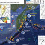
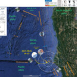
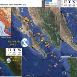
There was an earthquake yesterday in the Gulf of California nearby a series of earthquakes that happened in 2015 and earlier in 2013. The 2017 and 2013 earthquakes are happening along a fault that forms the Carmen Basin and the 2015 earthquakes are rupturing a fault that appears to be in the middle of the Farallon Basin. Here is my Earthquake Report for the 2013 earthquake (an early report, so it is rather basic). Here is my Earthquake Report for the 2015 earthquake sequence. This is an update to the initial 2015 report.
Below is my interpretive poster for this earthquake.
I plot the seismicity from the past month, with color representing depth and diameter representing magnitude (see legend). I include the USGS epicenters for earthquakes from 1917-2017 with magnitudes M ≥ 6.5.
I placed a moment tensor / focal mechanism legend on the poster. There is more material from the USGS web sites about moment tensors and focal mechanisms (the beach ball symbols). Both moment tensors and focal mechanisms are solutions to seismologic data that reveal two possible interpretations for fault orientation and sense of motion. One must use other information, like the regional tectonics, to interpret which of the two possibilities is more likely. I suspect that the fault that ruptured is eastward vergent (dipping to the west), so the west dipping nodal plane is probably the primary fault plane. However, this region of Kamchatka has numerous upper plate thrust and reverse faults (so the primary fault plane could be the other one, dipping to the east).
I also include the shaking intensity contours on the map. These use the Modified Mercalli Intensity Scale (MMI; see the legend on the map). This is based upon a computer model estimate of ground motions, different from the “Did You Feel It?” estimate of ground motions that is actually based on real observations. The MMI is a qualitative measure of shaking intensity. More on the MMI scale can be found here and here. This is based upon a computer model estimate of ground motions, different from the “Did You Feel It?” estimate of ground motions that is actually based on real observations.
I include some inset figures in the poster.
In the upper left corner I include a map that shows the tectonic setting of this region, with the geological units colored relative to their age and type (marine or continental).This is from a paper that discusses the interaction between spreading ridges and subduction trenches (Fletcher et al., 2007).
In the upper right corner I include a larger saled version of this map with the same seismicity plotted, but without the MMI contours. One can see the shape of the seafloor and how this is formed due to plate tectonics. Note the spreading ridge in the lower right corner and the parallel ridges formed as the plates extend from the ridge. The magnitude scale is slightly different than the main map.
In the lower left corner I include a map from the 2015 earthquake series. I include this because I labeled the Basins formed by the enechelon steps in this plate boundary. In my 2015 report, I provide more maps that include the names of some of these fracture zones (the transform plate boundary strike-slip faults).
Here is a great diagram showing the major faults in the region. I include their figure caption below.
(A) Simplified map of the Gulf of California region and Baja California peninsula showing the present plate boundary and some major tectonic features related to the plate-tectonic history since 12 Ma. The Gulf extensional province in gray is bounded by the Main Gulf Escarpment (bold dashed lines), which runs through the Loreto area and is shown in Figure 3. The Salton trough in southern California is merely the northern part of the Gulf extensional province. (B) Map of part of the southern Gulf of California and Baja California peninsula showing bathymetry (in meters), the transform–spreading-ridge plate boundary, and the location of subsequent figures with maps. The bathymetry is after a map in Ness and Lyle (1991) and the transform–spreading-ridge plate boundary is from Lonsdale (1989). The lines with double arrows are the three proposed rift segments modified here after Axen (1995); MS—Mulege´ segment, LS—Loreto segment, TS—Timbabichi
segment.
This map shows the magnetic anomalies and the geologic map for the land and the youngest oceanic crust.
(A) Tectonic map of the southern Baja California microplate (BCM) and Gulf of California extensional province (GEP). The Magdalena fan is deposited on oceanic crust of the Farallon-derived Magdalena microplate located west of Baja California. Deep Sea Drilling Project Site 471 is shown as black dot on the Magdalena fan. Abbreviations: BCT—Baja California trench, BM—Bahia Magdalena, LC—Los Cabos block, T—Trinidad block, LP—La Paz, PV—Puerto Vallarta, SMSLF—Santa Margarita–San Lazaro fault, TAF—Tosco-Abreojos fault, TS—Todos Santos, V—Vizcaino peninsula. Geology is simplifi ed from Muehlberger (1996). Interpretation of marine magnetic anomalies, with numbers denoting the chron of positively magnetized stripes, is from Severinghaus and Atwater (1989) and Lonsdale (1991).
This map shows a more broad view of the magnetic anomalies through time.
Map-view time slices showing the widely accepted model for the two-phase kinematic evolution of plate margin shearing around the Baja California microplate. (A) Configuration of active ridge segments (pink) west of Baja California just before they became largely abandoned ca. 12.3 Ma. (B) It is thought that plate motion from 12.3 to 6 Ma was kinematically partitioned into dextral strike slip (325 km) on faults west of Baja California and orthogonal rifting in the Gulf of California (90 km). This is known as the protogulf phase of rifting. (C) From 6 to 0 Ma faults west of Baja California are thought to have died and all plate motion was localized in the Gulf of California, which accommodated ~345 km of integrated transtensional shearing. Despite its wide acceptance, our data preclude this kinematic model. In all frames, the modern coastline is blue. Continental crust that accommodated post–12.3 Ma shearing is dark brown. Unfaulted microplates of continental crust are light tan. Farallon-derived microplates are light green. Middle Miocene trench-filling deposits like the Magdalena fan are colored dark green. Deep Sea Drilling Project Site 471 is the black dot on the southern Magdalena microplate. Yellow line (296 km) in the northern Gulf of California connects correlated terranes of Oskin and Stock (2003). Maps have Universal Transverse Mercator zone 12 projection with mainland Mexico fixed in present position.
Here is the Earthquake Report Poster from the 2015 sequence.
This is a nice simple figure, from the University of Sydney here, showing the terminology of strike slip faulting. It may help with the following figures.
Here is a fault block diagram showing how strike-slip step overs can create localized compression (positive flower) or extension (negative flower). More on strike-slip tectonics (and the source of this image) here.
Here is another great figure showing how sedimentary basins can be developed as a result of step overs in strike slip fault systems (source: Becky Dorsey, University of Oregon, Dept. of Geological Sciences).
I also put together an animation of seismicity from 1065 – 2015. First, here is a map that shows the spatial extent of this animation.
Here is the animation link (2 MB mp4 file) if you cannot view the embedded video below. Note how the animation begins in 1965, but has the recent seismicity plotted for reference.
There have been two large magnitude earthquakes in this region over the past 50 years.
This is an animation from Tanya Atwater. Click on this link to take you to yt (if the embedded video below does not work).
Here is an animation from IRIS. This link takes you to yt (if you cannot view the embedded version below). Here is a link to download the 21 MB mp4 vile file.
This is a link to a tectonic summary map from the USGS. Click on the map below to download the 20 MB pdf file.
References:
Fletcher, J.M., Grove, M., Kimbrough, D., Lovera, O., and Gehrels, G.E., 2007. Ridge-trench interactions and the Neogene tectonic evolution of the Magdalena shelf and southern Gulf of California: Insights from detrital zircon U-Pb ages from the Magdalena fan and adjacent areas in GSA Bulletin, v. 119, no. 11/12, p. 1313-1336.
Umhoefer, P.J., Mayer, L., and Dorse, R.J., 2002. Evolution of the margin of the Gulf of California near Loreto, Baja California Peninsula, Mexico in GSA Bulletin, v. 114, no. 7, p. 849-868.
This earthquake happened last night as I was preparing course materials for this morning. Initially it was a magnitude 6.9, but later modified to be M 6.9.
This earthquake happened in an interesting region of the world where there is a junction between two plate boundaries, the Kamchatka subduction zone with the Aleutian subduction zone / Bering-Kresla Shear Zone. The Kamchatka Trench (KT) is formed by the subduction (a convergent plate boundary) beneath the Okhtosk plate (part of North America). The Aleutian Trench (AT) and Bering-Kresla Shear Zone (BKSZ) are formed by the oblique subduction of the Pacific plate beneath the Pacific plate. There is a deflection in the Kamchatka subduction zone north of the BKSZ, where the subduction trench is offset to the west. Some papers suggest the subduction zone to the north is a fossil (inactive) plate boundary fault system. There are also several strike-slip faults subparallel to the BKSZ to the north of the BKSZ. These are shown in two of the inset maps below.
Below is my interpretive poster for this earthquake.
I plot the seismicity from the past month, with color representing depth and diameter representing magnitude (see legend). I include the USGS epicenters for earthquakes from 1917-2017 with magnitudes M ≥ 7.0 (the search window is limited to the region west of the Amlia fracture zone).
I also include moment tensors for earthquakes associated with the Kamchatka-Kuril subduction zone. There are some interesting earthquakes plotted here:
The pair of earthquakes 2008.07.05 M 7.7 and 2013.05.24 M 8.3 are very deep earthquakes (the M 8.3 is one of the largest and deepest earthquake ever recorded by modern seismometers) and may be due to bending of the downgoing slab. Here is my report for the M 8.3 (it was an early report of mine).
The pair of earthquakes 2006.11.15 M 833 and 2007.01.13 M 8.1 are directly related to each other. Lay et al. (2009) discussed this earthquake sequence and how the 2006 subduction zone earthquake led to the 2007 outer-rise earthquake in the Pacific plate. Dr. Erica Emry studied this earthquake pair for her Ph.D. research. I also wrote a little about these earthquakes in my earthquake report here.
The largest earthquake plotted for this region is the 1952 M 9.0 earthquake (the large epicenter between teh 1993 and 1997 earthquakes. This earthquake is the 5th largest earthquake recorded by modern seismometers. However, there is no USGS moment tensor (I couldn’t find a focal mechanism either). This earthquake generated a tsunami that traveled across the Pacific.
I placed a moment tensor / focal mechanism legend on the poster. There is more material from the USGS web sites about moment tensors and focal mechanisms (the beach ball symbols). Both moment tensors and focal mechanisms are solutions to seismologic data that reveal two possible interpretations for fault orientation and sense of motion. One must use other information, like the regional tectonics, to interpret which of the two possibilities is more likely. I suspect that the fault that ruptured is eastward vergent (dipping to the west), so the west dipping nodal plane is probably the primary fault plane. However, this region of Kamchatka has numerous upper plate thrust and reverse faults (so the primary fault plane could be the other one, dipping to the east).
I also include the shaking intensity contours on the map. These use the Modified Mercalli Intensity Scale (MMI; see the legend on the map). This is based upon a computer model estimate of ground motions, different from the “Did You Feel It?” estimate of ground motions that is actually based on real observations. The MMI is a qualitative measure of shaking intensity. More on the MMI scale can be found here and here. This is based upon a computer model estimate of ground motions, different from the “Did You Feel It?” estimate of ground motions that is actually based on real observations.
I include the slab contours plotted (Hayes et al., 2012), which are contours that represent the depth to the subduction zone fault. These are mostly based upon seismicity. The depths of the earthquakes have considerable error and do not all occur along the subduction zone faults, so these slab contours are simply the best estimate for the location of the fault. The hypocentral depth of the M 5.5 plots this close to the location of the fault as mapped by Hayes et al. (2012).
I include some inset figures in the poster.
In the upper left corner I include a map that shows the tectonic setting of this region, with the major plate boundary faults and volcanic arc designated by triangles (Bindeman et al., 2002). I placed an orange circle in the general location of the M 6.6 earthquake (sized relative to the magnitude range in the main map). Note the reverse fault mapped to the northeast of the epicenter. This fault dips to the southeast, supporting the east dipping solution for the M 6.6 moment tensor. I post this figure and their figure caption below.
To the right of this figure, I include a figure from Portnyagin and Manea (2008 ) that shows a low angle oblique view of the downgoing Pacific plate slab. I post this figure and their figure caption below.
In the lower left corner I include a map from the USGS Open File report (Rhea et al., 2010) that explains the historic seismicity for this region. I also plot the epicenter (orange dot).
In the upper right corner I include a map that shows more details about the faulting in the region. I place the epicenter for the M 6.6 as an orange circle. The location of the cross section I-I’ (plotted in the lower right corner) is designated by a dashed purple line.
Here is the tectonic map from Bindeman et al., 2002. The original figure caption is below in blockquote.
Tectonic setting of the Sredinny and Ganal Massifs in Kamchatka. Kamchatka/Aleutian junction is modified after Gaedicke et al. (2000). Onland geology is after Bogdanov and Khain (2000). 1, Active volcanoes (a) and Holocene monogenic vents (b). 2, Trench (a) and pull-apart basin in the Aleutian transform zone (b). 3, Thrust (a) and normal (b) faults. 4, Strike-slip faults. 5–6, Sredinny Massif. 5, Amphibolite-grade felsic paragneisses of the Kolpakovskaya series. 6, Allochthonous metasedimentary and metavolcanic rocks of the Malkinskaya series. 7, The Kvakhona arc. 8, Amphibolites and gabbro (solid circle) of the Ganal Massif. Lower inset shows the global position of Kamchatka. Upper inset shows main Cretaceous-Eocene tectonic units (Bogdanov and Khain 2000): Western Kamchatka (WK) composite unit including the Sredinny Massif, the Kvakhona arc, and the thick pile of Upper Cretaceous marine clastic rocks; Eastern Kamchatka (EK) arc, and Eastern Peninsulas terranes (EPT). Eastern Kamchatka is also known as the Olyutorka-Kamchatka arc (Nokleberg et al. 1998) or the Achaivayam-Valaginskaya arc (Konstantinovskaya 2000), while Eastern Peninsulas terranes are also called Kronotskaya arc (Levashova et al. 2000).
This map shows the configuration of the subducting slab. The original figure caption is below in blockquote.
Kamchatka subduction zone. A: Major geologic structures at the Kamchatka–Aleutian Arc junction. Thin dashed lines show isodepths to subducting Pacific plate (Gorbatov et al., 1997). Inset illustrates major volcanic zones in Kamchatka: EVB—Eastern Volcanic Belt; CKD—Central
Kamchatka Depression (rift-like tectonic structure, which accommodates the northern end of EVB); SR—Sredinny Range. Distribution of Quaternary volcanic rocks in EVB and SR is shown in orange and green, respectively. Small dots are active vol canoes. Large circles denote CKD volcanoes: T—Tolbachik; K l — K l y u c h e v s k o y ; Z—Zarechny; Kh—Kharchinsky; Sh—Shiveluch; Shs—Shisheisky Complex; N—Nachikinsky. Location of profiles shown in Figures 2 and 3 is indicated. B: Three dimensional visualization of the Kamchatka subduction zone from the north. Surface relief is shown as semi-transparent layer. Labeled dashed lines and color (blue to red) gradation of subducting plate denote depths to the plate from the earth surface (in km). Bold arrow shows direction of Pacific Plate movement.
Here is the more detailed tectonic map from Konstantinovskaia et al. (2001).
This is the cross section associated with the above map.
Bindeman, I.N., Vinogradov, V.I., Valley, J.W., Wooden, J.L., and Natal’in, B.A., 2002. Archean Protolith and Accretion of Crust in Kamchatka: SHRIMP Dating of Zircons from Sredinny and Ganal Massifs in The Journal of Geology, v. 110, p. 271-289.
Konstantinovskaia, E.A., 2001. Arc-continent collision and subduction reversal in the Cenozoic evolution of the Northwest Pacific: and example from Kamchatka (NE Russia) in Tectonophysics, v. 333, p. 75-94.
Koulakov, I.Y., Dobretsov, N.L., Bushenkova, N.A., and Yakovlev, A.V., 2011. Slab shape in subduction zones beneath the Kurile–Kamchatka and Aleutian arcs based on regional tomography results in Russian Geology and Geophysics, v. 52, p. 650-667.
Krutikov, L., et al., 2008. Active Tectonics and Seismic Potential of Alaska, Geophysical Monograph Series 179, doi:10.1029/179GM07
In March of 1964, plate tectonics was still a hotly debated topic at scientific meetings worldwide. Some people still do not accept this theory (some Russian geologists favor alternative hypotheses; Shevchenko et al., 2006). At the time, there was some debate about whether the M 9.2 earthquake (the 2nd largest earthquake recorded with modern seismometers) was from a strike-slip or from a revers/thrust earthquake. Plafker and his colleagues found the evidence to put that debate to rest (see USGS video below).
I have prepared a new map showing the 1964 earthquake in context to the plate boundary using the same methods I have been using for my other earthquake reports. I also found a focal mechanism for this M 9.2 earthquake and included this on the map (Stauder and Bollinger, 1966).
Below is my interpretive poster for this earthquake.
I plot the seismicity from the past month, with color representing depth and diameter representing magnitude (see legend). I include a focal mechanism for the M 9.2 earthquake determined by Stauder and Bollinger (1966). I include the USGS epicenters for earthquakes with magnitudes M ≥ 7.0.
I placed a moment tensor / focal mechanism legend on the poster. There is more material from the USGS web sites about moment tensors and focal mechanisms (the beach ball symbols). Both moment tensors and focal mechanisms are solutions to seismologic data that reveal two possible interpretations for fault orientation and sense of motion. One must use other information, like the regional tectonics, to interpret which of the two possibilities is more likely.
I also include the shaking intensity contours on the map. These use the Modified Mercalli Intensity Scale (MMI; see the legend on the map). This is based upon a computer model estimate of ground motions, different from the “Did You Feel It?” estimate of ground motions that is actually based on real observations. The MMI is a qualitative measure of shaking intensity. More on the MMI scale can be found here and here. This is based upon a computer model estimate of ground motions, different from the “Did You Feel It?” estimate of ground motions that is actually based on real observations.
I include the slab contours plotted (Hayes et al., 2012), which are contours that represent the depth to the subduction zone fault. These are mostly based upon seismicity. The depths of the earthquakes have considerable error and do not all occur along the subduction zone faults, so these slab contours are simply the best estimate for the location of the fault. The hypocentral depth of the M 5.5 plots this close to the location of the fault as mapped by Hayes et al. (2012).
I include some inset figures in the poster.
In the upper left corner I include two maps from the USGS, both using the MMI scale of shaking intensity mentioned above. The map on the left is the USGS Shakemap. This is a map that shows an estimate of how strongly the ground would shake during this earthquake. This is based upon a numerical model using Ground Motion Prediction Equations (GMPE), which are empirical relations between fault types, earthquake magnitude, distance from the fault, and shaking intensity. The map on the right is based upon peoples’ direct observations. Below each map are plots that show how these models demonstrate that the MMI attenuates (diminishes) with distance. The lines are the empirical relations. The dots are the data points.
To the right of those maps and figures is a map produced by Dr. Peter Haeussler from the USGS Alaska Science Center (pheuslr at usgs.gov) that shows the historic earthquakes along the Aleutian-Alaska subduction zone.
In the lower right corner I include an inset map from the USGS Seismicity History poster for this region (Benz et al., 2011). There is one seismicity cross section with its locations plotted on the map. The USGS plot these hypocenters along this cross section E-E’ (in green).
In the upper right corner, I include a figure that shows the measurements of uplift and subsidence observed by Plafker and his colleagues following the earthquake (Plafker, 1969). This is shown in map view and as a cross section.
Below is an educational video from the USGS that presents material about subduction zones and the 1964 earthquake and tsunami in particular. Youtube Source IRIS mp4 file for downloading.
Credits:
Animation & graphics by Jenda Johnson, geologist
Directed by Robert F. Butler, University of Portland
U.S. Geological Survey consultants: Robert C. Witter, Alaska Science Center Peter J. Haeussler, Alaska Science Center
Narrated by Roger Groom, Mount Tabor Middle School
This is a map from Haeussler et al. (2014). The region in red shows the area that subsided and the area in blue shows the region that uplifted during the earthquake. These regions were originally measured in the field by George Plafker and published in several documents, including this USGS Professional Paper (Plafker, 1969).
Here is a cross section showing the differences of vertical deformation between the coseismic (during the earthquake) and interseismic (between earthquakes).
This figure, from Atwater et al. (2005) shows the earthquake deformation cycle and includes the aspect that the uplift deformation of the seafloor can cause a tsunami.
Here is a figure recently published in the 5th International Conference of IGCP 588 by the Division of Geological and Geophysical Surveys, Dept. of Natural Resources, State of Alaska (State of Alaska, 2015). This is derived from a figure published originally by Plafker (1969). There is a cross section included that shows how the slip was distributed along upper plate faults (e.g. the Patton Bay and Middleton Island faults).
Here is a graphic showing the sediment-stratigraphic evidence of earthquakes in Cascadia, but the analogy works for Alaska also. Atwater et al., 2005. There are 3 panels on the left, showing times of (1) prior to earthquake, (2) several years following the earthquake, and (3) centuries after the earthquake. Before the earthquake, the ground is sufficiently above sea level that trees can grow without fear of being inundated with salt water. During the earthquake, the ground subsides (lowers) so that the area is now inundated during high tides. The salt water kills the trees and other plants. Tidal sediment (like mud) starts to be deposited above the pre-earthquake ground surface. This sediment has organisms within it that reflect the tidal environment. Eventually, the sediment builds up and the crust deforms interseismically until the ground surface is again above sea level. Now plants that can survive in this environment start growing again. There are stumps and tree snags that were rooted in the pre-earthquake soil that can be used to estimate the age of the earthquake using radiocarbon age determinations. The tree snags form “ghost forests.
This is a photo that I took along the Seward HWY 1, that runs east of Anchorage along the Turnagain Arm. I attended the 2014 Seismological Society of America Meeting that was located in Anchorage to commemorate the anniversary of the Good Friday Earthquake. This is a ghost forest of trees that perished as a result of coseismic subsidence during the earthquake. Copyright Jason R. Patton (2014). This region subsided coseismically during the 1964 earthquake. Here are some photos from the paleoseismology field trip. (Please contact me for a higher resolution version of this image: quakejay at gmail.com)
Here is the USGS shakemap for this earthquake. The USGS used a fault model, delineated as black rectangles, to model ground shaking at the surface. The color scale refers to the Modified Mercalli Intensity scale, shown at the bottom.
There is a great USGS Open File Report that summarizes the tectonics of Alaska and the Aleutian Islands (Benz et al., 2011). I include a section of their poster here. Below is the map legend.
Most recently, there was an earthquake along the Alaska Peninsula, a M 7.1 on 2016.01.24. Here is my earthquake report for this earthquake. Here is a map for the earthquakes of magnitude greater than or equal to M 7.0 between 1900 and today. This is the USGS query that I used to make this map. One may locate the USGS web pages for all the earthquakes on this map by following that link.
Here is an interesting map from Atwater et al., 2001. This figure shows how the estuarine setting in Portage, Alaska (along Turnagain Arm, southeast of Anchorage) had recovered its ground surface elevation in a short time following the earthquake. Within a decade, the region that had coseismically subsided was supporting a meadow with shrubs. By 1980, a spruce tree was growing here. This recovery was largely due to sedimentation, but an unreconciled amount of postseismic tectonic uplift contributed also. I include their figure caption as a blockquote.
(A and B) Tectonic setting of the 1964 Alaska earthquake. Subsidence from Plafker (1969). (C) Postearthquake deposits and their geologic setting in the early 1970s. (D–F) Area around Portage outlined in C, showing the landscape two years before the earthquake (D), two years after the earthquake (E), and nine years after the earthquake (F). In F, location of benchmark P 73 is from http://www.ngs.noaa.gov/cgi-bin/ds2.prl and the Seward (D-6) SE 7.5-minute quadrangle, provisional edition of 1984.
Here is an animation that shows earthquakes of magnitude > 6.5 for the period from 1900-2016. Above is a map showing the region and below is the animation. This is the URL for the USGS query that I used to make this animation in Google Earth.
Here is a link to the file for the embedded video below (5 MB mp4)
Here is an animation that shows the seismic waves propagating from the 1964 earthquake (West et al., 2014).
Here is a link to the file for the embedded video below (5 MB mp4)
Here is the tsunami forecast animation from the National Tsunami Warning Center. Below the animation, I include their caption as a blockquote. This includes information about the earthquake and the formation of the warning center.
Here is a link to the file for the embedded video below (22 MB 720 mp4)
At 5:36 pm on Friday, March 27, 1964 (28 March, 03:36Z UTC) the largest earthquake ever measured in North America, and the second-largest recorded anywhere, struck 40 miles west of Valdez, Alaska in Prince William Sound with a moment magnitude we now know to be 9.2. Almost an hour and a half later the Honolulu Magnetic and Seismic Observatory (later renamed the Pacific Tsunami Warning Center, or PTWC) was able to issue its first “tidal wave advisory” that noted that a tsunami was possible and that it could arrive in the Hawaiian Islands five hours later. Upon learning of a tsunami observation in Kodiak Island, Alaska, an hour and a half later the Honolulu Observatory issued a formal “tidal wave/seismic sea-wave warning” cautioning that damage was possible in Hawaii and throughout the Pacific Ocean but that it was not possible to predict the intensity of the tsunami. The earthquake did in fact generate a tsunami that killed 124 people (106 in Alaska, 13 in California, and 5 in Oregon) and caused about $2.3 billion (2016 dollars) in property loss all along the Pacific coast of North America from Alaska to southern California and in Hawaii. The greatest wave heights were in Alaska at over 67 m or 220 ft. and waves almost 10 m or 32 ft high struck British Columbia, Canada. In the “lower 48” waves as high as 4.5 m or 15 ft. struck Washington, as high as 3.7 m or 12 ft. struck Oregon, and as high as 4.8 m or over 15 ft. struck California. Waves of similar size struck Hawaii at nearly 5 m or over 16 ft. high. Waves over 1 m or 3 ft. high also struck Mexico, Chile, and even New Zealand.
As part of its response to this event the United States government created a second tsunami warning facility in 1967 at the Palmer Observatory, Alaska–now called the National Tsunami Warning Center (NTWC, http://ntwc.arh.noaa.gov/ )–to help mitigate future tsunami threats to Alaska, Canada, and the U.S. Mainland.
Today, more than 50 years since the Great Alaska Earthquake, PTWC and NTWC issue tsunami warnings in minutes, not hours, after a major earthquake occurs, and will also forecast how large any resulting tsunami will be as it is still crossing the ocean. PTWC can also create an animation of a historical tsunami with the same tool that it uses to determine tsunami hazards in real time for any tsunami today: the Real-Time Forecasting of Tsunamis (RIFT) forecast model. The RIFT model takes earthquake information as input and calculates how the waves move through the world’s oceans, predicting their speed, wavelength, and amplitude. This animation shows these values through the simulated motion of the waves and as they travel through the world’s oceans one can also see the distance between successive wave crests (wavelength) as well as their height (half-amplitude) indicated by their color. More importantly, the model also shows what happens when these tsunami waves strike land, the very information that PTWC needs to issue tsunami hazard guidance for impacted coastlines. From the beginning the animation shows all coastlines covered by colored points. These are initially a blue color like the undisturbed ocean to indicate normal sea level, but as the tsunami waves reach them they will change color to represent the height of the waves coming ashore, and often these values are higher than they were in the deeper waters offshore. The color scheme is based on PTWC’s warning criteria, with blue-to-green representing no hazard (less than 30 cm or ~1 ft.), yellow-to-orange indicating low hazard with a stay-off-the-beach recommendation (30 to 100 cm or ~1 to 3 ft.), light red-to-bright red indicating significant hazard requiring evacuation (1 to 3 m or ~3 to 10 ft.), and dark red indicating a severe hazard possibly requiring a second-tier evacuation (greater than 3 m or ~10 ft.).
Toward the end of this simulated 24 hours of activity the wave animation will transition to the “energy map” of a mathematical surface representing the maximum rise in sea-level on the open ocean caused by the tsunami, a pattern that indicates that the kinetic energy of the tsunami was not distributed evenly across the oceans but instead forms a highly directional “beam” such that the tsunami was far more severe in the middle of the “beam” of energy than on its sides. This pattern also generally correlates to the coastal impacts; note how those coastlines directly in the “beam” are hit by larger waves than those to either side of it.
Plafker, G., 1969. Tectonics of the March 27, 1964 Alaska earthquake: U.S. Geological Survey Professional Paper 543–I, 74 p., 2 sheets, scales 1:2,000,000 and 1:500,000, http://pubs.usgs.gov/pp/0543i/.
Shevchenko, V.I., Lukk, A.A., and Prilepin, M.T., 2006. The Sumatra Earthquake of December 26, 2004, as an Event Unrelated to the Plate-Tectonic Process in the Lithosphere in Physics of the Solid Earth, v. 42, no. 12, p. 1018–1037.
Stauder. W. and Bollinger, G.A., 1966. The Focal Mechanism of the Alaska Earthquake of March 28, 1964, and of Its Aftershock Sequence in JGR, v. 71, no. 22, p. 5283-5296.
The M 6.1 was a well behaved subduction zone earthquake associated with subduction of the Solomon Sea plate beneath the Solomon Islands, an island arc formed between opposing subduction zones. The M 6.0 earthquake and related earthquakes are more interesting. Baldwin et al. (2012) and Holm et al. (2016) both consider the North Solomon Trench (NST) to be inactive subduction zone, while the South Solomon Trench (SST) is an active subduction zone fault. There were 9 earthquakes larger than magnitude 2.5. The depths ranged between 4.2 and 53 km. There does not appear to be any direction that favors a deepening trend (i.e. getting deeper in the direction of the downgoing subduction zone fault). It is possible that these depths are not well constrained (the M 6.0 has a 4.2 km depth). These NNT earthquakes are either related to the NST, related to crustal faults, or reactivation of NST fault structures. Regardless, these are some interesting and mysterious earthquakes.
Below is my interpretive poster for this earthquake.
I plot the seismicity from the past year, with color representing depth and diameter representing magnitude (see legend).
I placed a moment tensor / focal mechanism legend on the poster. There is more material from the USGS web sites about moment tensors and focal mechanisms (the beach ball symbols). Both moment tensors and focal mechanisms are solutions to seismologic data that reveal two possible interpretations for fault orientation and sense of motion. One must use other information, like the regional tectonics, to interpret which of the two possibilities is more likely. The moment tensor shows northeast-southwest compression, perpendicular to the convergence at these plate boundaries.
I also include the shaking intensity contours on the map. These use the Modified Mercalli Intensity Scale (MMI; see the legend on the map). This is based upon a computer model estimate of ground motions, different from the “Did You Feel It?” estimate of ground motions that is actually based on real observations. The MMI is a qualitative measure of shaking intensity. More on the MMI scale can be found here and here. This is based upon a computer model estimate of ground motions, different from the “Did You Feel It?” estimate of ground motions that is actually based on real observations.
I include the slab contours plotted (Hayes et al., 2012), which are contours that represent the depth to the subduction zone fault. These are mostly based upon seismicity. The depths of the earthquakes have considerable error and do not all occur along the subduction zone faults, so these slab contours are simply the best estimate for the location of the fault.
I include some inset figures.
In the upper right corner is a map from Holm et al. (2016) that shows various key elements of the plate configuration in this region. Colors representing the age of the crust shows how the Woodlark Basin has an active spreading ridge system with ridges striking East-West. Large Igneous Provinces are shown here in dark gray. A relevant cross section is C-D, with the location highlighted in magenta on the map. The cross section shows how the North Solomon Trench is configured.
In the lower left corner is a generalized tectonic map of the region from Holm et al., 2016. This map shows the major plate boundary faults. Active subduction zones have shaded triangle fault symbols, while inactive subduction zones have un-shaded triangle fault line symbols.
In the upper left corner a figure from Oregon State University, which are based upon Hamilton (1979). “Tectonic microplates of the Melanesian region. Arrows show net plate motion relative to the Australian Plate.” This is from Johnson, 1976.
In the lower right corner is a figure from Baldwin et al. (2012). This figure shows a series of cross sections along this convergent plate boundary from the Solomon Islands in the east to Papua New Guinea in the west. Cross sections ‘A’ and ‘B’ are the most representative for the earthquakes today. I placed the general location of these cross sections on the main map as dashed orange lines. I present the map and this figure again below, with their original captions.
The M 6.1 is probably related to a series of earthquakes, including two M 7.9 megathrust events, further north along the San Crostobal Trench. Below are two earthquake interpretive posters for these earthquakes. This first poster is from my earthquake report on 2017.01.22.
Here is my interpretive poster from the 12/17 M 7.9 Bougainville Earthquake, possibly (probably) related to today’s M 7.9 earthquake. This is my Earthquake Report for the 12/17 earthquake.
In earlier earthquake reports, I discussed seismicity from 2000-2015 here. The seismicity on the west of this region appears aligned with north-south shortening along the New Britain trench, while seismicity on the east of this region appears aligned with more east-west shortening. Here is a map that I put together where I show these two tectonic domains with the seismicity from this time period (today’s earthquakes are not plotted on this map, but one may see where they might plot).
Background Figures
This figure shows an interpretation of the regional tectonics (Holm et al., 2016). I include the figure caption below as a blockquote.
Tectonic setting of Papua New Guinea and Solomon Islands. a) Regional plate boundaries and tectonic elements. Light grey shading illustrates bathymetry b 2000 m below sea level indicative of continental or arc crust, and oceanic plateaus; 1000 m depth contour is also shown. Adelbert Terrane (AT); Bismarck Sea fault (BSF); Bundi fault zone (BFZ); Feni Deep (FD); Finisterre Terrane (FT); Gazelle Peninsula (GP); Kia-Kaipito-Korigole fault zone (KKKF); Lagaip fault zone (LFZ); Mamberamo thrust belt (MTB); Manus Island (MI); New Britain (NB); New Ireland (NI); North Sepik arc (NSA); Ramu-Markham fault (RMF); Weitin Fault (WF);West Bismarck fault (WBF); Willaumez-Manus Rise (WMR).
This figure shows details of the regional tectonics (Holm et al., 2016). I include the figure caption below as a blockquote.
a) Present day tectonic features of the Papua New Guinea and Solomon Islands region as shown in plate reconstructions. Sea floor magnetic anomalies are shown for the Caroline plate (Gaina and Müller, 2007), Solomon Sea plate (Gaina and Müller, 2007) and Coral Sea (Weissel and Watts, 1979). Outline of the reconstructed Solomon Sea slab (SSP) and Vanuatu slab (VS)models are as indicated. b) Cross-sections related to the present day tectonic setting. Section locations are as indicated. Bismarck Sea fault (BSF); Feni Deep (FD); Louisiade Plateau
(LP); Manus Basin (MB); New Britain trench (NBT); North Bismarck microplate (NBP); North Solomon trench (NST); Ontong Java Plateau (OJP); Ramu-Markham fault (RMF); San Cristobal trench (SCT); Solomon Sea plate (SSP); South Bismarck microplate (SBP); Trobriand trough (TT); projected Vanuatu slab (VS); West Bismarck fault (WBF); West Torres Plateau (WTP); Woodlark Basin (WB).
This map shows plate velocities and euler poles for different blocks. Note the counterclockwise motion of the plate that underlies the Solomon Sea (Baldwin et al., 2012). I include the figure caption below as a blockquote.
Tectonic maps of the New Guinea region. (a) Seismicity, volcanoes, and plate motion vectors. Plate motion vectors relative to the Australian plate are surface velocity models based on GPS data, fault slip rates, and earthquake focal mechanisms (UNAVCO, http://jules.unavco.org/Voyager/Earth). Earthquake data are sourced from the International Seismological Center EHB Bulletin (http://www.isc.ac.uk); data represent events from January 1994 through January 2009 with constrained focal depths. Background image is generated from http://www.geomapapp.org. Abbreviations: AB, Arafura Basin; AT, Aure Trough; AyT, Ayu Trough; BA, Banda arc; BSSL, Bismarck Sea seismic lineation; BH, Bird’s Head; BT, Banda Trench; BTFZ, Bewani-Torricelli fault zone; DD, Dayman Dome; DEI, D’Entrecasteaux Islands; FP, Fly Platform; GOP, Gulf of Papua; HP, Huon peninsula; LA, Louisiade Archipelago; LFZ, Lowlands fault zone; MaT, Manus Trench; ML, Mt. Lamington; MT, Mt. Trafalgar; MuT, Mussau Trough; MV, Mt. Victory; MTB, Mamberamo thrust belt; MVF, Managalase Plateau volcanic field; NBT, New Britain Trench; NBA, New Britain arc; NF, Nubara fault; NGT, New Guinea Trench; OJP, Ontong Java Plateau; OSF, Owen Stanley fault zone; PFTB, Papuan fold-and-thrust belt; PP, Papuan peninsula; PRi, Pocklington Rise; PT, Pocklington Trough; RMF, Ramu-Markham fault; SST, South Solomons Trench; SA, Solomon arc; SFZ, Sorong fault zone; ST, Seram Trench; TFZ, Tarera-Aiduna fault zone; TJ, AUS-WDKPAC triple junction; TL, Tasman line; TT, Trobriand Trough;WD, Weber Deep;WB, Woodlark Basin;WFTB, Western (Irian) fold-and-thrust belt; WR,Woodlark Rift; WRi, Woodlark Rise; WTB, Weyland thrust; YFZ, Yapen fault zone.White box indicates the location shown in Figure 3. (b) Map of plates, microplates, and tectonic blocks and elements of the New Guinea region. Tectonic elements modified after Hill & Hall (2003). Abbreviations: ADB, Adelbert block; AOB, April ultramafics; AUS, Australian plate; BHB, Bird’s Head block; CM, Cyclops Mountains; CWB, Cendrawasih block; CAR, Caroline microplate; EMD, Ertsberg Mining District; FA, Finisterre arc; IOB, Irian ophiolite belt; KBB, Kubor & Bena blocks (including Bena Bena terrane); LFTB, Lengguru fold-and-thrust belt; MA, Mapenduma anticline; MB, Mamberamo Basin block; MO, Marum ophiolite belt; MHS, Manus hotspot; NBS, North Bismarck plate; NGH, New Guinea highlands block; NNG, Northern New Guinea block; OKT, Ok Tedi mining district; PAC, Pacific plate; PIC, Porgera intrusive complex; PSP, Philippine Sea plate; PUB, Papuan Ultramafic Belt ophiolite; SB, Sepik Basin block; SDB, Sunda block; SBS, South Bismarck plate; SIB, Solomon Islands block; WP, Wandamen peninsula; WDK, Woodlark microplate; YQ, Yeleme quarries.
This figure incorporates cross sections and map views of various parts of the regional tectonics (Baldwin et al., 2012). The New Britain region is in the map near the A and B sections. I include the figure caption below as a blockquote.
Oblique block diagram of New Guinea from the northeast with schematic cross sections showing the present-day plate tectonic setting. Digital elevation model was generated from http://www.geomapapp.org. Oceanic crust in tectonic cross sections is shown by thick black-and-white hatched lines, with arrows indicating active subduction; thick gray-and-white hatched lines indicate uncertain former subduction. Continental crust, transitional continental crust, and arc-related crust are shown without pattern. Representative geologic cross sections across parts of slices C and D are marked with transparent red ovals and within slices B and E are shown by dotted lines. (i ) Cross section of the Papuan peninsula and D’Entrecasteaux Islands modified from Little et al. (2011), showing the obducted ophiolite belt due to collision of the Australian (AUS) plate with an arc in the Paleogene, with later Pliocene extension and exhumation to form the D’Entrecasteaux Islands. (ii ) Cross section of the Papuan peninsula after Davies & Jaques (1984) shows the Papuan ophiolite thrust over metamorphic rocks of AUS margin affinity. (iii ) Across the Papuan mainland, the cross section after Crowhurst et al. (1996) shows the obducted Marum ophiolite and complex folding and thrusting due to collision of the Melanesian arc (the Adelbert, Finisterre, and Huon blocks) in the Late Miocene to recent. (iv) Across the Bird’s Head, the cross section after Bailly et al. (2009) illustrates deformation in the Lengguru fold-and-thrust belt as a result of Late Miocene–Early Pliocene northeast-southwest shortening, followed by Late Pliocene–Quaternary extension. Abbreviations as in Figure 2, in addition to NI, New Ireland; SI, Solomon Islands; SS, Solomon Sea; (U)HP, (ultra)high-pressure.
Background Videos
Here is an educational video (from IRIS) for this part of the western Pacific. There are many plate boundaries and these margins are very active. This is a link to the embedded video below (10.4 MB mp4)
I put together an animation that shows the seismicity for this region from 1900-2016 for earthquakes with magnitude of M ≥ 6.5. Here is the USGS query I used to search for these data used in this animation. I show the location of the Benz et al. (2011) cross section E-E’ as a yellow line on the main map.
In this animation, I include some figures from the interpretive poster above. I also include a tectonic map based upon Hamilton (1979). Music is from copyright free music online and is entitled “Sub Strut.” Above the video I present a map showing all the earthquakes presented in the video.
Geist, E.L., and Parsons, T., 2005, Triggering of tsunamigenic aftershocks from large strike-slip earthquakes: Analysis of the November 2000 New Ireland earthquake sequence: Geochemistry, Geophysics, Geosystems, v. 6, doi:10.1029/2005GC000935, 18 p. [Download PDF (6.5 MB)]
Holm, R.J., Rosenbaum, G, and Richards, S.W., 2016. Post 8 Ma reconstruction of Papua New Guinea and Solomon Islands: Microplate tectonics in a convergent plate boundary setting in Earth-Science Reviews, v. 156, pp. 66-81.
Johnson, R.W., 1976, Late Cainozoic volcanism and plate tectonics at the southern margin of the Bismarck Sea, Papua New Guinea, in Johnson, R.W., ed., 1976, Volcanism in Australia: Amsterdam, Elsevier, p. 101-116
Lay, T., and Kanamori, H., 1980, Earthquake doublets in the Solomon Islands: Physics of the Earth and Planetary Interiors, v. 21, p. 283-304.
Schwartz, S.Y., 1999, Noncharacteristic behavior and complex recurrence of large subduction zone earthquakes: Journal of Geophysical Research, v. 104, p. 23,111-123,125.
Schwartz, S.Y., Lay, T., and Ruff, L.J., 1989, Source process of the great 1971 Solomon Islands doublet: Physics of the Earth and Planetary Interiors, v. 56, p. 294-310.
Tregoning, P., McQueen, H., Lambeck, K., Jackson, R. Little, T., Saunders, S., and Rosa, R., 2000. Present-day crustal motion in Papua New Guinea, Earth Planets and Space, v. 52, pp. 727-730.
There were two interesting earthquakes near the northern tip of the Island of Sumatra whilst I was off on a field trip with some HSU geology students. So, I think it prudent to review these earthquakes now.
These earthquakes happened along the convergent plate boundary that is formed by the oblique subduction of the India-Australia plate beneath the Sunda plate (part of Eurasia). The India-Australia plate has numerous north-south striking fracture zones that are reactivated as normal faults when they reach the subduction trench (where the subducting plate flexes, causing bending and extension in the upper part of the plate). These fracture zones are initially strike-slip (or transform) faults.
In 2004 there was a Great megathrust earthquake (M =9.0)that triggered a catastrophic and deadly trans-oceanic tsunami. Three months later, in 2005, there was a triggered Great earthquake (M = 8.6), which also caused a tsunami, but a much smaller one for various reasons. The 2004 M 9.2 earthquake provided some ground breaking (sorry for the pun) advancements in our knowledge of the earth. One new observation is that this earthquake ruptured into the mantle, previously thought to behave in a ductile manner, so not capable of brittle failure during an earthquake. Earthquake reports for some of the earthquakes discussed on this page are listed at the bottom of the page.
In 2012, there was a series of Great earthquakes to the west of these 2004 & 2005 subduction zone earthquakes in a region that experienced increased strain following the 2004/2005 earthquakes. These two earthquakes initially appeared to have ocurred on one of these fracture zone faults. However, upon further investigations (including various analyses and aftershock analysis), these two earthquakes were actually along faults ~orthogonal to the fracture zones. They were also very very deep, also probably occurring in the mantle! But, the crust is really thick here (possibly the thickest oceanic crust in the world, associated with the ninetyeast ridge. The 90E ridge is thickened because the I-A plate floated over a hotspot, causing it to be thicker). The larger of the two had a magnitude of M = 8.6, which is currently the largest strike-slip earthquake ever recorded on modern seismometers. Later, on 2016.03.02, there was another strike-slip fault in the I-A plate. Assistant Professor Wei Shengi (Earth Observatory of Singapore) derived some slip models for this earthquake and chose a slip model based on an East-West fault, making it a right lateral strike-slip earthquake (EOS, 2016).
Here are the USGS websites for these two earthquakes.
There was an earthquake with a magnitude of M 6.0 that is just west of the tip of the megathrust fault, so is clearly in the India plate west of the subduction zone. This earthquake occurred on a strike-slip fault and is oriented similar to the 2012 and 2016 earthquakes. Like the 2016 earthquake, I am not sure which nodal plane is the fault plane and which is the auxiliary fault plane.
About 10 hours later, there was an M 5.5 earthquake that has a hypocentral depth of 41.2 km. This depth is fully consistent with the depth of the subduction zone megathrust fault here (Hayes et al., 2012). The moment tensor is consistent with a thrust fault and the fault plane is probably the northeast shallowly dipping nodal plane.
Below is my interpretive poster for this earthquake.
I plot the seismicity from the past month, with color representing depth and diameter representing magnitude (see legend). I include the USGS moment tensors from these earthquakes.
I placed a moment tensor / focal mechanism legend on the poster. There is more material from the USGS web sites about moment tensors and focal mechanisms (the beach ball symbols). Both moment tensors and focal mechanisms are solutions to seismologic data that reveal two possible interpretations for fault orientation and sense of motion. One must use other information, like the regional tectonics, to interpret which of the two possibilities is more likely. The moment tensor for the M 6.0 compares well with other Wharton Basin earthquakes from the past (e.g. 2012 & 2016). The triggered M 5.5 earthquake was instead possibly a subduction zone earthquake.
I also include the shaking intensity contours on the map. These use the Modified Mercalli Intensity Scale (MMI; see the legend on the map). This is based upon a computer model estimate of ground motions, different from the “Did You Feel It?” estimate of ground motions that is actually based on real observations. The MMI is a qualitative measure of shaking intensity. More on the MMI scale can be found here and here. This is based upon a computer model estimate of ground motions, different from the “Did You Feel It?” estimate of ground motions that is actually based on real observations.
I include the slab contours plotted (Hayes et al., 2012), which are contours that represent the depth to the subduction zone fault. These are mostly based upon seismicity. The depths of the earthquakes have considerable error and do not all occur along the subduction zone faults, so these slab contours are simply the best estimate for the location of the fault. The hypocentral depth of the M 5.5 plots this close to the location of the fault as mapped by Hayes et al. (2012).
I include some inset figures in the poster.
In the upper right corner I include a map showing the plate tectonics of the region as well as earthquake rupture regions for historic subduction zone earthquakes. Bathymetry and topography data come from the Smith and Sandwell (1997) Space Shuttle Radar Topography (SRTM) data set. The India-Australia plate subducts northeastward beneath the Sunda plate (part of Eurasia; sz–subduction zone). Orange vectors plot India plate movement relative to Sunda, and black vectors plot Australia relative to Sunda (global positioning system velocity based on Nuvel-1A; Bock et al., 2003; Subarya et al., 2006). Historic ruptures (Bilham, 2005; Malik et al., 2011) are plotted in grey, calendar years are in white. The 2004 and 2005 slip contours are shown orange and green, respectively (Chlieh et al., 2007, fig. 11 therein; Chlieh et al., 2008, figure 20 therein). Bengal and Nicobar fans cover structures of the India-Australia plate in the northern part of the map; are dashed black lines delimit their southern boundaries (Stow et al., 1990). The 2004 and 2005 earthquake focal mechanisms are plotted.
In the lower right corner is a Time Space plot of seismicity from this region for the period of 1973-2012 (Hayes et al., 2013). Great earthquakes are represented by yellow stars on the map time-space plot. The epicenters from the 2012 earthquakes are plotted on this map, so the figure caption is incorrect in their publication (can’t be perfect). Note how the rate of seismicity (prior to 2004 and 2010) at and north of the latitude of the 2007-09-12 M 8.4 subduction zone earthquake (4° S) is lower than south of this latitude. Of particular interest is that there is a slightly higher rate of seismicity between 4° and 8°. Could this inform us about whether or not there will be a Great earthquake in this region of the subduction zone?
In the upper left corner is a map that has the same earthquake patches as in the plate tectonic map. The base map is the Magnetic Anomaly data (Maus et al., 2009). These magnetic data is a compilation of data from ships, satellites, and airborne platforms. The first order patterns of dark and light gray represents the change in magnetic polarity through time. These show up on the map as horizontal/East-West bars in the oceanic crust west of Sumatra. These horizontal bars are also offset along North-South fracture zones (strike slip faults). Ninetyeast Ridge and the Investigator fracture zone are labeled. The Wharton Ridge is a spreading center that went inactive ~45 million years ago, which is part of the diffuse plate boundary between the India and Australia plates.
Below that map is a tectonic map of the Wharton Basin from Earth Observatory of Singapore (EOS, 2012). The Wharton Basin is the ocean basin east of the Ninetyeast Ridge west of the Sunda Megathrust. This map shows some earthquake rupture areas and the plate boundary faults (including the forearc sliver fault, the Sumatra fault), and North-South fracture zones in the Wharton Basin. The 2012 earthquakes and earthquake fault ruptures are shown in red stars and red dashed lines. Aftershocks are plotted as red oranges. Note how these help us define the faults that ruptured.
In the lower left corner are two maps that show seismicity from the 2012 earthquakes. On the left is a map showing the Satellite Gravity Anomaly. Variations in gravity anomaly data represent variations in earth material properties (things that change the spatial distribution of gravitational force). On the right is a map that shows the Magnetic Anomaly (like my map above). Epicenters and moment tensors for these earthquakes are plotted on both maps. The upper-right panel shows how the authors interpret how the faults slipped.
Sumatra-Wharton Basin Eartquakes
Here is an interpretive map that shows the early 21st century Great Earthquakes in the Sumatra-Wharton Basin region. More interpretive maps can be found here.
Some of the Poster Figures
This is the magnetic anomaly map.
This is the historic earthquake map.
This is the EOS 2012 earthquake map.
Tectonic setting of the April 11, 2012 earthquake. Seafloor fault information from Dyment et al. (2007) and Jacob et al. (2009), Satish et al. (2011), Deplus et al. (1998).
This is the main figure from Hayes et al. (2013) from the Seismicity of the Earth series. There is a map with the slab contours and seismicity both colored vs. depth. There are also some cross sections of seismicity plotted, with locations shown on the map.
This is the map and Time-Space plot (Hayes et al. (2013).
These are the gravity and magnetic anomaly maps (Duputel et al., 2012). I include the figure caption below as a blockquote.
The 2012 Sumatra great earthquake sequence.(a) Map of the 2012 Sumatra great earthquake region. The 11 April 2012 mainshock can be decomposed into two subevents separated by about 200 km (green mechanisms and circles labeled I and II). The W phase and Global CMT (GCMT solution available in July 2012; Ekstrom et al.,2012.) single-point-source solutions for the mainshock (inset green mechanisms), the W phase solutions for the 10 January foreshock (blue mechanism), for the Mw 8.2 aftershock (yellow mechanism) and for the 5.8 < Mw < 8.2 aftershocks (red mechanisms) are shown. Yellow circles indicate the earthquake epicenters and magnitudes from the National Earthquake Information Center (NEIC)catalog between 1 January 1973 and 10 April 2012. Red circles show the events since the Mw 8.6 11 April 2012 earthquake through May 2012. White arrows indicate the direction of motion of the Australian plate relative to the Indian plate at about 13 mm/yr (De Mets et al.,2010). The red triangles on the globe indicate the locations of broadband stations RER and BFO. b) W phase waveforms recorded at station RER (epicentral distance delta = 43, azimuth phi = 235) and BFO(delta = 84, phi = 317) during the 11 Mw 8.6 April 2012 Sumatra earthquake. In each figure, the black trace is the vertical broad-band displacement data and the red trace is the very-long- period displacement data filtered in the 200–1000 s pass band. The W phase, body wave arrivals (P,PP, S,SS) and the Rayleigh wavetrain (R) are indicated.
These are the gravity and magnetic anomaly maps (Meng et al., 2012). I include the figure caption below as a blockquote.
Spatiotemporal distribution of HF radiation imaged by the (left) European and (right) Japanese networks. Colored circles and squares indicate the positions of primary and secondary peak HF radiation (from movies S1 and S2, respectively). Their size is scaled by beamforming amplitude, and their color indicates timing relative to hypocentral time (color scale in center). The secondary peaks of the MUSIC pseudo-spectrum are those at least 50% as large as the main peak in the same frame. The brown shaded circles in the right figure are the HF radiation peaks from the Mw 8.2 aftershock observed from Japan. The colored contours in the Sumatra subduction zone (left) represent the slip model of the 2004 Mw 9.1 Sumatra earthquake (28). The figure background is colored by the satellite gravity anomaly (left) in milligalileos (mgals) (color scale on bottom left) and the magnetic anomaly (right) in nanoteslas (color scale on bottom right). Black dots are the epicenters of the first day of aftershocks from the U.S. National Earthquake Information Center catalog. The big and small white stars indicate the hypocenter of the mainshock and Mw 8.2 aftershock. The moment tensors of the Mw 8.6 mainshock, Mw 8.2 aftershock, and double CMT solutions of the mainshock are shown as colored pink, yellow, red, and blue beach balls. The red line in the top left inset shows the boundary between the India (IN) and Sundaland (SU) plates (29). The patterned pink area is the diffuse deformation zone between the India and Australia plate. The red rectangular zone indicates the study area. The top right inset shows the interpreted fault planes (gray dashed lines) and rupture directions (colored arrows).
Abercrombie, R.E., Antolik, M., Ekstrom, G., 2003. The June 2000 Mw 7.9 earthquakes south of Sumatra: Deformation in the India–Australia Plate. Journal of Geophysical Research 108, 16.
Bassin, C., Laske, G. and Masters, G., The Current Limits of Resolution for Surface Wave Tomography in North America, EOS Trans AGU, 81, F897, 2000.
Bock, Y., Prawirodirdjo, L., Genrich, J.F., Stevens, C.W., McCaffrey, R., Subarya, C., Puntodewo, S.S.O., Calais, E., 2003. Crustal motion in Indonesia from Global Positioning System measurements: Journal of Geophysical Research, v. 108, no. B8, 2367, doi: 10.1029/2001JB000324.
Bothara, J., Beetham, R.D., Brunston, D., Stannard, M., Brown, R., Hyland, C., Lewis, W., Miller, S., Sanders, R., Sulistio, Y., 2010. General observations of effects of the 30th September 2009 Padang earthquake, Indonesia. Bulletin of the New Zealand Society for Earthquake Engineering 43, 143-173.
Chlieh, M., Avouac, J.-P., Hjorleifsdottir, V., Song, T.-R.A., Ji, C., Sieh, K., Sladen, A., Hebert, H., Prawirodirdjo, L., Bock, Y., Galetzka, J., 2007. Coseismic Slip and Afterslip of the Great (Mw 9.15) Sumatra-Andaman Earthquake of 2004. Bulletin of the Seismological Society of America 97, S152-S173.
Chlieh, M., Avouac, J.P., Sieh, K., Natawidjaja, D.H., Galetzka, J., 2008. Heterogeneous coupling of the Sumatran megathrust constrained by geodetic and paleogeodetic measurements: Journal of Geophysical Research, v. 113, B05305, doi: 10.1029/2007JB004981.
DEPLUS, C. et al., 1998 – Direct evidence of active derormation in the eastern Indian oceanic plate, Geology.
DYMENT, J., CANDE, S.C. & SINGH, S., 2007 – Oceanic lithosphere subducting beneath the Sunda Trench: the Wharton Basin revisited. European Geosciences Union General Assembly, Vienna, 15-20/05.
Hayes, G.P., Bernardino, Melissa, Dannemann, Fransiska, Smoczyk, Gregory, Briggs, Richard, Benz, H.M., Furlong, K.P., and Villaseñor, Antonio, 2013. Seismicity of the Earth 1900–2012 Sumatra and vicinity: U.S. Geological Survey Open-File Report 2010–1083-L, scale 1:6,000,000, https://pubs.usgs.gov/of/2010/1083/l/.
JACOB, J., DYMENT, J., YATHEESH, V. & BHATTACHARYA, G.C., 2009 – Marine magnetic anomalies in the NE Indian Ocean: the Wharton and Central Indian basins revisited. European Geosciences Union General Assembly, Vienna, 19-24/04.
Ji, C., D.J. Wald, and D.V. Helmberger, Source description of the 1999 Hector Mine, California earthquake; Part I: Wavelet domain inversion theory and resolution analysis, Bull. Seism. Soc. Am., Vol 92, No. 4. pp. 1192-1207, 2002.
Ishii, M., Shearer, P.M., Houston, H., Vidale, J.E., 2005. Extent, duration and speed of the 2004 Sumatra-Andaman earthquake imaged by the Hi-Net array. Nature 435, 933.
Kanamori, H., Rivera, L., Lee, W.H.K., 2010. Historical seismograms for unravelling a mysterious earthquake: The 1907 Sumatra Earthquake. Geophysical Journal International 183, 358-374.
Konca, A.O., Avouac, J., Sladen, A., Meltzner, A.J., Sieh, K., Fang, P., Li, Z., Galetzka, J., Genrich, J., Chlieh, M., Natawidjaja, D.H., Bock, Y., Fielding, E.J., Ji, C., Helmberger, D., 2008. Partial Rupture of a Locked Patch of the Sumatra Megathrust During the 2007 Earthquake Sequence. Nature 456, 631-635.
Maus, S., et al., 2009. EMAG2: A 2–arc min resolution Earth Magnetic Anomaly Grid compiled from satellite, airborne, and marine magnetic measurements, Geochem. Geophys. Geosyst., 10, Q08005, doi:10.1029/2009GC002471.
Malik, J.N., Shishikura, M., Echigo, T., Ikeda, Y., Satake, K., Kayanne, H., Sawai, Y., Murty, C.V.R., Dikshit, D., 2011. Geologic evidence for two pre-2004 earthquakes during recent centuries near Port Blair, South Andaman Island, India: Geology, v. 39, p. 559-562.
Meltzner, A.J., Sieh, K., Chiang, H., Shen, C., Suwargadi, B.W., Natawidjaja, D.H., Philobosian, B., Briggs, R.W., Galetzka, J., 2010. Coral evidence for earthquake recurrence and an A.D. 1390–1455 cluster at the south end of the 2004 Aceh–Andaman rupture. Journal of Geophysical Research 115, 1-46.
Meng, L., Ampuero, J.-P., Stock, J., Duputel, Z., Luo, Y., and Tsai, V.C., 2012. Earthquake in a Maze: Compressional Rupture Branching During the 2012 Mw 8.6 Sumatra Earthquake in Science, v. 337, p. 724-726.
Natawidjaja, D.H., Sieh, K., Chlieh, M., Galetzka, J., Suwargadi, B., Cheng, H., Edwards, R.L., Avouac, J., Ward, S.N., 2006. Source parameters of the great Sumatran megathrust earthquakes of 1797 and 1833 inferred from coral microatolls. Journal of Geophysical Research 111, 37.
Newcomb, K.R., McCann, W.R., 1987. Seismic History and Seismotectonics of the Sunda Arc. Journal of Geophysical Research 92, 421-439.
Philibosian, B., Sieh, K., Natawidjaja, D.H., Chiang, H., Shen, C., Suwargadi, B., Hill, E.M., Edwards, R.L., 2012. An ancient shallow slip event on the Mentawai segment of the Sunda megathrust, Sumatra. Journal of Geophysical Research 117, 12.
Prawirodirdjo, P., McCaffrey,R., Chadwell, D., Bock, Y, and Subarya, C., 2010. Geodetic observations of an earthquake cycle at the Sumatra subduction zone: Role of interseismic strain segmentation, JOURNAL OF GEOPHYSICAL RESEARCH, v. 115, B03414, doi:10.1029/2008JB006139
Rivera, L., Sieh, K., Helmberger, D., Natawidjaja, D.H., 2002. A Comparative Study of the Sumatran Subduction-Zone Earthquakes of 1935 and 1984. BSSA 92, 1721-1736.
Shearer, P., and Burgmann, R., 2010. Lessons Learned from the 2004 Sumatra-Andaman Megathrust Rupture, Annu. Rev. Earth Planet. Sci. v. 38, pp. 103–31
SATISH C. S, CARTON H, CHAUHAN A.S., et al., 2011 – Extremely thin crust in the Indian Ocean possibly resulting from Plume-Ridge Interaction, Geophysical Journal International.
Sieh, K., Natawidjaja, D.H., Meltzner, A.J., Shen, C., Cheng, H., Li, K., Suwargadi, B.W., Galetzka, J., Philobosian, B., Edwards, R.L., 2008. Earthquake Supercycles Inferred from Sea-Level Changes Recorded in the Corals of West Sumatra. Science 322, 1674-1678.
Singh, S.C., Carton, H.L., Tapponnier, P, Hananto, N.D., Chauhan, A.P.S., Hartoyo, D., Bayly, M., Moeljopranoto, S., Bunting, T., Christie, P., Lubis, H., and Martin, J., 2008. Seismic evidence for broken oceanic crust in the 2004 Sumatra earthquake epicentral region, Nature Geoscience, v. 1, pp. 5.
Smith, W.H.F., Sandwell, D.T., 1997. Global seafloor topography from satellite altimetry and ship depth soundings: Science, v. 277, p. 1,957-1,962.
Sorensen, M.B., Atakan, K., Pulido, N., 2007. Simulated Strong Ground Motions for the Great M 9.3 Sumatra–Andaman Earthquake of 26 December 2004. BSSA 97, S139-S151.
Subarya, C., Chlieh, M., Prawirodirdjo, L., Avouac, J., Bock, Y., Sieh, K., Meltzner, A.J., Natawidjaja, D.H., McCaffrey, R., 2006. Plate-boundary deformation associated with the great Sumatra–Andaman earthquake: Nature, v. 440, p. 46-51.
Tolstoy, M., Bohnenstiehl, D.R., 2006. Hydroacoustic contributions to understanding the December 26th 2004 great Sumatra–Andaman Earthquake. Survey of Geophysics 27, 633-646.
Zhu, Lupei, and Donald V. Helmberger. “Advancement in source estimation techniques using broadband regional seismograms.” Bulletin of the Seismological Society of America 86.5 (1996): 1634-1641.
We just had an interesting earthquake in the region of the Mendocino triple junction. Recent earthquakes in this region show different fault plane solutions, owing to complexity of this area.
In 1983 there was an earthquake ~10 km to the west of today’s earthquake which had a right-lateral oblique compressional focal mechanism. In 2015, there was an earthquake ~15 km to the east of today’s earthquake that also had a right-lateral strike-slip moment tensor. If today’s earthquake was oblique, it would be left-lateral extensional. Today’s earthquake is quite interesting. I will need to think about it further.
Here are some USGS websites for earthquakes discussed below.
Below is my interpretive poster for this earthquake.
I plot the seismicity from the past month, with color representing depth and diameter representing magnitude (see legend).
I placed a moment tensor / focal mechanism legend on the poster. There is more material from the USGS web sites about moment tensors and focal mechanisms (the beach ball symbols). Both moment tensors and focal mechanisms are solutions to seismologic data that reveal two possible interpretations for fault orientation and sense of motion. One must use other information, like the regional tectonics, to interpret which of the two possibilities is more likely. The moment tensor shows northwest-southeast compression. This is very strange. I initially thought it was a compressional earthquake (slightly oblique), but now interpret this as an extensional earthquake. I am struggling to explain this.
I also include the shaking intensity contours on the map. These use the Modified Mercalli Intensity Scale (MMI; see the legend on the map). This is based upon a computer model estimate of ground motions, different from the “Did You Feel It?” estimate of ground motions that is actually based on real observations. The MMI is a qualitative measure of shaking intensity. More on the MMI scale can be found here and here. This is based upon a computer model estimate of ground motions, different from the “Did You Feel It?” estimate of ground motions that is actually based on real observations.
I include the slab contours plotted (Hayes et al., 2012), which are contours that represent the depth to the subduction zone fault. These are mostly based upon seismicity. The depths of the earthquakes have considerable error and do not all occur along the subduction zone faults, so these slab contours are simply the best estimate for the location of the fault.
I include some inset figures in the poster.
In the upper right corner is a map of the Cascadia subduction zone (CSZ) and regional tectonic plate boundary faults. This is modified from several sources (Chaytor et al., 2004; Nelson et al., 2004)
Below the CSZ map is an illustration modified from Plafker (1972). This figure shows how a subduction zone deforms between (interseismic) and during (coseismic) earthquakes. Today’s earthquake did not occur along the CSZ, so did not produce crustal deformation like this. However, it is useful to know this when studying the CSZ.
In the upper left corner is a figure from Rollins and Stein (2010). In their paper they discuss how static coulomb stress changes from earthquakes may impart (or remove) stress from adjacent crust/faults. I also present their figure where they present seismic observations for the 1983.08.24 M 5.5 earthquake (Rollins and Stein list M 6.3).
In the lower left corner is a figure from Dengler et al. (1995) that shows focal mechanisms from earthquakes in this region, along the Mendocino fault. Today’s earthquake is near the 1994 earthquake.
Here is a map from Rollins and Stein, showing their interpretations of different historic earthquakes in the region. This was published in response to the January 2010 Gorda plate earthquake. The faults are from Chaytor et al. (2004). The 1980, 1992, 1994, 2005, and 2010 earthquakes are plotted and labeled. I did not mention the 2010 earthquake, but it most likely was just like 1980 and 2005, a left-lateral strike-slip earthquake on a northeast striking fault.
Tectonic configuration of the Gorda deformation zone and locations and source models for 1976–2010 M ≥ 5.9 earthquakes. Letters designate chronological order of earthquakes (Table 1 and Appendix A). Plate motion vectors relative to the Pacific Plate (gray arrows in main diagram) are from Wilson [1989], with Cande and Kent’s [1995] timescale correction.
Here is a large scale map of the 1983 earthquake. The mainshock epicenter is a black star and epicenters are denoted as white circles. This earthquake is interpreted to be strike slip oblique (compression).
Source models for earthquakes A and B, 26 November 1976, Mw = 6.7, and 8 November 1980, Mw = 7.3; C, 24 August 1983, Mw = 6.1 (poorly constrained); D, 10 September 1984, Mw = 6.6 (no model made); E, 31 July 1987, Mw = 6.0, “WS2008” refers to Waldhauser and Schaff ’s [2008] double‐difference catalog; F, 13 July 1991, Mw = 6.8 (poorly constrained); G, 16 August 1991 (2226 UTC), Mw = 6.3 (no model made), open circles are NCSN locations for 16 August 1991 (2226 UTC) to 17 August 1991 (2216 UTC); H, 17 August 1991 (1929 UTC),Mw = 6.1; I, 17 August 1991 (2217 UTC), Mw = 7.1 (no model made); J, 25 April 1992, Mw = 6.9, open circles are from Waldhauser and Schaff ’s [2008] earthquake locations for 25 April 1992 (1806 UTC) to 26 April 1992 (0741 UTC); K and L, 26 April 1992 (0741 UTC), Mw = 6.5 and 26 April 1992 (1118 UTC), Mw = 6.6 (both poorly constrained), seismicity shallower than 15 km was excluded so that shallow aftershocks of (J) do not crowd figure; M, 1 September 1994, Mw = 7.0; N and O, 19 February 1995, Mw = 6.6, and 16 March 2000, Mw = 5.9; P, Q, and R, 15 June 2005, Mw = 7.2, 17 June 2005, Mw = 6.6 (poorly constrained), and 28 November 2008, Mw = 5.9 (poorly constrained); S and T, 10 January 2010, M = 6.5, and 4 February 2010, Mw = 5.9; Z, 18 April 1906, M = 7.8.
Here is a plot of focal mechanisms from the Dengler et al. (1995) paper in California Geology.
In this map below, I label a number of other significant earthquakes in this Mendocino triple junction region. Another historic right-lateral earthquake on the Mendocino fault system was in 1994. There was a series of earthquakes possibly along the easternmost section of the Mendocino fault system in late January 2015, here is my post about that earthquake series.
There are three types of earthquakes, strike-slip, compressional (reverse or thrust, depending upon the dip of the fault), and extensional (normal). Here is are some animations of these three types of earthquake faults. Many of the earthquakes people are familiar with in the Mendocino triple junction region are either compressional or strike slip. The following three animations are from IRIS.
Strike Slip:
Compressional:
Extensional:
Here is a primer that helps people learn how to interpret focal mechanisms and moment tensors. Moment tensors are calculated differently from focal mechanisms, but the interpretation of their graphical solution is similar. This is from the USGS.
For more on the graphical representation of moment tensors and focal mechnisms, check this IRIS video out:
This figure shows what a transform plate boundary fault is. Looking down from outer space, the crust on either side of the fault moves side-by-side. When one is standing on the ground, on one side of the fault, looking across the fault as it moves… If the crust on the other side of the fault moves to the right, the fault is a “right lateral” strike slip fault. The Mendocino and San Andreas faults are right-lateral (dextral) strike-slip faults.
Here is an IRIS animation showing a transform plate boundary fault as it relates to spreading ridges.
Chaytor, J.D., Goldfinger, C., Dziak, R.P., and Fox, C.G., 2004. Active deformation of the Gorda plate: Constraining deformation models with new geophysical data: Geology v. 32, p. 353-356.
Irwin, W.P., 1990. Quaternary deformation, in Wallace, R.E. (ed.), 1990, The San Andreas Fault system, California: U.S. Geological Survey Professional Paper 1515, online at: http://pubs.usgs.gov/pp/1990/1515/
McLaughlin, R.J., Sarna-Wojcicki, A.M., Wagner, D.L., Fleck, R.J., Langenheim, V.E., Jachens, R.C., Clahan, K., and Allen, J.R., 2012. Evolution of the Rodgers Creek–Maacama right-lateral fault system and associated basins east of the northward-migrating Mendocino Triple Junction, northern California in Geosphere, v. 8, no. 2., p. 342-373.
Nelson, A.R., Asquith, A.C., and Grant, W.C., 2004. Great Earthquakes and Tsunamis of the Past 2000 Years at the Salmon River Estuary, Central Oregon Coast, USA: Bulletin of the Seismological Society of America, Vol. 94, No. 4, pp. 1276–1292
Rollins, J.C. and Stein, R.S., 2010. Coulomb stress interactions among M ≥ 5.9 earthquakes in the Gorda deformation zone and on the Mendocino Fault Zone, Cascadia subduction zone, and northern San Andreas Fault: Journal of Geophysical Research, v. 115, B12306, doi:10.1029/2009JB007117, 2010.
Stoffer, P.W., 2006, Where’s the San Andreas Fault? A guidebook to tracing the fault on public lands in the San Francisco Bay region: U.S. Geological Survey General Interest Publication 16, 123 p., online at http://pubs.usgs.gov/gip/2006/16/
Wallace, Robert E., ed., 1990, The San Andreas fault system, California: U.S. Geological Survey Professional Paper 1515, 283 p. [http://pubs.usgs.gov/pp/1988/1434/].
We just had an earthquake with a USGS magnitude of M 6.5 along the subduction zone formed by the convergence of the Solomon Sea plate on the south and the South Bismarck plate on the north.
Here is the USGS website for this M 6.5 earthquake.
Below is my interpretive poster for this earthquake.
I plot the seismicity from the past month, with color representing depth and diameter representing magnitude (see legend). I also include seismicity from 1917-2017 for earthquakes with magnitudes M ≥ 7.0. I include the USGS moment tensor from this earthquake.
I placed a moment tensor / focal mechanism legend on the poster. There is more material from the USGS web sites about moment tensors and focal mechanisms (the beach ball symbols). Both moment tensors and focal mechanisms are solutions to seismologic data that reveal two possible interpretations for fault orientation and sense of motion. One must use other information, like the regional tectonics, to interpret which of the two possibilities is more likely. The moment tensor shows northeast-southwest compression, perpendicular to the convergence at this plate boundary.
I also include the shaking intensity contours on the map. These use the Modified Mercalli Intensity Scale (MMI; see the legend on the map). This is based upon a computer model estimate of ground motions, different from the “Did You Feel It?” estimate of ground motions that is actually based on real observations. The MMI is a qualitative measure of shaking intensity. More on the MMI scale can be found here and here. This is based upon a computer model estimate of ground motions, different from the “Did You Feel It?” estimate of ground motions that is actually based on real observations.
I include the slab contours plotted (Hayes et al., 2012), which are contours that represent the depth to the subduction zone fault. These are mostly based upon seismicity. The depths of the earthquakes have considerable error and do not all occur along the subduction zone faults, so these slab contours are simply the best estimate for the location of the fault. The hypocentral depth plots this close to the location of the fault as mapped by Hayes et al. (2012). This earthquake appears to be in the upper plate based upon the hypocentral depth of <30 km and the slab contour of 60 km at this location, though this is unclear.
I include some inset figures in the poster.
At the top of the poster are two figures from Oregon State University, which are based upon Hamilton (1979). “Tectonic microplates of the Melanesian region. Arrows show net plate motion relative to the Australian Plate.” To the right of the map is a cross section showing how the Solomon Sea plate is subducting beneath New Britain. This is from Johnson, 1976.
In the upper right corner are two figures from Holm and Richards (2013). Their paper discusses the back-arc spreading in the Bismarck Sea. They use hypocenter data to construct this 3-D model of the slab. On the right is a forecast of how the slab will be consumed along these subduction zones in the future.
In the lower right corner is a cross sectional view of the New Britain subduction zone for the past 10 million years (Holm and Richards, 2013). The approximate location of for this cross section is designated by an orange dashed line on the main map, with N and S labels.
In the upper left corner is a figure from Baldwin et al. (2012). This figure shows a series of cross sections along this convergent plate boundary from the Solomon Islands in the east to Papua New Guinea in the west. Cross section ‘C’ is the most representative for the earthquake today. I place the general location of the C-C’ section on the main map as an orange dashed line. I present the map and this figure again below, with their original captions.
In the lower left corner is the map from Baldwin et al. (2012) that goes along with the cross sections above.
This is a map showing the seismicity of this region since 2000 A.D.
Earlier, I discussed seismicity from 2000-2015 here. The seismicity on the west of this region appears aligned with north-south shortening along the New Britain trench, while seismicity on the east of this region appears aligned with more east-west shortening. Here is a map that I put together where I show these two tectonic domains with the seismicity from this time period (today’s earthquakes are not plotted on this map, but one may see where they might plot).
Here is the generalized tectonic map of the region from Holm et al., 2015. I include the figure caption below as a blockquote.
Tectonic setting and mineral deposits of eastern Papua New Guinea and Solomon Islands. The modern arc setting related to formation of the mineral deposits comprises, from west to east, the West Bismarck arc, the New Britain arc, the Tabar-Lihir-Tanga-Feni Chain and the Solomon arc, associated with north-dipping subduction/underthrusting at the Ramu-Markham fault zone, New Britain trench and San Cristobal trench respectively. Arrows denote plate motion direction of the Australian and Pacific plates. Filled triangles denote active subduction. Outlined triangles denote slow or extinct subduction. NBP: North Bismarck plate; SBP: South Bismarck plate; AT: Adelbert Terrane; FT: Finisterre Terrane; RMF: Ramu-Markham fault zone; NBT: New Britain trench.
Here is the slab interpretation for the New Britain region from Holm and Richards, 2013. I include the figure caption below as a blockquote.
3-D model of the Solomon slab comprising the subducted Solomon Sea plate, and associated crust of the Woodlark Basin and Australian plate subducted at the New Britain and San Cristobal trenches. Depth is in kilometres; the top surface of the slab is contoured at 20 km intervals from the Earth’s surface (black) to termination of slabrelated seismicity at approximately 550 km depth (light brown). Red line indicates the locations of the Ramu-Markham Fault (RMF)–New Britain trench (NBT)–San Cristobal trench (SCT); other major structures are removed for clarity; NB, New Britain; NI, New Ireland; SI, Solomon Islands; SS, Solomon Sea; TLTF, Tabar–Lihir–Tanga–Feni arc. See text for details.
Here are the forward models for the slab in the New Britain region from Holm and Richards, 2013. I include the figure caption below as a blockquote.
Forward tectonic reconstruction of progressive arc collision and accretion of New Britain to the Papua New Guinea margin. (a) Schematic forward reconstruction of New Britain relative to Papua New Guinea assuming continued northward motion of the Australian plate and clockwise rotation of the South Bismarck plate. (b) Cross-sections illustrate a conceptual interpretation of collision between New Britain and Papua New Guinea.
This map shows plate velocities and euler poles for different blocks. Note the counterclockwise motion of the plate that underlies the Solomon Sea (Baldwin et al., 2012). I include the figure caption below as a blockquote.
Tectonic maps of the New Guinea region. (a) Seismicity, volcanoes, and plate motion vectors. Plate motion vectors relative to the Australian plate are surface velocity models based on GPS data, fault slip rates, and earthquake focal mechanisms (UNAVCO, http://jules.unavco.org/Voyager/Earth). Earthquake data are sourced from the International Seismological Center EHB Bulletin (http://www.isc.ac.uk); data represent events from January 1994 through January 2009 with constrained focal depths. Background image is generated from http://www.geomapapp.org. Abbreviations: AB, Arafura Basin; AT, Aure Trough; AyT, Ayu Trough; BA, Banda arc; BSSL, Bismarck Sea seismic lineation; BH, Bird’s Head; BT, Banda Trench; BTFZ, Bewani-Torricelli fault zone; DD, Dayman Dome; DEI, D’Entrecasteaux Islands; FP, Fly Platform; GOP, Gulf of Papua; HP, Huon peninsula; LA, Louisiade Archipelago; LFZ, Lowlands fault zone; MaT, Manus Trench; ML, Mt. Lamington; MT, Mt. Trafalgar; MuT, Mussau Trough; MV, Mt. Victory; MTB, Mamberamo thrust belt; MVF, Managalase Plateau volcanic field; NBT, New Britain Trench; NBA, New Britain arc; NF, Nubara fault; NGT, New Guinea Trench; OJP, Ontong Java Plateau; OSF, Owen Stanley fault zone; PFTB, Papuan fold-and-thrust belt; PP, Papuan peninsula; PRi, Pocklington Rise; PT, Pocklington Trough; RMF, Ramu-Markham fault; SST, South Solomons Trench; SA, Solomon arc; SFZ, Sorong fault zone; ST, Seram Trench; TFZ, Tarera-Aiduna fault zone; TJ, AUS-WDKPAC triple junction; TL, Tasman line; TT, Trobriand Trough;WD, Weber Deep;WB, Woodlark Basin;WFTB, Western (Irian) fold-and-thrust belt; WR,Woodlark Rift; WRi, Woodlark Rise; WTB, Weyland thrust; YFZ, Yapen fault zone.White box indicates the location shown in Figure 3. (b) Map of plates, microplates, and tectonic blocks and elements of the New Guinea region. Tectonic elements modified after Hill & Hall (2003). Abbreviations: ADB, Adelbert block; AOB, April ultramafics; AUS, Australian plate; BHB, Bird’s Head block; CM, Cyclops Mountains; CWB, Cendrawasih block; CAR, Caroline microplate; EMD, Ertsberg Mining District; FA, Finisterre arc; IOB, Irian ophiolite belt; KBB, Kubor & Bena blocks (including Bena Bena terrane); LFTB, Lengguru fold-and-thrust belt; MA, Mapenduma anticline; MB, Mamberamo Basin block; MO, Marum ophiolite belt; MHS, Manus hotspot; NBS, North Bismarck plate; NGH, New Guinea highlands block; NNG, Northern New Guinea block; OKT, Ok Tedi mining district; PAC, Pacific plate; PIC, Porgera intrusive complex; PSP, Philippine Sea plate; PUB, Papuan Ultramafic Belt ophiolite; SB, Sepik Basin block; SDB, Sunda block; SBS, South Bismarck plate; SIB, Solomon Islands block; WP, Wandamen peninsula; WDK, Woodlark microplate; YQ, Yeleme quarries.
This figure incorporates cross sections and map views of various parts of the regional tectonics (Baldwin et al., 2012). The New Britain region is in the map near the A and B sections. I include the figure caption below as a blockquote.
Oblique block diagram of New Guinea from the northeast with schematic cross sections showing the present-day plate tectonic setting. Digital elevation model was generated from http://www.geomapapp.org. Oceanic crust in tectonic cross sections is shown by thick black-and-white hatched lines, with arrows indicating active subduction; thick gray-and-white hatched lines indicate uncertain former subduction. Continental crust, transitional continental crust, and arc-related crust are shown without pattern. Representative geologic cross sections across parts of slices C and D are marked with transparent red ovals and within slices B and E are shown by dotted lines. (i ) Cross section of the Papuan peninsula and D’Entrecasteaux Islands modified from Little et al. (2011), showing the obducted ophiolite belt due to collision of the Australian (AUS) plate with an arc in the Paleogene, with later Pliocene extension and exhumation to form the D’Entrecasteaux Islands. (ii ) Cross section of the Papuan peninsula after Davies & Jaques (1984) shows the Papuan ophiolite thrust over metamorphic rocks of AUS margin affinity. (iii ) Across the Papuan mainland, the cross section after Crowhurst et al. (1996) shows the obducted Marum ophiolite and complex folding and thrusting due to collision of the Melanesian arc (the Adelbert, Finisterre, and Huon blocks) in the Late Miocene to recent. (iv) Across the Bird’s Head, the cross section after Bailly et al. (2009) illustrates deformation in the Lengguru fold-and-thrust belt as a result of Late Miocene–Early Pliocene northeast-southwest shortening, followed by Late Pliocene–Quaternary extension. Abbreviations as in Figure 2, in addition to NI, New Ireland; SI, Solomon Islands; SS, Solomon Sea; (U)HP, (ultra)high-pressure.
New Britain | Solomon | Bougainville | New Hebrides | Tonga | Kermadec
Johnson, R.W., 1976, Late Cainozoic volcanism and plate tectonics at the southern margin of the Bismarck Sea, Papua New Guinea, in Johnson, R.W., ed., 1976, Volcanism in Australia: Amsterdam, Elsevier, p. 101-116
Tregoning, P., McQueen, H., Lambeck, K., Jackson, R. Little, T., Saunders, S., and Rosa, R., 2000. Present-day crustal motion in Papua New Guinea, Earth Planets and Space, v. 52, pp. 727-730.
Earlier this week there was a moderate earthquake along a strike-slip fault that appears to adjoin the Banda/Timor/Java Arc with New Guinea. This strike-slip fault appears to cross oblique to the subduction zone that forms the Timor Trench to the south and the Seram Trench to the north. Various researchers portray the faulting in this region differently. Given earthquake moment tensor and focal mechanism from the USGS, this earthquake supports the interpretation that this fault system is left-lateral (synistral) strike-slip. A focal mechanism from an earthquake in 1938 (magnitude M 8.5) provides evidence that is a little more confusing. But, this region is a complicated region.
UPDATE: 2017.03.05 (23:00 local time): Interesting, I was reading my tweet after Lila Lisle noticed a mistake. I fixed that, but later realized that the possible fault in the downgoing plate is not the Sorog fault, but a fault that might intersect with the Sorong fault. I did not delete the tweet since this mistake is a topic of conversation and not really a key part of the story.
Here is the USGS earthquake website for this M 5.5 earthquake.
Here are the USGS websites for the major earthquakes in this region from the past century.
Below is my interpretive poster for this earthquake.
I plot the seismicity from the past month, with color representing depth and diameter representing magnitude (see legend). I also include seismicity from 1917-2017 for earthquakes with magnitudes M ≥ 7.0. I show the fault plane solutions for some of these earthquakes.
moment tensors for 2005, 2012, and 2017 (USGS)
focal mechanisms for 1987 (USGS) and 1938 (Okal and Reymond, 2003)
The fault plane solutions for the 1963, 1987, 2005, and 2012 earthquakes are all very similar to the 2017 M 5.5. However, these earthquakes are form two depth “populations.” The 1963 and 1987 earthquakes are at ~65 km depth, while the 2005, 2012, and 2017 are between 150-200 km. There are some earthquakes that are much shallower depth eastward along this possibly strike-slip fault. Near where this fault comes on land at the base of the Bird’s Head in New Guinea, there are some earthquakes from the past couple of decades that also have strike-slip fault–plane solutions. The earthquake depths along this Sorong fault (Hall, 2011) appear to show that the Sorong fault is active beneath the Sunda plate. The 1938 earthquake may be the result of some form of strain partitioned faulting(?). Alternatively, these earthquakes may be unrelated to the Sorong fault. There may be some internal structure in the Australia plate that is interacting with the subduction zones or other faults (some preexisting structure that is optimally oriented to reactivate with the .
I placed a moment tensor / focal mechanism legend on the poster. There is more material from the USGS web sites about moment tensors and focal mechanisms (the beach ball symbols). Both moment tensors and focal mechanisms are solutions to seismologic data that reveal two possible interpretations for fault orientation and sense of motion. One must use other information, like the regional tectonics, to interpret which of the two possibilities is more likely
I also include the shaking intensity contours on the map. These use the Modified Mercalli Intensity Scale (MMI; see the legend on the map). This is based upon a computer model estimate of ground motions, different from the “Did You Feel It?” estimate of ground motions that is actually based on real observations. The MMI is a qualitative measure of shaking intensity. More on the MMI scale can be found here and here. This is based upon a computer model estimate of ground motions, different from the “Did You Feel It?” estimate of ground motions that is actually based on real observations.
I include the slab contours plotted (Hayes et al., 2012), which are contours that represent the depth to the subduction zone fault. These are mostly based upon seismicity. The depths of the earthquakes have considerable error and do not all occur along the subduction zone faults, so these slab contours are simply the best estimate for the location of the fault. The hypocentral depth plots this close to the location of the fault as mapped by Hayes et al. (2012).
I include some inset figures in the poster.
In the upper left corner is a general tectonic map for this part of the world. I placed a green star in the location of this M 5.5 earthquake (Zahirovic et al., 2014).
In the upper right corner is a low-angle oblique view of the plate boundaries in the northern part of this region (Hall, 2011). The upper part of the diagram shows the opposing vergent subduction zones along that strike north-south along the Molucca Strait (Halmahera, Philippines). The lower panel shows the downgoing Australia plate along the Timor Trench and Seram Trench. Note the location of the Bird’s Head, the northwestern part of New Guinea. I have also labeled this region in the main map for comparison. The strike-slip fault at the northern boundary of New Guinea is the Sorong fault and this is labeled in this Hall (2011) figure.
Below the Hall (2011) figure is a figure from Baldwin et al. (2012) that shows the regional seismicity and faulting as they are related to different geologic types in New Guinea. I placed a green star in the location of this M 5.5 earthquake.
In the lower right corner is a part of the USGS Poster that reviews the seismicity of this region for the past century or so (Benz et a., 2011). The map shows seismicity with depth, along with some cross section locations. I place a green star at the location of this M 5.5 earthquake. I present three of the cross sections from this poster, A-A’, B-B’, and C-C.’ Of particular interest is the section B-B’ because this is placed near the M 5.5 earthquake. I have placed a green star that represents the hypocentral location on cross section B-B.’ The hypocentral depth suggests this M 5.5 earthquake is in the downgoing Australia plate slab.
In the lower left corner is a diagram showing the subducting Australia plate at the Java Trench (Yves Descatoire).
To the right of the Java Trench figure presents a detailed view of the faulting along the eastern Java and western Timor trenches (Hangesh and Whitney, 2016). They present evidence for oblique motion along the Timor trough. And present evidence for a backthrust on the northern side of Timor and the Indonesia islands east of Java.
Tectonic maps of the New Guinea region. (a) Seismicity, volcanoes, and plate motion vectors. Plate motion vectors relative to the Australian plate are surface velocity models based on GPS data, fault slip rates, and earthquake focal mechanisms (UNAVCO, http://jules.unavco.org/Voyager/Earth). Earthquake data are sourced from the International Seismological Center EHB Bulletin (http://www.isc.ac.uk); data represent events from January 1994 through January 2009 with constrained focal depths. Background image is generated from http://www.geomapapp.org. Abbreviations: AB, Arafura Basin; AT, Aure Trough; AyT, Ayu Trough; BA, Banda arc; BSSL, Bismarck Sea seismic lineation; BH, Bird’s Head; BT, Banda Trench; BTFZ, Bewani-Torricelli fault zone; DD, Dayman Dome; DEI, D’Entrecasteaux Islands; FP, Fly Platform; GOP, Gulf of Papua; HP, Huon peninsula; LA, Louisiade Archipelago; LFZ, Lowlands fault zone; MaT, Manus Trench; ML, Mt. Lamington; MT, Mt. Trafalgar; MuT, Mussau Trough; MV, Mt. Victory; MTB, Mamberamo thrust belt; MVF, Managalase Plateau volcanic field; NBT, New Britain Trench; NBA, New Britain arc; NF, Nubara fault; NGT, New Guinea Trench; OJP, Ontong Java Plateau; OSF, Owen Stanley fault zone; PFTB, Papuan fold-and-thrust belt; PP, Papuan peninsula; PRi, Pocklington Rise; PT, Pocklington Trough; RMF, Ramu-Markham fault; SST, South Solomons Trench; SA, Solomon arc; SFZ, Sorong fault zone; ST, Seram Trench; TFZ, Tarera-Aiduna fault zone; TJ, AUS-WDKPAC triple junction; TL, Tasman line; TT, Trobriand Trough;WD, Weber Deep;WB, Woodlark Basin;WFTB, Western (Irian) fold-and-thrust belt; WR,Woodlark Rift; WRi, Woodlark Rise; WTB, Weyland thrust; YFZ, Yapen fault zone.White box indicates the location shown in Figure 3. (b) Map of plates, microplates, and tectonic blocks and elements of the New Guinea region. Tectonic elements modified after Hill & Hall (2003). Abbreviations: ADB, Adelbert block; AOB, April ultramafics; AUS, Australian plate; BHB, Bird’s Head block; CM, Cyclops Mountains; CWB, Cendrawasih block; CAR, Caroline microplate; EMD, Ertsberg Mining District; FA, Finisterre arc; IOB, Irian ophiolite belt; KBB, Kubor & Bena blocks (including Bena Bena terrane); LFTB, Lengguru fold-and-thrust belt; MA, Mapenduma anticline; MB, Mamberamo Basin block; MO, Marum ophiolite belt; MHS, Manus hotspot; NBS, North Bismarck plate; NGH, New Guinea highlands block; NNG, Northern New Guinea block; OKT, Ok Tedi mining district; PAC, Pacific plate; PIC, Porgera intrusive complex; PSP, Philippine Sea plate; PUB, Papuan Ultramafic Belt phiolite; SB, Sepik Basin block; SDB, Sunda block; SBS, South Bismarck plate; SIB, Solomon Islands block; WP, Wandamen p ninsula; WDK, Woodlark microplate; YQ, Yeleme quarries.
Here is the tectonic map from Hangesh and Whitney (2016)
Illustration of major tectonic elements in triple junction geometry: tectonic features labeled per Figure 1; seismicity from ISC-GEM catalog [Storchak et al., 2013]; faults in Savu basin from Rigg and Hall [2011] and Harris et al. [2009]. Purple line is edge of Australian continental basement and fore arc [Rigg and Hall, 2011]. Abbreviations: AR = Ashmore Reef; SR = Scott Reef; RS = Rowley Shoals; TCZ = Timor Collision Zone; ST = Savu thrust; SB = Savu Basin; TT = Timor thrust; WT =Wetar thrust; WASZ = Western Australia Shear Zone. Open arrows indicate relative direction of motion; solid arrows direction of vergence.
Here is the Audley (2011) cross section showing how the backthrust relates to the subduction zone beneath Timor. I include their figure caption in blockquote below.
Cartoon cross section of Timor today, (cf. Richardson & Blundell 1996, their BIRPS figs 3b, 4b & 7; and their fig. 6 gravity model 2 after Woodside et al. 1989; and Snyder et al. 1996 their fig. 6a). Dimensions of the filled 40 km deep present-day Timor Tectonic Collision Zone are based on BIRPS seismic, earthquake seismicity and gravity data all re-interpreted here from Richardson & Blundell (1996) and from Snyder et al. (1996). NB. The Bobonaro Melange, its broken formation and other facies are not indicated, but they are included with the Gondwana mega-sequence. Note defunct Banda Trench, now the Timor TCZ, filled with Australian continental crust and Asian nappes that occupy all space between Wetar Suture and the 2–3 km deep deformation front north of the axis of the Timor Trough. Note the much younger decollement D5 used exactly the same part of the Jurassic lithology of the Gondwana mega-sequence in the older D1 decollement that produced what appears to be much stronger deformation.
Here is a figure showing the regional geodetic motions (Bock et al., 2003). I include their figure caption below as a blockquote.
Topographic and tectonic map of the Indonesian archipelago and surrounding region. Labeled, shaded arrows show motion (NUVEL-1A model) of the first-named tectonic plate relative to the second. Solid arrows are velocity vectors derived from GPS surveys from 1991 through 2001, in ITRF2000. For clarity, only a few of the vectors for Sumatra are included. The detailed velocity field for Sumatra is shown in Figure 5. Velocity vector ellipses indicate 2-D 95% confidence levels based on the formal (white noise only) uncertainty estimates. NGT, New Guinea Trench; NST, North Sulawesi Trench; SF, Sumatran Fault; TAF, Tarera-Aiduna Fault. Bathymetry [Smith and Sandwell, 1997] in this and all subsequent figures contoured at 2 km intervals.
References:
Audley-Charles, M.G., 1986. Rates of Neogene and Quaternary tectonic movements in the Southern Banda Arc based on micropalaeontology in: Journal of fhe Geological Society, London, Vol. 143, 1986, pp. 161-175.
Audley-Charles, M.G., 2011. Tectonic post-collision processes in Timor, Hall, R., Cottam, M. A. &Wilson, M. E. J. (eds) The SE Asian Gateway: History and Tectonics of the Australia–Asia Collision. Geological Society, London, Special Publications, 355, 241–266.
Baldwin, S.L., Fitzgerald, P.G., and Webb, L.E., 2012. Tectonics of the New Guinea Region in Annu. Rev. Earth Planet. Sci., v. 41, p. 485-520.
Benz, H.M., Herman, Matthew, Tarr, A.C., Hayes, G.P., Furlong, K.P., Villaseñor, Antonio, Dart, R.L., and Rhea, Susan, 2011. Seismicity of the Earth 1900–2010 New Guinea and vicinity: U.S. Geological Survey Open-File Report 2010–1083-H, scale 1:8,000,000.
Hall, R., 2011. Australia-SE Asia collision: plate tectonics and crustal flow in Geological Society, London, Special Publications 2011; v. 355; p. 75-109 doi: 10.1144/SP355.5
Hangesh, J. and Whitney, B., 2014. Quaternary Reactivation of Australia’s Western Passive Margin: Inception of a New Plate Boundary? in: 5th International INQUA Meeting on Paleoseismology, Active Tectonics and Archeoseismology (PATA), 21-27 September 2014, Busan, Korea, 4 pp.
Okal, E. A., & Reymond, D., 2003. The mechanism of great Banda Sea earthquake of 1 February 1938: applying the method of preliminary determination of focal mechanism to a historical event in EPSL, v. 216, p. 1-15.
Zahirovic, S., Seton, M., and Müller, R.D., 2014. The Cretaceous and Cenozoic tectonic evolution of Southeast Asia in Solid Earth, v. 5, p. 227-273, doi:10.5194/se-5-227-2014
We had an earthquake a few days ago along the Cook Strait west of Anchorage, Alaska. This earthquake happened nearby a couple earthquakes from the past 2 years that have similar senses of motion along faults that seem to be oriented the same. Here is my report for the 2016 M 7.1 earthquake.
The USGS websites for the three large earthquakes with moment tensors plotted on the poster are here
Below is my interpretive poster for this earthquake.
I plot the seismicity from the past month, with color representing depth and diameter representing magnitude (see legend). I also include seismicity from 2015-2017 for earthquakes with magnitudes M ≥ 4.0.
I placed a moment tensor / focal mechanism legend on the poster. There is more material from the USGS web sites about moment tensors and focal mechanisms (the beach ball symbols). Both moment tensors and focal mechanisms are solutions to seismologic data that reveal two possible interpretations for fault orientation and sense of motion. One must use other information, like the regional tectonics, to interpret which of the two possibilities is more likely. The moment tensors for all three of these earthquakes are very similar.
I also include the shaking intensity contours on the map. These use the Modified Mercalli Intensity Scale (MMI; see the legend on the map). This is based upon a computer model estimate of ground motions, different from the “Did You Feel It?” estimate of ground motions that is actually based on real observations. The MMI is a qualitative measure of shaking intensity. More on the MMI scale can be found here and here. This is based upon a computer model estimate of ground motions, different from the “Did You Feel It?” estimate of ground motions that is actually based on real observations.
I include the slab contours plotted (Hayes et al., 2012), which are contours that represent the depth to the subduction zone fault. These are mostly based upon seismicity. The depths of the earthquakes have considerable error and do not all occur along the subduction zone faults, so these slab contours are simply the best estimate for the location of the fault. The hypocentral depth plots this close to the location of the fault as mapped by Hayes et al. (2012). All three earthquakes listed above plot clearly within the downgoing Pacific plate slab.
I include some inset figures in the poster.
In the upper right corner is a map produced by Dr. Peter Haeussler from the USGS Alaska Science Center (pheuslr at usgs.gov) that shows the historic earthquakes along the Aleutian-Alaska subduction zone.
In the upper left corner I include an inset map from the USGS Seismicity History poster for this region (Benz et al., 2010). There is one seismicity cross section with its locations plotted on the map. The USGS plot these hypocenters along this cross section and I include that below (with the legend). I placed orange circles on the map and cross section showing the general location of the M 7.1 and M 5.5 earthquakes. The M 6.3 earthquake would plot almost in the same location as the M 7.1.
In the lower right corner are the MMI intensity maps for the two earthquakes listed above: 2015 M 6.3, 2016 M 7.1, and 2017 M 5.5. These figures were created by the USGS, but were made at different sizes, so they don’t match perfectly (don’t ask me why they keep changing the sizes of their figures and maps, I don’t know the answer). Below each map are plotted the reports from the Did You Feel It? USGS website for each earthquake. These reports are plotted as green dots with intensity on the vertical axes and distance on the horizontal axes. There are comparisons with Ground Motion Prediction Equation (attenuation relations) results (the orange model uses empirical data from central and eastern US earthquakes; the green model uses empirical data from earthquakes in California). Neither model seems appropriate given the DYFI results, though the California model works slightly better for the M 5.5 earthquake.
Here is the same poster with only seismicity from the past 30 days plotted.
Dr. Peter Haeussler produced a cross section for this region, as prepared for the 2016 M 7.1 earthquake. Below is his description of this figure.
I made up a quick diagram (thanks Alaska Earthquake Center tools) showing the tectonic setting of the earthquake. This was a “Benioff zone” event, which means that the earthquake is related to bending of the subducting Pacific Plate as it slides into the mantle.
Here is a map for the earthquakes of magnitude greater than or equal to M 7.0 between 1900 and 2016. This is the USGS query that I used to make this map. One may locate the USGS web pages for all the earthquakes on this map by following that link.
Here is a cross section showing the differences of vertical deformation between the coseismic (during the earthquake) and interseismic (between earthquakes).
Here is a figure recently published in the 5th International Conference of IGCP 588 by the Division of Geological and Geophysical Surveys, Dept. of Natural Resources, State of Alaska (State of Alaska, 2015). This is derived from a figure published originally by Plafker (1969). There is a cross section included that shows how the slip was distributed along upper plate faults (e.g. the Patton Bay and Middleton Island faults).
Here is an animation that shows earthquakes of magnitude > 6.5 for the period from 1900-2016. Above is a map showing the region and below is the animation. This is the URL for the USGS query that I used to make this animation in Google Earth.
Here is a link to the file for the embedded video below (5 MB mp4)
Plafker, G., 1969. Tectonics of the March 27, 1964 Alaska earthquake: U.S. Geological Survey Professional Paper 543–I, 74 p., 2 sheets, scales 1:2,000,000 and 1:500,000, http://pubs.usgs.gov/pp/0543i/.