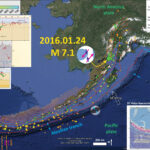
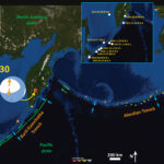
We just had an earthquake located along the Kamchatka Peninsula. Here is the USGS website for this M 7.2 earthquake. This earthquake was fairly deep and approximately east of a large and very deep earthquake from 2013. Here is my earthquake report for the 2013 M 8.3 earthquake and a second report for some triggered earthquakes updip of the M 8.3.
Below I present a summary poster for this earthquake. This earthquake appears to have occurred in the downgoing Pacific plate. Below is my interpretive poster where I plot the USGS moment tensor. This earthquake is an extensional earthquake with extension in the north-south direction. The downgoing plate experiences extension in two ways, from bending in the upper part of the plate and from tension due to slab pull (as the downgoing oceanic lithosphere is pulling the plate into the mantle). The orientation of the extension during this earthquake is interesting because it is not perpendicular to the plate boundary. The 2013.05.24 M 8.3 deep earthquake was oriented in the expected direction. I also include the region of Alaska that just had a M 7.1 earthquake. Here is my Earthquake Report for the Alaska earthquake.
I include labels for the plate boundary fault systems in the region and include generic focal mechanisms for these fault systems. There is a legend that shows how moment tensors can be interpreted. Moment tensors are graphical solutions of seismic data that show two possible fault plane solutions. One must use local tectonics, along with other data, to be able to interpret which of the two possible solutions is correct. The legend shows how these two solutions are oriented for each example (Normal/Extensional, Thrust/Compressional, and Strike-Slip/Shear). There is more about moment tensors and focal mechanisms at the USGS.
I include an inset map from the USGS (also included below). This map shows slip patches for some historic earthquakes. I used these slip patches to approximately place labels in green for these historic earthquakes.
I also include an inset map that shows the epicenters for historic earthquakes with USGS magnitudes greater than or equal to M 8.0. I label the dates and magnitudes of these earthquakes. Here is the query that I used to create this map. There is an interesting earthquake pair from 2006 and 2007. In 2006 there was a M 8.3 subduction zone earthquake that generated a Pacific-wide tsunami. The 2006 tsunami caused about $20 million in damage in Crescent City, CA. About a year later, there was a M 8.1 earthquake in the downgoing Pacific plate that was southeast of the trench. Dr. Erica Emery worked on this for her research.
Here is the tectonic summary poster from the USGS. This shows epicenters for earthquakes from 1900-2014, plus the slab contours from Hayes et al. (2012). These slab contours are estimate for the location of the subduction zone fault and it is based upon the 3-D location of earthquakes. There is considerable uncertainty with this model, but it is the best that we have. Hayes and his colleagues are currently updating these global slab models.
The USGS prepared a more comprehensive summary poster for this region. This poster has some plots of seismicity in cross sectional view. Here is the poster, but I include some sections of the poster below that are relevant for this earthquake.
Here is a map for the southern Kamchatka Peninsula. Earthquakes are plotted with diameter scaled to magnitude. The cross section C-C’ is labeled, as are the Hayes et al. (2012) slab contours. I place the epicenter for this earthquake as a green circle. The diameter is scaled approximately to magnitude and the location is approximate.
Here I place the hypocenter for this earthquake on the cross section from the USGS poster. The location is approximate.
Even though this is a very deep earthquake, due to its magnitude, it may lead to some casualties. Here is the PAGER alert, which is an estimate of the damage to people and their belongings (e.g. infrastructure). This is generated from a numerical model which overlays estimates of ground shaking with a geospatial database of people and infrastructure. This is only an estimate and it helps organizations plan for aid and assistance.
Here is a map from Lay et al. (2009) where they plot focal mechanisms for the 2006-2007 Kuril earthquake series. Note how the earthquakes in the Pacific plate are generally extensional. These earthquakes are in the outer rise, where the plate is flexed upward due to the forces exerted from subduction. The other interesting thing is that in 2009, there was a compressional earthquake in this same region. I include their figure caption as a blockquote.
Map showing regional bathymetry and tectonic features, along with global centroid moment tensor (CMT) solutions for the larger earthquakes in the 2006 –2007 Kuril Islands sequence (focal mechanisms), and NEIC epicenters of activity prior to the doublet (gray circles) between the two largest events (yellow circles), and following the 13 January 2007 event (orange circles). The gray shaded focal mechanisms are CMT solutions for foreshocks of the 15 November 2006 event, the red-shaded mechanisms occurred after the 15 November 2006 event, and events after 13 January 2008, including the trench slope 15 January 2009 event are green shaded. Focal mechanisms are plotted at the NEIC epicenters. The white stars indicate the CMT centroid locations for the two main shocks, which are shifted seaward relative to the NEIC locations. The arrow shows the estimated plate motion direction with a rate of 80 mm/yr computed using model NUVEL-1 [De Mets et al., 1990] with North America fixed.
Here is a map from Lay et al. (2009) that shows their interpretation of the tectonic regime of the outer rise of the Pacific plate prior to the 2006-2007 series. I include their figure caption as a blockquote.
Shallow seismicity distribution (NEIC epicenters) and all CMT solutions for events along the central Kuril Island region prior to the 15 November 2006 event. CMT centroid locations have an overall location bias somewhat toward the southeast. The approximate aftershock zones of the great 1963 Kuril Islands (Mw = 8.5) and 1952 Kamchatka (Mw = 9.0) earthquakes are outlined in red, and the epicenter of the 1915 (MS 8.0) event is shown by a red asterisk. The alongstrike extent of the 2006 –2007 great doublet is shown by the dashed red line with arrowheads. Outer rise activity of extensional or compressional nature is highlighted. The outer rise compressional mechanisms in red are from Christensen and Ruff [1988] with the 16 March 1963 event being labeled.
This shows their slip models for this earthquake pair, projected to the surface of the seafloor. I include their figure caption as a blockquote.
Surface map projection of coseismic slip for the 15 November 2006 (average slip 6.5 m) and the northwest dipping plane for 13 January 2007 (average slip 6.7 m at depths less than 25 km) events (NEIC epicenters, yellow circles, and CMT centroid epicenters, stars). Figure 15 indicates the relative position of the slip surfaces at depth. CMT mechanisms (centered on NEIC epicenters) for large events between June 2006 and May 2007 are shown; enlarged versions with first motions for the doublet events. Gray mechanisms indicate events before the 15 November 2006 event; red mechanisms indicate events after that rupture. The focal mechanism and epicenter of the 16 March 1963 (blue mechanism) and 15 January 2009 (green mechanism) compressional trench slope events (hexagons) are included. The arrow indicates the direction of the Pacific plate motion at 80 mm/yr.
Here Lay et al. (2009) present their interpretation for the earthquake cycle and how the tectonic regime changed during this period of a few decades. I include their figure caption as a blockquote.
Strain accumulation and release scenario for the great Kuril doublet. (a) During the interseismic period, the Pacific –North America (Okhotsk) plate interface is locked along the megathrust. Because of relative strength contrast between subducting and overriding plates, the elastic strain may preferentially accumulate within the elastic layer of the Pacific plate. Below the elastic layer, viscous strain accommodates the deformation and there is along-strike loading by underthrusting of the adjacent region of the arc. (b) During the 2006 earthquake, slip along the megathrust interface allows that segment of the Pacific plate to recover the accumulated slip deficit, and relaxation of accumulated compression or slab pull places the updip shallow region into an extensional strain environment causing the great 2007 extensional event. The region at the elastic-ductile transition (dotted line) deforms by viscous processes during the low strain rate interearthquake period, but will behave elastically during the high strain rate underthrusting event, helping to delay strain release in the overlying elastic lithosphere.
Following the earthquake pair today, I put together an animation showing the seismicity for this region between 1900 and 2016.01.30. I searched the USGS NEIC database for earthquakes of magnitude greater than or equal to M = 4.5. Here is my earthquake report for those earthquakes.
Here is a screenshot of the video.
Here is a download link for the video embedded below (2 MB mp4).
Here is my interpretive map for the two Gorda plate earthquakes.
NOAA Center for Tsunami Research just released an animation that shows a numerical simulation of what a tsunami may appear like when the next Cascadia subduction zone earthquake occurs. I present a summary about the CSZ tectonics on a 316th year commemoration page here. I include a yt link and embedded video and an mp4 embedded video and download link.
Here is a screenshot from the video:
There was just a pair of earthquakes near the Gorda rise. There was first an earthquake of magnitude M = 5.0, followed by a M = 4.9. The 5.0 appears to be within the GP, but the 4.9 seems to be at the eastern boundary of the ridge. These two earthquakes do not pose a tsunami risk for northern California (or elsewhere). Nor do they likely have an affect upon the likelihood of a Cascadia subduction zone earthquake.
**UPDATE: 2016.01.29 20:00 PST
The USGS has prepared a moment tensor for the M 5.0 earthquake. I have updated the map. It is clear now that this is an extensional (normal) earthquake. I include an updated map below the original map.
/end update
**UPDATE: 2023.01.29
The two events on this updated poster show how the faults near the spreading ridge are normal faults.
Below we see some maps showing how these normal faults, as the plate rotates in a clockwise fashion, also rotate. During this process, they are reactivated as left-lateral strike-slip faults.
Check out some of the earthquake reports for these strike-slip Gorda plate earthquakes listed at the bottom of this page. The 2014 M 6.8 event is a great example.
Here are the USGS web pages for these two earthquakes
Below is an interpretive map showing these two earthquakes as red circles, as well as other seismicity for the past week. I include an inset map of the Cascadia subduction zone (after Chaytor et al., 2004; Nelson et al., 2004), an inset map from Chaytor et al. (2004), and from Rollins and Stein (2010). I explain these inset maps below.
I include labels for the plate boundary fault systems in the region and include generic focal mechanisms for these fault systems. There is a legend that shows how moment tensors can be interpreted. Moment tensors are graphical solutions of seismic data that show two possible fault plane solutions. One must use local tectonics, along with other data, to be able to interpret which of the two possible solutions is correct. The legend shows how these two solutions are oriented for each example (Normal/Extensional, Thrust/Compressional, and Strike-Slip/Shear). There is more about moment tensors and focal mechanisms at the USGS.
Based on the locations of these earthquakes, along with our knowledge of the local tectonics, I interpret the M 5.0 to possibly be a northeast striking left-lateral strike-slip fault earthquake. The M 4.9 could either be like that, or be an extensional earthquake (like the 2014.03.13 earthquake listed below). I summarized the regional tectonics of the Cascadia subduction zone recently here. The M 5.0 earthquake is similar to the earthquake “P” on the Rollins and Stein (2010) map.
**UPDATE: 2016.01.29 20:00 PST
Here is the updated map. Note the extensional moment tensor. This is aligned nicely with the ridges from the Gorda rise (which are visible in the large scale map at the bottom of this page.
Here is a map of the Cascadia subduction zone, modified from Nelson et al. (2006). The Juan de Fuca and Gorda plates subduct norteastwardly beneath the North America plate at rates ranging from 29- to 45-mm/yr. Sites where evidence of past earthquakes (paleoseismology) are denoted by white dots. Where there is also evidence for past CSZ tsunami, there are black dots. These paleoseismology sites are labeled (e.g. Humboldt Bay). Some submarine paleoseismology core sites are also shown as grey dots. The two main spreading ridges are not labeled, but the northern one is the Juan de Fuca ridge (where oceanic crust is formed for the Juan de Fuca plate) and the southern one is the Gorda rise (where the oceanic crust is formed for the Gorda plate).
Here is a map from Chaytor et al. (2004) that shows some details of the faulting in the region. The moment tensor (at the moment i write this) shows a north-south striking fault with a reverse or thrust faulting mechanism. While this region of faulting is dominated by strike slip faults (and most all prior earthquake moment tensors showed strike slip earthquakes), when strike slip faults bend, they can create compression (transpression) and extension (transtension). This transpressive or transtentional deformation may produce thrust/reverse earthquakes or normal fault earthquakes, respectively. The transverse ranges north of Los Angeles are an example of uplift/transpression due to the bend in the San Andreas fault in that region.
Here is a map from Rollins and Stein, showing their interpretations of different historic earthquakes in the region. This was published in response to the Januray 2010 Gorda plate earthquake. The faults are from Chaytor et al. (2004).
Here is a large scale map of the region for these two earthquakes. This is taken from Google Earth. The two largest orange circles (color represents depth < 33 km) are the M 5.0 and M 4.9, with diameter representing magnitude. The M 5.0 is clearly in the region where there are north-northeast striking faults.
I have Earthquake Reports for other CSZ related earthquakes here:
Cascadia subduction zone
General Overview
1700.09.26 M 9.0 Cascadia’s 315th Anniversary 2015.01.26
1700.09.26 M 9.0 Cascadia’s 316th Anniversary 2016.01.26 updated in 2017 and 2018
Chaytor, J.D., Goldfinger, C., Dziak, R.P., Fox, C.G., 2004. Active deformation of the Gorda plate: Constraining deformation models with new geophysical data. Geology 32, 353-356.
Nelson, A.R., Kelsey, H.M., Witter, R.C., 2006. Great earthquakes of variable magnitude at the Cascadia subduction zone. Quaternary Research 65, 354-365.
Rollins, J.C., Stein, R.S., 2010. Coulomb Stress Interactions Among M ≥ 5.9 Earthquakes in the Gorda Deformation Zone and on the Mendocino Fault Zone, Cascadia Subduction Zone, and Northern San Andreas Fault. Journal of Geophysical Research 115, 19 pp.
In commemoration of the last known Cascadia subduction zone earthquake, I present a summary background material here. Since last years commemoration, there have been a few additions.
I made some updates on 2018.01.26.
Most notably was a pair of articles that were published in the New Yorker magazine, written by Kathryn Shulz. The first article summarized what we might expect from a CSZ earthquake and tsunami and the follow-up article discussed how to best prepare for this series of devastating events. The first article sparked a national debate after it was read by millions (using an estimate based upon the recorded time the website was being used). This debate has resulted in a renewed interest in becoming more resilient.
On this evening, 316 years ago, the Cascadia subduction zone fault ruptured as a margin wide earthquake. I here commemorate this birthday with some figures that are in two USGS open source professional papers. The Atwater et al. (2005) paper discusses how we came to the conclusion that this last full margin earthquake happened on January 26, 1700 at about 9 PM (there may have been other large magnitude earthquakes in Cascadia in the 19th century). The Goldfinger et al. (2012) paper discusses how we have concluded that the records from terrestrial paleoseismology are correlable and how we think that the margin may have ruptured in the past (rupture patch sizes and timing). The reference list is extensive and this is but a tiny snapshot of what we have learned about Cascadia subduction zone earthquakes. Brian Atwater and his colleagues have updated the Orphan Tsunami and produced a second edition available here for download and here for hard copy purchase (I have a hard copy).
This is a video from NOVA with the great Dr. Brian Atwater.
Here is a map of the Cascadia subduction zone, modified from Nelson et al. (2006). The Juan de Fuca and Gorda plates subduct norteastwardly beneath the North America plate at rates ranging from 29- to 45-mm/yr. Sites where evidence of past earthquakes (paleoseismology) are denoted by white dots. Where there is also evidence for past CSZ tsunami, there are black dots. These paleoseismology sites are labeled (e.g. Humboldt Bay). Some submarine paleoseismology core sites are also shown as grey dots. The two main spreading ridges are not labeled, but the northern one is the Juan de Fuca ridge (where oceanic crust is formed for the Juan de Fuca plate) and the southern one is the Gorda rise (where the oceanic crust is formed for the Gorda plate).
The USGS produces model based estimates for ground shaking using a variety of measures, for “scenario” earthquakes. Here is their website that explains this further. Below I present one of these scenarios, one for a M 9.0 CSZ eaarthquake. This is possibly what it was like for the last full rip CSZ earthquake on 1700.01.26.
USGS Shake Map M 9.0 Scenario Poster
In celebration of the anniversary in 2018, I prepared a new educational poster, which is based upon the above scenario shakemap.
I include some inset figures.
In the upper left corner is a map of the Cascadia subduction zone, modified from Nelson et al. (2004) and Chaytor et al. (2004).
Below the CSZ map is an illustration modified from Plafker (1972). This figure shows how a subduction zone deforms between (interseismic) and during (coseismic) earthquakes.
In the lower right corner is a figure from Atwater et al. (2005) that shows the earthquake cycle and how the crust deforms at different times.
On the left is the overall setting, where one plate subducts beneath another one at this compressional (convergent) plate boundary.
The center panel represents the interseismic period, the time between earthquakes. The fault is locked. The downgoing plate causes elastic strain to accumulate along the fault and in the two plates. The upper plate deforms vertically because of this. The region closest to the fault tip (the left) goes down and the part further from the fault tip goes up.
The right panel represents the coseismic period, when the earthquake happens. When the fault slips (in addition to some time before and after the earthquake), the upper plate deforms in an opposite sense of motion. This is the conventional view, but some say that because this system is not solely elastic (the mantle behaves with viscoelastic properties; Wang and Trehu, 2017).
Above this lower right corner figure is a figure from Atwater et al. (2005) that shows (A) how the vertical land motion produces earthquake stratigraphy in the form of buried soils (the trees died, so sad) and (B) a photo showing these buried soils, including a real dead tree stump (so sad).
In the upper right corner is a diagram that shows how we think the CSZ fault is segmented. Each segment is designated by an orange arrow. These orange arrows represent the region of the fault that has ruptured at different times. This is based upon turbidite stratigraphic correlations (Goldfinger et al., 2003, 2012, 2016). The yellow numbers represent the average time between earthquakes for each of these segments.
Dr. Nick Zentner (Central Washington Univ.) Video
CWU’s Nick Zentner presents ‘Great Earthquakes of the Pacific Northweset’ – the 13th talk in his ongoing Downtown Geology Lecture Series. Recorded at Hal Holmes Center on February 10, 2016 in Ellensburg, Washington, USA. www.nickzentner.com
IRIS / USGS Video
IRIS and the US Geological Survey have recently produced an educational video about tectonic earthquakes in the region of the US Pacific Northwest. The project was funded by the National Science Foundation. YT link for the embedded video below. mp4 link for the embedded video below.
mp4 embedded video:
YT embedded video:
I have compiled some literature about the CSZ earthquake and tsunami. Here is a short list that might help us learn about what is contained within the core that I collected.
This figure shows how a subduction zone deforms between (interseismic) and during (coseismic) earthquakes. We also can see how a subduction zone generates a tsunami. Atwater et al., 2005.
Here is a version of the CSZ cross section alone (Plafker, 1972).
Here is an animation produced by the folks at Cal Tech following the 2004 Sumatra-Andaman subduction zone earthquake. I have several posts about that earthquake here and here. One may learn more about this animation, as well as download this animation here.
This figure shows the regions that participate in this interseismic and coseismic deformation at Cascadia. Atwater et al., 2005. Black dots on the map show sites where evidence for coseismic subsidence has been found in coastal marshes, lakes, and estuaries.
This shows how the CSZ is deforming vertically today (Wang et al., 2003). The panel on the right shows the vertical motion in mm/yr.
This figure, also from Wang et al. (2003), shows their estimate of how the coseismic vertical motion may happen. Contours are in meters.
Here is a graphic showing the sediment-stratigraphic evidence of earthquakes in Cascadia. Atwater et al., 2005. There are 3 panels on the left, showing times of (1) prior to earthquake, (2) several years following the earthquake, and (3) centuries after the earthquake. Before the earthquake, the ground is sufficiently above sea level that trees can grow without fear of being inundated with salt water. During the earthquake, the ground subsides (lowers) so that the area is now inundated during high tides. The salt water kills the trees and other plants. Tidal sediment (like mud) starts to be deposited above the pre-earthquake ground surface. This sediment has organisms within it that reflect the tidal environment. Eventually, the sediment builds up and the crust deforms interseismically until the ground surface is again above sea level. Now plants that can survive in this environment start growing again. There are stumps and tree snags that were rooted in the pre-earthquake soil that can be used to estimate the age of the earthquake using radiocarbon age determinations. The tree snags form “ghost forests.
Here is a photo of the ghost forest, created from coseismic subsidence during the Jan. 26, 1700 Cascadia subduction zone earthquake. Atwater et al., 2005.
Here is a photo I took in Alaska, where there was a subduction zone earthquake in 1964. These tree snags were living trees prior to the earthquake and remain to remind us of the earthquake hazards along subduction zones.
This shows how a tsunami deposit may be preserved in the sediment stratigraphy following a subduction zone earthquake, like in Cascadia. Atwater et al., 2005. If there is a source of sediment to be transported by a tsunami, it will come along for the ride and possibly be deposited upon the pre-earthquake ground surface. Following the earthquake, tidal sediment is deposited above the tsunami transported sediment. Sometimes plants that were growing prior to the earthquake get entombed within the tsunami deposit.
The NOAA/NWS/Pacific Tsunami Warning Center has updated their animation of the simulation of the 1700 “Orphan Tsunami.”
Source: Nathan C. Becker, Ph.D. nathan.becker at noaa.gov
Here is the mp4 link for the embedded video below. (2160p 145 mb mp4)
Here is the mp4 link for the embedded video below. (1080p 145 mb mp4)
Here is the text associated with this animation:
Just before midnight on January 27, 1700 a tsunami struck the coasts of Japan without warning since no one in Japan felt the earthquake that must have caused it. Nearly 300 years later scientists and historians in Japan and the United States solved the mystery of what caused this “orphan tsunami” through careful analysis of historical records in Japan as well as oral histories of Native Americans, sediment deposits, and ghost forests of drowned trees in the Pacific Northwest of North America, a region also known as Cascadia. They learned that this geologically active region, the Cascadia Subduction Zone, not only hosts erupting volcanoes but also produces megathrust earthquakes capable of generating devastating, ocean-crossing tsunamis. By comparing the tree rings of dead trees with those still living they could tell when the last of these great earthquakes struck the region. The trees all died in the winter of 1699-1700 when the coasts of northern California, Oregon, and Washington suddenly dropped 1-2 m (3-6 ft.), flooding them with seawater. That much motion over such a large area requires a very large earthquake to explain it—perhaps as large as 9.2 magnitude, comparable to the Great Alaska Earthquake of 1964. Such an earthquake would have ruptured the earth along the entire length of the 1000 km (600 mi) -long fault of the Cascadia Subduction Zone and severe shaking could have lasted for 5 minutes or longer. Its tsunami would cross the Pacific Ocean and reach Japan in about 9 hours, so the earthquake must have occurred around 9 o’clock at night in Cascadia on January 26, 1700 (05:00 January 27 UTC).
The Pacific Tsunami Warning Center (PTWC) can create an animation of a historical tsunami like this one using the same too that they use for determining tsunami hazard in real time for any tsunami today: the Real-Time Forecasting of Tsunamis (RIFT) forecast model. The RIFT model takes earthquake information as input and calculates how the waves move through the world’s oceans, predicting their speed, wavelength, and amplitude. This animation shows these values through the simulated motion of the waves and as they race around the globe one can also see the distance between successive wave crests (wavelength) as well as their height (half-amplitude) indicated by their color. More importantly, the model also shows what happens when these tsunami waves strike land, the very information that PTWC needs to issue tsunami hazard guidance for impacted coastlines. From the beginning the animation shows all coastlines covered by colored points. These are initially a blue color like the undisturbed ocean to indicate normal sea level, but as the tsunami waves reach them they will change color to represent the height of the waves coming ashore, and often these values are higher than they were in the deeper waters offshore. The color scheme is based on PTWC’s warning criteria, with blue-to-green representing no hazard (less than 30 cm or ~1 ft.), yellow-to-orange indicating low hazard with a stay-off-the-beach recommendation (30 to 100 cm or ~1 to 3 ft.), light red-to-bright red indicating significant hazard requiring evacuation (1 to 3 m or ~3 to 10 ft.), and dark red indicating a severe hazard possibly requiring a second-tier evacuation (greater than 3 m or ~10 ft.).
Toward the end of this simulated 24-hours of activity the wave animation will transition to the “energy map” of a mathematical surface representing the maximum rise in sea-level on the open ocean caused by the tsunami, a pattern that indicates that the kinetic energy of the tsunami was not distributed evenly across the oceans but instead forms a highly directional “beam” such that the tsunami was far more severe in the middle of the “beam” of energy than on its sides. This pattern also generally correlates to the coastal impacts; note how those coastlines directly in the “beam” have a much higher impact than those to either side of it.
This is the timeline of prehistoric earthquakes as preserved in sediment stratigraphy in Grays Harbor and Willapa Bay, Washington. Atwater et al., 2005. This timeline is based upon numerous radiocarbon age determinations for materials that died close to the time of the prehistoric earthquakes inferred from the sediment stratigraphy at locations along the Grays Harbor, Willapa Bay, and Columbia River estuary paleoseismic sites.
Offshore, Goldfinger and others (from the 1960’s into the 21st Century, see references in Goldfinger et al., 2012) collected cores in the deep sea. These cores contain submarine landslide deposits (called turbidites). These turbidites are thought to have been deposited as a result of strong ground shaking from large magnitude earthquakes. Goldfinger et al. (2012) compile their research in the USGS professional paper. This map shows where the cores are located.
Here is an example of how these “seismoturbidites” have been correlated. The correlations are the basis for the interpretation that these submarine landslides were triggered by Cascadia subduction zone earthquakes. This correlation figure demonstrates how well these turbidites have been correlated. Goldfinger et al., 2012
This map shows the various possible prehistoric earthquake rupture regions (patches) for the past 10,000 years. Goldfinger et al., 2012. These rupture scenarios have been adopted by the USGS hazards team that determines the seismic hazards for the USA.
Here is a plot showing the earthquakes in a linear timescale.
I combined the plot above into another figure that includes all the recurrence intervals and segment lengths in a single figure. This is modified from Goldfinger et al. (2012), updated from new data (Goldfinger et al., 2016).
Social Media (2018 addition)
Today is the 318th anniversary of the Cascadia #earthquake of 1700. How do we know about #Cascadia's ancient earthquakes? Watch this video to find out! | VIDEO (00:03:54) Ghost Forests of the Pacific N.W.—Evidence for Cascadia's Past Earthquakes https://t.co/u6RcP9pMeNpic.twitter.com/RUSUWDQZSx
Viola Riebe, elder of the Hoh Indian Tribe, talks about an oral history of the Thunderbird and the whale — and how this most respected story is related to tsunami awareness. “We’re told in our language to run for high ground to get away from the ocean because it’s dangerous,” she says.
and here's a good piece from Hakai that summarizes some of the indigenous accounts in greater detail: https://t.co/NLeRySpTCA
Here is the Chaytor et al. (2004) map that shows their interpretation of the structural relations in the Gorda plate.
Here is a map from Rollins and Stein, showing their interpretations of different historic earthquakes in the region. This was published in response to the Januray 2010 Gorda plate earthquake. The faults are from Chaytor et al. (2004).
The Blanco fracture zone is also an active transform plate boundary. The BFZ is a strike slip fault system that connects two spreading ridges, the Gorda Rise and the Juan de Fuca Ridge. Here is a map that shows the tectonic setting and some earthquakes related to the BFZ from April 2015. There are some animations on this web page showing seismicity with time along the BFZ, over the past 15
years.
References
Atwater, B.F., Musumi-Rokkaku, S., Satake, K., Tsuju, Y., Eueda, K., and Yamaguchi, D.K., 2005. The Orphan Tsunami of 1700—Japanese Clues to a Parent Earthquake in North America, USGS Professional Paper 1707, USGS, Reston, VA, 144 pp.
Goldfinger, C., Nelson, C.H., Morey, A., Johnson, J.E., Gutierrez-Pastor, J., Eriksson, A.T., Karabanov, E., Patton, J., Gràcia, E., Enkin, R., Dallimore, A., Dunhill, G., and Vallier, T., 2012 a. Turbidite Event History: Methods and Implications for Holocene Paleoseismicity of the Cascadia Subduction Zone, USGS Professional Paper # 1661F. U.S. Geological Survey, Reston, VA, 184 pp.
McCrory, P.A., 2000, Upper plate contraction north of the migrating Mendocino triple junction, northern California: Implications for partitioning of strain: Tectonics, v. 19, p. 11441160.
McCrory, P. A., Blair, J. L., Oppenheimer, D. H., and Walter, S. R., 2006, Depth to the Juan de Fuca slab beneath the Cascadia subduction margin; a 3-D model for sorting earthquakes U. S. Geological Survey
Nelson, A.R., Kelsey, H.M., Witter, R.C., 2006. Great earthquakes of variable magnitude at the Cascadia subduction zone. Quaternary Research 65, 354-365.
Wang, K., Wells, R., Mazzotti, S., Hyndman, R. D., and Sagiya, T., 2003, A revised dislocation model of interseismic deformation of the Cascadia subduction zone Journal of Geophysical Research, B, Solid Earth and Planets v. 108, no. 1.
We just had a M 6.1 earthquake and a few aftershocks (M 4-5) in the western Mediterranean,
Here is the USGS website for this earthquake.
Here is a map showing the 5 largest earthquakes as circles.
There is a legend that shows how moment tensors can be interpreted. Moment tensors are graphical solutions of seismic data that show two possible fault plane solutions. One must use local tectonics, along with other data, to be able to interpret which of the two possible solutions is correct. The legend shows how these two solutions are oriented for each example (Normal/Extensional, Thrust/Compressional, and Strike-Slip/Shear). There is more about moment tensors and focal mechanisms at the USGS.
For more on the graphical representation of moment tensors and focal mechnisms, check this IRIS video out:
Based on the mapping presented by Gracia et al (2012), Casciello et al. (2016), and the bathymetry, this earthquake may have ruptured one of the northeast striking structures that are shown in the lower left part of the Gracia et al. (2012) map. Therefore I interpret this earthquake to be a left-lateral strike-slip earthquake.
Here is a close up of Gracia et al. (2012) Figure 1. I provide their caption below in blockquote.
Figure 1. Schematic geological map of the Westernmost Mediterranean highlighting the position of the Alboran Domain enclosed between Iberia and northwest Africa. Its metamorphic rocks compose the floor of the western Alboran Sea and form the inner zones of the Betics and Rif mountain chains.
Here is the Casciello et al (2016) figure showing their tectonic interpretation. Figure is their map and Figure 2 is an earlier tectonic interpretation (Andrieux et al., 1971). I provide their caption below in blockquote.
Fig. 1. Regional topographic and bathymetric map of the southeast Iberian margin constructed from digital grids released by SRTM-3, IEO bathymetry (Ballesteros et al., 2008; Mu˜noz et al., 2008) and MEDIMAP multibeam compilation (MediMap et al., 2008) at 90m grid-size. Epicenters of the largest historical earthquakes (MSK Intensity>VIII) in the region are depicted by a white star (I.G.N., 2010). Grey arrows pointing opposite each other show the direction of convergence between the Eurasian and African plates from NUVEL1 model (DeMets et al., 2010). The black outlined rectangle depicts the study area presented in Fig. 2. BSF: Bajo Segura Fault; AMF: Alhama de Murcia Fault, PF: Palomares Fault, CF: Carboneras Fault, YF: Yusuf Fault, AR: Alboran Ridge. Inset: Plate tectonic setting and main geodynamic domains of the south Iberian margin along the boundary between the Eurasian and African Plates.
Fig. 3. Original model by Andrieux et al. (1971) to explain the formation of the Gibraltar Arc. The Alboran microplate would resist the eastward movement of the European and African plates, which are
forced by oceanic expansion in the Atlantic, causing the formation of the Betic-Rif chains.
References:
Andrieux et al., 1971., Sur un modele explicatif de l’Arc de Gibraltar in Earth and Planetary Science Letters, v. 12, p. 191–198.
Early this morning, we had a M 7.1 earthquake in the Cook Inlet of Alaska. Here is the USGS web page for this earthquake. Due to the magnitude and depth for this earthquake, there is no tsunami risk for CA/OR/WA.
Below is a map that shows the seismicity from the past 30 days, with circles colored for depth (see legend). In the lower right corner is a map produced by Dr. Peter Haeussler from the USGS Alaska Science Center (pheuslr at usgs.gov) that shows the historic earthquakes along the Aleutian-Alaska subduction zone. I also plot the slab contours, which are lines that represent the depth of the subduction zone fault. These were constructed using seismicity and other sources of information from Hayes et al. (2012). There is considerable uncertainty for these contours, but they are the best information that we have about the location of the subduction zone fault. I also include an inset of part of the USGS Open File Report 2010-1083-B (Benz at al., 2010).
There is a legend that shows how moment tensors can be interpreted. Moment tensors are graphical solutions of seismic data that show two possible fault plane solutions. One must use local tectonics, along with other data, to be able to interpret which of the two possible solutions is correct. The legend shows how these two solutions are oriented for each example (Normal/Extensional, Thrust/Compressional, and Strike-Slip/Shear). There is more about moment tensors and focal mechanisms at the USGS.
This is an interesting earthquake. The depth (~128 km) aligns with the slab contours. This means that we could interpret this to be a subduction zone earthquake. Note how this earthquake is northwest of the 1964 Good Friday earthquake. This earthquake is down-dip from slip during that 27 March 1964 M 9.2 earthquake. I plot the epicenter on the Benz et al. (2010) map and the hypocenter along the cross section from Benz et al. (2010) as red circles. This earthquake occurred in the downgoing Pacific plate.
This is the visualized ground motion recorded in Homer, AK from the M7.1 Alaska earthquake on January 24, 2016. High pass filtered at 0.1Hz. Made with SeismoVisualize.
Here is a link to download the embedded video below (8 MB mp4).
Here is a map for the earthquakes of magnitude greater than or equal to M 7.0 between 1900 and today. This is the USGS query that I used to make this map. One may locate the USGS web pages for all the earthquakes on this map by following that link.
Here is a map that shows the regional extent of the 1964 earthquake. Regions of coseismic uplift/subsidence are delineated by blue/red polygons.
This animation shows the underlying causes of that earthquake, and tells how research done on the ground deformation contributed to confirmation of early theories of plate tectonics. More background material about this animation is found here. Here is a download link for the embedded video below (85 MB mp4).
Here is a large scale map (zoomed in) for the local scale, showing the main shock and the aftershocks. These aftershocks show an east-northeast trend.
Dr. Peter Haeussler produced a cross section for this region. Below is his description of this figure.
I made up a quick diagram (thanks Alaska Earthquake Center tools) showing the tectonic setting of the earthquake. This was a “Benioff zone” event, which means that the earthquake is related to bending of the subducting Pacific Plate as it slides into the mantle.
More interesting thoughts. Many earthquakes that are due to bending of the downgoing slab are in the upper part of the downgoing plate and these earthquakes are extensional due to the extension in the upper part of the plate due to the bending. Well, the opposite happens on the lower part of the bending plate. This is what happened during this M 7.1 earthquake, it is a compressional earthquake (in addition to the strike-slip part).
Here is a plot of static displacements for GPS sites as modeled by Jeff Freymueller at University of Alaska, Fairbanks (jeff.freymueller at gi.alaska.edu).
Here is the seismic record from Homer, AK. This was tweeted by Andy Frassetto at IRIS.
Here is an animation from Matt Gardine, showing ug PGA (500 = 0.5 PGA) measured at different locations.
I put together an animation of the seismicity for this region from the period of 1900-2016, for earthquakes of magnitude greater than or equal to M 6.5. Below is a map showing all these earthquakes and below that is the animation.
Here is a link to the embedded video below (25 MB mp4) .
Here is a map that shows the seismicity (1960-2014) for this plate boundary. This is the spatial extent for the video below.
Here is a link to the file to save to your computer.
Here is a map showing the shaking intensity that uses the Modified Mercalli Intensity (MMI) scale. The MMI scale is a qualitative scale of the ground motions. There is more about the MMI here.
The USGS has prepared a fault slip model.
Today’s earthquake occurred near the inferred segment boundary between the locked Kodiak and creeping Kenai segments of the megathrust. Here is a map from Kelsey et al. (2015). They were looking at beach ridges on the Kenai penninsula, which are unrelated to this M 7.1 earthquake. I include the figure caption for part A, below as a blockquote.
A. Tectonic setting of the eastern Alaska-Aleutian subduction zone megathrust. Bold line delineates the surface trace of the megathrust, barbs on upper (North American) plate. Vertical deformation during the 1964 great Alaska earthquake depicted by two adjoining margin-parallel belts: a region of landward subsidence (blue) and a region of seaward uplift (red) (Plafker, 1969). Areas of highest slip occurred below the Prince William Sound and Kodiak segments, which are currently locked currently; while the intervening Kenai segment is creeping presently (Freymueller et al., 2008).
Based upon their work, they interpret that there may or may not be a segment boundary in this location (Kelsey et al., 2015).
Three alternatives for the tectonic context of the penultimate AD 1530-1840 Kenai earthquake in comparison to the AD 1964 earthquake and the third oldest earthquake. A. Coseismic uplift extent of the AD 1964 earthquake on which is superposed the inferred coseismic uplift extent of the AD 1788 rupture, if this historic earthquake involved rupture of the Kenai segment (alternative A). The colors show geodetic coupling ratio units as a fraction of the contemporary Pacific-North American plate rate, taken from Zweck et al., 2002. B. Alternative B (yellow) is the inferred uplift extent of the AD 1430-1650 subduction zone earthquake if this earthquake involved rupture of the Kenai segment. Alternative C (red) is the inferred uplift extent of the penultimate Kenai earthquake if earthquake rupture involved the Kenai segment alone. C. Inferred uplift extent for the ~900 cal yr BP earthquake, which is recorded in Prince William Sound, on the Kenai Peninsula (this study) as well as on Kodiak and Sitkinak Islands.
The NOAA/NWS/Pacific Tsunami Warning Center has updated their animation of the simulation of the 1700 “Orphan Tsunami.”
Source: Nathan C. Becker, Ph.D. nathan.becker at noaa.gov
I provide some other background information about Cascadia here:
Here is the mp4 link for the embedded video below. (2160p 145 mb mp4)
Here is the mp4 link for the embedded video below. (1080p 145 mb mp4)
Here is the text associated with this animation:
Just before midnight on January 27, 1700 a tsunami struck the coasts of Japan without warning since no one in Japan felt the earthquake that must have caused it. Nearly 300 years later scientists and historians in Japan and the United States solved the mystery of what caused this “orphan tsunami” through careful analysis of historical records in Japan as well as oral histories of Native Americans, sediment deposits, and ghost forests of drowned trees in the Pacific Northwest of North America, a region also known as Cascadia. They learned that this geologically active region, the Cascadia Subduction Zone, not only hosts erupting volcanoes but also produces megathrust earthquakes capable of generating devastating, ocean-crossing tsunamis. By comparing the tree rings of dead trees with those still living they could tell when the last of these great earthquakes struck the region. The trees all died in the winter of 1699-1700 when the coasts of northern California, Oregon, and Washington suddenly dropped 1-2 m (3-6 ft.), flooding them with seawater. That much motion over such a large area requires a very large earthquake to explain it—perhaps as large as 9.2 magnitude, comparable to the Great Alaska Earthquake of 1964. Such an earthquake would have ruptured the earth along the entire length of the 1000 km (600 mi) -long fault of the Cascadia Subduction Zone and severe shaking could have lasted for 5 minutes or longer. Its tsunami would cross the Pacific Ocean and reach Japan in about 9 hours, so the earthquake must have occurred around 9 o’clock at night in Cascadia on January 26, 1700 (05:00 January 27 UTC).
The Pacific Tsunami Warning Center (PTWC) can create an animation of a historical tsunami like this one using the same too that they use for determining tsunami hazard in real time for any tsunami today: the Real-Time Forecasting of Tsunamis (RIFT) forecast model. The RIFT model takes earthquake information as input and calculates how the waves move through the world’s oceans, predicting their speed, wavelength, and amplitude. This animation shows these values through the simulated motion of the waves and as they race around the globe one can also see the distance between successive wave crests (wavelength) as well as their height (half-amplitude) indicated by their color. More importantly, the model also shows what happens when these tsunami waves strike land, the very information that PTWC needs to issue tsunami hazard guidance for impacted coastlines. From the beginning the animation shows all coastlines covered by colored points. These are initially a blue color like the undisturbed ocean to indicate normal sea level, but as the tsunami waves reach them they will change color to represent the height of the waves coming ashore, and often these values are higher than they were in the deeper waters offshore. The color scheme is based on PTWC’s warning criteria, with blue-to-green representing no hazard (less than 30 cm or ~1 ft.), yellow-to-orange indicating low hazard with a stay-off-the-beach recommendation (30 to 100 cm or ~1 to 3 ft.), light red-to-bright red indicating significant hazard requiring evacuation (1 to 3 m or ~3 to 10 ft.), and dark red indicating a severe hazard possibly requiring a second-tier evacuation (greater than 3 m or ~10 ft.).
Toward the end of this simulated 24-hours of activity the wave animation will transition to the “energy map” of a mathematical surface representing the maximum rise in sea-level on the open ocean caused by the tsunami, a pattern that indicates that the kinetic energy of the tsunami was not distributed evenly across the oceans but instead forms a highly directional “beam” such that the tsunami was far more severe in the middle of the “beam” of energy than on its sides. This pattern also generally correlates to the coastal impacts; note how those coastlines directly in the “beam” have a much higher impact than those to either side of it.
We just had an earthquake offshore of Colima, Mexico. This earthquake appears associated with the Rivera fracture zone (RFZ), a transform plate boundary separating the Rivera plate to the north and the Pacific plate to the south. The RFZ connects segments of the East Pacific Rise, the oceanic spreading center where the Pacific plate, Rivera plate, and Cocos plate are formed. The RFZ is a system of stepped right lateral strike-slip faults. There is likely zero risk of a tsunami from this strike-slip earthquake. Here is the USGS web site for this earthquake.
Below is a map showing the regional tectonics. I made this using Google Earth ™. The seismicity from the last 30 days (USGS feed) is plotted vs. depth (color, see legend on left).
There is a legend that shows how moment tensors can be interpreted. Moment tensors are graphical solutions of seismic data that show two possible fault plane solutions. One must use local tectonics, along with other data, to be able to interpret which of the two possible solutions is correct. The legend shows how these two solutions are oriented for each example (Normal/Extensional, Thrust/Compressional, and Strike-Slip/Shear). There is more about moment tensors and focal mechanisms at the USGS.
Based on the location of this earthquake (adjacent to the RFZ), I interpret this to be a right lateral (dextral) strike slip earthquake.
I plate some inset maps to help with the tectonic interpretation from Blatter and Hammersley (2010) and Gaviria et al. (2013).
For more on the graphical representation of moment tensors and focal mechnisms, check this IRIS video out:
This earthquake was not felt much in Mexico, based upon these USGS “Did You Feel It?” reports.
Gaviria et al. (2013) use magnetic anomalies to interpret the very complicated tectonics at the eastern part of the RFZ. Here is their plate tectonic map.
This map includes focal mechanisms for earthquakes in the region. This helps them interpret the faulting.
Here is their figure showing the bathymetry of the region, along with their interpretation of where different fault systems are.
Here is the linework showing just the anomalies and faults.
This map shows their interpretation for the development of the plate boundary from 3-1 Ma.
Today there was a bantering about a buoy several hundred miles offshore of Oregon. A website had posted a hoax about how the buoy data suggested that there was movement along the Cascadia subduction zone. These hoaxes happen rather frequently. One of the most famous hoaxsters has an online name that rhymes with munchkins. In addition to my post here, my good friend from southern Oregon shared me this link, where Scott Burns also debunks this hoax.
Here I present some screen shots from this hoax website. I spend more time helping people learn how to tell the difference between credible sources of information and non-credible sources of information on my Fukushima page here. Basically, sometimes it is difficult to really know if a source of information is credible or not, especially if we are not experts in that field. I use the Fukushima fear example and today’s example to debunk these non-credible sources since I am more informed about these topics. I do not provide a link to the ss95 page because I do not want them to make any more money on this hoax. If you do go there, you will find a plethora (thanks Tom H. Leroy, the man with four first names, for the word of the day) of other web pages that are equally annoying and hoaxes. Red flags!
There are many websites that are probably not good sources of information (duh!). When they have crazy names, like superstation95, it is probably a good bet that they are not credible sources of information. Here is a pdf of the ss95 page as I went to press. They edited the page several times since I first saw it this morning. I wonder why (not really, they are cleaning up their misinformation slightly).
Here is the top of this page that is clearly full of misinformation. I will briefly review some of this misinformation. I grabbed these screen shots about 18:50 on 2016.01.18.
There is a statement “the land beneath the ocean has suddenly “sunk”.” The buoy is located several hundred nautical miles west of Astoria. This is quite far from the Cascadia subuction zone (CSZ) and if the CSZ were to deform the sea floor, this buoy would absolutely not observe nor record that.
Another statement, “An ocean data buoy is alerting to an “event”.” These buoys have algorithms that find excursions in the data and identify them as “events” so that a real person can review these data to see if something is happening. The fact that there are “events” only signifies that there is an excursion. I will review this excursion below.
Here is the next part of this ss95 hoax. These are plots from the Buoy web page here. If one clicks on “Data Type” and select “events,” they can choose from the different events. This link already shows the “event” that is plotted below.
The upper panel shows a 5 minute period (the excursion) and the lower panel shows a 5 hour period of time, with the excursion highlit in red. Note the vertical scale on both plots. The upper plot shows a peak-to-trough distance of 6 cm (the units are meters; 2738.72-2738.66 = 6 cm). This would generally be considered a 3 cm wave height. NOT VERY SIGNIFICANT. The lower panel shows that there are many waves before and after the excursion that look to have amplitudes very similar to this excursion. This is because these are all simply typical ocean waves. About 20 minutes after the excursion is another wave that is almost the same size, just before 03 GMT.
They claim that “The [E]arth sunk.” Anyone who does not capitalize the “E” in Earth… well, I am not the capitalization police… but it does not support this source as being credible. Again, this buoy is not located above the CSZ, so could not move due to deformation along the CSZ.
The claim, “The buoy is too far away from shore to be affected by high/low tide, so where did the four feet of ocean water disappear to?”
This is patently false. I post a great graphic from NOAA below. Tides occur here as much as they do anywhere else (there are places where tides are greater and lesser, but that is not really relevant to debunk their false statement).
Where did they come up with 4′ of water? Oh, the tides. I thought that they were talking about the “event” wave, which only has a much much smaller amplitude. Their hoax web page is really confusing. This should be a red flag.
They state the following:
This means a Tectonic Plate in the Ocean named the “Juan de Fuca Plate” has made a sudden, eastward movement and slipped beneath another Tectonic Plate named the “North American Plate.” This type of event is usually followed by a massive upward movement of the North American Plate causing a very severe earthquake.
This Buoy is over the Juan de Fuca plate. We can give them that. The JDF plate will go eastward during a subduction zone earthquake. Sure. There will be vertical deformation of the sea floor during a CSZ earthquake, just not in the location of the buoy.
Here is a map showing the buoy’s location (station 46404). The largest yellow diamond is the location of the buoy. The Juan de Fuca Ridge is to the west of this Buoy and the CSZ is farrrrr to the east. Remember, this buoy is 230 nautical miles (a nm = 1.852 km, while a mile is 1.6 km) from Astoria, at the mouth of the Columbia River.
Here is the NOAA tides infographic. Thanks NOAA Twitter Feed!
If you are concerned about tsunamis, there are only a few things that you need to know.
If you live along the coast and the CSZ earthquake happens, which will generate a tsunami, the ground shaking is your “Natural Warning.” You do not need to wait for anything else to evacuate to high ground for a tsunami evacuation site. You can do it on your own!
If there is a tsunami coming from an earthquake from elsewhere in the Pacific, there will be many different kinds of warnings (from helicopters, to sirens, to email and other media alerts). You can sign up for notifications from NOAA.
For example, here is the screen shot from the NOAA/NWS National Tsunami Warning Center.
Remember, the I-5 is not a geological boundary. There will NOT be a 45′ tall tsunami passing Interstate 5. There will not be a tsunami in Portland. Ground shaking sure, but no tsunami.
It has been hypothesized that subduction zone earthquakes can change the stresses in magma chambers, leading to volcanic eruptions. For example, it has been reasoned (in a peer review journal article) that a volcano erupted in Alaska following the 2004 Sumatra-Andaman subduction zone earthquake. However, the source of heat that leads to the melting of oceanic lithosphere is NOT from the friction along the fault (but from the mantle, sourced from the original Earth and ongoing radioactive decay within the Mantle). This should be another red flag. Also, when this molten rock is beneath the Earth, it is called magma, not lava. More red flags. IF any of the Cascades range volcanoes were to erupt following a CSZ earthquake, we would most likely know about this long before it were to happen.