I was slowly waking up while looking at my social media feed. moments before (maybe minutes) Anthony Lomax had posted his first motion earthquake mechanism for a M 6.4 near the CA/NV border. I leaped out of bed and got off a map before i had the time to put any clothes on (one benefit of teleworking that i won’t go into too many details).
https://earthquake.usgs.gov/earthquakes/eventpage/nn00725272/executive
There was a swarm of earthquakes east of Mono Lake in April along the Huntoon Valley fault zone. These events are aligned with faults that trend east-northeast. The plate boundary relative plate motion is generally aligned with the San Andreas fault system (north-northwest trending right-lateral strike-slip faulting). To the east, tectonics are dominated by ~east-west extension in the Basin and Range geomorphic province.
As the plate boundary organizes itself along the east side of the Sierra Nevada, it has some disruptions, with blocks that are rotating in ways (within this right-lateral shear) that lead to these northeast trending faults.
As the blocks rotate, the faults that bound these blocks (the east-northeast faults) are left-lateral strike-slip faults. More on this below.
In April these earthquakes were along some of these east-northeast left-lateral faults, with the largest magnitude = M 5.2. Today’s ongoing sequence is to the east along the same trend of faulting, along faults mapped by Tom Sawyer of Piedmont Geosciences called “unnamed faults of the Candelaria Hills.”
It seems hard to believe that these earthquakes are unrelated. They are within about a month of each other. They are along the same fault system.
Taking this thought experiment through, it seems that an earthquake could happen between these earthquakes along this fault system.
Using Wells and Coppersmith (1994) empirical relations between surface rupture length (the length of the fault that would break through the ground surface) and earthquake magnitude can help us estimate what magnitude of an earthquake may be given a rupture length.
If we use these relations, and the distance between these earthquakes, we measure a distance of 50 km and can calculate a magnitude of M 7.0. Thus, it would be prudent for people in the region to stay safe and ensure that they are prepared for a potentially larger earthquake.
There is an alternate explanation for today’s sequence. The M 6.4 was on a north-south oriented fault and was right-lateral strike-slip, while many of the aftershocks are actually instead triggered earthquakes on the east-west trending left-lateral strike-slip earthquake fault system. Which recent earthquake sequence had two almost perpendicularly relative orientations? Yes, the Ridgecrest Earthquake Sequence. Now, this is a more complicated explanation, but it is possible (tho at this point, i deem it unlikely).
UPDATE 16 MAY
Reports from the field are that the surface rupture is north-south just east of Rock Hill (feature shown on USGS earthquake event page web map). Rock Hill is west of the M 6.5 epicenter, and just east of HWY 95 38.149 N 117.941 W. Observations from Jamie Shutmut.
perhaps the alternate hypothesis mentioned last night was the correct hypothesis?
UPDATE later
There have been many different observations in the field to suggest that the surface deformation from this event sequence is broadly distributed and the offsets at the surface are on the order of centimeters, maybe a half a decimeter.
It appears that the main fault was ~east-west, but that there may be some north-south structure involved too.
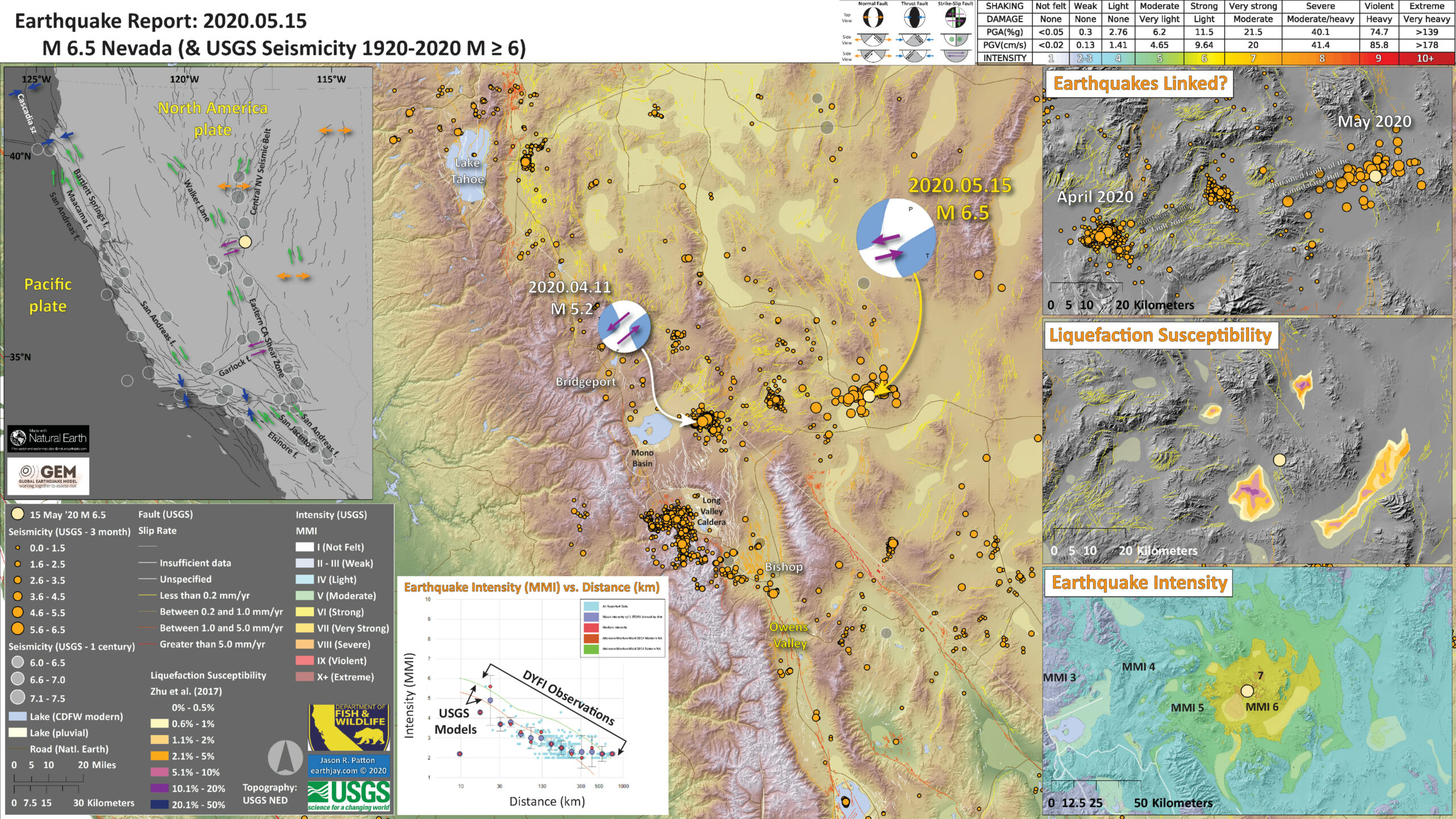
Below is my interpretive poster for this earthquake
- I plot the seismicity from the past 3 months, with diameter representing magnitude (see legend). I include earthquake epicenters from 1920-2020 with magnitudes M ≥ 6.0 in one version.
- I plot the USGS fault plane solutions (moment tensors in blue and focal mechanisms in orange), possibly in addition to some relevant historic earthquakes.
- A review of the basic base map variations and data that I use for the interpretive posters can be found on the Earthquake Reports page.
- Some basic fundamentals of earthquake geology and plate tectonics can be found on the Earthquake Plate Tectonic Fundamentals page.
- In the upper left corner is a small scale (zoomed out) view of the western USA showing the major tectonic faults (from the Global Earthquake Model). I show USGS seismicity from the past century.
- In the lower right corner is a map showing the earthquake intensity using the Modified Mercalli Intensity Scale (MMI) as modeled by the USGS.
- In the upper right corner is a map that shows the earthquakes from the past month. Note how the April sequence is related to today’s ongoing sequence.
- In the center right is a map that shows the liquefaction susceptibility model from the USGS. This is a model and not based on direct observation, however, it could be used to help direct field teams to search for this type of effect.
- In the lower center is a plot showing how shaking intensity lowers with distance from the earthquake. The models that were used to produce the Earthquake Intensity map to the right are the same model results represented by the orange and green lines. However, on this plot, there are also observations from real people! The USGS Did You Feel It? questionnaire lets people report their observations from the earthquake and these data are plotted here. We can then compare the model with the observations.
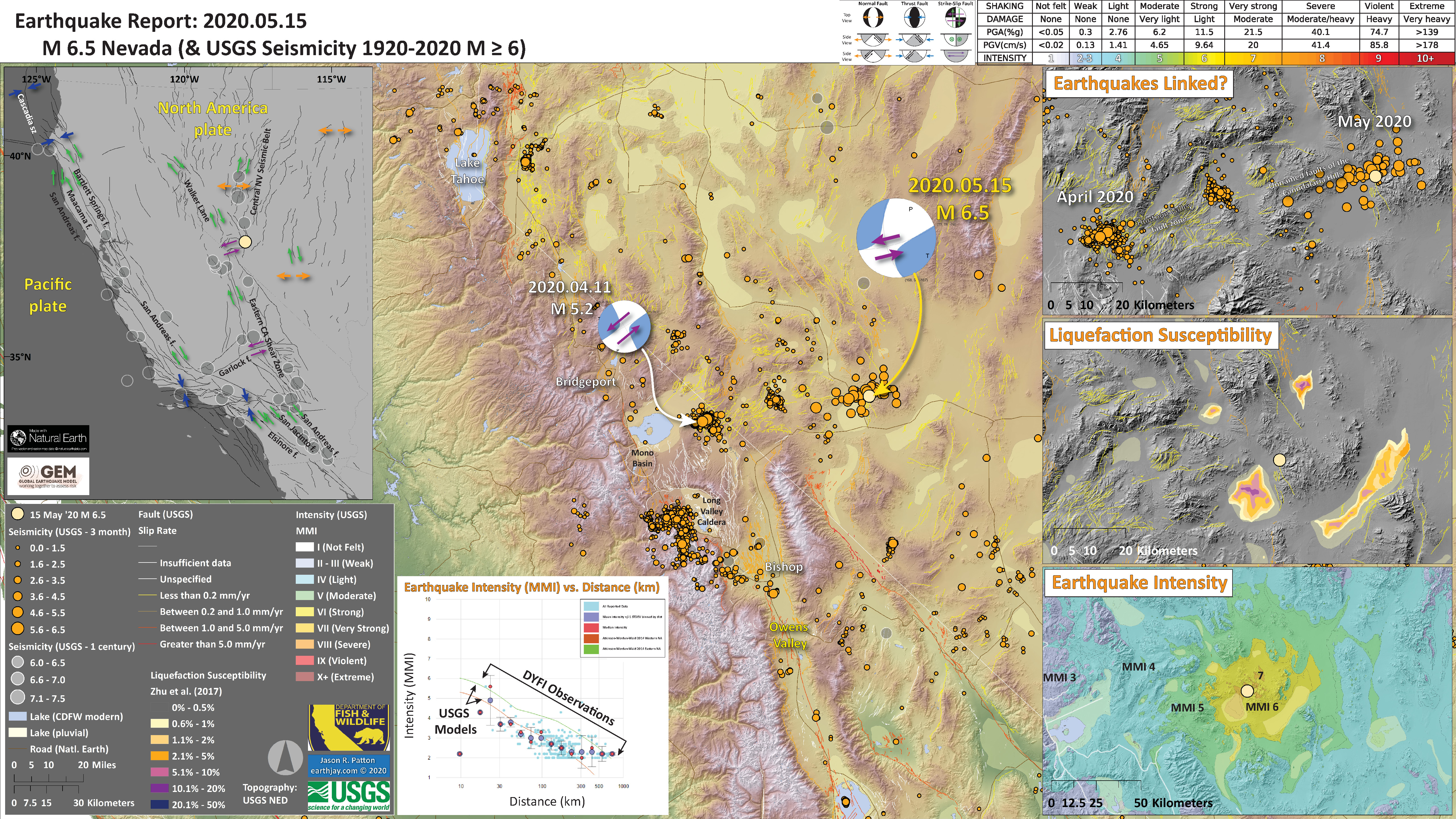
I include some inset figures. Some of the same figures are located in different places on the larger scale map below.
- Here is the map with 3 month’s seismicity plotted.
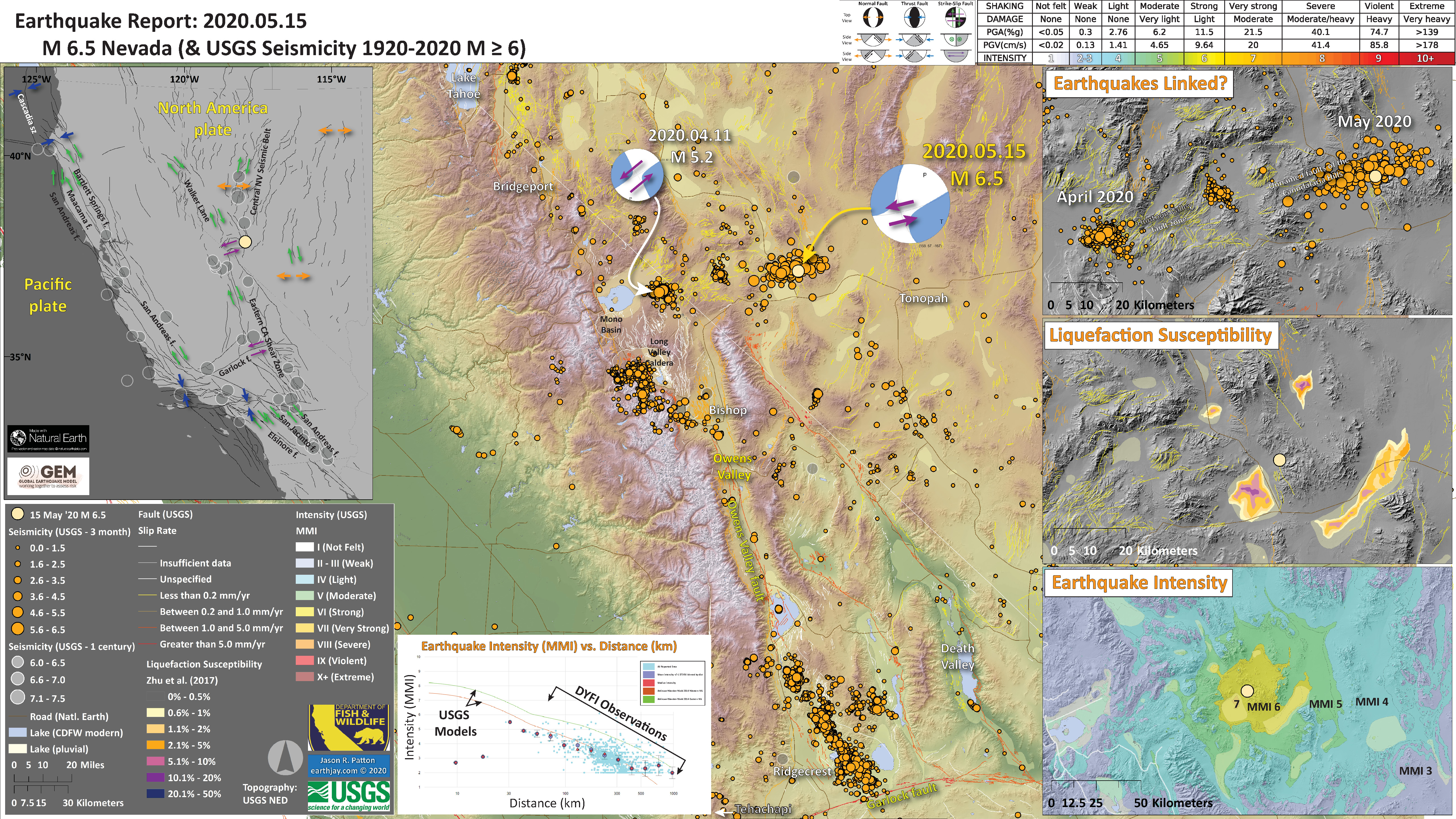
- An update from this evening (some changes in intensities). I moved the map to include aftershocks from the Ridgecrest Earthquake Sequence.
- I also had forgotten to label Tonopah, so needed to add a label for Tehachapi too.
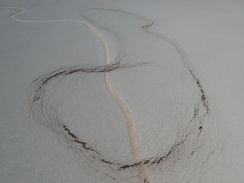
- Here are some photos from Jamie Shutmutt which are in the social media section below.
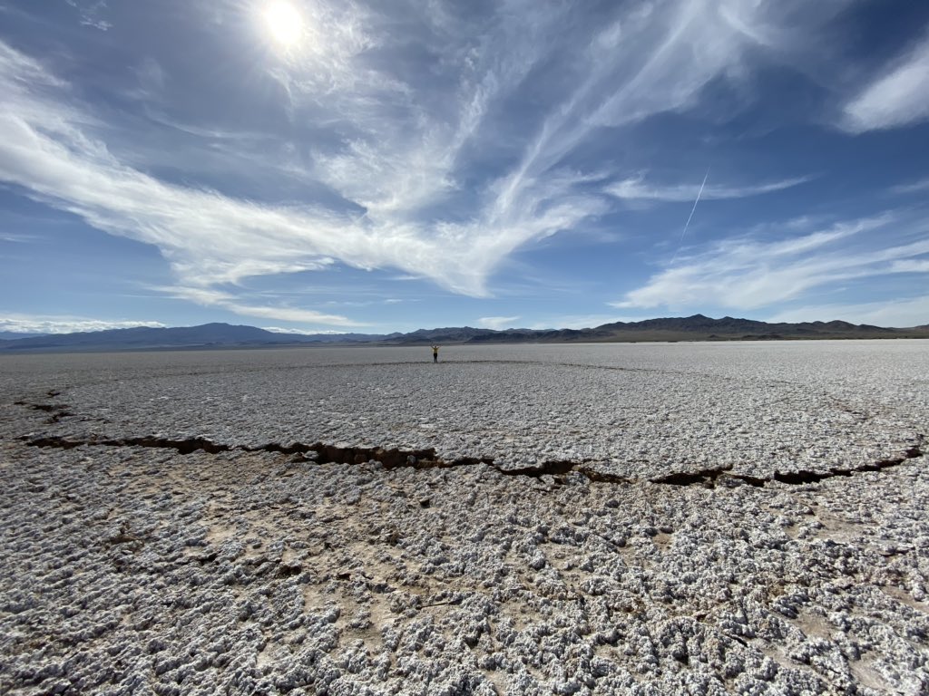
- These two images show evidence of ground disruption. This is likely the result of liquefaction in the subsurface. There are varying hypotheses about how this specifically happens, but it is basically the result of water pressure pushing against the sediment particles so that they move like fluid.
- Sediment or soil strength is based upon the ability for sediment particles to push against each other without moving. This is a combination of friction and the forces exerted between these particles. This is loosely what we call the “angle of internal friction.” Liquefaction is a process by which pore pressure increases cause water to push out against the sediment particles so that they are no longer touching.
- An analogy that some may be familiar with relates to a visit to the beach. When one is walking on the wet sand near the shoreline, the sand may hold the weight of our body generally pretty well. However, if we stop and vibrate our feet back and forth, this causes pore pressure to increase and we sink into the sand as the sand liquefies. Or, at least our feet sink into the sand.
- Below is a diagram showing how an increase in pore pressure can push against the sediment particles so that they are not touching any more. This allows the particles to move around and this is why our feet sink in the sand in the analogy above. This is also what changes the strength of earth materials such that a landslide can be triggered.
- During our post earthquake response to the Ridgecrest Earthquake Sequence in July of 2019, we observed similar features in places like in the Salt Wells Valley playa.
- Take a look at the earthquake report interpretive poster above for today’s M 6.5 earthquake. Look at the liquefaciton susceptibility map. Can you tell where these photos may have been taken?
- Yes, that’s right! These photos were taken in the area to the west of the epicenter. Note the north-south highway west of the M 6.5 epicenter. This is HWY 95 and the playa to the west shows a high chance of liquefaction, right where these photos were taken.

- Here is the poster for the earthquakes in April 2020.

USGS Shaking Intensity
- UPDATE:evening of 15 May
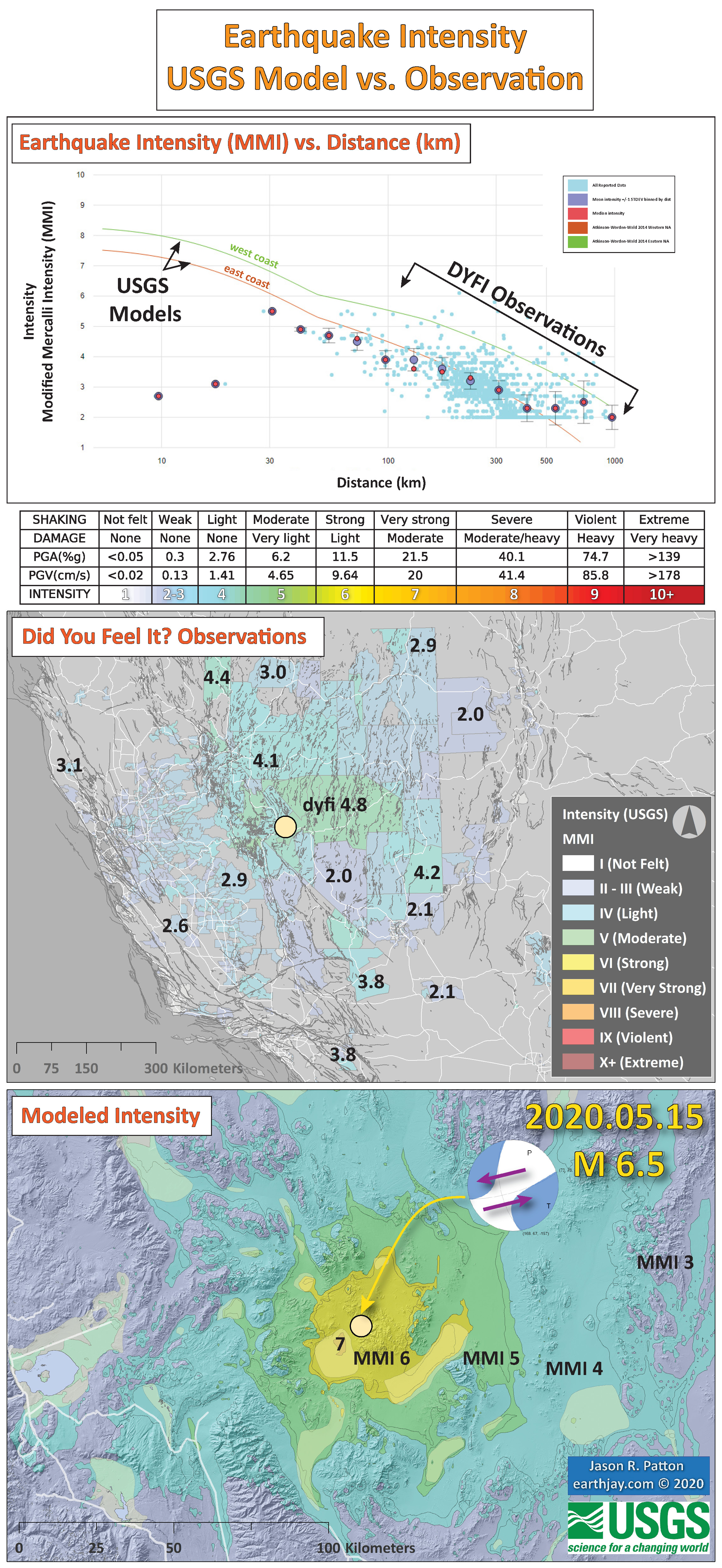
- Here is a figure that shows a more detailed comparison between the modeled intensity and the reported intensity. Both data use the same color scale, the Modified Mercalli Intensity Scale (MMI). More about this can be found here. The colors and contours on the map are results from the USGS modeled intensity. The DYFI data are plotted as colored dots (color = MMI, diameter = number of reports).
- In the upper panel is a plot showing MMI intensity (vertical axis) relative to distance from the earthquake (horizontal axis). The models are represented by the green and orange lines. The DYFI data are plotted as light blue dots. The mean and median (different types of “average”) are plotted as orange and purple dots. Note how well the reports fit the green line (the model that represents how MMI works based on quakes in California).
- Below the upper panel plot is the USGS MMI Intensity scale, which lists the level of damage for each level of intensity, along with approximate measures of how strongly the ground shakes at these intensities, showing levels in acceleration (Peak Ground Acceleration, PGA) and velocity (Peak Ground Velocity, PGV).
- In the center panel is the USGS Did You Feel It reports map, showing reports as colored dots using the MMI color scale.
- In the lower panel is the map that shows the modeled intensity using the same model that is plotted in the upper panel.
Other Report Pages
Some Relevant Discussion and Figures
- Here are the two figures from Rinke et al. (2012) that show the global and regional tectonics here. I include the figure captions below as blockquotes. The first map shows the plate boundary scale tectonic regions. This is a generalized map (e.g. don’t pay attention to where the San Andreas and Cascadia faults are located). The second map shows the regional fault systems.
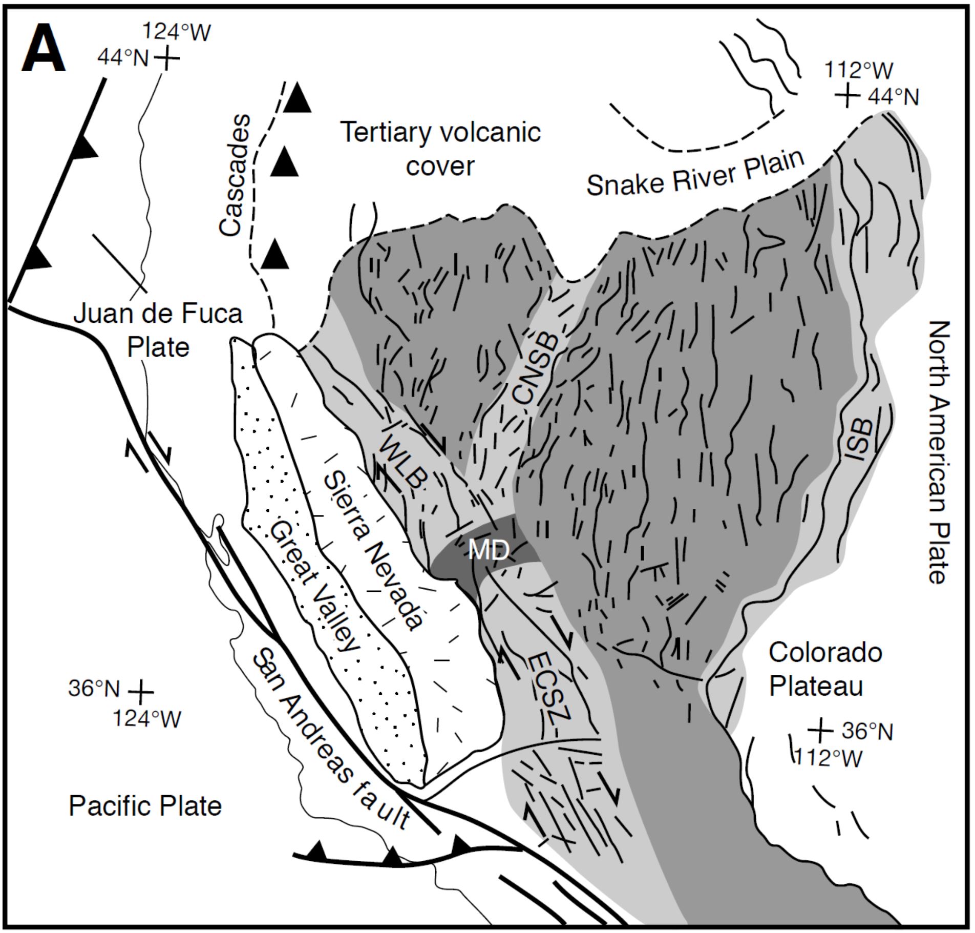
Simplified tectonic map of the western U.S. Cordillera showing the modern plate boundaries and tectonic provinces. Basin and Range Province is in medium gray; Central Nevada seismic belt (CNSB), eastern California shear zone (ECSZ), Intermountain seismic belt (ISB), and Walker Lane belt (WLB) are in light gray; Mina deflection (MD) is in dark gray.
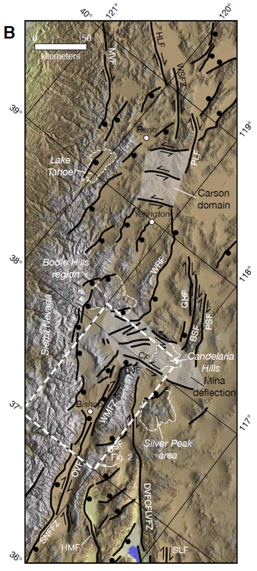
Shaded relief map of the WLB and northern part of the ECSZ showing the major Quaternary faults. Solid ball is located on the hanging wall of normal faults; arrow pairs indicate relative motion across strike-slip faults; white dashed box outlines location of Figure 2; light gray shaded areas show the Mina deflection and the Carson domain. BSF—Benton Springs fault; CF—Coaldale fault; DSF—Deep Springs fault; DVFCFLVFZ—Death Valley–Furnace Creek–Fish Lake Valley fault zone; GHF—Gumdrop Hills fault; HLF—Honey Lake fault; HMF—Hunter Mountain fault; MVF—Mohawk Valley fault; OVF— Owens Valley fault; PLF—Pyramid Lake fault; PSF—Petrified Springs fault; QVF—Queen Valley fault; SLF—Stateline fault; SNFFZ—Sierra Nevada frontal fault zone; WMFZ—White Mountains fault zone; WRF—Wassuk Range fault; WSFZ—Warm Springs fault zone.
- Here is a figure from Wesnousky et al. (2012) where a wax block model is used to illustrate their interpretations of the tectonic deformation along the Walker Lane region. Today’s earthquakes occurred in the basin to the west of the circled number “7.”
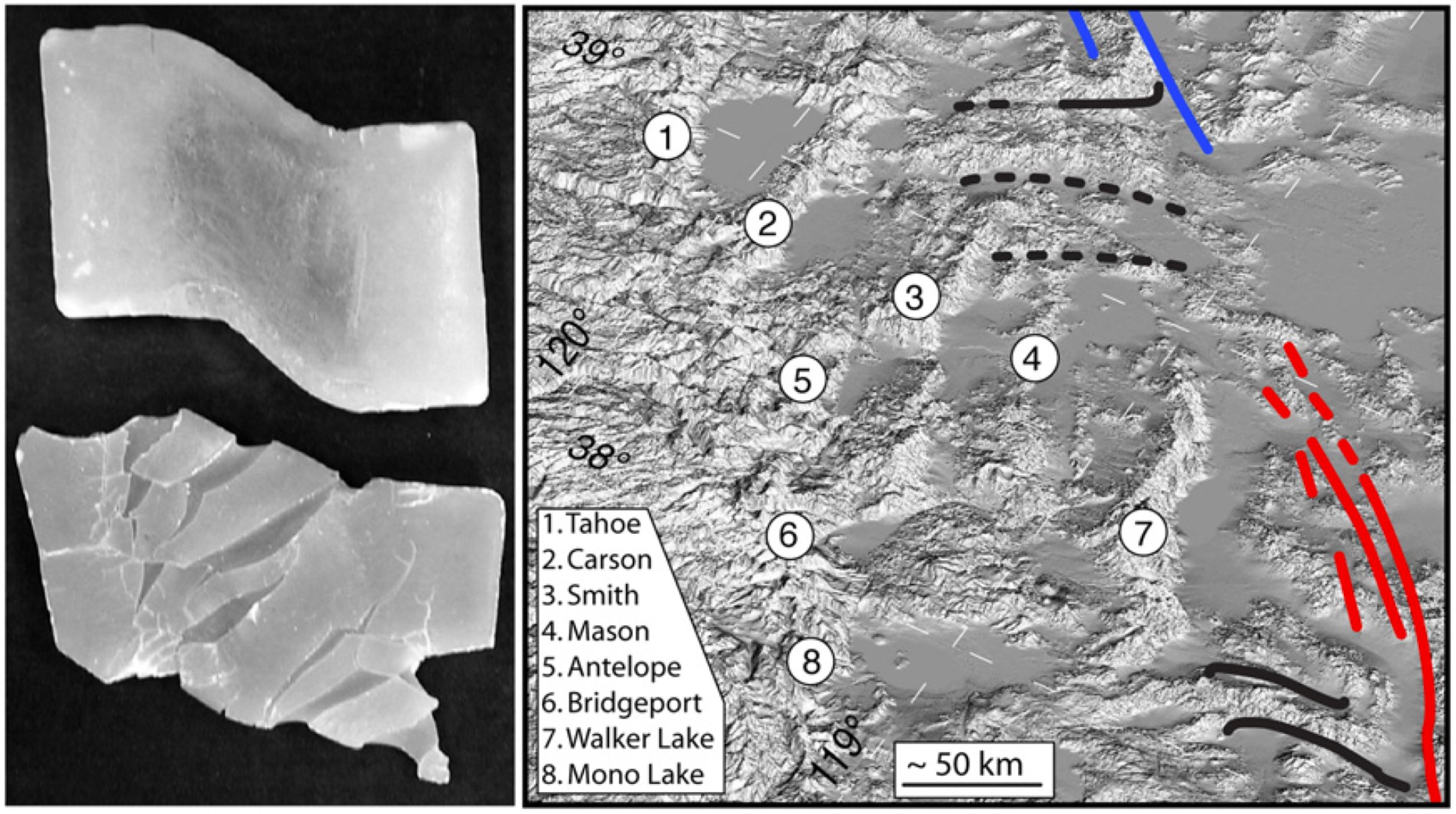
(Left) Model to visualize accommodation of strain and development of basins in northern Walker lane. The upper is a block of wax has been heated to become ductile and subjected to transtensional right-lateral shear. Ice has been applied to the surface of lower wax block to create brittle upon ductile layer, and then subjected to same shear. The transtensional shear results in a zone of deformation displaying rotation of ‘crustal blocks’, an en echelon arrangement of asymmetric ‘basins,’ observable extension along the axis of shear, and the ability to locally traverse the entire zone of shear without encountering a major fault structure. (Right) Oblique view of study area illustrates the en echelon arrangement and triangular shape of basins nested along the east edge of the Sierra Nevada. Black and colored lines are portions of Walker Lane faults shown in Fig. 1 (Wesnousky et al., 2012)
- Here are the geodetic observations for each of these blocks along the Walker Lane (Wesnousky et al., 2012). GPS rates are plotted as red vectors. Geologic rates are in the white boxes and are plotted as vectors in black, purple, and blue. Today’s earthquake series happened in the basin where the label “LUCK” is. Note how the GPS site on the northeast side of the basin is moving slightly faster than the GPS site on the western side of the basin. A northwesterly striking right-lateral strike-slip fault could produce this if it ran between these two GPS sites.
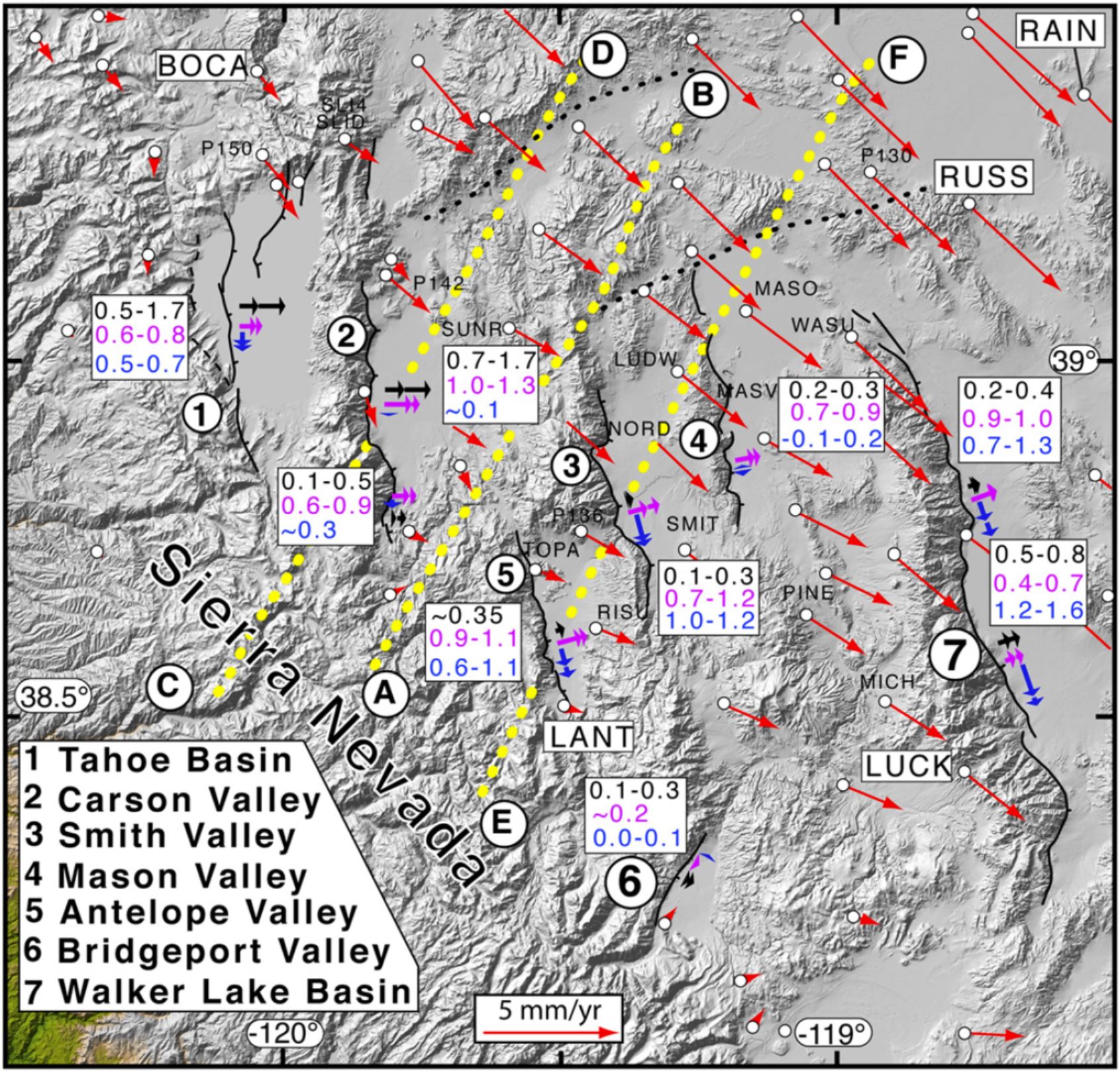
Physiographic and fault map of area of interest in northern Walker Lane shows major structural basins (numbered), active basin-bounding faults (thick black lines), and geodetic displacement field (red arrows). Shown in white boxes are geologically determined values of fault-normal extension (black-upper text), geodetic estimates of fault-normal extension (magenta-middle text) and geodetic estimates of fault-parallel strike-slip (blue-lower text) rates along each of the basin bounding faults. Two-headed arrows schematically show ranges of same values and correspond in arrangement and color to the values in boxes. The geologically determined extension rate arrows are placed adjacent to the sites of studies except for Lake Tahoe where the estimate is an average value across several submarine faults. Dotted (yellow) lines define paths AB, CD, and EF.
- This is the tectonic domain figure from Bormann et al. (2016). Some faults have arrows that show their relative sense of motion and blocks have arrows that show their relative sense of rotation. Note the east-west sinistral strike-slip faults that bound the northern and southern boundaries of the blocks in the Mina deflection. Today’s earthquakes happened along the eastern boundary of the Bodie Hills tectonic domain (BH). The BH domain has clockwise rotation like in the Mina deflection. This would place sinistral strain along the southern boundary of the BH domain, creating left-lateral strike-slip faults oriented northeast striking. This is consistent with the sense of motion along the “unnamed faults near Alkali Valley.” If these 2016 earthquakes are associated with these faults, then they are along northeast striking structures and would be left-lateral.
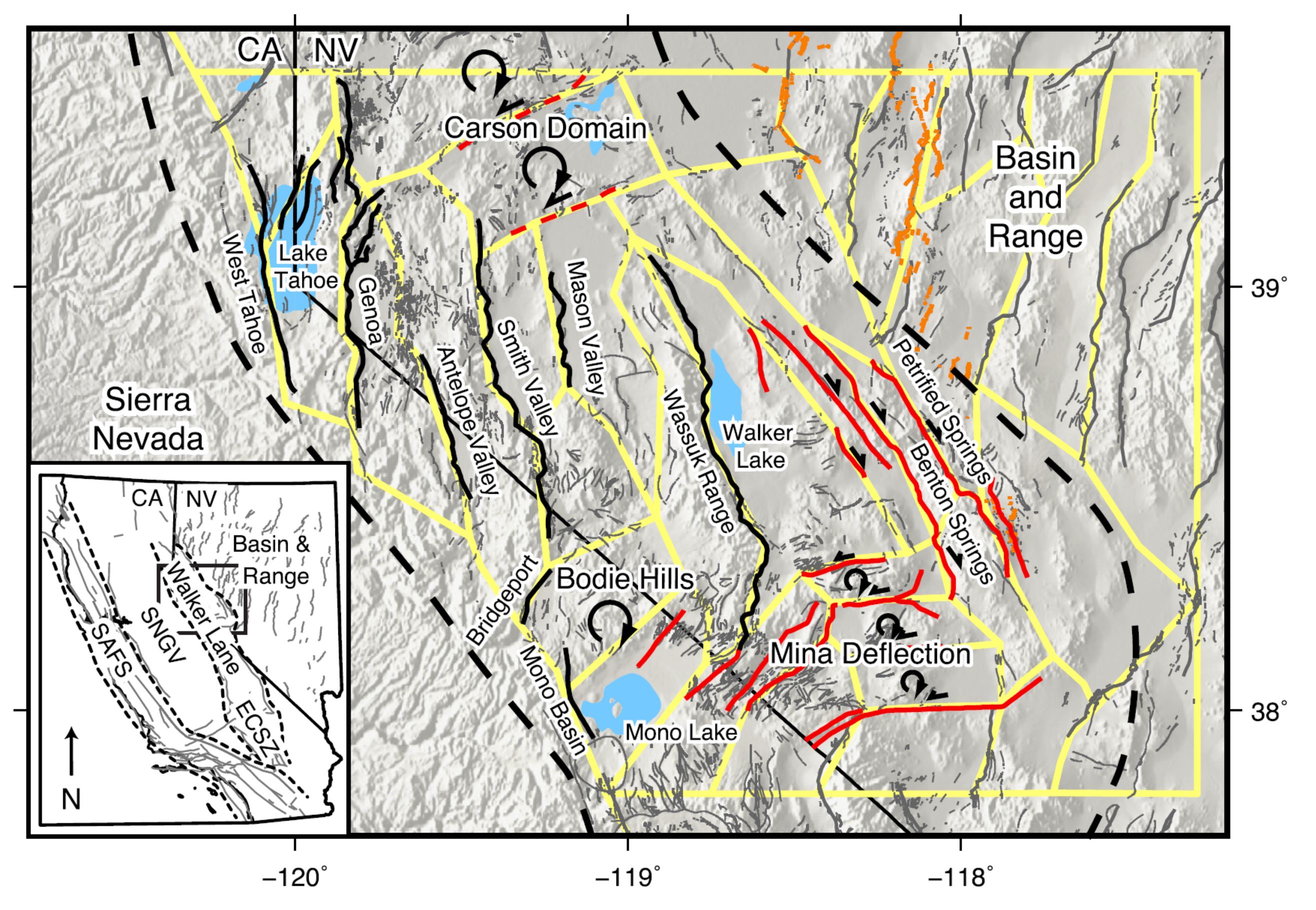
Regional map showing the block model boundaries (yellow lines) in relation to the topography and faults of the Central Walker Lane. The Central Walker Lane (region within the dashed black lines) lies between the northeast striking normal faults of the Basin and Range and the Sierra Nevada microplate. Black lines delin-eate major normal faults of the Central Walker Lane, and red lines mark the location of strike slip faults (arrows indicate slip direction). Paleomagnetic observations in-dicate that crustal blocks in the Carson Domain, Bodie Hills, and Mina Deflection accommodate dextral shear through clockwise vertical axis rotations (Cashman and Fontaine, 2000; Petronis et al., 2009; Rood et al., 2011b; Carlson et al., 2013). Orange lines mark the locations of surface rupture that resulted from historic earthquakes in the Central Nevada Seismic Belt. Faults traces are modified from the USGS Qua-ternary Fault and Fold database (U.S. Geological Survey, California Geological Survey, Nevada Bureau of Mines and Geology, 2006). Inset map shows the location of the study area in relation to other elements of the Pacific/North America Plate boundary zone.
- Here Bormann et al. (2016) present their estimates of rotation and fault slip rates for this region. The caption is below the figure. I place a red star where today’s earthquakes happened. This map helps us visualize an alternate interpretation of these earthquakes. The 2016 swarm is along the eastern boundary of the BH domain, which would suggest a northwest striking dextral (right-lateral) strike slip fault would be involved. Given that the currently mapped faults in this region are northeast striking, I interpret these to be along structures that are also northeast striking. Note how the BH domain is rotating clockwise about 1.75 °/Ma, while the MD is rotating clockwise about 2.75 °/Ma.
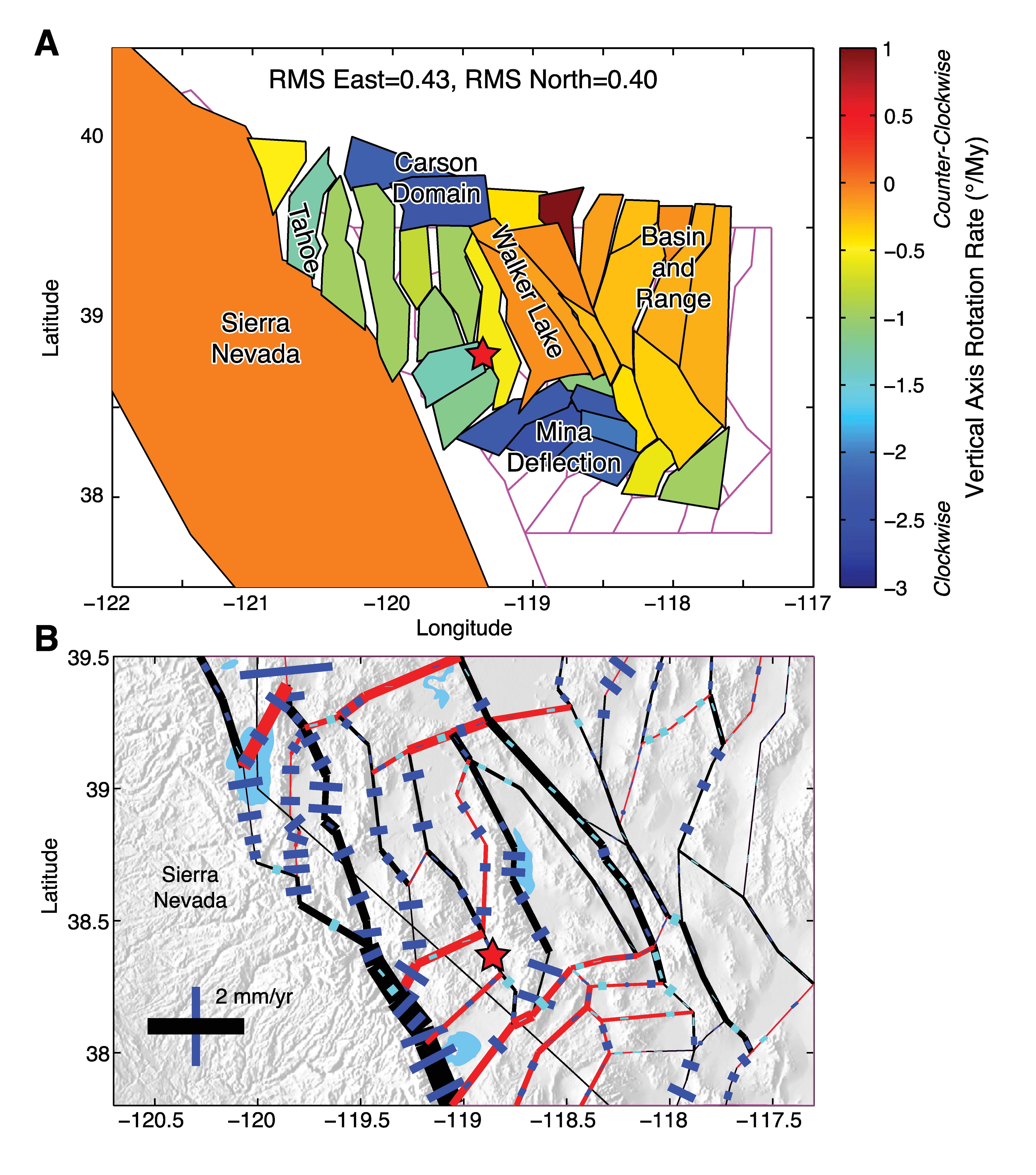
Block motions, slip rates, and velocity residuals for the best fitting GPS model. (A) Rigid block rotation and translation exaggerated by a factor of 107(representing 10 million years of deformation). Color of block indicates vertical axis rotation rate. (B) Predicted fault slip rates represented by the thickness of black (red) line for dextral (sinistral) strike-slip motion and the length of blue (cyan) bar for fault normal extension (compression).
- Here is the illustrative model presented by Lee et al. (2009) to explain the faulting in the MD (which may also partially explain the seismicity in this region northeast of the Bodie Hills).
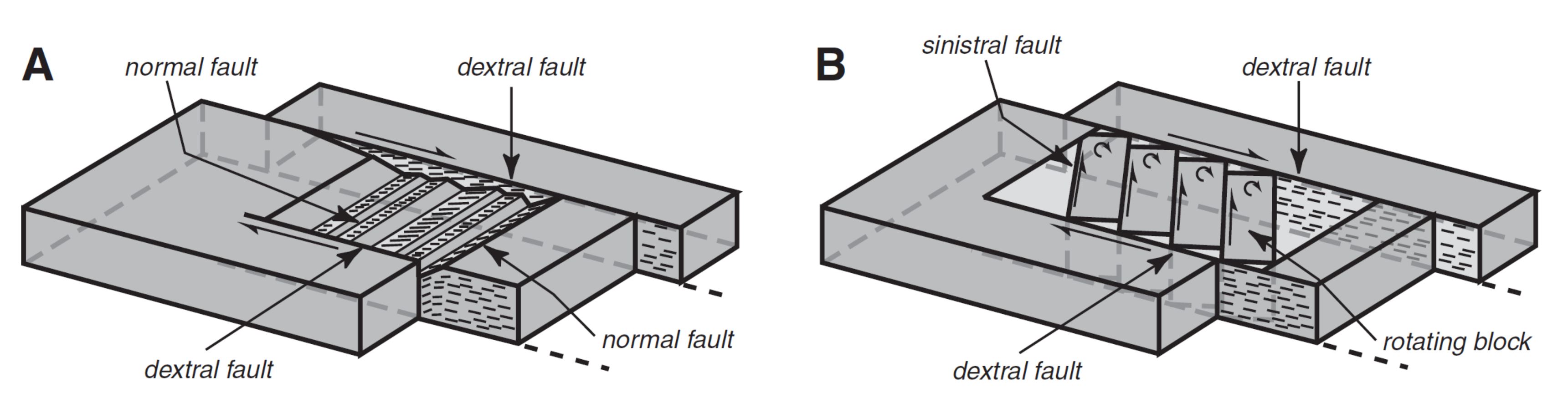
Schematic block diagrams illustrating two fault-slip transfer mechanisms between subparallel strike-slip faults proposed for the eastern California shear zone and Walker Lane belt. (A) Displacement transfer model whereby the magnitude of extension along the connecting normal faults is proportional to the amount of strike-slip motion transferred (modified from Oldow et al., 1994). (B) Block rotation model in which clockwise rotation of blocks, bounded by dextral faults, is accommodated by sinistral faults (model of McKenzie and Jackson, 1983, 1986).
- Here is an updated figure to show how these fault systems may have evolved through time (Nagorsen-Rinke et al., 2012).
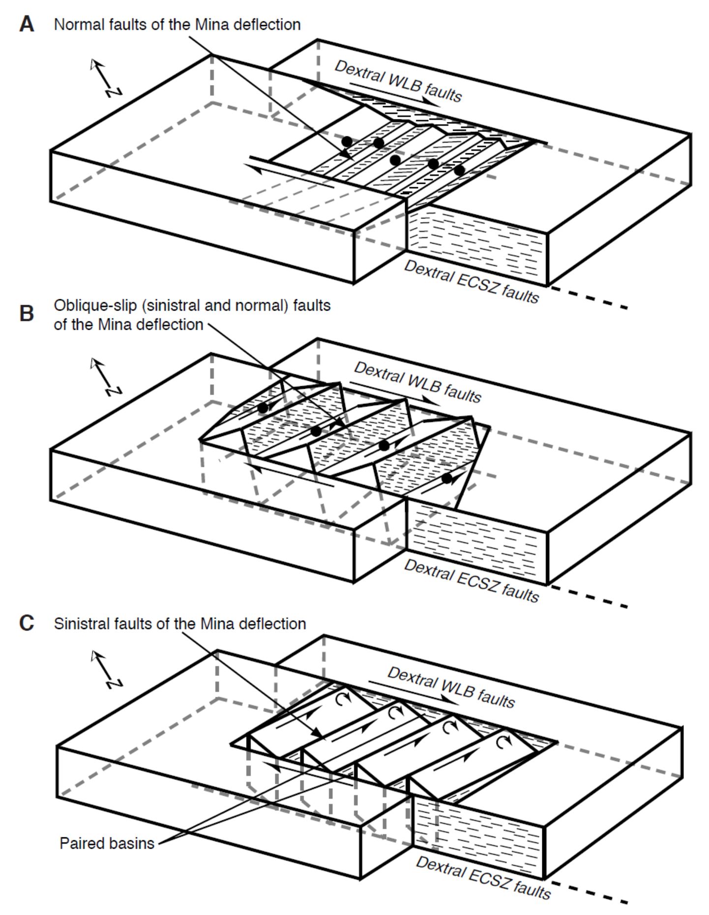
Block diagrams illustrating models proposed to explain fault slip transfer across the Mina deflection. (A) Displacement transfer model in which normal slip along connecting faults transfers fault slip (modified from Oldow, 1992; Oldow et al., 1994). (B) Transtensional model showing a combination of sinistral and normal slip along connecting faults. (C) Clockwise block rotation model in which sinistral slip along connecting faults, combined with vertical axis rotation of intervening fault blocks, transfers fault slip (modified from McKenzie and Jackson, 1983, 1986). Single-barbed arrows show dextral fault motion across faults of the Eastern California shear zone (ECSZ) and Walker Lane belt (WLB) and sinistral motion along faults in the Mina deflection; half-circle double-barbed arrows indicate clockwise rotating fault blocks; solid ball is located on the hanging wall of normal slip faults; thin short lines indicate slip direction on fault surfaces.
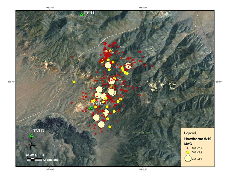
- Here is the map from the UNR Seismological Laboratory website. This shows the earthquakes recorded during the 2011 swarm along the “unnamed faults along Alakali Valley.” Here is the UNRSL website for this earthquake. I include the UNRSL description of the 2011 Hawthorne Sequence below.
- Over the past nine weeks 42 earthquakes of Magnitude 3.0 and larger earthquakes (listed below) have been located in a sequence about 12 miles southwest of Hawthorne, Nevada. The first of these occurred on March 15th at 11:14 AM PDT and the latest at 10:23 AM PDT on May 19th. The preliminary magnitude for the largest event is M 4.6.
- In all, there have been several hundred events of Magnitude 1 and larger; only a small fraction of the entire sequence has been reviewed. There have been 1000’s of smaller magnitude events.
- The Nevada Seismological Laboratory deployed 3 temporary telemetered instruments in the source area on April 17-19 including a NetQuakes instrument at the Court House in Hawthorne. These temporary telemetered instruments deliver real-time data to the data center in Reno and are configured with 3-channel broadband sensors and 3-channel accelerometers.
- Here is a map from Nagorsen-Rinke et al. (2012) with regional faults mapped. Note how the sinistral faults that bound blocks in the Mina deflection are each slightly more counterclockwise rotated with the fault at the base of the southeastern Excelsior Mountains being the most northerly striking of these faults. If this configuration of faulting were in the basin to the NE of the Bodie Hills, it would explain the northeast striking sinistral interpretation for the 2016 series.
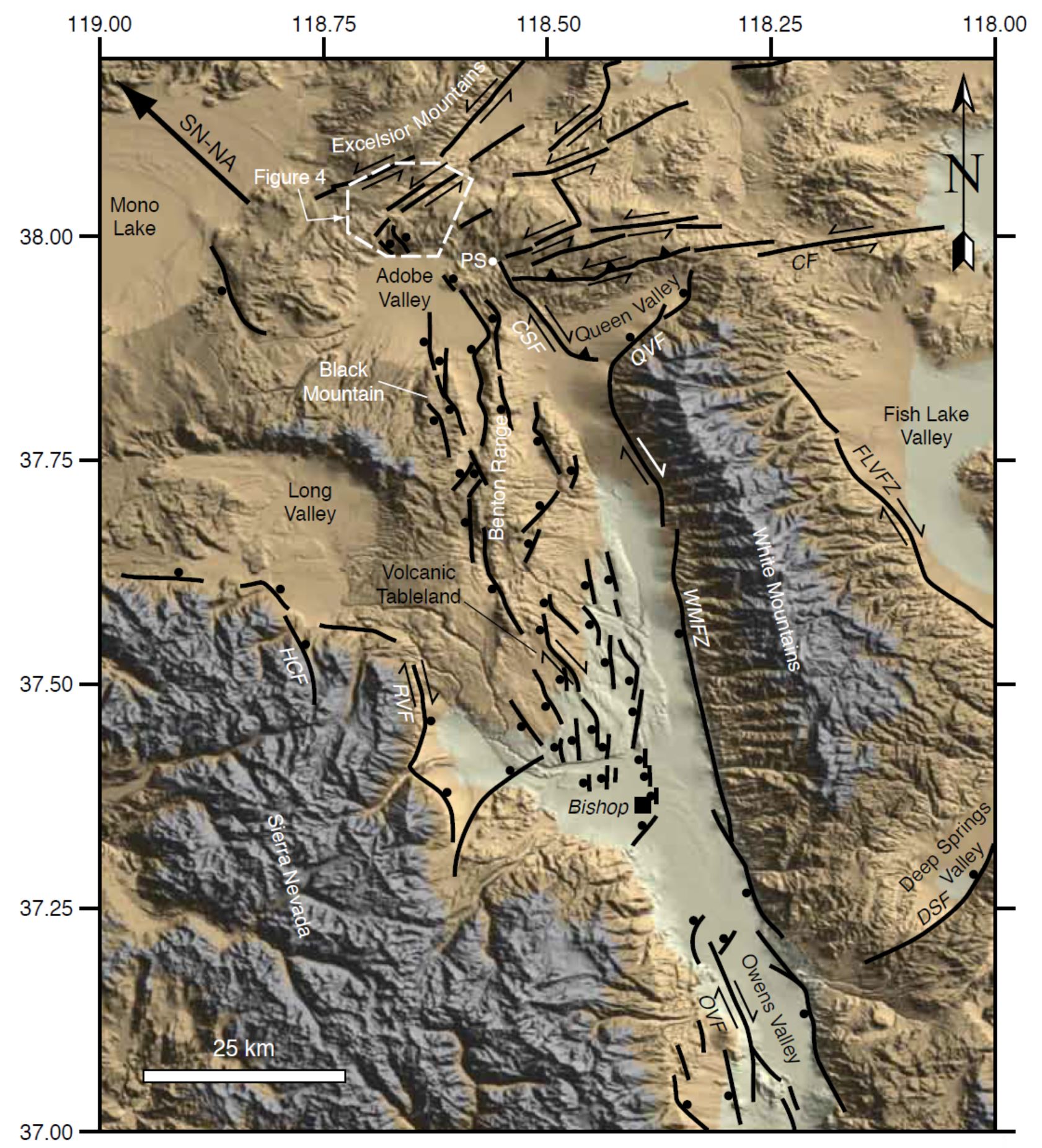
Shaded relief map of the southern part of the Mina deflection and northern part of the eastern California shear zone showing the major Quaternary faults. Solid black ball is located on the hanging wall of normal faults; arrow pairs indicate relative motion across strike-slip faults. Heavy arrow in northwest corner of map shows the present-day motion of the Sierra Nevada (SN) with respect to North America (NA) (Dixon et al., 2000). Location of the Adobe Hills geologic map shown in Figure 4A is outlined with a dashed line and location of this map is shown in Figure 1. PS—Pizona Springs; CF—Coaldale fault; CSF— Coyote Springs fault; DSF—Deep Springs fault; FLVFZ—Fish Lake Valley fault zone; HCF—Hilton Creek fault; OVF—Owens Valley fault; QVF—Queen Valley fault; RVF— Round Valley fault; WMFZ—White Mountains fault zone.
- 2020.03.18 M 5.7 Salt Lake City, Utah
- 2020.03.31 M 6.5 Idaho
- 2017.09.02 M 5.3 Idaho
- 2020.05.15 M 6.5 Nevada
- 2016.12.28 M 5.7 swarm Nevada
- 2014.11.05 M 4.6 swarm Nevada
- Frisch, W., Meschede, M., Blakey, R., 2011. Plate Tectonics, Springer-Verlag, London, 213 pp.
- Hayes, G., 2018, Slab2 – A Comprehensive Subduction Zone Geometry Model: U.S. Geological Survey data release, https://doi.org/10.5066/F7PV6JNV.
- Holt, W. E., C. Kreemer, A. J. Haines, L. Estey, C. Meertens, G. Blewitt, and D. Lavallee (2005), Project helps constrain continental dynamics and seismic hazards, Eos Trans. AGU, 86(41), 383–387, , https://doi.org/10.1029/2005EO410002. /li>
- Jessee, M.A.N., Hamburger, M. W., Allstadt, K., Wald, D. J., Robeson, S. M., Tanyas, H., et al. (2018). A global empirical model for near-real-time assessment of seismically induced landslides. Journal of Geophysical Research: Earth Surface, 123, 1835–1859. https://doi.org/10.1029/2017JF004494
- Kreemer, C., J. Haines, W. Holt, G. Blewitt, and D. Lavallee (2000), On the determination of a global strain rate model, Geophys. J. Int., 52(10), 765–770.
- Kreemer, C., W. E. Holt, and A. J. Haines (2003), An integrated global model of present-day plate motions and plate boundary deformation, Geophys. J. Int., 154(1), 8–34, , https://doi.org/10.1046/j.1365-246X.2003.01917.x.
- Kreemer, C., G. Blewitt, E.C. Klein, 2014. A geodetic plate motion and Global Strain Rate Model in Geochemistry, Geophysics, Geosystems, v. 15, p. 3849-3889, https://doi.org/10.1002/2014GC005407.
- Meyer, B., Saltus, R., Chulliat, a., 2017. EMAG2: Earth Magnetic Anomaly Grid (2-arc-minute resolution) Version 3. National Centers for Environmental Information, NOAA. Model. https://doi.org/10.7289/V5H70CVX
- Müller, R.D., Sdrolias, M., Gaina, C. and Roest, W.R., 2008, Age spreading rates and spreading asymmetry of the world’s ocean crust in Geochemistry, Geophysics, Geosystems, 9, Q04006, https://doi.org/10.1029/2007GC001743
- Pagani,M. , J. Garcia-Pelaez, R. Gee, K. Johnson, V. Poggi, R. Styron, G. Weatherill, M. Simionato, D. Viganò, L. Danciu, D. Monelli (2018). Global Earthquake Model (GEM) Seismic Hazard Map (version 2018.1 – December 2018), DOI: 10.13117/GEM-GLOBAL-SEISMIC-HAZARD-MAP-2018.1
- Silva, V ., D Amo-Oduro, A Calderon, J Dabbeek, V Despotaki, L Martins, A Rao, M Simionato, D Viganò, C Yepes, A Acevedo, N Horspool, H Crowley, K Jaiswal, M Journeay, M Pittore, 2018. Global Earthquake Model (GEM) Seismic Risk Map (version 2018.1). https://doi.org/10.13117/GEM-GLOBAL-SEISMIC-RISK-MAP-2018.1
- Zhu, J., Baise, L. G., Thompson, E. M., 2017, An Updated Geospatial Liquefaction Model for Global Application, Bulletin of the Seismological Society of America, 107, p 1365-1385, https://doi.org/0.1785/0120160198
- Sorted by Magnitude
- Sorted by Year
- Sorted by Day of the Year
- Sorted By Region
Basin and Range
General Overview
Earthquake Reports
Utah
Idaho
Nevada
Social Media
First-motion mechanism: Mw6.4 #earthquake California – Nevada Border Region
Shows strike-slip faulting https://t.co/6dsdgupJzY pic.twitter.com/zMm4VSdVTM— Anthony Lomax 🌍🇪🇺 (@ALomaxNet) May 15, 2020
Mw=6.5, NEVADA (Depth: 10 km), 2020/05/15 11:03:26 UTC – Full details here: https://t.co/Q4iICPhE1H pic.twitter.com/ZpxNMOu8gO
— Earthquakes (@geoscope_ipgp) May 15, 2020
#earthquake This mornings earthquake outside Tonopah has damaged a portion of US95 at Mile Marker 98 in Esmerelda County. US 95 is closed in both directions, seek alternate routes. DOT is on scene making repairs, no timeframe given. #nhpsocomm pic.twitter.com/IF2Dp1s3Zc
— NHP Southern Command (@NHPSouthernComm) May 15, 2020
GSN and other global surface & body wave record sections for the Mww 6.5 NEVADA https://t.co/ek0b6iw69i pic.twitter.com/6HmqiEzlC0
— IRIS Earthquake Sci (@IRIS_EPO) May 15, 2020
Aftershocks from the M6.5 #NevadaEarthquake cluster in proximity to the mainshock, as expected but, interestingly, the sequence includes a halo of more distance aftershocks… pic.twitter.com/UnAImI9j30
— Susan Hough (@SeismoSue) May 15, 2020
.@EsmeraldaCounty Sheriff showing the damage down after the 6.5 magnitude earthquake near Mina, NV.
Road damage and hazards on Hwy 95 and US 6 this morning. pic.twitter.com/K998rhVOvK
— Steve Bender (@SteveBenderWx) May 15, 2020
Watch the waves from the M6.5 #NevadaEarthquake roll across seismic stations in North America! (THREAD) pic.twitter.com/4SHwiMWtRK
— IRIS Earthquake Sci (@IRIS_EPO) May 15, 2020
Eyewitnesses are RT sensors of M6.4 Nevada quake! Look at the propagation of the propagation of seismic waves and how fast users launch LastQuake app (orange dots) pic.twitter.com/9QAi5GBJ2k
— EMSC (@LastQuake) May 15, 2020
Auto solution FMNEAR (Géoazur/OCA) with regional records for the 2020/05/15 11:03:28 M6.5 NEVADA, USA(Loc EMSC used to trigger inversion).https://t.co/UHDsc1hVXA (not on mobile version)
Thanks to the seismic records provided by NCEDC, SCEC, and IRIS pic.twitter.com/LKGvEIRUtK— Bertrand Delouis (@BertrandDelouis) May 15, 2020
Real-time displacements for the Tonopah EQ this morning at P132. This site is roughly 65 km north of the event, so the signal is transverse to the propagation direction. @UNAVCO pic.twitter.com/CkdmhOV9uy
— Brendan Crowell (@bwcphd) May 15, 2020
Aftershocks to Mina/Tonopah M6.5 #earthquake as of about 1800hrs. Definitely looks like sinistral E-W plane, which would fit with possible surface rupture on US95 pic.twitter.com/xdsyvFaVPR
— Michael Bunds (@cataclasite) May 15, 2020
And some velocities at P133, 81 km north of the Tonopah EQ. Similar strong east motions, would be roughly MMI4. pic.twitter.com/hVzZlp84YR
— Brendan Crowell (@bwcphd) May 15, 2020
Auto slipmap with regional records (SLIPNEAR method, single fault plane) for the 2020/05/15 11:03:28 M6.5 NEVADA(Loc EMSC), FM solution FMNEAR. Plane NS (strike 355) selected as rupt plane, possible directivity towards the North.
Géoazur/OCA – EU project SERA pic.twitter.com/mTXgrDFZJL
— Bertrand Delouis (@BertrandDelouis) May 15, 2020
Interesting! Looks like similar strong E-W displacements at Little Huntoon Valley station (56 km west of epicenter). Almost 2 cm, not too shabby. pic.twitter.com/JItG0H8Kl0
— Brian OLSON-19 (@mrbrianolson) May 15, 2020
Strong Nevada earthquake felt in San Francisco Bay Area, Bakersfield a https://t.co/xWjXtgo1Nl via @temblor
— temblor (@temblor) May 15, 2020
Finally, it's worth noting how today's sequence sits with respect to a line of ruptures extending from 2019 Ridgecrest to 1915 Pleasant Valley. Does this portend anything larger? Dunno, there are so many active faults in here you can almost choose your own adventure. But: Yikes. pic.twitter.com/Go7fzQlMMW
— Rich Briggs (@rangefront) May 16, 2020
@patton_cascadia The stress modeling caused by the Mw 6.4 on optimally oriented strike slip faults show a causative relation between stress and aftershocks distributions. The regional stress used in this second modeling are from Frizzell and Zoback ( https://t.co/ueLHOWVihn) pic.twitter.com/BwEO83QmgP
— Jugurtha Kariche (@JkaricheKariche) May 16, 2020
Final tweet of this thread (my first thread!) – circling back to #MinaDeflection! Here are source focal mechs aka beach balls for ~330 #earthquakes and a preliminary stress inversion I did 6 years ago as part of my #dissertation #proposal Green=LL, Yellow=RL, Red=Normal pic.twitter.com/qgdlpIaqHx
— Dr. Christine J. Ruhl (@christineruhl) May 16, 2020
It also might be "ground oscillation" as described by Youd (1995). This is common on very flat ground surfaces (<<2%). When you saw it on the ground, did you observe any sand boils along the margins or within the disturbed ground? pic.twitter.com/Xas2qnmHsv
— Brian OLSON-19 (@mrbrianolson) May 16, 2020
UPDATE 2020.06.11
— Cynthia L. Pridmore (@earthquakemom) June 11, 2020
References:
Basic & General References
Specific References
Return to the Earthquake Reports page.