Earthquake Report: Loyalty Islands

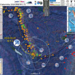
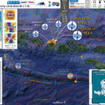
The earthquakes continue, every day. Today, there was a large earthquake along the southern New Hebrides Trench.

Today’s M 7.1 earthquake happened along one of the more active subduction zones in the world.

The hypocentral (3-D location) depth of ~26 km is very close to the depth where we think the subduction zone megathrust fault may be. So, it is possible that this M 7.1 earthquake ruptured the megathrust. Though, it is also possible that this represents slip on a subsidiary fault (e.g. in the upper plate).

In November 2017 there was an earthquake that helped us learn about this region (just like today’s earthquake).

There have been some tsunami waves recorded. Here are the measurements from the National Weather Service, Pacific Tsunami Warning Center in Hawai’i. Below are also additional announcements. More can be found at tsunami.gov.


Below is my interpretive poster for this earthquake

I plot the seismicity from the past month, with color representing depth and diameter representing magnitude (see legend). I include earthquake epicenters from 1918-2018 with magnitudes M ≥ 7.0 in one version.

I plot the USGS fault plane solutions (moment tensors in blue and focal mechanisms in orange), possibly in addition to some relevant historic earthquakes.

  • I placed a moment tensor / focal mechanism legend on the poster. There is more material from the USGS web sites about moment tensors and focal mechanisms (the beach ball symbols). Both moment tensors and focal mechanisms are solutions to seismologic data that reveal two possible interpretations for fault orientation and sense of motion. One must use other information, like the regional tectonics, to interpret which of the two possibilities is more likely.
  • I also include the shaking intensity contours on the map. These use the Modified Mercalli Intensity Scale (MMI; see the legend on the map). This is based upon a computer model estimate of ground motions, different from the “Did You Feel It?” estimate of ground motions that is actually based on real observations. The MMI is a qualitative measure of shaking intensity. More on the MMI scale can be found here and here. This is based upon a computer model estimate of ground motions, different from the “Did You Feel It?” estimate of ground motions that is actually based on real observations.
  • I include the slab contours plotted (Hayes et al., 2012), which are contours that represent the depth to the subduction zone fault. These are mostly based upon seismicity. The depths of the earthquakes have considerable error and do not all occur along the subduction zone faults, so these slab contours are simply the best estimate for the location of the fault.

    Magnetic Anomalies

  • In the map below, I include a transparent overlay of the magnetic anomaly data from EMAG2 (Meyer et al., 2017). As oceanic crust is formed, it inherits the magnetic field at the time. At different points through time, the magnetic polarity (north vs. south) flips, the north pole becomes the south pole. These changes in polarity can be seen when measuring the magnetic field above oceanic plates. This is one of the fundamental evidences for plate spreading at oceanic spreading ridges (like the Gorda rise).
  • Regions with magnetic fields aligned like today’s magnetic polarity are colored red in the EMAG2 data, while reversed polarity regions are colored blue. Regions of intermediate magnetic field are colored light purple.

    I include some inset figures. Some of the same figures are located in different places on the larger scale map below.

  • In the upper left corner I include the map and seismicity cross section from Benz et al. (2011). These maps plot the seismicity and this reveals the nature of the downgoing subducting slab. Shallower earthquakes are generally more related to the subduction zone fault or deformation within either plate (interplate and intraplate earthquakes). While the deeper earthquakes are not megathrust fault related, but solely due to internal crustal deformation (intraplate earthquakes). I highlight the location of the cross section with a blue line labeled F-F’ and G-G’.
  • In the lower left corner are the cross sections F-F’ and G-G’. These figures use seismicity to show how the subduction zone dips to the east.
  • In the upper right corner is a figure from Richards et al. (2011). This is a map that shows the location of downgoing slabs (chunks of oceanic lithosphere), in red, that the authors have interpreted.
  • In the lower right corner is a series of illustrations showing the Richards et al. (2011) interpretation of the evolution of the slabs related to the New Hebrides subduction zone.
  • Here is the map with a month’s seismicity plotted.

  • Here is the map with a centuries seismicity plotted.

  • The 2 posters below review the earthquakes from November 2017.

  • Here is my poster from the beginning of this sequence.

Other Report Pages

Some Relevant Discussion and Figures

  • Here is a map from the USGS report (Benz et al., 2011). Read more about this map on the USGS website. Earthquakes are plotted with color related to depth and circle diameter related to magnitude. Today’s M 6.8 earthquake occurred south of cross section G-G’.

  • This is the legend.

  • Here is a cross section showing the seismicity along swatch profile G-G’.


  • Craig et al. (2014) evaluated the historic record of seismicity for subduction zones globally. In particular, the evaluated the relations between upper and lower plate stresses and earthquake types (cogent for the southern New Hebrides trench). Below is a figure from their paper for this part of the world. I include their figure caption below in blockquote.

  • Outer-rise seismicity along the New Hebrides arc. (a) Seismicity and focal mechanisms. Seismicity at the southern end of the arc is dominated by two major outer-rise normal faulting events, and MW 7.6 on 1995 May 16 and an MW 7.1 on 2004 January 3. Earthquakes are included from Chapple & Forsyth (1979); Chinn & Isacks (1983); Liu & McNally (1993). (b) Time versus latitude plot.

  • Here is a summary figure from Craig et al. (2014) that shows different stress configurations possibly existing along subduction zones.

  • Schematic diagram for the factors influencing the depth of the transition from horizontal extension to horizontal compression beneath the outer rise. Slab pull, the interaction of the descending slab with the 660 km discontinuity (or increasing drag from the surround mantle), and variations in the interface stress influence both the bending moment and the in-plane stress. Increases in the angle of slab dip increases the dominance of the bending moment relative to the in-plane stress, and hence moves the depth of transition towards the middle of the mechanical plate from either an shallower or a deeper position. A decrease in slab dip enhances the influence of the in-plane stress, and hence moves the transition further from the middle of the mechanical plate, either deeper for an extensional in-plane stress, or shallower for a compressional in-plane stress. Increased plate age of the incoming plate leads to increases in the magnitude of ridge push and intraplate thermal contraction, increasing the in-plane compressional stress in the plate prior to bending. Dynamic topography of the oceanic plate seawards of the trench can result in either in-plane extension or compression prior to the application of the bending stresses.

  • Here is a great figure from here, the New Caledonian Seismologic Network. This shows how geologists have recorded uplift rates along dip (“perpendicular” to the subduction zone fault). On the left is a map and on the right is a vertical profile showing how these rates of uplift change east-west. This is the upwards flexure related to the outer rise, which causes extension in the upper part of the downgoing/subducting plate.

  • The subduction of the Australian plate under the Vanuatu arc is also accompanied by vertical movements of the lithosphere. Thus, the altitudes recorded by GPS at the level of the Quaternary reef formations that cover the Loyalty Islands (Ouvéa altitude: 46 m, Lifou: 104 m and Maré 138 m) indicate that the Loyalty Islands accompany a bulge of the Australian plate. just before his subduction. Coral reefs that have “recorded” the high historical levels of the sea serve as a reference marker for geologists who map areas in uprising or vertical depression (called uplift and subsidence). Thus, the various studies have shown that the Loyalty Islands, the Isle of Pines but alsothe south of Grande Terre (Yaté region) rise at speeds between 1.2 and 2.5 millimeters per decade.

  • Here are the figures from Richards et al. (2011) with their figure captions below in blockquote.
  • The main tectonic map

  • bathymetry, and major tectonic element map of the study area. The Tonga and Vanuatu subduction systems are shown together with the locations of earthquake epicenters discussed herein. Earthquakes between 0 and 70 km depth have been removed for clarity. Remaining earthquakes are color-coded according to depth. Earthquakes located at 500–650 km depth beneath the North Fiji Basin are also shown. Plate motions for Vanuatu are from the U.S. Geological Survey, and for Tonga from Beavan et al. (2002) (see text for details). Dashed line indicates location of cross section shown in Figure 3. NFB—North Fiji Basin; HFZ—Hunter Fracture Zone.

  • Here is the map showing the current configuration of the slabs in the region.

  • Map showing distribution of slab segments beneath the Tonga-Vanuatu region. West-dipping Pacifi c slab is shown in gray; northeast-dipping Australian slab is shown in red. Three detached segments of Australian slab lie below the North Fiji Basin (NFB). HFZ—Hunter Fracture Zone. Contour interval is 100 km. Detached segments of Australian plate form sub-horizontal sheets located at ~600 km depth. White dashed line shows outline of the subducted slab fragments when reconstructed from 660 km depth to the surface. When all subducted components are brought to the surface, the geometry closely approximates that of the North Fiji Basin.

  • This is the cross section showing the megathrust fault configuration based on seismic tomography and seismicity.

  • Previous interpretation of combined P-wave tomography and seismicity from van der Hilst (1995). Earthquake hypocenters are shown in blue. The previous interpretation of slab structure is contained within the black dashed lines. Solid red lines mark the surface of the Pacifi c slab (1), the still attached subducting Australian slab (2a), and the detached segment of the Australian plate (2b). UM—upper mantle;
    TZ—transition zone; LM—lower mantle.

  • Here is their time step interpretation of the slabs that resulted in the second figure above.

  • Simplified plate tectonic reconstruction showing the progressive geometric evolution of the Vanuatu and Tonga subduction systems in plan view and in cross section. Initiation of the Vanuatu subduction system begins by 10 Ma. Initial detachment of the basal part of the Australian slab begins at ca. 5–4 Ma and then sinking and collision between the detached segment and the Pacifi c slab occur by 3–4 Ma. Initial opening of the Lau backarc also occurred at this time. Between 3 Ma and the present, both slabs have been sinking progressively to their current position. VT—Vitiaz trench; dER—d’Entrecasteaux Ridge.

  • Here is an animation that shows the seismicity for this region from 1960 – 2016 for earthquakes with magnitudes greater than or equal to 7.0.
  • I include some figures mentioned in my report from 2016.04.28 for a sequence of earthquakes in the same region as today’s earthquake (albeit shallower hypocentral depths), in addition to a plot from Cleveland et al. (2014). In the upper right corner, Cleveland et al. (2014) on the left plot a map showing earthquake epicenters for the time period listed below the plot on the right. On the right is a plot of earthquakes (diameter = magnitude) of earthquakes with latitude on the vertical axis and time on the horizontal axis. Cleveland et al (2014) discuss these short periods of seismicity that span a certain range of fault length along the New Hebrides Trench in this area. Above is a screen shot image and below is the video.

  • Here is a link to the embedded video below (6 MB mp4)
    Here are the two figures from Cleveland et al. (2014).

  • Figure 1. I include the figure caption below as a blockquote.

  • (left) Seismicity of the northern Vanuatu subduction zone, displaying all USGS-NEIC earthquake hypocenters since 1973. The Australian plate subducts beneath the Pacific in nearly trench-orthogonal convergence along the Vanuatu subduction zone. The largest events are displayed with dotted outlines of the magnitude-scaled circle. Convergence rates are calculated using the MORVEL model for Australia Plate relative to Pacific Plate [DeMets et al., 2010]. (right) All GCMT moment tensor solutions and centroids for Mw ≥ 5 since 1976, scaled with moment. This region experiences abundant moderate and large earthquakes but lacks any events with Mw >8 since at least 1900.

  • Figure 17. I include the figure caption below as a blockquote.

  • One hundred day aftershock distributions of all earthquakes listed in the ISC catalog for the 1966 sequence and in the USGS-NEIC catalog for the 1980, 1997, 2009, and 2013 sequences in northern Vanuatu. The 1966 main shocks are plotted at locations listed by Tajima et al. [1990]. Events of the 1997 and 2009 sequences were relocated using the double difference method [Waldhauser and Ellsworth, 2000] for P wave first arrivals based on EDR picks. The event symbol areas are scaled relative to the earthquake magnitudes based on a method developed by Utsu and Seki [1954]. Hypocenters of most aftershock events occurred at <50 km depth.

  • Figure 17. I include the figure caption below as a blockquote.

  • (right) Space-time plot of shallow (≤ 70 km) seismicity M ≥ 5.0 in northern Vanuatu recorded in the NEIC catalog as a function of distance south of 10°N, 165.25°E. (left) The location of the seismicity on a map rotated to orient the trench vertically.

Geologic Fundamentals

  • For more on the graphical representation of moment tensors and focal mechnisms, check this IRIS video out:
  • Here is a fantastic infographic from Frisch et al. (2011). This figure shows some examples of earthquakes in different plate tectonic settings, and what their fault plane solutions are. There is a cross section showing these focal mechanisms for a thrust or reverse earthquake. The upper right corner includes my favorite figure of all time. This shows the first motion (up or down) for each of the four quadrants. This figure also shows how the amplitude of the seismic waves are greatest (generally) in the middle of the quadrant and decrease to zero at the nodal planes (the boundary of each quadrant).

  • Here is another way to look at these beach balls.
  • There are three types of earthquakes, strike-slip, compressional (reverse or thrust, depending upon the dip of the fault), and extensional (normal). Here is are some animations of these three types of earthquake faults. The following three animations are from IRIS.
  • Strike Slip:

    Compressional:

    Extensional:

  • This is an image from the USGS that shows how, when an oceanic plate moves over a hotspot, the volcanoes formed over the hotspot form a series of volcanoes that increase in age in the direction of plate motion. The presumption is that the hotspot is stable and stays in one location. Torsvik et al. (2017) use various methods to evaluate why this is a false presumption for the Hawaii Hotspot.

  • A cutaway view along the Hawaiian island chain showing the inferred mantle plume that has fed the Hawaiian hot spot on the overriding Pacific Plate. The geologic ages of the oldest volcano on each island (Ma = millions of years ago) are progressively older to the northwest, consistent with the hot spot model for the origin of the Hawaiian Ridge-Emperor Seamount Chain. (Modified from image of Joel E. Robinson, USGS, in “This Dynamic Planet” map of Simkin and others, 2006.)

  • Here is a map from Torsvik et al. (2017) that shows the age of volcanic rocks at different locations along the Hawaii-Emperor Seamount Chain.

  • Hawaiian-Emperor Chain. White dots are the locations of radiometrically dated seamounts, atolls and islands, based on compilations of Doubrovine et al. and O’Connor et al. Features encircled with larger white circles are discussed in the text and Fig. 2. Marine gravity anomaly map is from Sandwell and Smith.

    References:

  • Benz, H.M., Herman, M., Tarr, A.C., Hayes, G.P., Furlong, K.P., Villaseñor, A., Dart, R.L., and Rhea, S., 2011. Seismicity of the Earth 1900–2010 New Guinea and vicinity: U.S. Geological Survey Open-File Report 2010–1083-H, scale 1:8,000,000.
  • Bird, P., 2003. An updated digital model of plate boundaries in Geochemistry, Geophysics, Geosystems, v. 4, doi:10.1029/2001GC000252, 52 p.
  • Cleveland, K.M., Ammon, C.J., and Lay, T., 2014. Large earthquake processes in the northern Vanuatu subduction zone in Journal of Geophysical Research: Solid Earth, v. 119, p. 8866-8883, doi:10.1002/2014JB011289.
  • Craig, T.J., Copley, A., and Jackson, J., 2014. A reassessment of outer-rise seismicity and its implications for the mechanics of oceanic lithosphere in Geophysical Journal International, v. 197, p/ 63-89.
  • Geist, E.L., and Parsons, T., 2005, Triggering of tsunamigenic aftershocks from large strike-slip earthquakes: Analysis of the November 2000 New Ireland earthquake sequence: Geochemistry, Geophysics, Geosystems, v. 6, doi:10.1029/2005GC000935, 18 p. [Download PDF (6.5 MB)]
  • Hayes, G. P., D. J. Wald, and R. L. Johnson, 2012. Slab1.0: A three-dimensional model of global subduction zone geometries, J. Geophys. Res., 117, B01302, doi:10.1029/2011JB008524.
  • Lay, T., and Kanamori, H., 1980, Earthquake doublets in the Solomon Islands: Physics of the Earth and Planetary Interiors, v. 21, p. 283-304.
  • Lay, T., Ammon, C.J., Kanamori, H., Kim, M.J., and Xue, L., 2011. Outer trench-slope faulting and the 2011 Mw 9.0 off the Pacific coast of Tohoku Earthquake in Earth Planets Space,
    v. 63, p. 713-718.
  • Meyer, B., Saltus, R., Chulliat, a., 2017. EMAG2: Earth Magnetic Anomaly Grid (2-arc-minute resolution) Version 3. National Centers for Environmental Information, NOAA. Model. doi:10.7289/V5H70CVX
  • Richards, S., Holm, R., Barber, G., 2011. When slabs collide: A tectonic assessment of deep earthquakes in the Tonga-Vanuatu region in Geology, v. 39, no. 8., p. 787-790
  • Schwartz, S.Y., 1999, Noncharacteristic behavior and complex recurrence of large subduction zone earthquakes: Journal of Geophysical Research, v. 104, p. 23,111-123,125.
  • Schwartz, S.Y., Lay, T., and Ruff, L.J., 1989, Source process of the great 1971 Solomon Islands doublet: Physics of the Earth and Planetary Interiors, v. 56, p. 294-310.
    • Music Reference (in 19600-2016 seismicity video): Bumba Crossing Kevin MacLeod (incompetech.com) | Licensed under Creative Commons: By Attribution 3.0 License | http://creativecommons.org/licenses/by/3.0/

Return to the Earthquake Reports page.


°

ñ

Earthquake Report: Deep in Peru

Busy week!
Still
Got to this intermittently today and it is fine that it took me a while to get this report together. One might ask “why?”. Well, this earthquake, while having a large magnitude, was quite deep. Because earthquake intensity decreases with distance from the earthquake source, the shaking intensity from this earthquake was so low that nobody submitted a single report to the USGS “Did You Feel It?” website for this earthquake.
This report let me spend some time thinking about the historic earthquakes in this region. In other reports (e.g. the M 8.2 Fiji earthquake from a few days ago) I discuss various reasons why there are earthquakes at these great depths. I will mention some of that below, but in general, we think that there are various physical and chemical changes to earth materials at these great depths that lead to changes in stress and strain, leading to earthquakes.
While doing my lit review, I found the Okal and Bina (1994) paper where they use various methods to determine focal mechanisms for the some deep earthquakes in northern Peru. More about focal mechanisms below. These authors created focal mechanisms for the 1921 and 1922 deep earthquakes so they could lean more about the 1970 deep earthquake. Their seminal work here forms an important record of deep earthquakes globally. These three earthquakes are all extensional earthquakes, similar to the other deep earthquakes in this region. I label the 1921 and 1922 earthquakes a couplet on the poster.
There was also a pair of earthquakes that happened in November, 2015. These two earthquakes happened about 5 minutes apart. They have many similar characteristics, suggest that they slipped similar faults, if not the same fault. I label these as doublets also.
So, there may be a doublet companion to today’s M 7.1 earthquake. However, there may be not. There are examples of both (single and doublet) and it might not really matter for 99.99% of the people on Earth since the seismic hazard from these deep earthquakes is very low.
Other examples of doublets include the 2006 | 2007 Kuril Doublets (Ammon et al., 2008) and the 2011 Kermadec Doublets (Todd and Lay, 2013).
In January, there was a M 7.1 subduction zone earthquake and I present material about that earthquake here.

Below is my interpretive poster for this earthquake

I plot the seismicity from the past month, with color representing depth and diameter representing magnitude (see legend). I include earthquake epicenters from 1918-2018 with magnitudes M ≥ 7.0 in one version.
I plot the USGS fault plane solutions (moment tensors in blue and focal mechanisms in orange), possibly in addition to some relevant historic earthquakes. I include the focal mechanisms from Okal and Bini (1994).

  • I placed a moment tensor / focal mechanism legend on the poster. There is more material from the USGS web sites about moment tensors and focal mechanisms (the beach ball symbols). Both moment tensors and focal mechanisms are solutions to seismologic data that reveal two possible interpretations for fault orientation and sense of motion. One must use other information, like the regional tectonics, to interpret which of the two possibilities is more likely.
  • I also include the shaking intensity contours on the map. These use the Modified Mercalli Intensity Scale (MMI; see the legend on the map). This is based upon a computer model estimate of ground motions, different from the “Did You Feel It?” estimate of ground motions that is actually based on real observations. The MMI is a qualitative measure of shaking intensity. More on the MMI scale can be found here and here. This is based upon a computer model estimate of ground motions, different from the “Did You Feel It?” estimate of ground motions that is actually based on real observations.
  • I label the main MMI contour as MMI 2.5. This is very low. Using the legend on the poster, we read that the shaking is “light” and the damage is “none.”
  • I include the slab contours plotted (Hayes et al., 2012), which are contours that represent the depth to the subduction zone fault. These are mostly based upon seismicity. The depths of the earthquakes have considerable error and do not all occur along the subduction zone faults, so these slab contours are simply the best estimate for the location of the fault. However, the slab contours are only in the southwestern portion of this map.

    Magnetic Anomalies

  • In the map below, I include a transparent overlay of the magnetic anomaly data from EMAG2 (Meyer et al., 2017). As oceanic crust is formed, it inherits the magnetic field at the time. At different points through time, the magnetic polarity (north vs. south) flips, the north pole becomes the south pole. These changes in polarity can be seen when measuring the magnetic field above oceanic plates. This is one of the fundamental evidences for plate spreading at oceanic spreading ridges (like the Gorda rise).
  • Regions with magnetic fields aligned like today’s magnetic polarity are colored red in the EMAG2 data, while reversed polarity regions are colored blue. Regions of intermediate magnetic field are colored light purple.
  • We can see the roughly east-west trends of these red and blue stripes. These lines are parallel to the ocean spreading ridges from where they were formed. The stripes disappear at the subduction zone because the oceanic crust with these anomalies is diving deep beneath the Sunda plate (part of Eurasia), so the magnetic anomalies from the overlying Sunda plate mask the evidence for the Australia plate.

    I include some inset figures. Some of the same figures are located in different places on the larger scale map below.

  • In the upper right corner is a section of the map from Rhea et al. (2010), which is a USGS map documenting the seismicity of the earth in this region. The cross section B-B’ is shown to the left. The cross section plots the earthquake depths along the profile shown on the map. The B-B’ profile crosses the subduction zone very close to where this earthquake happened. I place a blue star in the general location of today’s M 7.1 earthquake.
  • In the lower right corner is a low-angle oblique view of the megathrust fault as it dips beneath the South America plate. Today’s earthquake is deeper than this figure represents (max depth = 200 km; today’s M 7.1 depth = 610 km). I place a blue star in the general location as the epicenter in the upper part of the figure (that represents topography, vertically exaggerated) and the lower part of the figure (a depth slice at 200 km, so this is kind of like a 200 km deep epicenter; not really an epicenter or an hypocenter).
  • In the upper left corner is a map showing the location of some cross sections that Scire et al. (2017) prepared. These authors used seismic tomography to look into the subsurface geometry of the plates and mantle. Seismic tomography is like a CT-scan, a 3-D X-Ray, into the earth using seismic waves instead of X-Rays.
  • In the lower left corner are some of these tomographic slices into the Earth. The M 7.1 earthquake happened between sections A-A’ and B-B.’ In these images, the color the velocity (speed) of seismic waves in that material. Blue= fast, red= slow. Generally, oceanic crust is old and cold (more dense, etc. and sinking) and mantle is warmer and has a lower seismic velocity. We may think that the blue bleb dipping to the east is the subducting Nazca (Farallon) plate.
  • Here is the map with a month’s seismicity plotted.


  • Here is the map with a century’s seismicity plotted, along with USGS earthquakes M ≥ 7.0.


Other Report Pages

Some Relevant Discussion and Figures

  • Here is an animation from IRIS that reviews the tectonics of the Peru-Chile subduction zone. For the animation, first is a screen shot and below that is the embedded video. This animation is from IRIS. Written and directed by Robert F. Butler, University of Portland. Animation and Graphics: Jenda Johnson, geologist. Consultant: Susan Beck, University or Arizona. Narration: Elayne Shapiro, University of Portland.

  • Here is a download link for the embedded video below (34 MB mp4)
  • The Rhea et al. (2016) document is excellent and can be downloaded here. The USGS prepared another cool poster that shows the seismicity for this region (though there does not seem to be a reference for this).

  • This is a great visualization from Dr. Laura Wagner. This shows how the downgoing Nazca plate is shaped, based upon their modeling. Today’s M 7.1 earthquake is almost due south of Nazca, Peru labeled on the map.

  • Below are all figures from Scire et al. (2017).
  • This first one shows the location of (1) their cross sections (see below), (2) the locations of the seismometers and other equipment used in this study, and (3) historic seismicity used in their analyses.

  • Map showing seismic station locations (squares—broadband; inverted triangles—short period) for individual networks used in the study and topography of the central Andes. Slab contours (gray) are from the Slab1.0 global subduction zone model (Hayes et al., 2012). Earthquake data (circles) for deep earthquakes (depth >375 km) are from 1973 to 2012 (magnitude >4.0) and were obtained from the U.S. Geological Survey National Earthquake Information Center (NEIC) catalog (https://earthquake.usgs.gov/earthquakes/). Red triangles mark the location of Holocene volcanoes (Global Volcanism Program, 2013). Plate motion vector is from Somoza and Ghidella (2012). Cross section lines (yellow) are shown for cross sections in Figures 5 and 8.

  • Here are all the tomographic cross sections.


  • Trench-perpendicular cross sections through the tomography model. Velocity anomalies are shown in blue for fast anomalies, red for slow anomalies. Cross section locations are as shown in Figure 1. Dashed lines are the same as in Figure 6. Yellow dots are earthquake locations from the EHB catalog (Engdahl et al., 1998). Solid black line marks the top of the Nazca slab from the Slab1.0 model (Hayes et al., 2012).

  • This figure that shows an estimate of the geometery of the slab (scire et al., 2016). This surface is based on a contrast between material properties of the slab and the overlying material (mantle). Note the north arrow. These authors were interested in many things, including how the Nazca Ridge changes the geometry of ht emegathrust fault. Today’s M 7.1 happened in a place where the fault is steeply dipping. Use the latitude and longitude to findthe location of today’s earthquake relativ to this figure. 11° South and 70.8° East, with a depth of 610 km.

  • 3-D diagram of the resolved subducting Nazca slab and prominent mantle low-velocity anomalies inferred from our tomographic models. The isosurfaces for this diagram are obtained by tracing the most coherent low-velocity anomalies (less than negative 3 per cent) and slab-related (greater than positive 3 per cent) coherent fast anomalies in the tomographic model. Geomorphic provinces (fine dashed lines) are the same as in Fig. 1(a). Heavy black outline marks the projection of the subducted Nazca Ridge from Hampel (2002). Anomalies A, C, D and E labelled as in previous figures. Downloaded from http://gji.oxfordjournals.org/ at Yale University on December 1, 2015

  • These next 3 figures are from Kumar et al. (2016) and reveal the shape of the plate boundary based upon seismicity.
  • This map shows the earthquakes used in their study (color = depth, use this legend for the other map). The thin black lines show their estimate of where the slab is (the megathrust, where the Nazca plate meets the South America plate), depth in km. The NR is the grayed out polygon in the lower left part of the figure (see next map).

  • Map of first motion focal mechanisms plotted in lower hemisphere projec-tion. Mechanisms are color coded by earthquake depth and mainly show normal faulting across the study area. Solid lines are slab contours from Antonijevic et al.(2015). See Figs. S4 and S5 of the supplementary material for zoom-in map of focal mechanism for events inside the red and blue box respectively.

  • This map shows where the cross section profiles are located (Kumar et al., 2016). Today’s M 7.1 earthquake plots almost exactly at the southwestern tip of the P3 profile line.

  • Map showing locations of (a) trench-parallel (BB) and trench-perpendicular (P1, P2, P3, and P7) transects used to plot seismicity cross-sections. Red tick marks on BBrepresents distance interval of 100 km.

  • Here are the earthquake hypocenters plotted for the 4 cross sections plotted in the map above (Kumar et al., 2016). Today’s M 7.1 earthquake plots near the westernmost limit of profile P3. Given a hypocentral depth of ~40 km, this plots in the upper plate. So, perhaps this earthquake is not on the megathrust, but along the decollement. While plotted at a different scale, the same is true when looking at the seismicity cross section from Rhea et al. (2010). Of course, these are just models and could be wrong.

  • Seismicity cross-sections (P1, P2, P3, and P7) perpendicular to the trench. Earthquakes within ±35 km are projected onto each cross-section. The solid line in each cross section is the slab contour from Antonijevic et al.(2015). Red star in each trench-perpendicular cross section marks the intersection with BBcross section. See Figs. S2 and S3 of the supplementary material for the remaining set of trench-parallel and trench-perpendicular seismicity cross-sections.

  • Here is a map and a cross section showing earthquake locations for the 2015 doublet sequence (Ruiz et a., 2017).

  • Regional seismic data used to study the 2015 doublet in Peru. A) Inverted triangles denote the regional broad band instruments of the Peruvian and Brazilian seismic networks. The blue inverted triangles were used in the kinematic inversion and all of them were used to compute the localization of aftershocks. Dots are the aftershocks localized in this work. B) Vertical cross section along profile AA shown in panelA. Dots are the aftershocks of the Peru deep doublet, stars the hypocen-ter of the two main-shocks. The continuous line is the slab modeled by Hayes et al.(2012). The focal mechanisms are those of the two events in the 2015 doublet (USGS, National Earthquake Information Center, PDE). (For interpretation of the ref-erences to color in this figure legend, the reader is referred to the web version of this article.)

  • Here are some figures from Ammon et al. (2008) that shows the earthquake doublet in the Kuril subduction zone. The doublets in Peru are deep and occur for a different reason than do the shallow earthquakes in the Kuril example. For the earthquakes in 2006 | 2007, there was an earthquake along the megathrust fault and an earthquake along the outer rise (within the Pacific plate).
  • This map shows earthquake mechanisms for historic earthquakes in this region. Color represents time.

  • Great doublet rupture region. Central Kuril islands earthquake locations (circles) from the USGS National Earthquake Information Center (NEIC) catalogue and lower hemisphere GCMT solutions (http://www.globalcmt.org/CMTsearch.html). Epicentres are colour-coded to show activity before 15 November 2006 (grey), between the doublet events (yellow), and after the 13 January 2007 event (orange). Focal mechanisms of foreshocks of the 15 November 2006 event are grey, subsequent events are red. Focal mechanisms are plotted at the NEIC epicentres; the stars are the GCMT centroid locations for the doublet events. The arrow indicates the direction of motion of the Pacific plate at about 80 mm/yr.

  • This figure shows how energy was released during earthquakes through time and space during his earthquake sequence preceding and following the 2006 M 8.3 earthquake.

  • Seismicity pattern. Space–time seismicity pattern for the 2006–2007 Kuril islands earthquake sequence, as a function of time relative to the 15 November 2006 event and a function of distance along the trench relative to that event’s epicentre. The foreshock sequence 45 days before the November event (Fig. 1) and the two main-shock sequences are distinct in time, although many of the early aftershocks of the November event are located in the outer rise (Fig. 1) where the normal fault ruptured 60 days later.

  • This figure shows their estimate of slip distribution (how much the faults slipped and where) for these doublet earthquakes.

  • Coseismic slip distributions. Surface projection of coseismic slip for the 15 November 2006 (average slip 4.6 m) and 13 January 2007 (average slip 9.6 m) events (NEIC epicentres shown by yellow circles, GCMT centroid epicentres shown by stars). GCMT mechanisms (centred on NEIC epicentres) for large events between June 2006 and May 2007 are shown;
    enlarged mechanisms are shown for the doublet events. Grey mechanisms indicate events before the 15 November 2006 event, red mechanisms indicate events after that rupture. The focal mechanism and epicentre of the 16 March 1963 compressional outer-rise event (yellow hexagon) are included. The arrow indicates the direction of the Pacific plate motion at 80 mm/yr.

    Geologic Fundamentals

    • For more on the graphical representation of moment tensors and focal mechnisms, check this IRIS video out:
    • Here is a fantastic infographic from Frisch et al. (2011). This figure shows some examples of earthquakes in different plate tectonic settings, and what their fault plane solutions are. There is a cross section showing these focal mechanisms for a thrust or reverse earthquake. The upper right corner includes my favorite figure of all time. This shows the first motion (up or down) for each of the four quadrants. This figure also shows how the amplitude of the seismic waves are greatest (generally) in the middle of the quadrant and decrease to zero at the nodal planes (the boundary of each quadrant).

    • Here is another way to look at these beach balls.
    • There are three types of earthquakes, strike-slip, compressional (reverse or thrust, depending upon the dip of the fault), and extensional (normal). Here is are some animations of these three types of earthquake faults. The following three animations are from IRIS.
    • Strike Slip:

      Compressional:

      Extensional:

    • This is an image from the USGS that shows how, when an oceanic plate moves over a hotspot, the volcanoes formed over the hotspot form a series of volcanoes that increase in age in the direction of plate motion. The presumption is that the hotspot is stable and stays in one location. Torsvik et al. (2017) use various methods to evaluate why this is a false presumption for the Hawaii Hotspot.

    • A cutaway view along the Hawaiian island chain showing the inferred mantle plume that has fed the Hawaiian hot spot on the overriding Pacific Plate. The geologic ages of the oldest volcano on each island (Ma = millions of years ago) are progressively older to the northwest, consistent with the hot spot model for the origin of the Hawaiian Ridge-Emperor Seamount Chain. (Modified from image of Joel E. Robinson, USGS, in “This Dynamic Planet” map of Simkin and others, 2006.)

    • Here is a map from Torsvik et al. (2017) that shows the age of volcanic rocks at different locations along the Hawaii-Emperor Seamount Chain.

    • Hawaiian-Emperor Chain. White dots are the locations of radiometrically dated seamounts, atolls and islands, based on compilations of Doubrovine et al. and O’Connor et al. Features encircled with larger white circles are discussed in the text and Fig. 2. Marine gravity anomaly map is from Sandwell and Smith.

      Social Media

      References:

      • Ammon, C.J., Kanamori, H., and Lay, T., 2008. A great earthquake doublet and seismic stress transfer cycle in the central Kuril islands in Nature, v. 451, doi:10.1038/nature06521
      • Antonijevic, S.K., et a;l., 2015. The role of ridges in the formation and longevity of flat slabs in Nature, v. 524, p. 212-215, doi:10.1038/nature14648
      • Bishop, B.T., Beck, S.L., Zandt, G., Wagner, L., Long, M., Knezevic Antonijevic, S., Kumar, A., and Tavera, H., 2017, Causes and consequences of flat-slab subduction in southern Peru: Geosphere, v. 13, no. 5, p. 1392–1407, doi:10.1130/GES01440.1.
      • Chlieh, M., et al., 2011. Interseismic coupling and seismic potential along the Central Andes subduction zone in JGR, v. 116, B12405, doi:10.1029/2010JB008166
      • Espurt, N., Baby, P., Brusset, S., Roddaz, M., Hermoza, W., Regard, V., Antoine, P.-O., Salas-Gismodi, R., and Bolaños, R., 2007. How does the Nazca Ridge subduction influence the modern Amazonian foreland basin? in Geology, v. 35, no. 6, p. 515-518.
      • Hayes, G. P., D. J. Wald, and R. L. Johnson, 2012. Slab1.0: A three-dimensional model of global subduction zone geometries, J. Geophys. Res., 117, B01302, doi:10.1029/2011JB008524.
      • Kumar, A., et al., 2016. Seismicity and state of stress in the central and southern Peruvian flat slab in EPSL, v. 441, p. 71-80. http://dx.doi.org/10.1016/j.epsl.2016.02.023
      • Ray., J.S., et al., 2012. Chronology and Geochemistry of Lavas from the Nazca Ridge and Easter Seamount Chain: an ~30 Myr Hotspot Record in Journal of Petrology, v. 53., no. 7, p. 1417-1448.
      • Rhea, S., Tarr, A.C., Hayes, G., Villaseñor, A., Furlong, K.P., and Benz, H.M., 2010. Seismicity of the Earth 1900-2007, Nazca plate and South America: U.S. Geological Survey Open-File Report 2010-1083-E, 1 map sheet, scale 1:12,000,000.
      • Ruiz, S., Tavera, H., Poli, p., Herrera, C., Flores, C., Rivera, E., and Madariaga, R., 2017. The deep Peru 2015 doublet earthquakes in EPSL, v. 471, p. 102-109
      • Scire, A., Zandt, G., Beck, S., Long, M., and Wagner, L., 2017. The deforming Nazca slab in the mantle transition zone and lower mantle: Constraints from teleseismic tomography on the deeply subducted slab between 6°S and 32°S: Geosphere, v. 13, no. 3, p. 665–680, doi:10.1130/GES01436.1.
      • Scire, A., Zandt, G., Beck, S., Long, M., Wagner, L., Minaya, E., and Tavera, H., 2016. Imaging the transition from flat to normal subduction: variations in the structure of the Nazca slab and upper mantle under southern Peru and northwestern Bolivia ion Geophysical Journal International, Volume 204, Issue 1, 1 January 2016, Pages 457–479, https://doi.org/10.1093/gji/ggv452
      • Villegas-Lanza, J.C., et al., 2016. Active tectonics of Peru: Heterogeneous interseismic coupling along the Nazca Megathrust, rigid motion of the Peruvian Sliver and Subandean shortening accommodation in JGR, doi: 10.1002/2016JB013080

      Return to the Earthquake Reports page.


      °

Earthquake Report: Blanco fracture zone

As I was getting ready for school today, I noticed the M 6.2 notification from the USGS Earthquake Notification Service. People can sign up for the USGS ENS so that they can get emails when the USGS broadcasts this information. Most all apps that people install on their devices use the USGS feed as a basis for the sources for those apps. So, it is rather ironic when people make claims that they use these apps because they don’t trust the USGS. When I read statements like that, I just roll my eyes. People love ways to promote their conspiratorial views of the world. Here is the USGS ENS web page.
The most recent earthquake on the Blanco fracture zone was less than a month ago. Here is my report on that earthquake.
The BFZ is a transform plate boundary that connects the Juan de Fuca ridge with the Gorda rise spreading centers.
As for all individual earthquakes along the BFZ, there are no direct implications for earthquake or tsunami hazards along the Cascadia subduction zone (CSZ) as a result of these BFZ earthquakes. Even though people felt this M 6.2 along the coast of Oregon, as well as in the Willamette Valley and Portland, the earthquake is just too far away from the CSZ to change the static stresses within the CSZ megathrust fault, or within the North America, Juan de Fuca, or Gorda plates.

Magnetic Anomalies

  • In the map below, I include a transparent overlay of the magnetic anomaly data from EMAG2 (Meyer et al., 2017). As oceanic crust is formed, it inherits the magnetic field at the time. At different points through time, the magnetic polarity (north vs. south) flips, the north pole becomes the south pole. These changes in polarity can be seen when measuring the magnetic field above oceanic plates. This is one of the fundamental evidences for plate spreading at oceanic spreading ridges (like the Gorda rise).
  • Regions with magnetic fields aligned like today’s magnetic polarity are colored red in the EMAG2 data, while reversed polarity regions are colored blue. Regions of intermediate magnetic field are colored light purple.
  • Note that along the Gorda rise, the magnetic anomaly is red, showing that the spreading ridge has a normal polarity, like that of today. Prior to about 780,000 years ago, the polarity was reversed. During the Bruhnes-Matuyama magnetic polarity reversal, the polarity flipped to the way it is today. Note how as one goes away from the Gorda rise (east or west), the magnetic anomaly changes color to blue. At the boundary between red and blue is the Bruhnes-Matuyama magnetic polarity reversal.
  • The structures in the Gorda, Juad de Fuca, and Pacific plates in this region are largely inherited from the extensional tectonic and volcanic processes at the Gorda rise and Juan de Fuca Ridge. However, the Gorda plate is being pulverized by the surrounding tectonic plates. There are several interpretations about how the plate is deforming and some debate about whether the Gorda plate is even behaving like a plate.
  • Note how some of the magnetic anomalies appear to be offset along lines that are sub-parallel to the BFZ. This is because they are.

Below is my interpretive poster for this earthquake

I plot the seismicity from the past month, with color representing depth and diameter representing magnitude (see legend). I one version, I include earthquake epicenters from 1918-2018 with magnitudes M ≥ 6.0.
I plot the USGS fault plane solutions (moment tensors in blue and focal mechanisms in orange), possibly in addition to some relevant historic earthquakes.

  • I placed a moment tensor / focal mechanism legend on the poster. There is more material from the USGS web sites about moment tensors and focal mechanisms (the beach ball symbols). Both moment tensors and focal mechanisms are solutions to seismologic data that reveal two possible interpretations for fault orientation and sense of motion. One must use other information, like the regional tectonics, to interpret which of the two possibilities is more likely.
  • I also include the shaking intensity contours on the map. These use the Modified Mercalli Intensity Scale (MMI; see the legend on the map). This is based upon a computer model estimate of ground motions, different from the “Did You Feel It?” estimate of ground motions that is actually based on real observations. The MMI is a qualitative measure of shaking intensity. More on the MMI scale can be found here and here. This is based upon a computer model estimate of ground motions, different from the “Did You Feel It?” estimate of ground motions that is actually based on real observations.
  • I include some inset figures.

  • In the upper right corner is a map of the Cascadia subduction zone (CSZ) and regional tectonic plate boundary faults. This is modified from several sources (Chaytor et al., 2004; Nelson et al., 2004). I placed a blue stars in the general location of today’s earthquake (as in other inset figures in this poster).
  • In the lower right corner is an illustration modified from Plafker (1972). This figure shows how a subduction zone deforms between (interseismic) and during (coseismic) earthquakes. Today’s earthquake did not occur along the CSZ, so did not produce crustal deformation like this. However, it is useful to know this when studying the CSZ. Today’s earthquakes happened in the lower Gorda plate
  • In the upper left corner is a map showing the details for the faulting along the BFZ (Braunmiller and Nabelek (2008). Note that this zone is quite complicated and includes several normal fault bounded pull-apart basins.
  • In the lower left corner is a map from Dziak et al. (2000) that shows the topography (in the upper panel) and the faulting (in the lower panel) along the BFZ. Blue = lower elevation, deeper oceanic depths; Red = shallower oceanic depth, higher elevation. I placed orange arrows to help one locate the normal faults (perpendicular to the strike-slip faults) in this map. Compare this inset map with the Google Earth bathymetry in the main map. Can you see the BFZ perpendicular ridges?
  • I include two main interpretive posters for this earthquake. One includes information from this earthquake, including the MMI contours and USGS “Did You Feel It?” colored polygons. This way we can compare the modeled estimate of intensity (MMI contours) and the reports from real people (DYFI data). There are some good matches and some mismatches (in western Oregon). Check this out and try to think about why there may be mismatches.

  • The second poster includes earthquake information for earthquakes with M ≥ 6.0. I place fault mechanisms for all existing USGS mechanisms from the Blanco fracture zone and I include some examples from the rest of the region. These other mechanisms show how different areas have different tectonic regimes. Earthquakes within the Gorda plate are largely responding to being deformed in a tectonic die between the surrounding stronger plates (northeast striking (oriented) left-lateral strike-slip earthquakes). I include one earthquake along the Mendocino fracture zone, a right-lateral (dextral) strike-slip earthquake from 1994. I include one of the more memorable thrust earthquakes, the 1992 Cape Mendocino earthquake. I also include an extensional earthquake from central Oregon that may represent extension (basin and range?) in the northwestern region of the basin and range.

Some Relevant Discussion and Figures

  • Here is a map of the Cascadia subduction zone, modified from Nelson et al. (2006). The Juan de Fuca and Gorda plates subduct norteastwardly beneath the North America plate at rates ranging from 29- to 45-mm/yr. Sites where evidence of past earthquakes (paleoseismology) are denoted by white dots. Where there is also evidence for past CSZ tsunami, there are black dots. These paleoseismology sites are labeled (e.g. Humboldt Bay). Some submarine paleoseismology core sites are also shown as grey dots. The two main spreading ridges are not labeled, but the northern one is the Juan de Fuca ridge (where oceanic crust is formed for the Juan de Fuca plate) and the southern one is the Gorda rise (where the oceanic crust is formed for the Gorda plate).

  • Here is a version of the CSZ cross section alone (Plafker, 1972). This shows two parts of the earthquake cycle: the interseismic part (between earthquakes) and the coseismic part (during earthquakes). Regions that experience uplift during the interseismic period tend to experience subsidence during the coseismic period.

  • This is the figure from Dziak et al. (2000) for us to evaluate. I include their long figure caption below.

  • (Top) Sea Beam bathymetric map of the Cascadia Depression, Blanco Ridge, and Gorda Depression, eastern Blanco Transform Fault Zone (BTFZ).Multibeam bathymetry was collected by the NOAA R/V’s Surveyor and Discoverer and the R/V Laney Chouest during 12 cruises in the 1980’s and 90’s. Bathymetry displayed using a 500 m grid interval. Numbers with arrows show look directions of three-dimensional diagrams in Figures 2 and 3. (Bottom) Structure map, interpreted from bathymetry, showing active faults and major geologic features of the region. Solid lines represent faults, dashed lines are fracture zones, and dotted lines show course of turbidite channels. When possible to estimate sense of motion on a fault, a filled circle shows the down-thrown side. Inset maps show location and generalized geologic structure of the BTFZ. Location of seismic reflection and gravity/magnetics profiles indicated by opposing brackets. D-D’ and E-E’ are the seismic reflection profiles shown in Figures 8a and 8b, and G-G’ is the gravity and magnetics profile shown in Figure 13. Submersible dive tracklines from sites 1 through 4 are highlighted in red. L1 and L2 are two lineations seen in three-dimensional bathymetry shown in Figures 2 and 3. Location of two Blanco Ridge slump scars indicated by half-rectangles, inferred direction of slump shown by arrow, and debris location (when identified) designated by an ‘S’. CD stands for Cascadia Depression, BR is Blanco Ridge, GD is Gorda Depression, and GR is Gorda Ridge. Numbers on north and south side of transform represent Juan de Fuca and Pacific plate crustal ages inferred from magnetic anomalies. Long-term plate motion rate between the Pacific and southern Juan de Fuca plates from Wilson (1989).

BFZ Historic Seismicity

  • There were two Mw 4.2 earthquakes associated with this plate boundary fault system in mid 2015. I plot the moment tensors for these earthquakes (USGS pages: 4/7/15 and 4/11/15) in this map below. I also have placed the relative plate motions as arrows, labeled the plates, and placed a transparent focal mechanism plot above the BFZ showing the general sense of motion across this plate boundary. There have been several earthquakes along the Mendocino fault recently and I write about them 1/2015 here and 4/2015 here.

  • There was also seismic activity along the BFZ later in 2015. Here are my report and report update.
  • Here is a map showing these earthquakes, with moment tensors plotted for the M 5.8 and M 5.5 earthquakes. I include an inset map showing the plate configuration based upon the Nelson et al. (2004) and Chaytor et al. (2004) papers (I modified it). I also include a cross section of the subduction zone, as it is configured in-between earthquakes (interseismic) and during earthquakes (coseismic), modified from Plafker (1972).

  • I put together an animation that includes the seismicity from 1/1/2000 until 6/1/2015 for the region near the Blanco fracture zone, with earthquake magnitudes greater than or equal to M = 5.0. The map here shows all these epicenters, with the moment tensors for earthquakes of M = 6 or more (plus the two largest earthquakes from today’s swarm). Here is the page that I posted regarding the beginning of this swarm. Here is a post from some earthquakes earlier this year along the BFZ.
  • Earthquake epicenters are plotted with the depth designated by color and the magnitude depicted by the size of the circle. These are all fairly shallow earthquakes at depths suitable for oceanic lithosphere.

    Here is the list of the earthquakes with moment tensors plotted in the above maps (with links to the USGS websites for those earthquakes):

  • 2000/06/02 M 6.0
  • 2003/01/16 M 6.3
  • 2008/01/10 M 6.3
  • 2012/04/12 M 6.0
  • 2015/06/01 M 5.8
  • 2015/06/01 M 5.9
    Here are some files that are outputs from that USGS search above.

  • csv file
  • kml file (not animated)
  • kml file (animated)

VIDEOS

    Here are links to the video files (it might be easier to download them and view them remotely as the files are large).

  • First Animation (20 mb mp4 file)
  • Second Animation (10 mb mp4 file)

Here is the first animation that first adds the epicenters through time (beginning with the oldest earthquakes), then removes them through time (beginning with the oldest earthquakes).


Here is the second animation that uses a one-year moving window. This way, one year after an earthquake is plotted, it is removed from the plot. This animation is good to see the spatiotemporal variation of seismicity along the BFZ.

Here is a map with all the fore- and after-shocks plotted to date.

Gorda Plate Seismicity

  • Here is a map from Chaytor et al. (2004) that shows some details of the faulting in the region. The moment tensor (at the moment i write this) shows a north-south striking fault with a reverse or thrust faulting mechanism. While this region of faulting is dominated by strike slip faults (and most all prior earthquake moment tensors showed strike slip earthquakes), when strike slip faults bend, they can create compression (transpression) and extension (transtension). This transpressive or transtentional deformation may produce thrust/reverse earthquakes or normal fault earthquakes, respectively. The transverse ranges north of Los Angeles are an example of uplift/transpression due to the bend in the San Andreas fault in that region.

  • A: Mapped faults and fault-related ridges within Gorda plate based on basement structure and surface morphology, overlain on bathymetric contours (gray lines—250 m interval). Approximate boundaries of three structural segments are also shown. Black arrows indicated approximate location of possible northwest- trending large-scale folds. B, C: uninterpreted and interpreted enlargements of center of plate showing location of interpreted second-generation strike-slip faults and features that they appear to offset. OSC—overlapping spreading center.

  • These are the models for tectonic deformation within the Gorda plate as presented by Jason Chaytor in 2004.
  • Mw = 5 Trinidad Chaytor

    Models of brittle deformation for Gorda plate overlain on magnetic anomalies modified from Raff and Mason (1961). Models A–F were proposed prior to collection and analysis of full-plate multibeam data. Deformation model of Gulick et al. (2001) is included in model A. Model G represents modification of Stoddard’s (1987) flexural-slip model proposed in this paper.

  • Here is a map from Rollins and Stein, showing their interpretations of different historic earthquakes in the region. This was published in response to the Januray 2010 Gorda plate earthquake. The faults are from Chaytor et al. (2004).

  • Tectonic configuration of the Gorda deformation zone and locations and source models for 1976–2010 M ≥ 5.9 earthquakes. Letters designate chronological order of earthquakes (Table 1 and Appendix A). Plate motion vectors relative to the Pacific Plate (gray arrows in main diagram) are from Wilson [1989], with Cande and Kent’s [1995] timescale correction.

  • In this map below, I label a number of other significant earthquakes in this Mendocino triple junction region. Another historic right-lateral earthquake on the Mendocino fault system was in 1994. There was a series of earthquakes possibly along the easternmost section of the Mendocino fault system in late January 2015, here is my post about that earthquake series.

The Gorda and Juan de Fuca plates subduct beneath the North America plate to form the Cascadia subduction zone fault system. In 1992 there was a swarm of earthquakes with the magnitude Mw 7.2 Mainshock on 4/25. Initially this earthquake was interpreted to have been on the Cascadia subduction zone (CSZ). The moment tensor shows a compressional mechanism. However the two largest aftershocks on 4/26/1992 (Mw 6.5 and Mw 6.7), had strike-slip moment tensors. These two aftershocks align on what may be the eastern extension of the Mendocino fault.
There have been several series of intra-plate earthquakes in the Gorda plate. Two main shocks that I plot of this type of earthquake are the 1980 (Mw 7.2) and 2005 (Mw 7.2) earthquakes. I place orange lines approximately where the faults are that ruptured in 1980 and 2005. These are also plotted in the Rollins and Stein (2010) figure above. The Gorda plate is being deformed due to compression between the Pacific plate to the south and the Juan de Fuca plate to the north. Due to this north-south compression, the plate is deforming internally so that normal faults that formed at the spreading center (the Gorda Rise) are reactivated as left-lateral strike-slip faults. In 2014, there was another swarm of left-lateral earthquakes in the Gorda plate. I posted some material about the Gorda plate setting on this page.

Geologic Fundamentals

  • For more on the graphical representation of moment tensors and focal mechnisms, check this IRIS video out:
  • Here is a fantastic infographic from Frisch et al. (2011). This figure shows some examples of earthquakes in different plate tectonic settings, and what their fault plane solutions are. There is a cross section showing these focal mechanisms for a thrust or reverse earthquake. The upper right corner includes my favorite figure of all time. This shows the first motion (up or down) for each of the four quadrants. This figure also shows how the amplitude of the seismic waves are greatest (generally) in the middle of the quadrant and decrease to zero at the nodal planes (the boundary of each quadrant).

  • There are three types of earthquakes, strike-slip, compressional (reverse or thrust, depending upon the dip of the fault), and extensional (normal). Here is are some animations of these three types of earthquake faults. The following three animations are from IRIS.
  • Strike Slip:

    Compressional:

    Extensional:

  • This is an image from the USGS that shows how, when an oceanic plate moves over a hotspot, the volcanoes formed over the hotspot form a series of volcanoes that increase in age in the direction of plate motion. The presumption is that the hotspot is stable and stays in one location. Torsvik et al. (2017) use various methods to evaluate why this is a false presumption for the Hawaii Hotspot.

  • A cutaway view along the Hawaiian island chain showing the inferred mantle plume that has fed the Hawaiian hot spot on the overriding Pacific Plate. The geologic ages of the oldest volcano on each island (Ma = millions of years ago) are progressively older to the northwest, consistent with the hot spot model for the origin of the Hawaiian Ridge-Emperor Seamount Chain. (Modified from image of Joel E. Robinson, USGS, in “This Dynamic Planet” map of Simkin and others, 2006.)

  • Here is a map from Torsvik et al. (2017) that shows the age of volcanic rocks at different locations along the Hawaii-Emperor Seamount Chain.

  • Hawaiian-Emperor Chain. White dots are the locations of radiometrically dated seamounts, atolls and islands, based on compilations of Doubrovine et al. and O’Connor et al. Features encircled with larger white circles are discussed in the text and Fig. 2. Marine gravity anomaly map is from Sandwell and Smith.


    Social Media

    References:

  • Atwater, B.F., Musumi-Rokkaku, S., Satake, K., Tsuju, Y., Eueda, K., and Yamaguchi, D.K., 2005. The Orphan Tsunami of 1700—Japanese Clues to a Parent Earthquake in North America, USGS Professional Paper 1707, USGS, Reston, VA, 144 pp.
  • Chaytor, J.D., Goldfinger, C., Dziak, R.P., and Fox, C.G., 2004. Active deformation of the Gorda plate: Constraining deformation models with new geophysical data: Geology v. 32, p. 353-356.
  • Dengler, L.A., Moley, K.M., McPherson, R.C., Pasyanos, M., Dewey, J.W., and Murray, M., 1995. The September 1, 1994 Mendocino Fault Earthquake, California Geology, Marc/April 1995, p. 43-53.
  • Dziak, R.P., Fox, C.G., Embleey, R.W., Nabelek, J.L., Braunmiller, J., and Koski, R.A., 2000. Recent tectonics of the Blanco Ridge, eastern blanco transform fault zone in Marine Geophysical Researches, vol. 21, p. 423-450
  • Frisch, W., Meschede, M., Blakey, R., 2011. Plate Tectonics, Springer-Verlag, London, 213 pp.
  • Geist, E.L. and Andrews D.J., 2000. Slip rates on San Francisco Bay area faults from anelastic deformation of the continental lithosphere, Journal of Geophysical Research, v. 105, no. B11, p. 25,543-25,552.
  • Irwin, W.P., 1990. Quaternary deformation, in Wallace, R.E. (ed.), 1990, The San Andreas Fault system, California: U.S. Geological Survey Professional Paper 1515, online at: http://pubs.usgs.gov/pp/1990/1515/
  • Lin, J., R. S. Stein, M. Meghraoui, S. Toda, A. Ayadi, C. Dorbath, and S. Belabbes (2011), Stress transfer among en echelon and opposing thrusts and tear faults: Triggering caused by the 2003 Mw = 6.9 Zemmouri, Algeria, earthquake, J. Geophys. Res., 116, B03305, doi:10.1029/2010JB007654.
  • McCrory, P.A.,. Blair, J.L., Waldhauser, F., kand Oppenheimer, D.H., 2012. Juan de Fuca slab geometry and its relation to Wadati-Benioff zone seismicity in JGR, v. 117, B09306, doi:10.1029/2012JB009407.
  • McLaughlin, R.J., Sarna-Wojcicki, A.M., Wagner, D.L., Fleck, R.J., Langenheim, V.E., Jachens, R.C., Clahan, K., and Allen, J.R., 2012. Evolution of the Rodgers Creek–Maacama right-lateral fault system and associated basins east of the northward-migrating Mendocino Triple Junction, northern California in Geosphere, v. 8, no. 2., p. 342-373.
  • Meyer, B., Saltus, R., Chulliat, a., 2017. EMAG2: Earth Magnetic Anomaly Grid (2-arc-minute resolution) Version 3. National Centers for Environmental Information, NOAA. Model. doi:10.7289/V5H70CVX
  • Nelson, A.R., Asquith, A.C., and Grant, W.C., 2004. Great Earthquakes and Tsunamis of the Past 2000 Years at the Salmon River Estuary, Central Oregon Coast, USA: Bulletin of the Seismological Society of America, Vol. 94, No. 4, pp. 1276–1292
  • Rollins, J.C. and Stein, R.S., 2010. Coulomb stress interactions among M ≥ 5.9 earthquakes in the Gorda deformation zone and on the Mendocino Fault Zone, Cascadia subduction zone, and northern San Andreas Fault: Journal of Geophysical Research, v. 115, B12306, doi:10.1029/2009JB007117, 2010.
  • Stoffer, P.W., 2006, Where’s the San Andreas Fault? A guidebook to tracing the fault on public lands in the San Francisco Bay region: U.S. Geological Survey General Interest Publication 16, 123 p., online at http://pubs.usgs.gov/gip/2006/16/
  • Yue, H., Zhang, Z., Chen, Y.J., 2008. Interaction between adjacent left-lateral strike-slip faults and thrust faults: the 1976 Songpan earthquake sequence in Chinese Science Bulletin, v. 53, no. 16, p. 2520-2526
  • Wallace, Robert E., ed., 1990, The San Andreas fault system, California: U.S. Geological Survey Professional Paper 1515, 283 p. [http://pubs.usgs.gov/pp/1988/1434/].


°

Earthquake Report: Venezuela

Busy week!
We just had a M 7.3 earthquake in northern Venezuela. Sadly, this large earthquake has the potential to be quite damaging to people and their belongings (buildings, infrastructure).
The northeastern part of Venezuela lies a large strike-slip plate boundary fault, the El Pilar fault. This fault is rather complicated as it strikes through the region. There are thrust faults and normal faults forming ocean basins and mountains along strike.
Many of the earthquakes along this fault system are strike-slip earthquakes (e.g. the 1997.07.09 M 7.0 earthquake which is just to the southwest of today’s temblor. However, today’s earthquake broke my immediate expectations for strike-slip tectonics. There is a south vergent (dipping to the north) thrust fault system that strikes (is oriented) east-west along the Península de Paria, just north of highway 9, east of Carupano, Venezuela. Audenard et al. (2000, 2006) compiled a Quaternary Fault database for Venezuela, which helps us interpret today’s earthquake. I suspect that this earthquake occurred on this thrust fault system. I bet those that work in this area even know the name of this fault. However, looking at the epicenter and the location of the thrust fault, this is probably not on this thrust fault. When I initially wrote this report, the depth was much shallower. Currently, the hypocentral (3-D location) depth is 123 km, so cannot be on that thrust fault.
The best alternative might be the subduction zone associated with the Lesser Antilles.
GPS data support the hypothesis that the El Pilar fault is accumulating strike-slip strain, but there is a paucity of evidence that there is active convergence across the thrust fault. However, there does appear to be some small amount of contraction (Reinoza, et a.,. 2015).

Below is my interpretive poster for this earthquake

I plot the seismicity from the past month, with color representing depth and diameter representing magnitude (see legend). I include earthquake epicenters from 1918-2018 with magnitudes M ≥ 6.0 in one version.
I plot the USGS fault plane solutions (moment tensors in blue and focal mechanisms in orange), possibly in addition to some relevant historic earthquakes.

  • I placed a moment tensor / focal mechanism legend on the poster. There is more material from the USGS web sites about moment tensors and focal mechanisms (the beach ball symbols). Both moment tensors and focal mechanisms are solutions to seismologic data that reveal two possible interpretations for fault orientation and sense of motion. One must use other information, like the regional tectonics, to interpret which of the two possibilities is more likely.
  • I also include the shaking intensity contours on the map. These use the Modified Mercalli Intensity Scale (MMI; see the legend on the map). This is based upon a computer model estimate of ground motions, different from the “Did You Feel It?” estimate of ground motions that is actually based on real observations. The MMI is a qualitative measure of shaking intensity. More on the MMI scale can be found here and here. This is based upon a computer model estimate of ground motions, different from the “Did You Feel It?” estimate of ground motions that is actually based on real observations.
  • I include the slab contours plotted (Hayes et al., 2012), which are contours that represent the depth to the subduction zone fault. These are mostly based upon seismicity. The depths of the earthquakes have considerable error and do not all occur along the subduction zone faults, so these slab contours are simply the best estimate for the location of the fault. However, the slab contours are only in the southwestern portion of this map.

    I include some inset figures. Some of the same figures are located in different places on the larger scale map below.

  • In the upper left corner is a map from Pindel and Kennan (2009) that shows the plate tectonic boundaries of the Caribbean and northern South America.
  • In the lower right corner is another map that shows teh regional tectonics (Levander et al., 2006).
  • In the upper right corner is a larger scale map showing the faulting in the region surrounding today’s M 7.3 earthquake (Audenard et al., 2000).
  • Here is the map with a month’s seismicity plotted, along with USGS earthquakes M ≥ 6.0.


Other Report Pages

Some Relevant Discussion and Figures

  • Here is the Pindell and Kennan (2009) map.

  • Present day tectonic map of the Caribbean region.

  • Here is the Pindell and Kennan (2009) figure that shows how the large strike-slip plate boundary on teh north side of Venezuela grew from the west over time.

  • Motion histories of: North (NA) and South America (SA) relative to Indo-Atlantic hot spot (IAHS) Mu¨ller et al. (1993) reference frame (grey lines; NA wrt IAHS and SA wrt IAHS); hot spots relative to North America (dashed black line; IAHS wrt NA); Caribbean relative to North America (heaviest black line; Car wrt NA), as summarized from former relative positions of the Caribbean Trench (lighter black lines). Also shown: Cayman Trough (grey outline); Cenozoic convergence between the Americas (inset upper right; P88 ¼ Pindell et al. 1988; M99 ¼ Mu¨ller et al. 1999); seismic tomographic profile of van der Hilst (1990) (inset, lower right).

  • Here is the Audemard (2000) map showing the many faults in this region.

  • This is a map from Reinoza et al. (2015) where they present their geodetic analysis (analysis of the deformation of the earth). These authors use GPS data to evaluate the potential activity of the El Pilar fault.

  • Location map of the active faults in northeastern Venezuela [Audemard et al., 2000] showing distribution of the GNSS stations: yellow squares, green circles, and red triangles are GNSS sites on which the acquisition campaigns were carried out in 2003, 2005, and 2013 respectively; the blue star corresponds to the cGNSS CUMA station of REMOS-IGVSB Network. We show the epicenter location of 1929 and 1997 events with their respective proposed ruptures (orange lines) [Audemard, 2007]. (top right) The inset box shows a schematic geodynamic map of the southeastern Caribbean [Audemard, 1999b; Audemard et al., 2000; Weber et al., 2001]. Legend: BF = Boconó Fault, EPF = El Pilar Fault, OAF = Oca Ancón fault, SMBF = Santa Marta Bucaramanga Fault, and SSF = San Sebastian Fault.

  • Here are the GPS data. The white arrows (vectors) show the observed velocities (motion rate) for the GPS sites shown on the previous map. The black arrows (vectors) show how their model results compare with the observational data.

  • Observed velocities (white arrows) with error ellipses for 66% confidence level and simulated velocities (black arrows) according to the upgrade of displacement-simulation method. All displacements are based on the South America reference frame.

  • Here are some cross sections showing the El Pilar fault, along with some of the thrust faults in the region. Section B is just to the west of where this M 7.3 earthquake happened.

  • Simplified sections across the southeastern Caribbean margin (based on maps and sections by Bellizzia et al. (1976), Stéphan et al. (1980), Campos (1981), Beck (1986), Chevalier (1987); locations in Fig. 1).

Geologic Fundamentals

  • For more on the graphical representation of moment tensors and focal mechnisms, check this IRIS video out:
  • Here is a fantastic infographic from Frisch et al. (2011). This figure shows some examples of earthquakes in different plate tectonic settings, and what their fault plane solutions are. There is a cross section showing these focal mechanisms for a thrust or reverse earthquake. The upper right corner includes my favorite figure of all time. This shows the first motion (up or down) for each of the four quadrants. This figure also shows how the amplitude of the seismic waves are greatest (generally) in the middle of the quadrant and decrease to zero at the nodal planes (the boundary of each quadrant).

  • Here is another way to look at these beach balls.
  • There are three types of earthquakes, strike-slip, compressional (reverse or thrust, depending upon the dip of the fault), and extensional (normal). Here is are some animations of these three types of earthquake faults. The following three animations are from IRIS.
  • Strike Slip:

    Compressional:

    Extensional:

  • This is an image from the USGS that shows how, when an oceanic plate moves over a hotspot, the volcanoes formed over the hotspot form a series of volcanoes that increase in age in the direction of plate motion. The presumption is that the hotspot is stable and stays in one location. Torsvik et al. (2017) use various methods to evaluate why this is a false presumption for the Hawaii Hotspot.

  • A cutaway view along the Hawaiian island chain showing the inferred mantle plume that has fed the Hawaiian hot spot on the overriding Pacific Plate. The geologic ages of the oldest volcano on each island (Ma = millions of years ago) are progressively older to the northwest, consistent with the hot spot model for the origin of the Hawaiian Ridge-Emperor Seamount Chain. (Modified from image of Joel E. Robinson, USGS, in “This Dynamic Planet” map of Simkin and others, 2006.)

  • Here is a map from Torsvik et al. (2017) that shows the age of volcanic rocks at different locations along the Hawaii-Emperor Seamount Chain.

  • Hawaiian-Emperor Chain. White dots are the locations of radiometrically dated seamounts, atolls and islands, based on compilations of Doubrovine et al. and O’Connor et al. Features encircled with larger white circles are discussed in the text and Fig. 2. Marine gravity anomaly map is from Sandwell and Smith.

    References:

  • Audemard, F.A., Machette, M.N., Cox, J.W., Dart, R.L., and Haller, K.M., 2000. Map and Database of Quaternary Faults in Venezuela and its Offshore Regions, USGS Open File Report 00-018
  • Hayes, G.P., Wald, D.J., and Johnson, R.L., 2012. Slab1.0: A three-dimensional model of global subduction zone geometries in, J. Geophys. Res., 117, B01302, doi:10.1029/2011JB008524
  • Jouanne, F., Audemard, F.A., Beckm, C., Van Welden, A., Ollarves, R., and Reinoz, C., 2011. Present-day deformation along the El Pilar Fault in eastern Venezuela: Evidence of creep along a major transform boundary in Journal of Geodynamics, v. 51., p. 398-410, doi:10.1016/j.jog.2010.11.003
  • Meyer, B., Saltus, R., Chulliat, a., 2017. EMAG2: Earth Magnetic Anomaly Grid (2-arc-minute resolution) Version 3. National Centers for Environmental Information, NOAA. Model. doi:10.7289/V5H70CVX
  • Pindell, J.L. and Kennan, L., 2009. Tectonic evolution of the Gulf of Mexico, Caribbean and northern South America in the mantle reference frame: an update in JAMES, K. H., LORENTE, M. A. & PINDELL, J. L. (eds) The Origin and Evolution of the Caribbean Plate. Geological Society, London, Special Publications, 328, 1–55.
    DOI: 10.1144/SP328.1
  • Reinoza, C., F. Jouanne, F. A. Audemard, M. Schmitz, and C. Beck (2015), Geodetic exploration of strain along the El Pilar Fault in northeastern Venezuela, J. Geophys. Res. Solid Earth, 120, 1993– 2013, doi:10.1002/2014JB011483.


°

Earthquake Report: Alaska Update

Thanks to Jamie Gurney, I took a looksie at the Kaktovik earthquake sequence again. He had interpreted this sequence to possibly represent an extensional step over in a right-lateral (dextral) strike-slip tectonic fault system.
I do not include much background material on the tectonics of this region in this report. However, there is substantial material in my original earthquake report here. I will include some of the material in the report today, but head on over to that original report for more information.
Gurney hypothesized that the sequence was a step over and did not have evidence for conjugate faults. I partially agree with this hypothesis. Their tweet is here:


I agree that there is evidence for a step over. Some of this evidence is laid out here:

  • The larger magnitude earthquakes do not appear to align along a quasi linear feature. They do somewhat align in a curvilinear way, but not really. It appears that there are several faults involved. In the west, there is a more east-west orientation. In the east part of this sequence, the orientation appears more northwest-southeast.
  • Between these two potential main faults, there are some extensional earthquakes. Gurney presented 2 normal fault moment tensors (fault mechanisms), but I only found one while searching the USGS database.
  • In a dextral strike-slip fault system, if the faults step to the right, they create extension between the faults. This extension leads to the formation of basins.

However, methinks that there is also evidence for a series of ~north-south oriented faults. This is based largely on a series of small earthquakes that appear to be oriented along north-south trends. There are a great number of analogies for this, most remarkably the 2012 Sumatra Outer Rise sequence. I discuss these Sumatra earthquakes more on this page and present some of those figures below.
I prepared an animation that shows (1) the earthquakes through time and (2) an interpretation of these earthquakes. I present this interpretive poster below.
Here is the animation (download it here a 10 MB mp4 file).

Below is my interpretive poster for this earthquake

I plot the seismicity from the past month, with color representing depth and diameter representing magnitude (see legend). I include earthquake epicenters from 7/14-8/21 with magnitudes M ≥ 1.0.
I plot the USGS fault plane solutions (moment tensors in blue and focal mechanisms in orange).
I placed white dashed lines where there are linear trends in seismicity, or where larger earthquakes appear to be aligned (and supported by the fault mechanisms). Below I include the same poster without these hypothesized fault lines.

  • I placed a moment tensor / focal mechanism legend on the poster. There is more material from the USGS web sites about moment tensors and focal mechanisms (the beach ball symbols). Both moment tensors and focal mechanisms are solutions to seismologic data that reveal two possible interpretations for fault orientation and sense of motion. One must use other information, like the regional tectonics, to interpret which of the two possibilities is more likely.

    I include some inset figures. Some of the same figures are located in different places on the larger scale map below.

  • In the upper right corner is a large scale map showing the tectonics on the eastern North Slope (O’Sullivan et al., 2012). This map shows the anticlines and thrust faults. Anticlines are folds in the crust that are formed by compression, with the fold being pushed upwards (viewed from the side, it would look like a frown). The thrust fautls are symbolized with triangles pointed in the direction down dip (into the earth). There is a thrust fault on the north flank of the southern of the two anticlines in the Sadlerochit Mountains.
  • In the lower right corner is a larger scale map (Cox et al., 2015) that shows more detailed mapping of the geology and faults in this region.


With no fault lines.

Here are some of the interpretive posters from my earlier report here.

  • Here is the map with a month’s seismicity plotted.

  • Here is the map with a centuries’ seismicity plotted.

  • Here is the larger scale map showing more detail. This includes faults from the Alaska QFF (Koehler et al., 2013). I include a shaded relief map as a base map. I also include the state geological map (Wheeler et al., 1997), colored relative to the age of the geologic unit.

  • UPDATE This is the same map with ESRI imagery as a basemap.

Sumatra Analogue

Here are some figures that present the material about the 2012 Outer Rise sequence offshore of Sumatra.

  • This map shows the fracture zones in the India-Australia plate.

  • Here is the inset figure from Meng et al. (2012) showing their interpretation of the outer rise sequence.

  • Spatiotemporal distribution of HF radiation imaged by the (left) European and (right) Japanese networks. Colored circles and squares indicate the positions of primary and secondary peak HF radiation (from movies S1 and S2, respectively). Their size is scaled by beamforming amplitude, and their color indicates timing relative to hypocentral time (color scale in center). The secondary peaks of the MUSIC pseudo-spectrum are those at least 50% as large as the main peak in the same frame. The brown shaded circles in the right figure are the HF radiation peaks from the Mw 8.2 aftershock observed from Japan. The colored contours in the Sumatra subduction zone (left) represent the slip model of the 2004 Mw 9.1 Sumatra earthquake (28). The figure background is colored by the satellite gravity anomaly (left) inmilligalileos (mgals) (color scale on bottom left) and the magnetic anomaly (right) in nanoteslas (color scale on bottom right). Black dots are the epicenters of the first day of aftershocks from the U.S. National Earthquake Information Center catalog. The big and small white stars indicate the hypocenter of the mainshock and Mw 8.2 aftershock. The moment tensors of the Mw 8.6 mainshock, Mw 8.2 aftershock, and double CMT solutions of the mainshock are shown as colored pink, yellow, red, and blue beach balls. The red line in the top left inset shows the boundary between the India (IN) and Sundaland (SU) plates (29). The patterned pink area is the diffuse deformation zone between the India and Australia plate. The red rectangular zone indicates the study area. The top right inset shows the interpreted fault planes (gray dashed lines) and rupture directions (colored arrows).

  • Here is a figure from Wiseman and Burgmean (2012) that shows the change in stress of the plates following the 2004 Sumatra-Andaman subduction zone earthquake. They used modeling of the crust to show that the outer rise earthquakes happened in a region that saw an increase in stress following the 2004 and 2005 earthquakes.

  • Recent stress changes in the Indian Ocean. (a) Total stresses induced by the 2004 [Chlieh et al., 2007], 2005 [Konca et al., 2007], and January M7.2 (http://earthquake.usgs.gov/earthquakes/eqinthenews/2012/usc0007ir5/finite_fault. php) earthquakes, resolved at the 20 km hypocentral depth of the mainshock on the orientation of the initial WNW-ESE (red) fault plane [Meng et al., 2012]. Gray circles mark the first 12 days of the aftershock sequence (NEIC catalog). (b) Coseismic stresses induced by the 2004 and 2005 earthquakes. The yellow focal mechanisms highlight the strike-slip earthquakes during the first year following the 2004 earthquake and the blue focal mechanisms depict the remaining strike-slip events before the 2012 mainshock (Global CMT catalog). (c) Cumulative postseismic stresses induced by the 2004 and 2005 earthquakes at the time of the 2012 earthquake.

    Arctic

    General Overview

    Earthquake Reports

  • 2017.01.08 M 5.8 Arctic

    Social Media

Earthquake Report: Lombok, Indonesia

Well well.
After a pretty seismically quiet first half of 2018, we have been catching up rapidly. The ultra deep Great Earthquake in Fiji. And now the Lombok sequence continues.
https://earthquake.usgs.gov/earthquakes/eventpage/us1000gda5/executive
The inhabitants and tourists in the Lombok, Indonesia region have been experiencing quite a few deadly and damaging earthquakes.
This ongoing sequence began in late July with a Mw 6.4 earthquake. Followed less than 2 weeks later with a Mw 6.9 earthquake.
Today there was an M 6.3 soon followed by an M 6.9 earthquake (and a couple M 5.X quakes).
These earthquakes have been occurring along a thrust fault system along the northern portion of Lombok, Indonesia, an island in the magamatic arc related to the Sunda subduction zone. The Flores thrust fault is a backthrust to the subduction zone. The tectonics are complicated in this region of the world and there are lots of varying views on the tectonic history. However, there has been several decades of work on the Flores thrust (e.g. Silver et al., 1986). The Flores thrust is an east-west striking (oriented) north vergent (dipping to the south) thrust fault that extends from eastern Java towards the Islands of Flores and Timor. Above the main thrust fault are a series of imbricate (overlapping) thrust faults. These imbricate thrust faults are shallower in depth than the main Flores thrust.
The earthquakes that have been happening appear to be on these shallower thrust faults, but there is a possibility that they are activating the Flores thrust itself. Perhaps further research will illuminate the relations between these shallower faults and the main player, the Flores thrust.
There are 2 main ways that earthquakes may be triggered by a previous earthquake.

  1. Dynamic Triggering is when seismic waves are traveling through the crust from an earlier earthquake and these seismic waves increase the stress on a second or the same fault, causing a second (or more) earthquake.
  2. Static Triggering is when an earlier earthquake slips and deforms the crust/lithosphere surrounding the earthquake. These changes can impart changes in static coulomb stress in the adjacent crust. These changes can lead to increases or decreases of stress along faults in that adjacent part of the crust (e.g. Lin & Stein, 2004).

Both types of triggering impart a very very small amount of increased stress on a given fault or fault system. This means that the way for an earthquake to be triggered in this manner, the potentially triggered fault will need to be on the verge of rupturing on its own. The stresses released by earthquakes are much larger than those stresses imparted by dynamic or static triggering, so the faults need to be “ready to go” if they are to be triggered.
I presented this on my earlier earthquake report, but this still holds true. People had been asking me if we might expect another large or larger earthquake in this region. So, here is what I have told them:

  • It is difficult to say if there will be a larger or another large earthquake or not.
  • Based upon historic seismicity, the M 6.9 is probably the mainshock in this sequence. But the historic record is short (100 yrs +-), so may not be a perfect sample of what could happen.
  • The M 6.9 probably ruptured the Flores thrust fault, a back thrust to the subduction zone.
  • There is probably a small chance that the Flores thrust fault (east west fault dipping to the south) to the east and west of the M 6.9 has an increased amount of stress imparted upon it from the M 6.9 (small amount, so if the fault was almost ready to go, this change might make it go). but this is a small possibility (but still possible). (i.e. Bali). (Today’s M 6.9 is evidence that the fault saw an increase in stress from the earlier earthquakes.)
  • There is also a small chance that the subduction zone (south of the islands, dipping to the north) also has an increased amount of stress from this M 6.9 earthquake. but this is probably less likely than the other example (due to the distance between the M .6.9 and the subduction zone fault.
  • Though there will probably be earthquakes up to M 5 or mid M 5 as aftershocks… and as time passes, the chance of a larger earthquake diminish to the background risk of such an earthquake. by the time it is Sept through Dec, we will probably have passed the increased risk due to the M 6.9 sequence. (Though today we saw two M > 6 earthquakes)
  • But we must always remember, we cannot absolutely know what will happen. our observational history is only a few centuries and seismometers are only a century old (and modern ones, with a global network, maybe 50 years). so it is challenging to think that we know about how this region (or any region) behaves tectonically.

Below is my interpretive poster for this earthquake

I plot the seismicity from the past month, with color representing depth and diameter representing magnitude (see legend). I include earthquake epicenters from 1918-2018 with magnitudes M ≥ 6.0 in one version.
I plot the USGS fault plane solutions (moment tensors in blue and focal mechanisms in orange), possibly in addition to some relevant historic earthquakes. The focal mechanism from the 1977.08.19 M 8.3 earthquake came from Lynnes and Lay, 1988.

  • I placed a moment tensor / focal mechanism legend on the poster. There is more material from the USGS web sites about moment tensors and focal mechanisms (the beach ball symbols). Both moment tensors and focal mechanisms are solutions to seismologic data that reveal two possible interpretations for fault orientation and sense of motion. One must use other information, like the regional tectonics, to interpret which of the two possibilities is more likely.
  • I also include the shaking intensity contours on the map. These use the Modified Mercalli Intensity Scale (MMI; see the legend on the map). This is based upon a computer model estimate of ground motions, different from the “Did You Feel It?” estimate of ground motions that is actually based on real observations. The MMI is a qualitative measure of shaking intensity. More on the MMI scale can be found here and here. This is based upon a computer model estimate of ground motions, different from the “Did You Feel It?” estimate of ground motions that is actually based on real observations.
  • I include the slab contours plotted (Hayes et al., 2012), which are contours that represent the depth to the subduction zone fault. These are mostly based upon seismicity. The depths of the earthquakes have considerable error and do not all occur along the subduction zone faults, so these slab contours are simply the best estimate for the location of the fault.

    Magnetic Anomalies

  • In the map below, I include a transparent overlay of the magnetic anomaly data from EMAG2 (Meyer et al., 2017). As oceanic crust is formed, it inherits the magnetic field at the time. At different points through time, the magnetic polarity (north vs. south) flips, the north pole becomes the south pole. These changes in polarity can be seen when measuring the magnetic field above oceanic plates. This is one of the fundamental evidences for plate spreading at oceanic spreading ridges (like the Gorda rise).
  • Regions with magnetic fields aligned like today’s magnetic polarity are colored red in the EMAG2 data, while reversed polarity regions are colored blue. Regions of intermediate magnetic field are colored light purple.
  • We can see the roughly east-west trends of these red and blue stripes. These lines are parallel to the ocean spreading ridges from where they were formed. The stripes disappear at the subduction zone because the oceanic crust with these anomalies is diving deep beneath the Sunda plate (part of Eurasia), so the magnetic anomalies from the overlying Sunda plate mask the evidence for the Australia plate.

    I include some inset figures.

  • In the upper right corner is a low angle oblique view of the Sunda subduction zone beneath Java, Bali, Lombok, and Sumbawa (from Earth Observatory Singapore). I place a blue star in the general location of today’s earthquake’s epicenter (as for all figures here). The India-Australia plate is subducting northwards beneath the Sunda plate (part of the Eurasia plate). I include a blue star in the general location of today’s M 6.9 earthquake (as in other inset figures).
  • In the upper left corner is a plate tectonic map showing the major fault systems, volcanic arc islands, and oceanic plateaus and basins of the region (Darman, 2012). The map shows the Flores thrust extending as far west as Lombok. Compare the complicated tectonics in the eastern portion of this region compared to the western portion of this region.
  • In the lower right corner is a cross section showing earthquake hypocenters (3-D locations) from Darman et a. (2012).
  • To the right of the Darman et al. (2012) map is a figure from Lin and Stein (2004). Their paper discusses changes in static coulomb stress imparted by earthquakes in different configurations. The upper panel is a map view of how a thrust fault earthquake imparts changes in stress in the adjacent crust. Warm colors = increases in stress. Cool colors indicate decreases in stress. The fault in this example is an east-west thrust fault. Note how the region above the fault sees a decrease in stress while the region surrounding the ruptured fault sees an increase in stress. This is probably what is happening in Lombok right now. The 7/28 M 6.4 earthquake likely increased the stress in the adjacent crust, leading to the 8/5 M 6.9 earthquake. This (and the other earthquakes) also led to increased stress in the adjacent crust, probably triggering the M 6.9 earthquake from today. There is no reason to think that this won’t continue to the east or to the west. But we cannot really know if there will be a continued “unzipping” of these Flores thrust related faults. While the historic seismologic records are incredibly short (a century or less), there are no good analogues to this happening in this region (there are in other regions of the Earth).
  • In the lower right corner is a surface deformation map prepared by Dr. Eric Fielding, from NASA JPL. This map shows the result of modeling surface deformation using interferrometric Radar (InSAR). Basically, using Radar data from time periods before and after an earthquake, one can subtract the two data sets from each other to estimate how much the ground deformed during the earthquake. Note that there is approximately 40 cm of overall deformation from this 8/5 M 6.9 earthquake. Here is the technical definition of what this interferrogram is (from Dr. Fielding): an “interferogram is [a] measurement of displacement in the radar line-of-sight (LOS) direction, not a model. The LOS for this measurement is up and east.”
  • Here is the map with a month’s seismicity plotted.

  • Here is the map with a centuries’ seismicity plotted.

  • Here is an updated local scale (large scale) map showing the earthquake fault mechanisms for the current sequence. I label them with yellow numbers according to the sequence timing. I outlined the general areas that have had earthquakes into two zones (phases). Phase I includes the earthquakes up until today and Phase II includes the earthquakes from today. There is some overlap, but only for a few earthquakes. In general, it appears that the earthquakes have slipped in two areas of the Flores fault (or maybe two shallower thrust faults).

  • Here is the 8/5 M 6.9 earthquake map with a month’s seismicity plotted.

  • Here is the 8/5 M 6.9 earthquake map with a centuries’ seismicity plotted.

  • Here is the interpretive posted from the M 6.4 7/28 earthquake, with historic seismicity and earthquake mechanisms.

Other Report Pages

Some Relevant Discussion and Figures

  • Below is a map showing historic seismicity (Jones et al., 2014). Cross sections B-B’ and C-C’ are shown. The seismicity for the cross sections below are sourced from within each respective rectangle.

  • Here are the seismcity cross sections.

  • Below are the maps and cross sections from Darman et al., 2012.
  • Here is the map in the interpretive poster above.

  • Tectonic map of the Lesser Sunda Islands, showing the main tectonic units, main faults, bathymetry and location of seismic sections discussed in this paper.

  • Here is the seismicity cross section in the interpretive poster above.

  • This plot shows the earthquake localizations on a South-North cross section for the lat -14°/-4° long 114°/124° quadrant corresponding to the Lesser Sunda Islands region. The localizations are extracted from the USGS database and corresponds to magnitude greater than 4.5 in the 1973-2004 time period (shallow earthquakes with undetermined depth have been omitted.

  • Here is their interpretations of seismic data used to interpret the tectonics of the subduction zone and Flores thrust.

  • Six 15 km deep seismic sections acquired by BGR from west to east traversing oceanic crust, deep sea trench, accretionary prism, outer arc high and fore-arc basin, derived from Kirchoff prestack depth migration (PreSDM) with a frequency range of 4-60 Hz. Profile BGR06-313 shows exemplarily a velocity-depth model according to refraction/wide-angle
    seismic tomography on coincident profile P31 (modified after Lüschen et al, 2011).

  • Here is the map from McCaffrey and Nabelek (1987). They used seismic reflection profiles, gravity modeling along these profiles, seismicity, and earthquake source mechanism analyses to support their interpretations of the structures in this region.

  • Tectonic and geographic map of the eastern Sunda arc and vicinity. Active volcanoes are represented by triangles, and bathymetric contours are in kilometers. Thrust faults are shown with teeth on the upper plate. The dashed box encloses the study area.

  • Here is the Audley (2011) cross section showing how the backthrust relates to the subduction zone beneath Timor. I include their figure caption in blockquote below.

  • Cartoon cross section of Timor today, (cf. Richardson & Blundell 1996, their BIRPS figs 3b, 4b & 7; and their fig. 6 gravity model 2 after Woodside et al. 1989; and Snyder et al. 1996 their fig. 6a). Dimensions of the filled 40 km deep present-day Timor Tectonic Collision Zone are based on BIRPS seismic, earthquake seismicity and gravity data all re-interpreted here from Richardson & Blundell (1996) and from Snyder et al. (1996). NB. The Bobonaro Melange, its broken formation and other facies are not indicated, but they are included with the Gondwana mega-sequence. Note defunct Banda Trench, now the Timor TCZ, filled with Australian continental crust and Asian nappes that occupy all space between Wetar Suture and the 2–3 km deep deformation front north of the axis of the Timor Trough. Note the much younger decollement D5 used exactly the same part of the Jurassic lithology of the Gondwana mega-sequence in the older D1 decollement that produced what appears to be much stronger deformation.

  • This are the seismicity cross sections from Hangesh and Whitney (2016). These are shown to compare the subduction zone offshore of Java and the collision zone in the Timor region.

  • Comparison of hypocentral profiles across the (a) Java subduction zone and (b) Timor collision zone (paleo-Banda trench). Catalog compiled from multiple reporting agencies listed in Table 1. Events of Mw>4.0 are shown for period 1815 to 2015.

  • Here is a map of the same general area from Silver et al. (1986), used here to locate the following large scale map.

  • Location of SeaMARC II survey (Plate 1 and Figures 2) and geographic features discussed in text. Triangles on upper plates of thrust zones.

  • This is the large scale map showing the detailed thrust fault mapping (Silver et al., 1986).

  • Bathymetry, faults, and mud diapirs of the central Flores thrust zone, based on interpretation of SeaMARC II data and seismic reflection profiles. Shown also are locations (circled numbers) of all seismic profiles. Mud diapirs are solid black. Triangles on upper plates of thrust faults.

  • Here is the tectonic map from Hangesh and Whitney (2016).

  • Illustration of major tectonic elements in triple junction geometry: tectonic features labeled per Figure 1; seismicity from ISC-GEM catalog [Storchak et al., 2013]; faults in Savu basin from Rigg and Hall [2011] and Harris et al. [2009]. Purple line is edge of Australian continental basement and fore arc [Rigg and Hall, 2011]. Abbreviations: AR = Ashmore Reef; SR = Scott Reef; RS = Rowley Shoals; TCZ = Timor Collision Zone; ST = Savu thrust; SB = Savu Basin; TT = Timor thrust; WT =Wetar thrust; WASZ = Western Australia Shear Zone. Open arrows indicate relative direction of motion; solid arrows direction of vergence.

  • Here are some focal mechanisms from earthquakes in the region from Hangesh and Whitney (2016). Symbol color represents depth.

  • (a) Focal mechanism solutions for the study region. The focal mechanisms are classified based on depth intervals to illustrate the style of faulting within the different structural domains. Note (b) sinistral reverse motion along Timor trough, (c) subduction related pattern along Java trench, and dextral solutions along the western Australia extended margin (Figure 4a) north of 20°S. Centroid moment tensor (CMT) solutions [Dziewonski et al., 1981] are from the CMT project [Ekström et al., 2012; http://www.globalcmt.org/CMTcite.html] for events of Mw>5.0 for the period 1976 onward.

  • This map from Hangesh and Whitney (2016) shows the GPS velocities in this region. Note the termination of the Flores thrust and the north-northeast striking (oriented) cross fault between Lombok and Sumbawa.

  • GPS velocities of Sunda and Banda arc region. Large black and grey arrow shows motion of Australia relative to Eurasia [DeMets et al., 1994]. Thin black arrows show GPS velocities of Sunda and Banda arc regions relative to Australia [Nugroho et al., 2009]. Seismicity from ISC-GEM catalog [Storchak et al., 2013]. Note reduction of station velocities from west to east indicating progressive coupling of the Banda arc to the Australian plate compared to the area along the Sunda arc.

  • Below are the 4 figures from Koulani et al., 2016. First is the plate tectonic map. I include their figure captions in block quote.

  • Seismotectonic setting of the Sunda-Banda arc-continent collision, East Indonesia. Major faults (thick black lines) [Hamilton, 1979]. Topography and bathymetry are from Shuttle Radar Topography Mission (http://topex.ucsd.edu/www_html/srtm30_plus.html). Focal mechanisms are from the Global Centroid Moment Tensor. Blue mechanisms correspond to earthquakes with Mw>7 (brown transparent ellipses are the corresponding rupture areas for Flores 1992 and Alor 2004 earthquakes), while the green focal mechanism shows the highest magnitude recorded in Sumbawa. Red dots indicate the locations of major historical earthquakes [Musson, 2012].

  • This figure shows their estimates for plate motion relative velocities as derived from GPS data, constrained by the fault geometry in their block modeling.

  • GPS velocities determined in this study with respect to Sunda Block. Uncertainty ellipses represent 95% confidence level. The inset figure corresponds to the area of the dashed rectangle in the map. Light blue arrows show the velocities for East and West Makassar Blocks.

  • This figure shows their estimates of slip rate deficit along all the plate boundary faults in this region.

  • Relative slip vectors across block boundaries, derived from our best fit model. Arrows show motion of the hanging wall (moving block) relative to the footwall (fixed block) with 95% confidence ellipses. The tails of arrows is located within the “moving” block. Black thick lines show well-defined boundaries we use as active faults in our model and dashed lines show less well-defined boundaries (green : free-slipping boundaries and black: fixed locked faults) . Principal axes of the horizontal strain tensor estimated for the SUMB, EMAK, and EJAV are shown in pink. The thick pink arrow shows the relative motion of Australia with respect to Sunda (AUST/SUND). Abbreviations are Sumba Block (SUMB), West Makassar Block (WMAK), East Makassar Block (EMAK), East Java Block (EJAV), and Timor Block (TIMO). The background seismicity is from the International Seismological Centre catalog with magnitudes ≥5.5 and depths <40 km.

  • Here is their figure that shows the slip deficit along the plate boundary faults.

  • Fault slip rate components: (a) fault normal (extension positive) and (b) fault parallel (right-lateral positive).

  • Here are some figures from Lin and Stein (2004).
  • This first figure shows the geometry of thrust faults and also shows the range of parameters for earthquakes used in their analysis.

  • Depth of burial as a function of fault length/width (L/W) ratio for some well-studied thrust faults. Burial depth is normalized by the vertical extent of the fault, as shown in the inset. Large subduction earthquakes tend to locate in the upper right; moderate size continental thrust faults tend to locate to the left. Sources are listed in the paper.

  • This second figure shows the results from a cross section view for earthquakes used in their analysis. Increase in stress is represented by warm color.

  • Cross sections (left) through the center and (right) beyond the end of the fault of a 45°-dipping thrust source fault. Optimally oriented receiver thrust planes are shown in areas of increased Coulomb stress. Both the 1971 San Fernando and 1994 Northridge faults dip about 45°. (a) The surface cutting thrust (Mw = 7.0) drops the stress in the upper crust, (b) whereas a blind thrust (Mw = 6.8) increases the stress over much of the upper crust, despite its smaller magnitude. Near-surface regions of stress increase are sometimes relieved by secondary surface faulting, as occurred in the Northridge shock. (c) Stress changes caused by blind and surface fault slip. (d–f ) Beyond the ends of the faults the stress distribution is relatively insensitive to whether the thrust is surface-cutting or blind, where the along strike projection of faults is dotted.

  • This first figure shows the geometry of thrust faults and also shows the range of parameters for earthquakes used in their analysis.

  • Stress change caused by the 1 October 1987 Mw = 6.0 Whittier Narrows earthquake. (a) Map view of maximum stress change for depth range of 10.0–14.4 km, with seismicity (1 October 1987 to 31 December 1994, M ≥ 1.0, horizontal error <0.5 km) from Shearer [1997] for the same depth range. The source fault model, shown by the black inscribed line, has tapered thrust slip on a 4.5 X 4.5 km fault with strike 270°, dip 25°, and rake 90°, following Lin and Stein [1989]; receiver faults are assumed to have the same parameters. (b) Coulomb stress change in cross section cutting the center of the fault. The resulting stress component is shown in the top left-hand corner. (c) Normal stress change. Unclamping is positive. There were no earthquakes recorded during 1975–1987 at the minimum catalog magnitude of M ≥ 0.8 [Richards-Dinger and Shearer, 2000], and so the aftershock pattern is more likely a response to the stress changes imparted by the main shock than a continuation of the background seismicity.

  • This is another cross sectional view of changes in stress imparted by a thrust fault earthquake. The upper panel shows the results for thrust “receiver faults.” Receiver faults are the faults that potentially are triggered through this process.

  • Cross-sectional areas across the midpoint of a thrust fault, showing stresses imparted by a 30°-dipping blind thrust source fault on nearby (a, b) reverse and (c, d) strike-slip receiver faults. The pattern of stress change on strike-slip receiver faults differs markedly for long (Figure 5c) and short (Figure 5d) source faults. Strike-slip faulting is also enhanced above a blind thrust fault (Figure 5d). These cross sections can be compared with the map view for the same cases in Figure 4.

  • Here is the InSAR result from Eric Fielding at NASA, the files are available here.
  • These data are from a change in position between 2018.07.30 and 2018.08.05, so they compare the ground motion of only the M 6.9 earthquake (generally speaking).

  • From Dr. Fielding
  • Deformation of Lombok Island, Indonesia due to 5 August 2018 earthquake shows uplift of northwest corner due to fault slip at depth, measured with #InSAR of Copernicus Sentinel-1 radar images processed by Caltech-JPL ARIA project. Data at https://go.nasa.gov/2OlbxY6
    Black contours are 5 cm (2 inches). Copernicus Sentinel-1 data acquired on 30 July and 5 August 2018. White areas where measurement not possible, largely due to dense forests.
    Measurements with #InSAR are in direction towards satellite, so not purely vertical or horizontal. Mostly vertical in this case.
    My preliminary interpretation is that uplift is due to a north-dipping blind thrust fault that would project to the surface near the “zero” level of the interferogram, but a south-dipping thrust fault is also possible with down-dip end of rupture beneath the “zero” line

  • These two InSAR images allow us to compare ground deformation from these two earthquakes. Rusi P presents these results on twitter here. This tweet is also posted below in the Social Media section.
  • This is the analysis for the M 6.4 earthquake. This interferogram is made from SAR data collected on 7/18 and 7/30.

  • This is the analysis for the M 6.9 earthquake. This interferogram is made from SAR data collected on 7/30 and 8/05.

Geologic Fundamentals

  • For more on the graphical representation of moment tensors and focal mechnisms, check this IRIS video out:
  • Here is a fantastic infographic from Frisch et al. (2011). This figure shows some examples of earthquakes in different plate tectonic settings, and what their fault plane solutions are. There is a cross section showing these focal mechanisms for a thrust or reverse earthquake. The upper right corner includes my favorite figure of all time. This shows the first motion (up or down) for each of the four quadrants. This figure also shows how the amplitude of the seismic waves are greatest (generally) in the middle of the quadrant and decrease to zero at the nodal planes (the boundary of each quadrant).

  • There are three types of earthquakes, strike-slip, compressional (reverse or thrust, depending upon the dip of the fault), and extensional (normal). Here is are some animations of these three types of earthquake faults. The following three animations are from IRIS.
  • Strike Slip:

    Compressional:

    Extensional:

  • This is an image from the USGS that shows how, when an oceanic plate moves over a hotspot, the volcanoes formed over the hotspot form a series of volcanoes that increase in age in the direction of plate motion. The presumption is that the hotspot is stable and stays in one location. Torsvik et al. (2017) use various methods to evaluate why this is a false presumption for the Hawaii Hotspot.

  • A cutaway view along the Hawaiian island chain showing the inferred mantle plume that has fed the Hawaiian hot spot on the overriding Pacific Plate. The geologic ages of the oldest volcano on each island (Ma = millions of years ago) are progressively older to the northwest, consistent with the hot spot model for the origin of the Hawaiian Ridge-Emperor Seamount Chain. (Modified from image of Joel E. Robinson, USGS, in “This Dynamic Planet” map of Simkin and others, 2006.)

  • Here is a map from Torsvik et al. (2017) that shows the age of volcanic rocks at different locations along the Hawaii-Emperor Seamount Chain.

  • Hawaiian-Emperor Chain. White dots are the locations of radiometrically dated seamounts, atolls and islands, based on compilations of Doubrovine et al. and O’Connor et al. Features encircled with larger white circles are discussed in the text and Fig. 2. Marine gravity anomaly map is from Sandwell and Smith.

    References:

  • Audley-Charles, M.G., 1986. Rates of Neogene and Quaternary tectonic movements in the Southern Banda Arc based on micropalaeontology in: Journal of fhe Geological Society, London, Vol. 143, 1986, pp. 161-175.
  • Audley-Charles, M.G., 2011. Tectonic post-collision processes in Timor, Hall, R., Cottam, M. A. &Wilson, M. E. J. (eds) The SE Asian Gateway: History and Tectonics of the Australia–Asia Collision. Geological Society, London, Special Publications, 355, 241–266.
  • Baldwin, S.L., Fitzgerald, P.G., and Webb, L.E., 2012. Tectonics of the New Guinea Region in Annu. Rev. Earth Planet. Sci., v. 41, p. 485-520.
  • Benz, H.M., Herman, Matthew, Tarr, A.C., Hayes, G.P., Furlong, K.P., Villaseñor, Antonio, Dart, R.L., and Rhea, Susan, 2011. Seismicity of the Earth 1900–2010 New Guinea and vicinity: U.S. Geological Survey Open-File Report 2010–1083-H, scale 1:8,000,000.
  • Darman, H., 2012. Seismic Expression of Tectonic Features in the Lesser Sunda Islands, Indonesia in Berita Sedimentologi, Indonesian Journal of Sedimentary Geology, no. 25, po. 16-25.
  • Hall, R., 2011. Australia-SE Asia collision: plate tectonics and crustal flow in Geological Society, London, Special Publications 2011; v. 355; p. 75-109 doi: 10.1144/SP355.5
  • Hangesh, J. and Whitney, B., 2014. Quaternary Reactivation of Australia’s Western Passive Margin: Inception of a New Plate Boundary? in: 5th International INQUA Meeting on Paleoseismology, Active Tectonics and Archeoseismology (PATA), 21-27 September 2014, Busan, Korea, 4 pp.
  • Hayes, G.P., Wald, D.J., and Johnson, R.L., 2012. Slab1.0: A three-dimensional model of global subduction zone geometries in, J. Geophys. Res., 117, B01302, doi:10.1029/2011JB008524
  • Jones, E.S., Hayes, G.P., Bernardino, Melissa, Dannemann, F.K., Furlong, K.P., Benz, H.M., and Villaseñor, Antonio, 2014. Seismicity of the Earth 1900–2012 Java and vicinity: U.S. Geological Survey Open-File Report 2010–1083-N, 1 sheet, scale 1:5,000,000, https://dx.doi.org/10.3133/ofr20101083N.
  • Koulali, A., S. Susilo, S. McClusky, I. Meilano, P. Cummins, P. Tregoning, G. Lister, J. Efendi, and M. A. Syafi’i, 2016. Crustal strain partitioning and the associated earthquake hazard in the eastern Sunda-Banda Arc in Geophys. Res. Lett., 43, 1943–1949, doi:10.1002/2016GL067941
  • Lin, J., and R. S. Stein (2004), Stress triggering in thrust and subduction earthquakes and stress interaction between the southern San Andreas and nearby thrust and strike-slip faults, J. Geophys. Res., 109, B02303, doi:10.1029/2003JB002607.
  • Lüschen, E., Müller, C., Kopp, H., Engels, M., Lutz, R., Planert, L., Shulgin, A., Djajadihardja, Y. S., 2011. Structure, evolution and tectonic activity of the eastern Sunda forearc,Indonesia from marine seismic investigations, Tectonophysics, 508, p. 6-21
  • McCaffrey, R., and Nabelek, J.L., 1984. The geometry of back arc thrusting along the Eastern Sunda Arc, Indonesia: Constraints from earthquake and gravity data in JGR, Atm., vol., 925, no. B1, p. 441-4620, DOI: 10.1029/JB089iB07p06171
  • Okal, E. A., & Reymond, D., 2003. The mechanism of great Banda Sea earthquake of 1 February 1938: applying the method of preliminary determination of focal mechanism to a historical event in EPSL, v. 216, p. 1-15.
  • Silver, E.A., Breen, N.A., and Prastyo, H., 1986. Multibeam Study of the Flores Backarc Thrust Belt, Indonesia, in JGR., vol. 91, no. B3, p. 3489-3500
  • Zahirovic, S., Seton, M., and Müller, R.D., 2014. The Cretaceous and Cenozoic tectonic evolution of Southeast Asia in Solid Earth, v. 5, p. 227-273, doi:10.5194/se-5-227-2014


°

Earthquake Report: Fiji

WOW
We just had a Great Earthquake in the region of the Fiji Islands, in the central-western Pacific. Great Earthquakes are earthquakes with magnitudes M ≥ 8.0.
This earthquake is one of the largest earthquakes recorded historically in this region. I include the other Large and Great Earthquakes in the posters below for some comparisons.
Today’s earthquake has a Moment Magnitude of M = 8.2. The depth is over 550 km, so is very very deep. This region has an historic record of having deep earthquakes here. Here is the USGS website for this M 8.2 earthquake. While I was writing this, there was an M 6.8 deep earthquake to the northeast of the M 8.2. The M 6.8 is much shallower (about 420 km deep) and also a compressional earthquake, in contrast to the extensional M 8.2.
This M 8.2 earthquake occurred along the Tonga subduction zone, which is a convergent plate boundary where the Pacific plate on the east subducts to the west, beneath the Australia plate. This subduction zone forms the Tonga trench.
The subduction zone megathrust fault dips downwards to the west and the location of this “slab” has been evaluated by Hayes et al. (2012). These USGS geologists have updated the global slab model and I will incorporate these new data in upcoming reports. Today’s earthquake hypocenter (the 3-dimensional location of the earthquake) is at 563 km and the slab depth is about 520 km in this location (pretty good match given the range of depths for earthquakes relative to the fault location.
Due to the large depth, this earthquake did not shake very strongly at Earth’s surface. In addition, due to the large depth, a large tsunami is not expected. I checked the UNESCO IOC Sea Level Monitoring Facility, which posts a global set of tide gage data online. Here is their online map interface.
In 1994 there was a deep Great Earthquake (M 8.0) very close to today’s M 8.2 earthquake. One interesting thing is that the 2002 earthquake was compressional (a thrust or reverse fault earthquake) and today’s M 8.2 earthquake is extensional (a normal fault earthquake).
We are still unsure what causes an earthquake at such great a depth. The majority of earthquakes happen at shallower depths, caused largely by the frictional between differently moving plates or crustal blocks (where earth materials like the crust behave with brittle behavior and not elastic behavior). Some of these shallow earthquakes are also due to internal deformation within plates or crustal blocks.
As plates dive into the Earth at subduction zones, they undergo a variety of changes (temperature, pressure, stress). However, because people cannot directly observe what is happening at these depths, we must rely on inferences, laboratory analogs, and other indirect methods to estimate what is going on.
Below is a review of possible explanations as provided by Thorne Lay (UC Santa Cruz) in an interview in response to the 2013 M 8.3 Okhtosk Earthquake.

One option could be “fluid-assisted faulting,” in which water is released from minerals as they change phases during faulting, thus lubricating the plates, Lay says.
But although this is a common mechanism for earthquakes between 70 and 400 kilometers deep, it’s unlikely to be the cause of this quake because the plate is significantly dewatered by the time it reaches 400 kilometers deep. Minerals releasing carbon dioxide as they are compacted could provide an alternative fluid to lubricate the fault, he says, much like water does at shallower depths.
And another possibility is that a transition in mineral form from low-pressure polymorphs (the form in which a mineral is stable at the surface) to high-pressure polymorphs (a denser form of a mineral that is stable at greater depths), gives the fault a start. According to this model, the plate subducts too quickly for the mineral to slowly transition to its denser form. The mineral will reach depths greater than where it is normally stable, and thus the transformation may be a catastrophic process, causing a jolt at 600 kilometers, which would allow for movement along the fault, Lay says.

There have been a number of deep earthquakes globally in the past several years. These include the 2013 M 8.3 in the Sea of Okhtosk, the 2015 M 7.8 along the Izu-Bonin Arc, and several along the central Andes. I present some interpretive posters for these earthquakes below.
In early 2017 there was an M 6.9 earthquake in this region near Fiji. Here is the report for this earthquake.
There are many interesting earthquakes on this map and I will attempt to fill in this report with discussion and figures for some of these earthquakes. For example the 2009 Samoa earthquake, the 2009 Vanuatu doublet earthquakes, and the 1995 : 1998 earthquakes at the southern New Hebrides Trench.

Below is my interpretive poster for this earthquake

I plot the seismicity from the past month, with color representing depth and diameter representing magnitude (see legend). I include earthquake epicenters from 1918-2018 with magnitudes M ≥ 7.50 in one version.
I plot the USGS fault plane solutions (moment tensors in blue and focal mechanisms in orange), possibly in addition to some relevant historic earthquakes.

  • I placed a moment tensor / focal mechanism legend on the poster. There is more material from the USGS web sites about moment tensors and focal mechanisms (the beach ball symbols). Both moment tensors and focal mechanisms are solutions to seismologic data that reveal two possible interpretations for fault orientation and sense of motion. One must use other information, like the regional tectonics, to interpret which of the two possibilities is more likely.
  • I also include the shaking intensity contours on the map. These use the Modified Mercalli Intensity Scale (MMI; see the legend on the map). This is based upon a computer model estimate of ground motions, different from the “Did You Feel It?” estimate of ground motions that is actually based on real observations. The MMI is a qualitative measure of shaking intensity. More on the MMI scale can be found here and here. This is based upon a computer model estimate of ground motions, different from the “Did You Feel It?” estimate of ground motions that is actually based on real observations.
  • I include the slab contours plotted (Hayes et al., 2012), which are contours that represent the depth to the subduction zone fault. These are mostly based upon seismicity. The depths of the earthquakes have considerable error and do not all occur along the subduction zone faults, so these slab contours are simply the best estimate for the location of the fault.

    Magnetic Anomalies

  • In the map below, I include a transparent overlay of the magnetic anomaly data from EMAG2 (Meyer et al., 2017). As oceanic crust is formed, it inherits the magnetic field at the time. At different points through time, the magnetic polarity (north vs. south) flips, the north pole becomes the south pole. These changes in polarity can be seen when measuring the magnetic field above oceanic plates. This is one of the fundamental evidences for plate spreading at oceanic spreading ridges (like the Gorda rise).
  • Regions with magnetic fields aligned like today’s magnetic polarity are colored red in the EMAG2 data, while reversed polarity regions are colored blue. Regions of intermediate magnetic field are colored light purple.
  • Note the magnetic anomalies (alternating bands of red and blue), parallel to the spreading ridges (the green lines with diverging orange arrows in the North Fiji Basin).

    I include some inset figures. Some of the same figures are located in different places on the larger scale map below.

  • In the lower left corner is a portion of the map from Benz et al. (2011). This map shows earthquake epicenters (2-D locations) for seismicity from the past century or so. Depth is represented by color and earthquake magnitude is represented by the size of the circle symbols. Seismicity cross sections are located along the green (H-H’) and blue (I-I’) lines. I place a blue star in the general location of today’s M 8.2 earthquake on this map, the H-H’ cross section, as well as the other inset figures.
  • Cross sections showing earthquake hypocenters along the two profiles (H-H’ and I-I’) are presented above the Benz et al. (2011) map. These seismicity cross section locations are also shown on the main map.
  • The lower right corner includes a map from de Alteriis et al. (1993) that shows some details of the plate boundaries in this region. Note the subduction zones (New Hebrides Trench and Tonga Trench). Also not some strike-slip fault systems (e.g. the Hunter fracture zone and the North Fiji fracture zone). There is a good example of a strike-slip earthquake along the Hunter fracturezone from 1990.
  • In the upper right corner is a figure that shows the tectonic development of the region surrounding Fiji (Begg and Gray, 2002). These authors worked on the volcanic and tectonic history of the Fiji Plateau.
  • Here is the map with a month’s seismicity plotted.

  • Here is the map with a centuries seismicity plotted with M ≥ 7.5.

Other Report Pages

Some Relevant Discussion and Figures

  • This is the plate tectonic map from de Alteriis et al. (1993) that shows the major fault systems in the region.

  • Location map of North Fiji Basin ridge; box indicates full multibeam covered area of Figure 2. Heavy lines denote north-south, N15°, and N160° main segments of ridge axis; dashed lines are pseudofaults indicating double propagation. F. Z.— fracture zone.

  • Here is a figure from Schellart et al. (2002) that shows their model of tectonic development of the North Fiji Basin. Schellart et al. (2002) include a long list of references for the tectonics in this region here. Below I include the text from the original figure caption in blockquote.

  • Tectonic reconstruction of the New Hebrides – Tonga region (modified and interpreted from Auzende et al. [1988], Pelletier et al. [1993], Hathway [1993] and Schellart et al.(2002a)) at (a) ~ 13 Ma, (b) ~ 9 Ma, (c) 5 Ma and (d) Present. The Indo-Australian plate is fixed. DER = d’Entrcasteaux Ridge, HFZ = Hunter Fracture Zone, NHT = New Hebrides Trench, TT = Tonga Trench, WTP = West Torres Plateau. Arrows indicate direction of arc migration. During opening of the North Fiji Basin, the New Hebrides block has rotated some 40-50° clockwise [Musgrave and Firth 1999], while the Fiji Plateau has rotated some 70-115° anticlockwise [Malahoff et al. 1982]. During opening of the Lau Basin, the Tonga Ridge has rotated ~ 20° clockwise [Sager et al. 1994]. (Click for enlargement)

  • This is the plate tectonic history map from Begg and Gray (1993) that shows how they interpret the Fiji Plateau to have formed.

  • Tectonic setting (Figures 1a–1c) and tectonic reconstructions (Figures 1d and 1e) of the Outer Melanesian region (adapted from Hathway [1993]; reprinted with permission from the Geological Society of London).

  • (a) Map of the Fiji platform and north end of the Lau Ridge showing the major islands in the Fiji area, the major early Pliocene volcanoes of Viti Levu, the major seafloor fracture zones, and part of the spreading center of the Fiji Basin (adapted from Gill and Whelan [1989]). Shoshonitic volcanoes, including the Tavua Volcano (T), are shown by squares and calc-alkaline volcanoes by circles.
  • (b) Tectonic features of the northeastern segment of the plate boundary between the Australian and Pacific plates showing the Outer Melanesian Arc of the southwest Pacific, trenches and ridge systems, and oceanic plateaus (adapted from Kroenke [1984]). Fiji, as part of the Fiji Platform, consists of a series of islands at the north end of the Lau Ridge, with the North Fiji Basin formed as part of a spreading center.
  • (c) Present plate configuration.
  • (d) Reconstruction at 5.5 Ma.
  • (e) Reconstruction at 10 Ma. In Figures 1a–1e the Australian plate is fixed and the east-west convergence rate between plates was assumed to be 9–10 cm yr-1. Shading represents submarine depths <2000 m.
  • Abbreviations are as follows: VT, Vitiaz trench; VAT, Vanuatu trench; LR, Lau Ridge; LB, Lau Basin; TR, Tonga Ridge; FFZ, Fiji Fracture Zone; LL, Lomaiviti lineament; V-BL, Vatulele-Beqa lineament. Long dashes denote southern margin of the Melanesian Border Plateau (MBP). The open square (Figures 1b and 1c) denotes the location of the Tavua Volcano.
  • Okal (1997) conducted an analysis of seismological records from a deep earthquake that happened in the region of the 2017.01.03 M 6.3 earthquake. This earthquake occurred on 26 May 1932, long before modern seismometers made it to the scene. Okal estimated the magnitude to be similar in size to earthquakes in the mid M 7 range. Here is a figure from Okal (1997) that shows some focal mechanisms for the earthquakes from 1932. Compare the mainshock (the largest focal mechanism) with the moment tensor for the 2016.01.02 M 6.3 earthquake. Below I include the text from the original figure caption in blockquote.
  • 1932.05.26 M 7.6 (USGS)

  • Focal mechanism of the 1932 earthquake, as determined in this study. We also show CMT solutions in the immediate vicinity of the event, as available from Dziewonski et al. (1983, and subsequent quarterly updates) and Huang et al. (1997). Their spatial distribution is shown in map view. The background map at the upper right sets the study area (shaded) into the familiar bathymetry of the Fiji-Tonga-Kermadec region. The separation of isobaths is 1000 m.

  • Interestingly, deep focus earthquakes take up ~66% of the deep earthquakes globally. From Yu and Wen (2012), we can see some moment tensors for deep earthquakes in this region. The 1994.07.30 earthquake is just west of the 2017 M 6.3 earthquake and also has a similar moment tensor to the 2017 M 6.3 earthquake.

  • Regional map of deep-focus similar earthquake pairs and seismicity near the Tonga–Fiji subduction zone. Deep similar earthquake pairs (black stars) and their available Global Centroid Moment Tensor (CMT) (Dziewonski et al., 1981; Ekstrom et al., 2003) are labeled with event date and doublet/cluster ID where applicable. Source parameters of the doublets/clusters are listed in Tables 1, 2. Background deep seismicity is shown as gray dots. Black lines indicate the slab contours below 300 km depth (Gudmundsson and Sambridge, 1998), with an interval of 100 km. Regional map of the Tonga–Fiji–Kermadec subduction zone is shown in the inset, with gray dotted box indicating the region blow-up in the main figure. Black lines are the slab contours below 300 km depth and the Tonga–Kermadec trench (Bird, 2003). The color version of this figure is available only in the electronic edition.

  • Green (2007) presents a great review about what may control the mechanics of deep earthquakes. I present his abstract in its entirety because it is so well written. Below are a couple supporting figures. Read the paper for more insight.
  • Abstract: Deep earthquakes have been a paradox since their discovery in the 1920s. The combined increase of pressure and temperature with depth precludes brittle failure or frictional sliding beyond a few tens of kilometers, yet earthquakes occur continually in subduction zones to ≈700 km. The expected healing effects of pressure and temperature and growing amounts of seismic and experimental data suggest that earthquakes at depth probably represent self-organized failure analogous to, but different from, brittle failure. The only high-pressure shearing instabilities identified by experiment require generation in situ of a small fraction of very weak material differing significantly in density from the parent material. This “fluid” spontaneously forms mode I microcracks or microanticracks that self-organize via the elastic strain fields at their tips, leading to shear failure. Growing evidence suggests that the great majority of subduction zone earthquakes shallower than 400 km are initiated by breakdown of hydrous phases and that deeper ones probably initiate as a shearing instability associated with breakdown of metastable olivine to its higher-pressure polymorphs. In either case, fault propagation could be enhanced by shear heating, just as is sometimes the case with frictional sliding in the crust. Extensive seismological interrogation of the region of the Tonga subduction zone in the southwest Pacific Ocean provides evidence suggesting significant metastable olivine, with implication for its presence in other regions of deep seismicity. If metastable olivine is confirmed, either current thermal models of subducting slabs are too warm or published kinetics of olivine breakdown reactions are too fast.

  • Here is a profile into the Earth that shows depths for various chemical – mechanical process that are thought to control seismicity in various ways (Green, 2007).

  • Earthquake depth distribution. (a) Semilog plot of global earthquake frequency per 10-km-thick depth interval, showing a bimodal distribution. All earthquakes below 50 km are in subduction zones, the coldest parts of the mantle. The boundary between the mantle transition zone and lower mantle in subduction zones is at 700 km. No earthquake has ever been detected in the lower mantle. Modified from ref. 35. (b) Cartoon of subduction zone and earthquake distribution. Lithosphere (speckled) at right, with uppermost layers altered to antigorite (serpentine), is subducting beneath lithosphere at left. Earthquakes in olivine-dominated upper mantle are shown as red dots in serpentine and white diamonds. In the mantle transition zone, olivine is hypothesized to remain present despite being no longer thermodynamically stable and to slowly react away to spinel (wadsleyite or ringwoodite) during descent, occasionally generating earthquakes (black dots) by the process discussed in the text. Note volume reductions accompanying phase transformations at 410 and 660 km. Modified from ref. 36.

  • Here is an illustration showing a visualization of the slab associated with the Tonga subduction zone (Green, 2007).

  • Cartoon showing active Tonga subduction zone and fossil slab floating above it. Original figure is modified after ref. 26. Yellow and orange stars and circles were added in ref. 28.

  • The Goes et al. (2017) paper presents an excellent review of the various forces and earthquake types along subduction zones globally. This paper is open source and free to download. Below are some summary figures.
  • This shows the general relations between various forces exerted on a subducting slab.

  • Schematic diagram showing the main forces that affect how slabs interact with the transition zone. The slab sinks driven by its negative thermal buoyancy (white filled arrows). Sinking is resisted by viscous drag in the mantle (black arrows) and the frictional/viscous coupling between the subducting and upper plate (pink arrows). To be able to sink, the slab must bend at the trench. This bending is resisted by slab strength (curved green arrow). The amount the slab needs to bend depends on whether the trench is able to retreat, a process driven by the downward force of the slab and resisted (double green arrow) by upper-plate strength and mantle drag (black arrows) below the upper plate. At the transition from ringwoodite to the postspinel phases of bridgmanite and magnesiowüstite (rg – bm + mw), which marks the interface between the upper and lower mantle, the slab’s further sinking is hampered by increased viscous resistance (thick black arrows) as well as the deepening of the endothermic phase transition in the cold slab, which adds positive buoyancy (open white arrow) to the slab.
    By contrast, the shallowing of exothermic phase transition from olivine to wadsleyite (ol-wd) adds an additional driving force (downward open white arrow), unless it is kinetically delayed in the cold core of the slab (dashed green line), in which case it diminishes the driving force. Phase transitions in the crustal part of the slab (not shown) will additionally affect slab buoyancy. Buckling of the slab in response to the increased sinking resistance at the upper-lower mantle boundary is again resisted by slab strength.

  • Here is a plot showing their summary of observations for various subduction zones globally.

  • Summary of morphologies of transition-zone slabs as imaged by tomographic studies and their Benioff stress state. Arrows on the map indicate the approximate locations of the cross sections shown around the map, with their points in downdip direction. Blue shapes are schematic representations of slab morphologies (based on the extent of fast seismic anomalies that were tomographically resolvable from the references listed). Horizontal black lines indicate the base of the transition zone (~660 km depth). For flattened slabs, the approximate length of the flat section is given in white text inside the shapes. For penetrating slabs, the approximate depth to which the slabs are continuous is given in black text next to the slabs. Circles inside the slabs indicate whether the mechanisms of earthquakes at intermediate (100–350 km) and deep (350–700 km) are predominantly downdip extensional (black) or compressional (white). Stress states are from the compilations of Isacks and Molnar (1971), Alpert et al. (2010), Bailey et al. (2012), complemented by Gorbatov et al. (1997) for Kamchatka, Stein et al. (1982) for the Antilles, McCrory et al. (2012) for Cascadia, Papazachos et al. (2000) for the Hellenic zone, and Forsyth (1975) for Scotia. The subduction zones considered are (from left to right and top to bottom): RYU—Ryukyu, IZU—Izu, HON—Honshu, KUR—Kuriles, KAM—Kamchatka, ALE—Aleutians, ALA—Alaska, CAL—Calabria, HEL—Hellenic, IND—India, MAR—Marianas, CAS—Cascadia, FAR—Farallon, SUM—Sumatra, JAV—Java, COC—Cocos, ANT—Antilles, TON—Tonga, KER—Kermadec, CHI—Chile, PER—Peru, SCO—Scotia. Numbers next to the red subduction zone codes refer to the tomographic studies used to define the slab shapes

    I include some inset figures in this interpretive poster for the 2017.01.03 M 6.9 Fiji Earthquake.

  • In the lower left corner I include map that shows the historic seismicity for this region (Martin, 2014). The color shows well how the earthquakes that happen along the Tonga Trench get deeper along with the subducting slab. Shallow earthquakes are generally subduction zone earthquakes and deeper earthquakes are related (generally) to processes happening withing the downgoing slab. The 2017.01.02 M 6.3 earthquake is one of these deep earthquakes. I will briefly compare this M 6.3 earthquake with an earthquake from the region that occurred in 1932 (Okal, 1997).
  • In the center top I include a figure that shows a small scale map of the southwestern Pacific (a) and a large scale map of the North Fiji Basin (b) from Martin, 2013. The various spreading ridges are indicated as double lines. I present this figure below.
  • In the upper right corner I include a figure from Schellart et al. (2002) that shows a conceptual model for the development of the North Fiji Basin formed by extension in the plate as the Basin rotated clockwise towards the New Hebrides Trench. I present this below.
  • In the lower right corner I include a figure from Richards et al. (2011) that shows their model of how the subducting slabs have interacted through time. These authors think that there is a stalled out and torn slab at depth below the North Fiji Basin. The M 7.2 earthquake occurred near the cross section c-c’.


Geologic Fundamentals

  • For more on the graphical representation of moment tensors and focal mechnisms, check this IRIS video out:
  • Here is a fantastic infographic from Frisch et al. (2011). This figure shows some examples of earthquakes in different plate tectonic settings, and what their fault plane solutions are. There is a cross section showing these focal mechanisms for a thrust or reverse earthquake. The upper right corner includes my favorite figure of all time. This shows the first motion (up or down) for each of the four quadrants. This figure also shows how the amplitude of the seismic waves are greatest (generally) in the middle of the quadrant and decrease to zero at the nodal planes (the boundary of each quadrant).

  • Here is another way to look at these beach balls.
  • There are three types of earthquakes, strike-slip, compressional (reverse or thrust, depending upon the dip of the fault), and extensional (normal). Here is are some animations of these three types of earthquake faults. The following three animations are from IRIS.
  • Strike Slip:

    Compressional:

    Extensional:

  • This is an image from the USGS that shows how, when an oceanic plate moves over a hotspot, the volcanoes formed over the hotspot form a series of volcanoes that increase in age in the direction of plate motion. The presumption is that the hotspot is stable and stays in one location. Torsvik et al. (2017) use various methods to evaluate why this is a false presumption for the Hawaii Hotspot.

  • A cutaway view along the Hawaiian island chain showing the inferred mantle plume that has fed the Hawaiian hot spot on the overriding Pacific Plate. The geologic ages of the oldest volcano on each island (Ma = millions of years ago) are progressively older to the northwest, consistent with the hot spot model for the origin of the Hawaiian Ridge-Emperor Seamount Chain. (Modified from image of Joel E. Robinson, USGS, in “This Dynamic Planet” map of Simkin and others, 2006.)

  • Here is a map from Torsvik et al. (2017) that shows the age of volcanic rocks at different locations along the Hawaii-Emperor Seamount Chain.

  • Hawaiian-Emperor Chain. White dots are the locations of radiometrically dated seamounts, atolls and islands, based on compilations of Doubrovine et al. and O’Connor et al. Features encircled with larger white circles are discussed in the text and Fig. 2. Marine gravity anomaly map is from Sandwell and Smith.

    References:

  • Auzende, J-M., Pelletier, B., Lafoy, Y., 1994. Twin active spreading ridges in the North Fiji Basin (southwest Pacific) in Geology, v. 22, p. 63-66.
  • Begg, G. and Gray, D.R., 2002. Arc dynamics and tectonic history of Fiji based on stress and kinematic analysis of dikes and faults of the Tavua Volcano, Viti Levu Island, Fiji in Tectonics, v. 21, no. 4, DOI: 10.1029/2000TC001259
  • Benz, H.M., Herman, Matthew, Tarr, A.C., Furlong, K.P., Hayes, G.P., Villaseñor, Antonio, Dart, R.L., and Rhea, Susan, 2011. Seismicity of the Earth 1900–2010 eastern margin of the Australia plate: U.S. Geological Survey Open-File Report 2010–1083-I, scale 1:8,000,000.
  • de Alterris, G. et al., 1993. Propagating rifts in the North Fiji Basin southwest Pacific in Geology, v. 21, p. 583-586.
  • Goes, S., Agrusta, R., van Hunen, J., and Garel, F., 2017. Subduction-transition zone interaction: A review: Geosphere, v. 13, no. 3, p. 1–21, doi:10.1130/GES01476.1.
  • Green, H.W., 2007. Shearing instabilities accompanying high-pressure phase transformations and the mechanics of deep earthquakes in PNAS, v. 104, no. 22, DOI: https://doi.org/10.1073/pnas.0608045104
  • Hayes, G.P., Wald, D.J., and Johnson, R.L., 2012. Slab1.0: A three-dimensional model of global subduction zone geometries in, J. Geophys. Res., 117, B01302, doi:10.1029/2011JB008524
  • Martin, A.K., 2013. Double-saloon-door tectonics in the North Fiji Basin in EPSL, v. 374, p. 191-203.
  • Martin, A.K., 2014. Concave slab out board of the Tonga subduction zone caused by opposite toroidal flows under the North Fiji Basin in Tectonophysics, v. 622, p. 56-61.
  • Meyer, B., Saltus, R., Chulliat, a., 2017. EMAG2: Earth Magnetic Anomaly Grid (2-arc-minute resolution) Version 3. National Centers for Environmental Information, NOAA. Model. doi:10.7289/V5H70CVX
  • Okal, 1997. A reassessment of the deep Fiji earthquake of 26 May 1932 in Tectonophysics v., 275, p. 313-329.
  • Richards, S., Holm., R., Barber, G., 2011. When slabs collide: A tectonic assessment of deep earthquakes in the Tonga-Vanuatu region, Geology, v. 39, pp. 787-790.
  • Schellart, W., Lister, G. and Jessell, M. 2002. Analogue modelling of asymmetrical back-arc extension. In: (Ed.) Wouter Schellart, and Cees W. Passchier, Analogue modelling of large-scale tectonic processes, Journal of the Virtual Explorer, Electronic Edition, ISSN 1441-8142, volume 7, paper 3, doi:10.3809/jvirtex.2002.00046
  • Yu, W. and Wen, L., 2012. Deep-Focus Repeating Earthquakes in the Tonga–Fiji Subduction Zone, BSSA, v. 102, no. 4, pp. 1829-1849


°

Earthquake Report: Andreanof Islands, Aleutians

Well, yesterday while I was installing the final window in a reconstruction project, there was an earthquake along the Aleutian Island Arc (a subduction zone) in the region of the Andreanof Islands. Here is the USGS website for the M 6.6 earthquake. This earthquake is close to the depth of the megathrust fault, but maybe not close enough. So, this may be on the subduction zone, but may also be on an upper plate fault (I interpret this due to the compressive earthquake fault mechanism). The earthquake has a hypocentral depth of 20 km and the slab model (see Hayes et al., 2013 below and in the poster) is at 40 km at this location. There is uncertainty in both the slab model and the hypocentral depth.
The Andreanof Islands is one of the most active parts of the Aleutian Arc. There have been many historic earthquakes here, some of which have been tsunamigenic (in fact, the email that notified me of this earthquake was from the ITIC Tsunami Bulletin Board).
Possibly the most significant earthquake was the 1957 Andreanof Islands M 8.6 Great (M ≥ 8.0) earthquake, though the 1986 M 8.0 Great earthquake is also quite significant. As was the 1996 M 7.9 and 2003 M 7.8 earthquakes. Lest we forget smaller earthquakes, like the 2007 M 7.2. So many earthquakes, so little time.
I include some earthquakes along this plate boundary system that are also interesting as they reveal how the plate boundary changes along strike, and how the margins of the plate boundary (e.g. the western and eastern termini) behave.
The M 6.6 earthquake is the result of north-northwest compression from the subduction of the Pacific plate underneath the North America plate to the north.
The majority of the Aleutian Islands are volcanic arc islands formed as a result of the subduction of the Pacific plate beneath the North America plate. As the oceanic crust subducts, the water in the rock tends is released into the overlying mantle, leading to magma formation. This magma is less dense and rises to form volcanoes that comprise this magmatic arc.
This and other earthquakes have occurred in the region of the subduction zone west of where the Adak fracture zone is aligned. Further to the east is the Amlia fracture zone. The Amlia fracture zone is a left lateral strike slip oriented fracture zone, which displaces crust of unequal age, beneath the megathrust. The difference in age results in a variety of factors that may contribute to differences in fault stress across the fracture zone (buoyancy, thermal properties, etc). For example, older crust is colder and denser, so it sinks lower into the mantle and exerts a different tectonic force upon the overriding plate.
To the west, there is another subduction zone along the Kuril and Kamchatka volcanic arcs. These subduction zones form deep sea trenches (the deepest parts of the ocean are in subduction zone trenches). Between these 2 subduction zones is another linear trough, but this does not denote the location of a subduction zone. The plate boundary between the Kamchatka and Aleutian trenches is the Bering Kresla shear zone (BKSZ). Below I present some earthquake reports that help explain the western terminus of the Aleutian subduction zone.
This earthquake sequence is unrelated to the earthquakes in northern Alaska earlier this week. Here is my report for that sequence.
There was also a sequence (that is still experiencing aftershocks) in the Gulf of Alaska. Here is my main report (there were updates) for this Gulf of Alaska earthquake.

Below is my interpretive poster for this earthquake

I plot the seismicity from the past month, with color representing depth and diameter representing magnitude (see legend). I include earthquake epicenters from 1918-2018 with magnitudes M ≥ 3.0 in one version.
I plot the USGS fault plane solutions (moment tensors in blue and focal mechanisms in orange), in addition to some relevant historic earthquakes.
Mechanisms for historic earthquakes that come from publications other than the USGS fault plane solutions include the 1957 M 8.7 (Brown et al., 2013), the 1965 M 8.7 (Stauyder, 1968), and the 1965 M 7.6 earthquakes (Abe, 1972).

  • I placed a moment tensor / focal mechanism legend on the poster. There is more material from the USGS web sites about moment tensors and focal mechanisms (the beach ball symbols). Both moment tensors and focal mechanisms are solutions to seismologic data that reveal two possible interpretations for fault orientation and sense of motion. One must use other information, like the regional tectonics, to interpret which of the two possibilities is more likely.
  • I also include the shaking intensity contours on the map. These use the Modified Mercalli Intensity Scale (MMI; see the legend on the map). This is based upon a computer model estimate of ground motions, different from the “Did You Feel It?” estimate of ground motions that is actually based on real observations. The MMI is a qualitative measure of shaking intensity. More on the MMI scale can be found here and here. This is based upon a computer model estimate of ground motions, different from the “Did You Feel It?” estimate of ground motions that is actually based on real observations.
  • I include the slab contours plotted (Hayes et al., 2012), which are contours that represent the depth to the subduction zone fault. These are mostly based upon seismicity. The depths of the earthquakes have considerable error and do not all occur along the subduction zone faults, so these slab contours are simply the best estimate for the location of the fault.

    Magnetic Anomalies

  • In the map below, I include a transparent overlay of the magnetic anomaly data from EMAG2 (Meyer et al., 2017). As oceanic crust is formed, it inherits the magnetic field at the time. At different points through time, the magnetic polarity (north vs. south) flips, the north pole becomes the south pole. These changes in polarity can be seen when measuring the magnetic field above oceanic plates. This is one of the fundamental evidences for plate spreading at oceanic spreading ridges (like the Gorda rise).
  • Regions with magnetic fields aligned like today’s magnetic polarity are colored red in the EMAG2 data, while reversed polarity regions are colored blue. Regions of intermediate magnetic field are colored light purple.
  • We can see the roughly east-west trends of these red and blue stripes. These lines are parallel to the ocean spreading ridges from where they were formed. The stripes disappear at the subduction zone because the oceanic crust with these anomalies is diving deep beneath the Sunda plate (part of Eurasia), so the magnetic anomalies from the overlying Sunda plate mask the evidence for the Australia plate.

    I include some inset figures.

  • In the upper center is a map from IRIS that shows seismicity plotted relative to depth using color. One may observe that the earthquakes get deeper to the north, relative to the subduction zone fault (labeled Aleutain Trench in the posters below). I place a yellow star in the general location of this earthquake sequence (same for other figures here).
  • In the center right is a companion figure from IRIS that shows a low angle oblique view of this Pacific – North America plate boundary. Note how the downgoing Pacific plate subducts beneath the North America plate as a megathrust fault.
  • In the lower left corner is a figure from Torsvik et al. (2017) which shows the age progression for the seamounts along the Emperor and Hawai’i seamount chains. This age progression is a key evidence for plate tectonic theory and a foundation for our knowledge of plate motion rates globally.
  • In the lower right corner is a figure from Sykes et al. (1980) that includes a map and a space-time diagram (shows spatial extent and timing for historic earthquakes along various fault systems.
  • In the upper right corner is a figure that shows the historic earthquake ruptures along the Aleutian Megathrust (Peter Haeussler, USGS).
  • Here is the map with a month’s seismicity plotted.

  • Here is the map with a centuries seismicity plotted for earthquakes M ≥ 6.6.

Other Report Pages

Some Background about the North America – Pacific plate boundary

  • Here is a map that shows historic earthquake slip regions as pink polygons (Peter Haeussler, USGS). Dr. Haeussler also plotted the magnetic anomalies (grey regions), the arc volcanoes (black diamonds), and the plate motion vectors (mm/yr, NAP vs PP).

  • Speaking of the 1964 earthquake, here is a map that shows the regions of coseismic uplift and subsidence observed following that earthquake. The 27 March, 1964 M 9.2 earthquake is the second largest earthquake ever recorded on modern seismometers. This figure can be compared to the cross section below.

  • Here is the Plafker (1972)cross-section graphic on its own.

  • Here is a figure recently published in the 5th International Conference of IGCP 588 by the Division of Geological and Geophysical Surveys, Dept. of Natural Resources, State of Alaska (State of Alaska, 2015). This is derived from a figure published originally by Plafker (1969). There is a cross section included that shows how the slip was distributed along upper plate faults (e.g. the Patton Bay and Middleton Island faults).

  • This figure shows a summary of the measured horizontal and vertical displacements from the Good Friday Earthquake. I include a figure caption from here below as a blockquote.

  • Profile and section of coseismic deformation associated with the 1964 Alaska earthquake across the Aleutian arc (oriented NW-SE through Middleton and Montague Islands). Profile of horizontal and vertical components of coseismic slip (above) and inferred slip partitioning between the megathrust and intraplate faults (below). From Plafker (1965, 1967; 1972)

  • Here is a graphic showing the sediment-stratigraphic evidence of earthquakes in Cascadia, but the analogy works for Alaska also. Atwater et al., 2005. There are 3 panels on the left, showing times of (1) prior to earthquake, (2) several years following the earthquake, and (3) centuries after the earthquake. Before the earthquake, the ground is sufficiently above sea level that trees can grow without fear of being inundated with salt water. During the earthquake, the ground subsides (lowers) so that the area is now inundated during high tides. The salt water kills the trees and other plants. Tidal sediment (like mud) starts to be deposited above the pre-earthquake ground surface. This sediment has organisms within it that reflect the tidal environment. Eventually, the sediment builds up and the crust deforms interseismically until the ground surface is again above sea level. Now plants that can survive in this environment start growing again. There are stumps and tree snags that were rooted in the pre-earthquake soil that can be used to estimate the age of the earthquake using radiocarbon age determinations. The tree snags form “ghost forests.

  • This is a photo that I took along the Seward HWY 1, that runs east of Anchorage along the Turnagain Arm. I attended the 2014 Seismological Society of America Meeting that was located in Anchorage to commemorate the anniversary of the Good Friday Earthquake. This is a ghost forest of trees that perished as a result of coseismic subsidence during the earthquake. Copyright Jason R. Patton (2014). (Please contact me for a higher resolution version of this image: quakejay at gmail.com)

  • Here is a map for the earthquakes of magnitude greater than or equal to M 7.0 between 1900 and 2016. This is the USGS query that I used to make this map. One may locate the USGS web pages for all the earthquakes on this map by following that link.

Some Relevant Discussion and Figures

  • In june 2017, there was an M 6.8 earthquake that happened in a region where the Pacific-North America plate boundary transitions from a subduction zone to a shear zone. To the east of this region, the Pacific plate subducts beneath the North America plate to form the Alaska-Aleutian subduction zone. As a result of this subduction, a deep oceanic trench is formed. To the west of this earthquake, the plate boundary is in the form of a shear zone composed of several strike-slip faults. The main fault that is positioned in the trench is the Bering-Kresla shear zone (BKSZ), a right-lateral strike-slip fault. In the oceanic basin to the north of the BKSZ there are a series of parallel fracture zones, also right-lateral strike-slip faults. Below are my thoughts, some from my Earthquake Report here.
  • My initial thought is that the entire Aleutian trench was a subduction zone prior to about 47 million years ago (Wilson, 1963; Torsvik et al., 2017). Prior to 47 Ma, the relative plate motion in the region of the BKSZ would have been more orthogonal (possibly leading to subduction there). After 47 Ma, the relative plate motion in the region of the BKSZ has been parallel to the plate boundary, owing to the strike-slip motion here. However, Konstantinovskaia (2001) used paleomagnetic data for a plate motion reconstruction through the Cenozoic and they have concluded that there is a much more complicated tectonic history here (with strike-slip faults in the region prior to 47 Ma and other faults extending much farther east into the plate boundary). When considering this, I was reminded that the relative plate motion in the central Aleutian subduction zone is oblique. This results in strain partitioning where the oblique motion is partitioned into fault-normal fault movement (subduction) and fault-parallel fault movement (strike-slip, along forearc sliver faults). The magmatic arc in the central Aleutian subduction zone has a forearc sliver fault, but also appears to have blocks that rotate in response to this shear (Krutikov, 2008).
  • There have been several other M ~6 earthquakes to the west that are good examples of this strike-slip faulting in this area. On 2003.12.05 there was a M 6.7 earthquake along the Bering fracture zone (the first major strike-slip fault northeast of the BKSZ). On 2016.09.05 there was a M 6.3 earthquake also on the Bering fracture zone. Here is my earthquake report for the 2016 M 6.3 earthquake. The next major strike-slip fault, moving away from the BKSZ, is the right-lateral Alpha fracture zone. The M 6.8 earthquake may be related to this northwest striking fracture zone. However, aftershocks instead suggest that this M 6.8 earthquake is on a fault oriented in the northeast direction. There is no northeast striking strike-slip fault mapped in this area and the Shirshov Ridge is mapped as a thrust fault (albeit inactive). There is a left-lateral strike-slip fault that splays off the northern boundary of Bowers Ridge. If this fault strikes a little more counter-slockwise than is currently mapped at, the orientation would match the fault plane solution for this M 6.8 earthquake (and also satisfies the left-lateral motion for this orientation). The bathymetry used in Google Earth does not reveal the orientation of this fault, but the aftershocks sure align nicely with this hypothesis.
  • I include some inset figures in the poster
    • In the upper right corner is a figure that shows the historic earthquake ruptures along the Aleutian Megathrust (Peter Haeussler, USGS). I place a yellow star in the general location of this earthquake sequence (same for other figures here).
    • In the upper left corner is a figure from Gaedicke et al. (2000) which shows some of the major tectonic faults in this region.
    • In the lower right corner is a figure from Konstantnovskaia et al. (2001) that shows a very detailed view of all the faults in this complicated region.


  • Here is the interpretive poster from the 2016.09.05 M 6.3 #EarthquakeReport.

  • Here are several figures from Gaedicke et al. (2000) showing their tectonic reconstructions. I include their figure captions below in blockquote. The first map shows the general tectonic setting as in the poster above.

  • Map of the Aleutian–Bering region and location of the study area (rectangle). Lines with barbs indicate subduction zones: (1) Kamchatka Trench and (2) Aleutian Trench; lines with sense of displacement mark fracture zones (FZs): (3) Steller, (4) Pikezh and (5) Bering FZs. Single arrows show relative direction of convergence of the Pacific (P) and North American (NA) plates. Bathymetric contours are in meters.

  • This figure shows the complicated intersection of the BKSZ and the Kuril-Kamchatka Trench (a subduction zone).

  • The main tectonic features of the Kamchatka–Aleutian junction area modified from Seliverstov (1983), Seliverstov et al. (1988) and Baranov et al. (1991). The eastern side of the Central Kamchatka depression is bounded by normal faults. Contour interval is 1000 m. Lines A and B indicate the locations of profiles shown in Fig. 3; the rectangle marks the location of the area shown in Fig. 4.

  • This figure shows a medium scale view of the faults here, along with the major historic earthquakes. In this figure the BKSZ is labeled the Aleutian fracture zone (AFZ).

  • Rupture zones of the major earthquakes in the Kamchatka–Aleutian junction area [according to Vikulin (1997)]. Earthquakes with a magnitude of Mw>7 are shown.

  • Here is a great illustration that shows how forearc sliver faults form due to oblique convergence at a subduction zone (Lange et al., 2008). Strain is partitioned into fault normal faults (the subduction zone) and fault parallel faults (the forearc sliver faults, which are strike-slip). This figure is for southern Chile, but is applicable globally.

  • Proposed tectonic model for southern Chile. Partitioning of the oblique convergence vector between the Nazca plate and South American plate results in a dextral strike-slip fault zone in the magmatic arc and a northward moving forearc sliver. Modified after Lavenu and Cembrano (1999).

  • Here is a figure from Krutikov (2008) showing the block rotation and forearc sliver faults associated with the oblique subduction in the central Aleutian subduction zone. Note that there are blocks that are rotating to accommodate the oblique convergence. There are also margin parallel strike slip faults that bound these blocks. These faults are in the upper plate, but may impart localized strain to the lower plate, resulting in strike slip motion on the lower plate (my arm waving part of this). Note how the upper plate strike-slip faults have the same sense of motion as these deeper earthquakes.

  • Here are several figures from Konstantnovskaia et al. (2001) showing their tectonic reconstructions. I include their figure captions below in blockquote. The first figure is the one included in the poster above.

  • Geodynamic setting of Kamchatka in framework of the Northwest Pacific. Modified after Nokleberg et al. (1994) and Kharakhinov (1996)). Simplified cross-section line I-I’ is shown in Fig. 2. The inset shows location of Sredinny and Eastern Ranges. [More figure caption text in the publication].

  • Here are 4 panels that show the details of their reconstructions. Panels shown are for 65 Ma, 55 Ma, 37 Ma, and Present.


  • The Cenozoic evolution in the Northwest Pacific. Plate kinematics is shown in hotspot reference frame after (Engebretson et al., 1985). Keys distinguish zones of active volcanism (thick black lines), inactive volcanic belts (thick gray lines), deformed arc terranes (hatched pattern), subduction zones: active (black triangles), inactive *(empty triangles). In letters: sa = Sikhote-aline, bs = Bering shelf belts; SH = Shirshov Ridge; V = Vitus arch; KA = Kuril; RA = Ryukyu’ LA = Luzon; IBMA = Izu-Bonin-Mariana arcs; WPB = Western Philippine, BB = Bowers basins.

  • On 2017.05.08 there was an earthquake further to the east, with a magnitude M 6.2. Here is my interpretive poster for this earthquake, which includes fault plane solutions for several historic earthquakes in the region. These fault plane solutions reveal the complicated intersection of these two different types of faulting along this plate boundary. Here is my earthquake report for this earthquake sequence.

  • Here is the figure from Bassett and Watts (2015) for the Aleutians. They use gravity profile data to characterize subduction zones globally.

  • Aleutian subduction zone. Symbols as in Figure 3. (a) Residual free-air gravity anomaly and seismicity. The outer-arc high, trench-parallel fore-arc ridge and block-bounding faults are dashed in blue, black, and red, respectively. Annotations are AP = Amchitka Pass; BHR = Black-Hills Ridge; SS = Sunday Sumit Basin; PD = Pratt Depression. (b) Published asperities and slip-distributions/aftershock areas for large magnitude earthquakes. (c) Cross sections showing residual bathymetry (green), residual free-air gravity anomaly (black), and the geometry of the seismogenic zone [Hayes et al., 2012].

  • Here is the schematic figure from Bassett and Watts (2015).

  • Schematic diagram summarizing the key spatial associations interpreted between the morphology of the fore-arc and variations in the seismogenic behavior of subduction megathrusts.

  • Here is a beautiful illustration for the Aleutian Trench from Alpha (1973) as posted on the David Rumsey Collection online.

  • Here is the figure from Sykes et al. (1980) that shows the space time relations for historic earthquakes in relation to the map.

  • Above: Rupture zones of earthquakes of magnitude M > 7.4 from 1925-1971 as delineated by their aftershocks along plate boundary in Aleutians, southern Alaska and offshore British Columbia [after Sykes, 1971]. Contours in fathoms. Various symbols denote individual aftershock sequences as follows: crosses, 1949, 1957 and 1964; squares, 1938, 1958 and 1965; open triangles, 1946; solid triangles, 1948; solid circles, 1929, 1972. Larger symbols denote more precise locations. C = Chirikof Island. Below: Space-time diagram showing lengths of rupture zones, magnitudes [Richter, 1958; Kanamori, 1977 b; Kondorskay and Shebalin, 1977; Kanamori and Abe, 1979; Perez and Jacob, 1980] and locations of mainshocks for known events of M > 7.4 from 1784 to 1980. Dashes denote uncertainties in size of rupture zones. Magnitudes pertain to surface wave scale, M unless otherwise indicated. M is ultra-long period magnitude of Kanamori 1977 b; Mt is tsunami magnitude of Abe[ 1979]. Large shocks 1929 and 1965 that involve normal faulting in trench and were not located along plate interface are omitted. Absence of shocks before 1898 along several portions of plate boundary reflects lack of an historic record of earthquakes for those areas.

  • This is a map from Sykes et al. (1980) that shows the regions of slip inferred for these historic earthquakes.

  • Aftershock areas of earthquakes of magnitude M > 7.4 in the Aleutians, southern Alaska and offshore British Columbia from 1938 to 1979, after Sykess [1971] and McCann et al. [1979]. Heavy arrows denote motion of Pacific plate with respect to North American plate as calculated by Chase [1978]. Two thousand fathom contour is shown for Aleutian trench. Ms and Mw denote magnitude scales described by Kanamori [1977b].

Geologic Fundamentals

  • For more on the graphical representation of moment tensors and focal mechnisms, check this IRIS video out:
  • Here is a fantastic infographic from Frisch et al. (2011). This figure shows some examples of earthquakes in different plate tectonic settings, and what their fault plane solutions are. There is a cross section showing these focal mechanisms for a thrust or reverse earthquake. The upper right corner includes my favorite figure of all time. This shows the first motion (up or down) for each of the four quadrants. This figure also shows how the amplitude of the seismic waves are greatest (generally) in the middle of the quadrant and decrease to zero at the nodal planes (the boundary of each quadrant).

  • Here is another way to look at these beach balls.
  • There are three types of earthquakes, strike-slip, compressional (reverse or thrust, depending upon the dip of the fault), and extensional (normal). Here is are some animations of these three types of earthquake faults. The following three animations are from IRIS.
  • Strike Slip:

    Compressional:

    Extensional:

  • This is an image from the USGS that shows how, when an oceanic plate moves over a hotspot, the volcanoes formed over the hotspot form a series of volcanoes that increase in age in the direction of plate motion. The presumption is that the hotspot is stable and stays in one location. Torsvik et al. (2017) use various methods to evaluate why this is a false presumption for the Hawaii Hotspot.

  • A cutaway view along the Hawaiian island chain showing the inferred mantle plume that has fed the Hawaiian hot spot on the overriding Pacific Plate. The geologic ages of the oldest volcano on each island (Ma = millions of years ago) are progressively older to the northwest, consistent with the hot spot model for the origin of the Hawaiian Ridge-Emperor Seamount Chain. (Modified from image of Joel E. Robinson, USGS, in “This Dynamic Planet” map of Simkin and others, 2006.)

  • Here is a map from Torsvik et al. (2017) that shows the age of volcanic rocks at different locations along the Hawaii-Emperor Seamount Chain.

  • Hawaiian-Emperor Chain. White dots are the locations of radiometrically dated seamounts, atolls and islands, based on compilations of Doubrovine et al. and O’Connor et al. Features encircled with larger white circles are discussed in the text and Fig. 2. Marine gravity anomaly map is from Sandwell and Smith.

    Social Media


°

Earthquake Report: northern Alaska

Well, I awakened shortly after this M 6.4 earthquake hit the northern part of Alaska, along the north Slope, north of the Brooks Range.
My inbox has had a lower frequency of USGS ENS notifications since Kilauea has settled down somewhat. However, today, the aftershocks just keep rolling in. Those who are on the north slope are getting rattled for sure. I have had to reproduce my seismicity maps several times as the epicenters keep getting updated (thanks USGS). The two largest earthquakes are now actually aligned with the west northwest strike of the earthquake.
There are no active faults mapped in the region of today’s earthquakes. There is a series of thrust faults that form the mountains in this area (e.g. the Sadlerochit Mountains). To the north is a Quaternary active fold (the Marsh Creek anticline), however, this structure is too far away to be related to today’s activity.
The interesting thing is that today’s series of earthquakes are strike-slip earthquakes. It is possible that one of these thrust faults has been reactivated as a strike-slip fault (but they are probably dipping too shallow to do this). So, i suspect that these earthquakes are either on an un-mapped active fault or are distributed throughout the region on a variety of different faults (seems more likely, but I would defer to those who are studying the tectonics on the North Slope to be more informed about this). These earthquakes remind me of the 2002 dextral (right-lateral) strike-slip Denali fault earthquake. More on the Denali Earthquake can be found here too.
I include a second poster below that has more details about the regional geology. On this map I include faults and folds from the Alaska Quaternary Active Faults and Folds database (Keohler et al., 2013).
Based upon the seismicity, I interpret these earthquakes (at least the ones with mechanisms) as east striking right-lateral strike-slip earthquakes. The historic earthquakes are not as easy to interpret, so I include both nodal plane solutions as being possible. However, if they are related in some way to today’s seismicity, they are probably also right-lateral strike-slip earthquakes.

Below is my interpretive poster for this earthquake

I plot the seismicity from the past month, with color representing depth and diameter representing magnitude (see legend). I include earthquake epicenters from 1918-2018 with magnitudes M ≥ 3.0 in one version.
I plot the USGS fault plane solutions (moment tensors in blue and focal mechanisms in orange), possibly in addition to some relevant historic earthquakes.

  • I placed a moment tensor / focal mechanism legend on the poster. There is more material from the USGS web sites about moment tensors and focal mechanisms (the beach ball symbols). Both moment tensors and focal mechanisms are solutions to seismologic data that reveal two possible interpretations for fault orientation and sense of motion. One must use other information, like the regional tectonics, to interpret which of the two possibilities is more likely.
  • I also include the shaking intensity contours on the map. These use the Modified Mercalli Intensity Scale (MMI; see the legend on the map). This is based upon a computer model estimate of ground motions, different from the “Did You Feel It?” estimate of ground motions that is actually based on real observations. The MMI is a qualitative measure of shaking intensity. More on the MMI scale can be found here and here. This is based upon a computer model estimate of ground motions, different from the “Did You Feel It?” estimate of ground motions that is actually based on real observations.

    I include some inset figures. Some of the same figures are located in different places on the larger scale map below.

  • In the upper right corner is a map from IRIS that shows historic seismicity in the Alaska region. Color represents depth. One may visualize the subduction zone as shallower earthquakes are green in color and the deeper earthquakes are red in color.
  • In the lower right corner is a USGS map showing the major historic earthquakes in Alaska. Most of these are subduction zone earthquakes, however, the 2002 Denali Earthquake also shows up. This was a right-lateral strike-slip earthquake on the Denali fault. I place a blue star in the general location of today’s first M 6.4 earthquake.
  • In the upper left corner is a large scale map showing the tectonics on the eastern North Slope (O’Sullivan et al., 2012). This map shows the anticlines and thrust faults. Anticlines are folds in the crust that are formed by compression, with the fold being pushed upwards (viewed from the side, it would look like a frown). The thrust fautls are symbolized with triangles pointed in the direction down dip (into the earth). There is a thrust fault on the north flank of the southern of the two anticlines in the Sadlerochit Mountains.
  • In the lower left corner is a cross section showing how these thrust faults and anticlines are possibly configured (O’Sullivan et al., 2012).
  • Here is the map with a month’s seismicity plotted.

  • Here is the map with a centuries’ seismicity plotted.

  • Here is the larger scale map showing more detail. This includes faults from the Alaska QFF (Koehler et al., 2013). I include a shaded relief map as a base map. I also include the state geological map (Wheeler et al., 1997), colored relative to the age of the geologic unit.

  • UPDATE This is the same map with ESRI imagery as a basemap.

Other Report Pages

Some Relevant Discussion and Figures

  • Here is an informational video from IRIS explaining the tectonics in Alaska. There is a paucity of information about the geology of the north slope in this video, but it is still very educational.

  • Here is the USGS mpa showing historic earthquakes in Alaska.

  • Here is the IRIS map showing seismicity relative to depth (color).

  • This is the low angle oblique view of the Alaska-Aleutian subduction zone. Note how the downgoing Pacific plate subducts beneath the North America plate.

  • Below are 3 figures from O’Sullivan et al. (2012) that present their interpretations for the tectonic structures along the eastern portion of the North Slope in Alaska.
  • Here is their intro overview map. The second map below is outlined here.

  • Generalized geologic map of northeastern Alaska, showing the location of the Arctic National Wildlife Refuge (ANWR), the northeastern Brooks Range, and other features specifically mentioned in the text.

  • This is a larger scale map showing the details for the structures in the area. The cross section locations are labeled here.

  • Tectonic map of the northeastern Brooks Range, showing the location of the Sadlerochit and Shublik mountain ranges, Ignek Valley, the Beli Unit #1 well, seismic line 84-6, and other features mentioned in the text. Map modified from Wallace and Hanks (1990).

  • This is a cross section showing their interpretation of how these thrust faults relate to each other. Note the lack of a strike slip fault in this area.

  • Presentation of known structures recognized within the Sadlerochit Mountains region. (A) Balanced cross section through the northern part of northeastern Brooks Range (modified from Wallace, 1993). Each basement-cored anticlinorium is interpreted to mark a horse in a duplex formed above a detachment at depth in basement (dark shading). The roof thrust in Kayak Shale terminates to north in the Sadlerochit Mountains owing to depositional discontinuity. All structures shown are interpreted to be Cenozoic in age. (B) Reproduced interpretation of seismic line 84-6 by Potter et al. (1999, plate BD2), indicating that basement rocks were involved in deformation beneath the coastal plain to the north of the Sadlerochit Mountains (at same scale as A).

  • Here is a map from Cox et al. (2015) that shows some detailed geologic mapping in the region.

  • Simplified geologic map of the Shublik and Sadlerochit Mountains, northeastern Brooks Range, Alaska. The Kikiktat volcanics are shown in green and outcrop in the hanging wall of large N-directed Cretaceous–Tertiary Brookian thrust sheets. Geologic is mapping by Strauss and Macdonald, with modifications from Robinson et al. (1989) and Bader and Bird (1986).

Geologic Fundamentals

  • For more on the graphical representation of moment tensors and focal mechnisms, check this IRIS video out:
  • Here is a fantastic infographic from Frisch et al. (2011). This figure shows some examples of earthquakes in different plate tectonic settings, and what their fault plane solutions are. There is a cross section showing these focal mechanisms for a thrust or reverse earthquake. The upper right corner includes my favorite figure of all time. This shows the first motion (up or down) for each of the four quadrants. This figure also shows how the amplitude of the seismic waves are greatest (generally) in the middle of the quadrant and decrease to zero at the nodal planes (the boundary of each quadrant).

  • Here is another way to look at these beach balls.
  • There are three types of earthquakes, strike-slip, compressional (reverse or thrust, depending upon the dip of the fault), and extensional (normal). Here is are some animations of these three types of earthquake faults. The following three animations are from IRIS.
  • Strike Slip:

    Compressional:

    Extensional:

  • This is an image from the USGS that shows how, when an oceanic plate moves over a hotspot, the volcanoes formed over the hotspot form a series of volcanoes that increase in age in the direction of plate motion. The presumption is that the hotspot is stable and stays in one location. Torsvik et al. (2017) use various methods to evaluate why this is a false presumption for the Hawaii Hotspot.

  • A cutaway view along the Hawaiian island chain showing the inferred mantle plume that has fed the Hawaiian hot spot on the overriding Pacific Plate. The geologic ages of the oldest volcano on each island (Ma = millions of years ago) are progressively older to the northwest, consistent with the hot spot model for the origin of the Hawaiian Ridge-Emperor Seamount Chain. (Modified from image of Joel E. Robinson, USGS, in “This Dynamic Planet” map of Simkin and others, 2006.)

  • Here is a map from Torsvik et al. (2017) that shows the age of volcanic rocks at different locations along the Hawaii-Emperor Seamount Chain.

  • Hawaiian-Emperor Chain. White dots are the locations of radiometrically dated seamounts, atolls and islands, based on compilations of Doubrovine et al. and O’Connor et al. Features encircled with larger white circles are discussed in the text and Fig. 2. Marine gravity anomaly map is from Sandwell and Smith.

    Arctic

    General Overview

    Earthquake Reports

  • 2017.01.08 M 5.8 Arctic

    Social Media

Earthquake Report: Lombok, Indonesia: Update #1

Yesterday morning, as I was recovering from working on stage crew for the 34th Reggae on the River (fundraiser for the non profit, the Mateel Community Center), I noticed on social media that there was an M 6.9 earthquake in Lombok, Indonesia. This is sad because of the likelihood for casualties and economic damage in this region.
However, it is interesting because the earthquake sequence from last week (with a largest earthquake with a magnitude of M 6.4) were all foreshocks to this M 6.9. Now, technically, these were not really foreshocks. The M 6.4 has an hypocentral (3-D location) depth of ~6 km and the M 6.9 has an hypocentral depth of ~31 km. These earthquakes are not on the same fault, so I would interpret that the M 6.9 was triggered by the sequence from last week due to static coulomb changes in stress on the fault that ruptured. Given the large difference in depths, the uncertainty for these depths is probably not sufficient to state that they may be on the same fault (i.e. these depths are sufficiently different that this difference is larger than the uncertainty of their locations).
I present a more comprehensive analysis of the tectonics of this region in my earthquake report for the M 6.4 earthquake here. I especially address the historic seismicity of the region there. This M 6.9 may have been on the Flores thrust system, while the earthquakes from last week were on the imbricate thrust faults overlying the Flores Thrust. See the map from Silver et al. (1986) below. I include the same maps as in my original report, but after those, I include the figures from Koulani et al. (2016) (the paper is available on researchgate).

UPDATE 2018.08.08

Based on Eric Fielding and JD Dianala’s interpretation of the InSAR data, the M 6.4 and M 6.9 earthquakes could possibly have a similar hypocentral depth. See Social Media update below.
Find out more about InSAR (Interferometric Synthetic Aperture Radar) here.
In addition, as Dr. Anthony Lomax pointed out, the USGS depth uncertainty is large enough for these earthquakes that they may be along the same fault.
Dr. Fielding uses the InSAR data (see update below) to interpret the fault geometry.

UPDATE 2018.08.12

People have been asking me if we might expect another large or larger earthquake in this region. So, here is what I have told them:

  • It is difficult to say if there will be a larger or another large earthquake or not.
  • Based upon historic seismicity, the M 6.9 is probably the mainshock in this sequence. But the historic record is short (100 yrs +-), so may not be a perfect sample of what could happen.
  • The M 6.9 probably ruptured the Flores thrust fault, a back thrust to the subduction zone.
  • There is probably a small chance that the Flores thrust fault (east west fault dipping to the south) to the east and west of the M 6.9 has an increased amount of stress imparted upon it from the M 6.9 (small amount, so if the fault was almost ready to go, this change might make it go). but this is a small possibility (but still possible). (i.e. Bali).
  • There is also a small chance that the subduction zone (south of the islands, dipping to the north) also has an increased amount of stress from this M 6.9 earthquake. but this is probably less likely than the other example (due to the distance between the M .6.9 and the subduction zone fault.
  • Though there will probably be earthquakes up to M 5 or mid M 5 as aftershocks… and as time passes, the chance of a larger earthquake diminish to the background risk of such an earthquake. by the time it is Sept through Dec, we will probably have passed the increased risk due to the M 6.9 sequence.
  • But we must always remember, we cannot absolutely know what will happen. our observational history is only a few centuries and seismometers are only a century old (and modern ones, with a global network, maybe 50 years). so it is challenging to think that we know about how this region (or any region) behaves tectonically.

UPDATE 2018.08.19

Below is my interpretive poster for this earthquake

I plot the seismicity from the past month, with color representing depth and diameter representing magnitude (see legend). I include earthquake epicenters from 1918-2018 with magnitudes M ≥ 6.0 in one version.
I plot the USGS fault plane solutions (moment tensors in blue and focal mechanisms in orange), possibly in addition to some relevant historic earthquakes.

  • I placed a moment tensor / focal mechanism legend on the poster. There is more material from the USGS web sites about moment tensors and focal mechanisms (the beach ball symbols). Both moment tensors and focal mechanisms are solutions to seismologic data that reveal two possible interpretations for fault orientation and sense of motion. One must use other information, like the regional tectonics, to interpret which of the two possibilities is more likely.
  • I also include the shaking intensity contours on the map. These use the Modified Mercalli Intensity Scale (MMI; see the legend on the map). This is based upon a computer model estimate of ground motions, different from the “Did You Feel It?” estimate of ground motions that is actually based on real observations. The MMI is a qualitative measure of shaking intensity. More on the MMI scale can be found here and here. This is based upon a computer model estimate of ground motions, different from the “Did You Feel It?” estimate of ground motions that is actually based on real observations.
  • I include the slab contours plotted (Hayes et al., 2012), which are contours that represent the depth to the subduction zone fault. These are mostly based upon seismicity. The depths of the earthquakes have considerable error and do not all occur along the subduction zone faults, so these slab contours are simply the best estimate for the location of the fault.

    Magnetic Anomalies

  • In the map below, I include a transparent overlay of the magnetic anomaly data from EMAG2 (Meyer et al., 2017). As oceanic crust is formed, it inherits the magnetic field at the time. At different points through time, the magnetic polarity (north vs. south) flips, the north pole becomes the south pole. These changes in polarity can be seen when measuring the magnetic field above oceanic plates. This is one of the fundamental evidences for plate spreading at oceanic spreading ridges (like the Gorda rise).
  • Regions with magnetic fields aligned like today’s magnetic polarity are colored red in the EMAG2 data, while reversed polarity regions are colored blue. Regions of intermediate magnetic field are colored light purple.
  • We can see the roughly east-west trends of these red and blue stripes. These lines are parallel to the ocean spreading ridges from where they were formed. The stripes disappear at the subduction zone because the oceanic crust with these anomalies is diving deep beneath the Sunda plate (part of Eurasia), so the magnetic anomalies from the overlying Sunda plate mask the evidence for the Australia plate.

    I include some inset figures.

  • In the upper right corner is a low angle oblique view of the Sunda subduction zone beneath Java, Bali, Lombok, and Sumbawa (from Earth Observatory Singapore). I place a blue star in the general location of today’s earthquake’s epicenter (as for all figures here). The India-Australia plate is subducting northwards beneath the Sunda plate (part of the Eurasia plate).
  • In the upper left corner is a map from Koulali et al. (2016) that presents a plate tectonic map for this region. They present earthquake mechanisms for some historic earthquakes. These authors favor the interpretation that the Flores thrust fault system extends to eastern Java.
  • To the right of the Koulali et al. (2016) map is a cross section of seismicity presented by Hengresh and Whitney (2016). These authors argue for a north vergent Flores thrust in this region, though most of their work was on the subduction/collision zone.
  • In the lower right corner is another Koulali et al. (2016) map that shows the relative amount of motion across these plate boundary fault systems as modeled in their analysis. Based on their modeling, there is about 10-20 mm/yr of strain accumulating on the Flores thrust system north of Lombok, Indonesia.
  • In the lower left corner is a Koulali et al. (2016) that shows their estimate of this strain accumulation (via fault slip deficit) for the Flores thrust fault.
  • Here is the map with a month’s seismicity plotted.

  • Here is the map with a centuries’ seismicity plotted.

  • Here is the interpretive posted from last week, with historic seismicity and earthquake mechanisms.

Other Report Pages

Some Relevant Discussion and Figures

  • Below is a map showing historic seismicity (Jones et al., 2014). Cross sections B-B’ and C-C’ are shown. The seismicity for the cross sections below are sourced from within each respective rectangle.

  • Here are the seismcity cross sections.

  • Here is the map from McCaffrey and Nabelek (1987). They used seismic reflection profiles, gravity modeling along these profiles, seismicity, and earthquake source mechanism analyses to support their interpretations of the structures in this region.

  • Tectonic and geographic map of the eastern Sunda arc and vicinity. Active volcanoes are represented by triangles, and bathymetric contours are in kilometers. Thrust faults are shown with teeth on the upper plate. The dashed box encloses the study area.

  • Here is the Audley (2011) cross section showing how the backthrust relates to the subduction zone beneath Timor. I include their figure caption in blockquote below.

  • Cartoon cross section of Timor today, (cf. Richardson & Blundell 1996, their BIRPS figs 3b, 4b & 7; and their fig. 6 gravity model 2 after Woodside et al. 1989; and Snyder et al. 1996 their fig. 6a). Dimensions of the filled 40 km deep present-day Timor Tectonic Collision Zone are based on BIRPS seismic, earthquake seismicity and gravity data all re-interpreted here from Richardson & Blundell (1996) and from Snyder et al. (1996). NB. The Bobonaro Melange, its broken formation and other facies are not indicated, but they are included with the Gondwana mega-sequence. Note defunct Banda Trench, now the Timor TCZ, filled with Australian continental crust and Asian nappes that occupy all space between Wetar Suture and the 2–3 km deep deformation front north of the axis of the Timor Trough. Note the much younger decollement D5 used exactly the same part of the Jurassic lithology of the Gondwana mega-sequence in the older D1 decollement that produced what appears to be much stronger deformation.

  • This are the seismicity cross sections from Hangesh and Whitney (2016). These are shown to compare the subduction zone offshore of Java and the collision zone in the Timor region.

  • Comparison of hypocentral profiles across the (a) Java subduction zone and (b) Timor collision zone (paleo-Banda trench). Catalog compiled from multiple reporting agencies listed in Table 1. Events of Mw>4.0 are shown for period 1815 to 2015.

  • Here is a map of the same general area from Silver et al. (1986), used here to locate the following large scale map.

  • Location of SeaMARC II survey (Plate 1 and Figures 2) and geographic features discussed in text. Triangles on upper plates of thrust zones.

  • This is the large scale map showing the detailed thrust fault mapping (Silver et al., 1986).

  • Bathymetry, faults, and mud diapirs of the central Flores thrust zone, based on interpretation of SeaMARC II data and seismic reflection profiles. Shown also are locations (circled numbers) of all seismic profiles. Mud diapirs are solid black. Triangles on upper plates of thrust faults.

  • Here is the tectonic map from Hangesh and Whitney (2016).

  • Illustration of major tectonic elements in triple junction geometry: tectonic features labeled per Figure 1; seismicity from ISC-GEM catalog [Storchak et al., 2013]; faults in Savu basin from Rigg and Hall [2011] and Harris et al. [2009]. Purple line is edge of Australian continental basement and fore arc [Rigg and Hall, 2011]. Abbreviations: AR = Ashmore Reef; SR = Scott Reef; RS = Rowley Shoals; TCZ = Timor Collision Zone; ST = Savu thrust; SB = Savu Basin; TT = Timor thrust; WT =Wetar thrust; WASZ = Western Australia Shear Zone. Open arrows indicate relative direction of motion; solid arrows direction of vergence.

  • Here are some focal mechanisms from earthquakes in the region from Hangesh and Whitney (2016). Symbol color represents depth.

  • (a) Focal mechanism solutions for the study region. The focal mechanisms are classified based on depth intervals to illustrate the style of faulting within the different structural domains. Note (b) sinistral reverse motion along Timor trough, (c) subduction related pattern along Java trench, and dextral solutions along the western Australia extended margin (Figure 4a) north of 20°S. Centroid moment tensor (CMT) solutions [Dziewonski et al., 1981] are from the CMT project [Ekström et al., 2012; http://www.globalcmt.org/CMTcite.html] for events of Mw>5.0 for the period 1976 onward.

  • Here is a figure showing the regional geodetic motions (Bock et al., 2003). I include their figure caption below as a blockquote.

  • Topographic and tectonic map of the Indonesian archipelago and surrounding region. Labeled, shaded arrows show motion (NUVEL-1A model) of the first-named tectonic plate relative to the second. Solid arrows are velocity vectors derived from GPS surveys from 1991 through 2001, in ITRF2000. For clarity, only a few of the vectors for Sumatra are included. The detailed velocity field for Sumatra is shown in Figure 5. Velocity vector ellipses indicate 2-D 95% confidence levels based on the formal (white noise only) uncertainty estimates. NGT, New Guinea Trench; NST, North Sulawesi Trench; SF, Sumatran Fault; TAF, Tarera-Aiduna Fault. Bathymetry [Smith and Sandwell, 1997] in this and all subsequent figures contoured at 2 km intervals.

  • This map from Hangesh and Whitney (2016) shows the GPS velocities in this region. Note the termination of the Flores thrust and the north-northeast striking (oriented) cross fault between Lombok and Sumbawa.

  • GPS velocities of Sunda and Banda arc region. Large black and grey arrow shows motion of Australia relative to Eurasia [DeMets et al., 1994]. Thin black arrows show GPS velocities of Sunda and Banda arc regions relative to Australia [Nugroho et al., 2009]. Seismicity from ISC-GEM catalog [Storchak et al., 2013]. Note reduction of station velocities from west to east indicating progressive coupling of the Banda arc to the Australian plate compared to the area along the Sunda arc.

  • Below are the 4 figures from Koulani et al., 2016. First is the plate tectonic map. I include their figure captions in block quote.

  • Seismotectonic setting of the Sunda-Banda arc-continent collision, East Indonesia. Major faults (thick black lines) [Hamilton, 1979]. Topography and bathymetry are from Shuttle Radar Topography Mission (http://topex.ucsd.edu/www_html/srtm30_plus.html). Focal mechanisms are from the Global Centroid Moment Tensor. Blue mechanisms correspond to earthquakes with Mw>7 (brown transparent ellipses are the corresponding rupture areas for Flores 1992 and Alor 2004 earthquakes), while the green focal mechanism shows the highest magnitude recorded in Sumbawa. Red dots indicate the locations of major historical earthquakes [Musson, 2012].

  • This figure shows their estimates for plate motion relative velocities as derived from GPS data, constrained by the fault geometry in their block modeling.

  • GPS velocities determined in this study with respect to Sunda Block. Uncertainty ellipses represent 95% confidence level. The inset figure corresponds to the area of the dashed rectangle in the map. Light blue arrows show the velocities for East and West Makassar Blocks.

  • This figure shows their estimates of slip rate deficit along all the plate boundary faults in this region.

  • Relative slip vectors across block boundaries, derived from our best fit model. Arrows show motion of the hanging wall (moving block) relative to the footwall (fixed block) with 95% confidence ellipses. The tails of arrows is located within the “moving” block. Black thick lines show well-defined boundaries we use as active faults in our model and dashed lines show less well-defined boundaries (green : free-slipping boundaries and black: fixed locked faults) . Principal axes of the horizontal strain tensor estimated for the SUMB, EMAK, and EJAV are shown in pink. The thick pink arrow shows the relative motion of Australia with respect to Sunda (AUST/SUND). Abbreviations are Sumba Block (SUMB), West Makassar Block (WMAK), East Makassar Block (EMAK), East Java Block (EJAV), and Timor Block (TIMO). The background seismicity is from the International Seismological Centre catalog with magnitudes ≥5.5 and depths <40 km.

  • Here is their figure that shows the slip deficit along the plate boundary faults.

  • Fault slip rate components: (a) fault normal (extension positive) and (b) fault parallel (right-lateral positive).

UPDATE 2018.08.08

NASA InSAR

  • Here is the InSAR result from Eric Fielding at NASA, the files are available here.
  • These data are from a change in position between 2018.07.30 and 2018.08.05, so they compare the ground motion of only the M 6.9 earthquake (generally speaking).

  • From Dr. Fielding
  • Deformation of Lombok Island, Indonesia due to 5 August 2018 earthquake shows uplift of northwest corner due to fault slip at depth, measured with #InSAR of Copernicus Sentinel-1 radar images processed by Caltech-JPL ARIA project. Data at https://go.nasa.gov/2OlbxY6
    Black contours are 5 cm (2 inches). Copernicus Sentinel-1 data acquired on 30 July and 5 August 2018. White areas where measurement not possible, largely due to dense forests.
    Measurements with #InSAR are in direction towards satellite, so not purely vertical or horizontal. Mostly vertical in this case.
    My preliminary interpretation is that uplift is due to a north-dipping blind thrust fault that would project to the surface near the “zero” level of the interferogram, but a south-dipping thrust fault is also possible with down-dip end of rupture beneath the “zero” line

Rusi P InSAR

  • These two InSAR images allow us to compare ground deformation from these two earthquakes. Rusi P presents these results on twitter here. This tweet is also posted below in the Social Media section.
  • This is the analysis for the M 6.4 earthquake. This interferogram is made from SAR data collected on 7/18 and 7/30.

  • This is the analysis for the M 6.9 earthquake. This interferogram is made from SAR data collected on 7/30 and 8/05.

Geologic Fundamentals

  • For more on the graphical representation of moment tensors and focal mechnisms, check this IRIS video out:
  • Here is a fantastic infographic from Frisch et al. (2011). This figure shows some examples of earthquakes in different plate tectonic settings, and what their fault plane solutions are. There is a cross section showing these focal mechanisms for a thrust or reverse earthquake. The upper right corner includes my favorite figure of all time. This shows the first motion (up or down) for each of the four quadrants. This figure also shows how the amplitude of the seismic waves are greatest (generally) in the middle of the quadrant and decrease to zero at the nodal planes (the boundary of each quadrant).

  • There are three types of earthquakes, strike-slip, compressional (reverse or thrust, depending upon the dip of the fault), and extensional (normal). Here is are some animations of these three types of earthquake faults. The following three animations are from IRIS.
  • Strike Slip:

    Compressional:

    Extensional:

  • This is an image from the USGS that shows how, when an oceanic plate moves over a hotspot, the volcanoes formed over the hotspot form a series of volcanoes that increase in age in the direction of plate motion. The presumption is that the hotspot is stable and stays in one location. Torsvik et al. (2017) use various methods to evaluate why this is a false presumption for the Hawaii Hotspot.

  • A cutaway view along the Hawaiian island chain showing the inferred mantle plume that has fed the Hawaiian hot spot on the overriding Pacific Plate. The geologic ages of the oldest volcano on each island (Ma = millions of years ago) are progressively older to the northwest, consistent with the hot spot model for the origin of the Hawaiian Ridge-Emperor Seamount Chain. (Modified from image of Joel E. Robinson, USGS, in “This Dynamic Planet” map of Simkin and others, 2006.)

  • Here is a map from Torsvik et al. (2017) that shows the age of volcanic rocks at different locations along the Hawaii-Emperor Seamount Chain.

  • Hawaiian-Emperor Chain. White dots are the locations of radiometrically dated seamounts, atolls and islands, based on compilations of Doubrovine et al. and O’Connor et al. Features encircled with larger white circles are discussed in the text and Fig. 2. Marine gravity anomaly map is from Sandwell and Smith.

    References:

  • Audley-Charles, M.G., 1986. Rates of Neogene and Quaternary tectonic movements in the Southern Banda Arc based on micropalaeontology in: Journal of fhe Geological Society, London, Vol. 143, 1986, pp. 161-175.
  • Audley-Charles, M.G., 2011. Tectonic post-collision processes in Timor, Hall, R., Cottam, M. A. &Wilson, M. E. J. (eds) The SE Asian Gateway: History and Tectonics of the Australia–Asia Collision. Geological Society, London, Special Publications, 355, 241–266.
  • Baldwin, S.L., Fitzgerald, P.G., and Webb, L.E., 2012. Tectonics of the New Guinea Region in Annu. Rev. Earth Planet. Sci., v. 41, p. 485-520.
  • Benz, H.M., Herman, Matthew, Tarr, A.C., Hayes, G.P., Furlong, K.P., Villaseñor, Antonio, Dart, R.L., and Rhea, Susan, 2011. Seismicity of the Earth 1900–2010 New Guinea and vicinity: U.S. Geological Survey Open-File Report 2010–1083-H, scale 1:8,000,000.
  • Darman, H., 2012. Seismic Expression of Tectonic Features in the Lesser Sunda Islands, Indonesia in Berita Sedimentologi, Indonesian Journal of Sedimentary Geology, no. 25, po. 16-25.
  • Hall, R., 2011. Australia-SE Asia collision: plate tectonics and crustal flow in Geological Society, London, Special Publications 2011; v. 355; p. 75-109 doi: 10.1144/SP355.5
  • Hangesh, J. and Whitney, B., 2014. Quaternary Reactivation of Australia’s Western Passive Margin: Inception of a New Plate Boundary? in: 5th International INQUA Meeting on Paleoseismology, Active Tectonics and Archeoseismology (PATA), 21-27 September 2014, Busan, Korea, 4 pp.
  • Hayes, G.P., Wald, D.J., and Johnson, R.L., 2012. Slab1.0: A three-dimensional model of global subduction zone geometries in, J. Geophys. Res., 117, B01302, doi:10.1029/2011JB008524
  • Jones, E.S., Hayes, G.P., Bernardino, Melissa, Dannemann, F.K., Furlong, K.P., Benz, H.M., and Villaseñor, Antonio, 2014. Seismicity of the Earth 1900–2012 Java and vicinity: U.S. Geological Survey Open-File Report 2010–1083-N, 1 sheet, scale 1:5,000,000, https://dx.doi.org/10.3133/ofr20101083N.
  • Koulali, A., S. Susilo, S. McClusky, I. Meilano, P. Cummins, P. Tregoning, G. Lister, J. Efendi, and M. A. Syafi’i, 2016. Crustal strain partitioning and the associated earthquake hazard in the eastern Sunda-Banda Arc in Geophys. Res. Lett., 43, 1943–1949, doi:10.1002/2016GL067941
  • McCaffrey, R., and Nabelek, J.L., 1984. The geometry of back arc thrusting along the Eastern Sunda Arc, Indonesia: Constraints from earthquake and gravity data in JGR, Atm., vol., 925, no. B1, p. 441-4620, DOI: 10.1029/JB089iB07p06171
  • Okal, E. A., & Reymond, D., 2003. The mechanism of great Banda Sea earthquake of 1 February 1938: applying the method of preliminary determination of focal mechanism to a historical event in EPSL, v. 216, p. 1-15.
  • Silver, E.A., Breen, N.A., and Prastyo, H., 1986. Multibeam Study of the Flores Backarc Thrust Belt, Indonesia, in JGR., vol. 91, no. B3, p. 3489-3500
  • Zahirovic, S., Seton, M., and Müller, R.D., 2014. The Cretaceous and Cenozoic tectonic evolution of Southeast Asia in Solid Earth, v. 5, p. 227-273, doi:10.5194/se-5-227-2014