Earthquake Report: China #2!

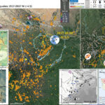
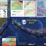
We had another earthquake in China today! This one along the northern Tian Shan Mountains, on the other side of the orogenic wedge from the earthquakes from earlier today. This M 6.3 earthquake is along a thrust fault, while the earlier M 6.5 earthquake had a strike-slip (slightly oblique) sense of motion.
Here is the USGS website for this M 6.3 earthquake.
This is my Earthquake Report for the M 6.5 earthquake from earlier today.
Here is a report from The Earth Observatory of Singapore.
Here is a report from earthquake-report.com.

Below is my interpretive poster for this earthquake

I plot the seismicity from the past month, with color representing depth and diameter representing magnitude (see legend). I also include USGS epicenters from 2007-2017 for magnitudes M ≥ 4.5.
I also include the USGS moment tensor for today’s earthquake.

  • I placed a moment tensor / focal mechanism legend on the poster. There is more material from the USGS web sites about moment tensors and focal mechanisms (the beach ball symbols). Both moment tensors and focal mechanisms are solutions to seismologic data that reveal two possible interpretations for fault orientation and sense of motion. One must use other information, like the regional tectonics, to interpret which of the two possibilities is more likely. Based upon the series of earthquakes and the mapped faults, I interpret this M 5.1 earthquake as a left-lateral strike-slip earthquake related to slip associated with the Gorda plate.
  • I also include the shaking intensity contours on the map. These use the Modified Mercalli Intensity Scale (MMI; see the legend on the map). This is based upon a computer model estimate of ground motions, different from the “Did You Feel It?” estimate of ground motions that is actually based on real observations. The MMI is a qualitative measure of shaking intensity. More on the MMI scale can be found here and here. This is based upon a computer model estimate of ground motions, different from the “Did You Feel It?” estimate of ground motions that is actually based on real observations.

    I include some inset figures in the poster.

  • In the upper left corner are two figures showing the tectonic regime (upper panel) and the major fault locations overlain upon topography (lower panel). This is from a paper that discusses how convergence in the Late Carboniferous contributed to the regional tectonics today (Han et al., 2011). I include blue stars in the general location of the M 6.3 earthquake.
  • In the upper right corner is another large scale geologic map of the region (Han et al., 2011). This map shows the different geologic units, sorted by age. Major cities and basins are labeled.
  • In the lower left corner I include a figure from Yang et al. (2008) that shows the medium scale fault mapping in this region (more detailed than the other maps on the poster). GPS velocities and slip rates calculated for various faults in the region are also plotted. Today’s earthquake appears associated with the Northern Tianshan Marginal fault, a thrust fault that crosses the Tainshan Mountains (See Li et al., 2016 map below).


  • Here is the poster from the M 6.5 earthquake.

Below are some figures that help explain today’s seismicity

  • Here is a figure from Han et al. (2011) that shows the major tectonic and geologic features. I include a subset of their very long figure caption below in blockquotes (you are welcome, for my not including their entire caption).

  • (a) The Central Asian Orogenic Belt is the tectonic assembly of continental and oceanic terranes between the European craton in the west, the Siberian craton in the east, and the North China and Tarim cratons in the south due to closure of the Paleo-Asian Ocean in the Phanerozoic (modified from Şengör et al., 1993; Jahn et al., 2000). (b) Topographic and sketch tectonic map of the western segment of the Tian Shan in China–Kyrgyzstan contiguous regions. KNTS — Kyrgyzstan North Tian Shan, KMTS — Kyrgyzstan Middle Tian Shan, KSTS — Kyrgyzstan South Tian Shan, and CSTS — Chinese South Tian Shan, AISNQF — Atbashy–Inylchek–South Nalati–Qawablak Fault, TFF — Talas–Fergana Fault, NL — Nikolaev Line, NTT — North Tarim Thrust, and NTSF — North Tian Shan Fault.

  • Here is a larger scale figure from Han et al. (2011) that shows the geology and faulting. I include their figure caption below in blockquotes.

  • Geological map of the western segment of the South Tian Shan Orogen and adjacent tectonic units (modified from IGCAGS, 2006). AISNQF — Atbashy–Inylchek–South Nalati–Qawablak Fault, TFF — Talas–Fergana Fault, NL — Nikolaev Line, and NTT — North Tarim Thrust.

  • Here is a series of figures from Yang et al. (2008) that show the earthquake fault slip rates and block rotation rates, along with Global Positioning System (GPS) analyses results. The uppermost figure is in the interpretive poster above. The middle panel shows the GPS locations and GPS transect regions. The lower two panels show GPS velocities along the transects plotted in the middle panel map. The profiles show how tectonic strain is accumulating across the faults in the region (where there are inflections in the velocities). I include their figure caption below in blockquotes.

  • Horizontal movement velocity field of the Tianshan Mountains relative to stable Eurasia plate. The arrows show movement rate and its orienta-tion with the error ellipse, at a 95% confidence level. TA, Talas-Fergana fault; KT, Kindyktash fault; BOK, Boluokenu fault; PMT, Main Pamir thrust; MAK, Markansu fault; PC, Puchang fault; MDKA, Maidan-Karatieke fault; KT, Kepingtage thrust fault; BL, Beiluntai fault; QL, Qiulitage fracture; XD, Xingdi fracture; BLK, Balikun fracture.


    Profile configuration. A, B, C, D, E, and F are longitudinal profiles across the Tianshan Mountains for Figure 4. G, H, I, J, and K are profiles across the WN-SE trending strike-slip faults for Figure 3.


    The velocity profiles across the WN-SE trending strike-slip faults in the Tianshan Mountains. G and H, the northwest and southeast sections of Talas-Fergana fault respectively; I, indyktash fault; J and K, the west and east sections of Boluokenu fault respectively. The horizontal axis represents distance from GPS sites to central point of profile, and the vertical axis shows GPS velocity.


    GPS velocity profiles across the Tianshan Mountains illustrated in Figure 2. The horizontal axis represents distance from GPS sites to central point of profile, and the vertical axis shows GPS velocity.

  • Here are some figures from Li et al. (2016) that shows detailed fault maps for this region, along with a low-angle oblique block diagram for the region outlined in yellow on the map. The M 6.3 earthquake is just to the west of the block diagram, but the structure is representative.I include their figure caption below in blockquotes.

  • Geomorphological and Tectonic features of the Tianshan Mountains. (A) Study area and earthquakes that were used for the formation of the receiver function image, which were selected from more than 500 earthquakes from a USGS database that was created during this study’s data collection. (B) Geomorphologic and tectonic features of the Tianshan Mountains, which show their segmentation with latitude and zoning with longitude, Cenozoic faults36 and Paleozoic subduction zones9,11–14,62, the asymmetry of structural deformation near the surface on both sides12, the crust’s velocity and direction from GPS data60,61, and the clockwise rotation of the Tarim Blocks22,40. The primary DEM data that were used for the geomorphological features in (B) are in the SRTM GTOPO 30 format and were provided by NASA and downloaded from http://glcf.umiacs.umd.edu in 2010.


    Cartoon map of Segment C in the Tianshan Mountains. (A) Geomorphologic features of Segment C in the Tianshan Mountains. (B) Deep structures and the driving mechanism for the uplift of the mountains during the Cenozoic. The abbreviations are the same as those in Fig. 2. The primary DEM data that were used for the geomorphological features in (A) are in the SRTM GTOPO 30 format and were provided by NASA and downloaded from http://glcf.umiacs.umd.edu in 2010.

    References:

  • Han, B-F., He, G-Q., Wang, X-C., and Guo, Z-J., 2011. Late Carboniferous collision between the Tarim and Kazakhstan–Yili terranes in the western segment of the South Tian Shan Orogen, Central Asia, and implications for the Northern Xinjiang, western China in Earth-Science Reviews, v. 109, p. 74-93
  • Kirby, E., Harkins, N., Wang, E., Shi, X., Fan, C., and Burbank, D., 2007. Slip rate gradients along the eastern Kunlun fault in Tectonics, v. 26, doi:10.1029/2006TC002033
  • Li, J. et a., 2016., Mantle Subduction and Uplift of Intracontinental Mountains: A Case Study from the Chinese Tianshan Mountains within Eurasia in Scientific Reports, DOI: 10.1038/srep28831
  • Yang, S., et al., 2008. The deformation pattern and fault rate in the Tianshan Mountains inferred from GPS observations in Science in China Series D: Earth Sciences, v. 51, no. 8, p. 1064-1080
  • Yong, L., Allen, P.A., Densmore, A.L., and Qiang, X., 2003. Evolution of the Longmen Shan Foreland Basin (Western Sichuan, China) during the Late Triassic Indosinian Orogeny in Basin Research, v. 15, p. 115-138
  • Yong, Z., HongSheng, M., Jian, L., SiDao, N., YingChun, L., and ShengJi, W./, 2009. Source mechanism of strong aftershocks (Ms≥5.6) of the 2008/05/12 Wenchuan earthquake and the implication for seismotectonics in Science in China Series D: Earth Sciences, v. 52, no. 6, p. 739-753, doi: 10.1007/s11430-009-0074-3
  • Zheng, Y-F., Xiao, W-J., and Zhao, G., 2013. Introduction to tectonics of China in Gondwana Research, v. 23, p. 1189-1206.

Earthquake Report: China!

This morning (my time) there was a shallow earthquake in western China, near a region that was shocked by an M 7.9 earthquake in 2008 (the “Wenchuan Earthquake”).
Here is the USGS website for this M 6.5 earthquake.

Below is my interpretive poster for this earthquake.

I plot the seismicity from the past month, with color representing depth and diameter representing magnitude (see legend). I also include USGS epicenters from 1917-2017 for magnitudes M ≥ 4.5.
I also include the USGS moment tensor for today’s earthquake. While it is possible that either nodal plane is correct, read below to see how I interpret today’s earthquake given the publications I include in this report (see discussion about inset figures).
This region lies along a boundary between extrusion tectonics related Kunlun and Haiyuan faults and the Longmen Shan thrust fault system. As the India subcontinent collides with Asia, central Asia is extruded to the east, forming these major strike-slip fault systems. The Haiyuan fault system experienced an M 8.3 earthquake on 1920.12.16 (shown on main map) and is one of the faults that is thought to experience superquakes and supercycles. There have been several M 7.8 earthquakes on the Kunlun fault (1932 and 2001)..

  • I placed a moment tensor / focal mechanism legend on the poster. There is more material from the USGS web sites about moment tensors and focal mechanisms (the beach ball symbols). Both moment tensors and focal mechanisms are solutions to seismologic data that reveal two possible interpretations for fault orientation and sense of motion. One must use other information, like the regional tectonics, to interpret which of the two possibilities is more likely. Based upon the series of earthquakes and the mapped faults, I interpret this M 5.1 earthquake as a left-lateral strike-slip earthquake related to slip associated with the Gorda plate.
  • I also include the shaking intensity contours on the map. These use the Modified Mercalli Intensity Scale (MMI; see the legend on the map). This is based upon a computer model estimate of ground motions, different from the “Did You Feel It?” estimate of ground motions that is actually based on real observations. The MMI is a qualitative measure of shaking intensity. More on the MMI scale can be found here and here. This is based upon a computer model estimate of ground motions, different from the “Did You Feel It?” estimate of ground motions that is actually based on real observations.

    I include some inset figures in the poster.

  • In the lower right corner I include a map showing the tectonic domains in China (Zheng et al., 2013). I place a blue star in the general location of today’s M 6.5 earthquake (as in other figures).
  • In the center left, I include a tectonic map, showing the major faults in the region (Kirby et al., 2007). The inset map is below this figure in the lower left corner. This larger scale maps shows more detail of the faults (and their study sites). Today’s earthquake happened in the mountains of Min Shan, where there are numerous north-south striking thrust faults (e.g. the Minjiang fault and the Fuya fault; the Minjian fault is labeled MJ in the upper map).
  • To the left of the Zheng et al. (2013) map is a large scale map from Yong et al., 2009. This map shows more faults at this scale. The MJ (Mijiang fault) and HY (Fuya fault) are thrust faults and probably not related to today’s earthquake. The fault labeled DKL (I cannot yet determine the name of this fault, it is not listed in their publication) is the likely culprit for today’s earthquake. Given the moment tensor, shallow depth, and orientation of the DKL fault, I interpret today’s earthquake to be a west-northwest striking left-lateral strike-slip fault.
  • In the upper right corner I include a larger scale map with the same earthquakes as plotted in the main map. I highlight the earthquakes associated with the 2008 M 7.9 Wenchuan Earthquake sequence. This earthquake triggered tens of thousands of landslides and killed many people. There was also a series of earthquakes (with an M 6.6 mainshock) to the southwest of the 2008 earthquakes, which were probably related to the Wenchuan Earthquake. To the south of today’s M 6.5 earthquake, there was a series of southward propagating thrust fault earthquakes [possibly/probably] along the Fuya fault system.


  • Here is the fault block map from Zheng et al. (2013). I include their figure caption below in blockquotes.

  • Simplified tectonic map of China showing major cratonic blocks and orogenic belts (modified after Zhao et al., 2001). Circled asterisks denote the UHP metamorphic terranes in the central orogenic belt of China (Zheng et al., 2012), which occur from west to east: Southwest Tianshan, Altyn, North Qaidam, North Qinling, and Dabie and Sulu.

  • Here are the two maps from Kirby et al. (2007). I include their figure caption below in blockquotes.

  • Tectonic map showing major and minor active faults in eastern Tibet. Abbreviations are as follows; BJ, Bailong Jiang fault; E, Elashan fault; MJ, Min Jiang fault; R, Riyueshan fault; T, Tazang fault. Epicentral locations and focal mechanism solutions of recent seismicity along the Kunlun fault are compiled from USGS (http://neic.usgs.gov/neis/epic/epic_circ.html), Harvard CMT catalog (http://www.globalcmt.org/CMTsearch.html), and Molnar and Lyon-Caen [1989]. Topographic base is generated from the Shuttle Radar Topography Mission (SRTM) data.


    Map of the eastern segment of the Kunlun fault showing location of active faults and major physiographic features. Active faults are represented by heavy lines; dashed where recent activity is inferred. Yellow River (Huang He) is shown as blue line. White boxes represent slip rate estimates (mm/yr) [Van der Woerd et al., 2002b]. Locations of new slip rate determinations are labeled in white circles (1, 2, 3). Focal mechanisms are compiled from USGS (http://neic.usgs.gov/neis/epic/epic_circ.html).

  • Here is the large scale map from Yong et al. (2009). I include their figure caption below in blockquotes.

  • Focal mechanisms of Wenchuan earthquake aftershocks with Ms≥5.6. The numbers 1-12 are the indexes of the aftershocks (1―10 are the same as Table 2). The focal mechanism of the Wenchuan main event comes from the result of Harvard CMT solution. The black lines are the Quaternary faults. The abbreviated names of the faults are the same as Figure 2.

  • Here is a figure from Yong et al. (2003) that shows the development of these large strike-slip faults (e.g. the Kunlun fault) prior to the collision of India with Asia. These faults, at this time, were thrust faults. The Longmen Shan fault system is labeled LSFB in the lower panel. I include their figure caption below in blockquotes.

  • Cartoons showing geological evolution from South China Block passive margin flaking a deep remnant ocean basin accumulating sediments of the Songpan-Ganzi Complex in (a), to oceanic closure, telescoping of the Songpan-Ganzi Complex and South China margin and formation of the Longen Shan Foreland Basin as a flexural foredeep in (G). Modified from Harrowfield (2001).

  • Here is a map from Jacha Polet, a seismologist at Cal Poly Pomona. They plot moment tensors from their compiled historic database.

  • Here is a figure from Gorum et al. (2008) that shows the epicenters from the Wenchuan Earthquake sequence, along with faults and historic earthquakes. I include their figure caption below in blockquotes.

  • Location and 12May 2008Wenchuan earthquake fault surface rupturemap, and focalmechanisms of the main earthquake (12May) and two of the major aftershocks (13 May and 25 May). Also the epicenters of historic earthquakes are indicated. The following faults are indicated: WMF: Wenchuan–Maowen fault; BF: Beichuan–Yingxiu fault; PF: Pengguan fault; JGF: Jiangyou–Guanxian fault; QCF: Qingchuan fault; HYF: Huya fault;MJF:Minjian fault based on the following sources: (Surface rupture: Xu et al., 2009a,b; Epicenter and aftershocks: USGS 2008; Historic earthquakes: Kirby et al., 2000; Li et al., 2008; Xu et al., 2009a,b).

  • Here is a figure from Gorum et al. (2008) that shows the relations between earthquake slip (proxy for ground shaking) and landslide concentration (the number of landslides per square kilometer). I include their figure caption below in blockquotes.

  • Landslide concentration in relation to the total co-seismic slip distribution of the fault rupture (co-seismic slip distribution model is from Shen et al., 2009). a: The landslide concentration; b: contour lines of landslide concentration clipped for the projected fault plane boundary; c: the co-seismic slip distribution; d: contour lines of co-seismic slip distribution.

    References:

  • Goldfinger, C., Ikeda, Y., Yeats, R.S., and Ren, J., 2013. Superquakes and Supercycles in Seismological Research Letters, v. 84, no. 1, doi: 10.1785/0220110135
  • Kirby, E., Harkins, N., Wang, E., Shi, X., Fan, C., and Burbank, D., 2007. Slip rate gradients along the eastern Kunlun fault in Tectonics, v. 26, doi:10.1029/2006TC002033
  • Yong, L., Allen, P.A., Densmore, A.L., and Qiang, X., 2003. Evolution of the Longmen Shan Foreland Basin (Western Sichuan, China) during the Late Triassic Indosinian Orogeny in Basin Research, v. 15, p. 115-138
  • Yong, Z., HongSheng, M., Jian, L., SiDao, N., YingChun, L., and ShengJi, W./, 2009. Source mechanism of strong aftershocks (Ms≥5.6) of the 2008/05/12 Wenchuan earthquake and the implication for seismotectonics in Science in China Series D: Earth Sciences, v. 52, no. 6, p. 739-753, doi: 10.1007/s11430-009-0074-3
  • Zheng, Y-F., Xiao, W-J., and Zhao, G., 2013. Introduction to tectonics of China in Gondwana Research, v. 23, p. 1189-1206.

Earthquake Report: Sulawesi, Indonesia

There was a series of earthquakes in Sulawesi, Indonesia earlier today, with a mainshock having a magnitude of M 6.8. This series of earthquakes is interesting as it does not occur on the main plate boundary fault, but on upper plate faults in the region. There is a major left-lateral strike-slip fault system to the west of these earthquakes (the Palu-Koro fault).
Part of this being interesting is that the orientation of the earthquake is oblique to some estimates of the orientation of extension in this region. The M 6.8 earthquake shows an extensional earthquake with extension oriented ~north-south. Some estimate extension in the upper plate to be northeast-southwest (Bellier et al., 2006), while others estimate extension in the upper plate to be oriented parallel to the M 6.8 earthquake (e.g. Walpersdorf et al., 1998). Spencer (2010) also documented normal faults in the upper plate that may also be correctly oriented for this M 6.8 earthquake. However, looking at the SRTM topographic data using the GeoMapApp, there is a structural grain that appears oriented to the extension estimated by Bellier et al., 2006.

  • Here are the USGS earthquake websites for this sequence.
  • 2017.05.29 14:35 M 6.8
  • 2017.05.29 14:53 M 4.7
  • 2017.05.29 15:04 M 5.1
  • 2017.05.29 15:18 M 5.1

Below is my interpretive poster for this earthquake.

I plot the seismicity from the past month, with color representing depth and diameter representing magnitude (see legend). I also include seismicity from 1917-2017 for earthquakes with magnitudes M ≥ 7.5. Here is the USGS derived Google Earth kml file I used to create this map. I show the fault plane solutions for one of these earthquakes (1996 M 7.9). The 1996 M 7.9 earthquake is oriented with the subduction fault on the north side of Sulawesi. Interestingly, there is no seismicity M ≥ 7.5 along the strike-slip systems here.

  • I placed a moment tensor / focal mechanism legend on the poster. There is more material from the USGS web sites about moment tensors and focal mechanisms (the beach ball symbols). Both moment tensors and focal mechanisms are solutions to seismologic data that reveal two possible interpretations for fault orientation and sense of motion. One must use other information, like the regional tectonics, to interpret which of the two possibilities is more likely
  • I also include the shaking intensity contours on the map. These use the Modified Mercalli Intensity Scale (MMI; see the legend on the map). This is based upon a computer model estimate of ground motions, different from the “Did You Feel It?” estimate of ground motions that is actually based on real observations. The MMI is a qualitative measure of shaking intensity. More on the MMI scale can be found here and here. This is based upon a computer model estimate of ground motions, different from the “Did You Feel It?” estimate of ground motions that is actually based on real observations.
  • I did not include the slab contours plotted (Hayes et al., 2012), which are contours that represent the depth to the subduction zone fault. These are mostly based upon seismicity. The depths of the earthquakes have considerable error and do not all occur along the subduction zone faults, so these slab contours are simply the best estimate for the location of the fault. The hypocentral depth plots this close to the location of the fault as mapped by Hayes et al. (2012).

    I include some inset figures in the poster.

  • In the lower left corner is a general tectonic map for this part of the world (Zahirovic et al., 2014). I placed a green star in the location of this M 6.8 earthquake.
  • In the lower right corner is a low-angle oblique view of the plate boundaries in the northern part of this region (Hall, 2011). The upper part of the diagram shows the opposing vergent subduction zones along that strike north-south along the Molucca Strait (Halmahera, Philippines). The lower panel shows the downgoing Australia plate along the Timor Trench and Seram Trench.. I placed a green star in the location of this M 6.8 earthquake.
  • In the upper right corner I include an inset of a seismic hazard map for this region of Indonesia. This map is from the Indonesian National Agency for Disaster Management (2011). Note the high seismic hazard associated with the Palu-Koro and Matano faults.
  • In the upper right corner I include a tectonic map showing the major fault systems and generalized plate motions (Bellier et al., 2006). Note the northeast-southwest orientation of extension in the Central Sulawesi block. I present another figure from this publication below.
  • To the right of this Bellier et al. (2006) map is another figure from that same publication. This is more generalized and shows the orientation of the faults in this region.


  • Here is the tectonic map from Bellier et al., 2006. I include their caption below in blockquote.


  • Regional geodynamic sketch that presents the present day deformation model of Sulawesi area (after Beaudouin et al., 2003) and four main deformation systems around the Central Sulawesi block, highlighting the tectonic complexity of Sulawesi. Approximate location of the Central Sulawesi block rotation pole (P) [compatible with both GPS measurements (Walpersdorf et al., 1998a) and earthquake moment tensor analyses (Beaudouin et al., 2003)], as well as the major active structures are reported. Central Sulawesi Fault System (CSFS) is formed by the Palu–Koro and Matano faults. Arrows correspond to the compression and/or extension directions deduced from both inversion and moment tensor analyses of the focal mechanisms; arrow size being proportional to the deformation rate (e.g., Beaudouin et al., 2003).We also represent the focal mechanism provided by the Harvard CMT database [CMT data base, 2005] for the recent large earthquake (Mw=6.2; 2005/1/23; lat.=0.928S; long.=120.108E). The box indicates the approximate location of the Fig. 6 that corresponds to the geological map of the Palu basin region. The bottom inset shows the SE Asia and Sulawesi geodynamic frame where arrows represent the approximate Indo-Australian and Philippines plate motions relative to Eurasia.

  • Here is the larger scale map showing the fault configuration in this region (Bellier et al., 2006)


  • Sketch map of the Cenozoic Central Sulawesi fault system. ML represents the Matano Lake, and Leboni RFZ, the Leboni releasing fault zone that connects the Palu–Koro and Matano Faults. Triangles indicate faults with reverse component (triangles on the upthrown block). On this map are reported the fault kinematic measurement sites (geographic coordinates in Table 3).

  • The extension shown in the Bellier et al. (2006) map above is largely the result of analyses conducted by and presented in Beaudouin et al. (2003). Here I present their figure where they summarize their results of block modeling using historic seismicity to drive the strain in this region. It is possible that the century of seismicity data is insufficient to account for the strain here. This may explain why the orientation of the M 6.8 earthquake is not oriented like suggested in this map below.


  • Here is a figure from Walpersdorf et al. (1998) that shows regional plate motions and the tectonic faults in the region. Note that the extension is oriented parallel to the M 6.8 extension. These data are based upon their analyses of GPS geodetic data. So, given the orientation of the M 6.8 earthquake and these data, I suspect this is the correct orientation of extension. Though, this is not consistent with the topographic data I present below.


  • Distribution of the calk alkalic potassic (CAK) volcanism in Sulawesi. In the west arm this volcanism is restricted to the central part of the arm, while east of the Palu–Koro fault zone CAK volcanism is distributed across a NW–SE 200 km wide belt extending from north Sulawesi to the Una-Una Island. The two synthetic cross sections illustrate the contrasting distribution of this volcanism on both sides of the Palu–Koro fault zone. Extension of the Sula-Buton=north Sulawesi arc is speculative. The double arrow illustrates extension in the Gulf of Gorontalo. Dashed lines in cross sections indicate the presence at depth of the remnant subducted Tethys oceanic crust.

  • This is smaller scale tectonic map of the region (Zahirovic et al., 2014).

  • Regional tectonic setting with plate boundaries (MORs/transforms = black, subduction zones = teethed red) from Bird (2003) and ophiolite belts representing sutures modified from Hutchison (1975) and Baldwin et al. (2012). West Sulawesi basalts are from Polvé et al. (1997), fracture zones are from Matthews et al. (2011) and basin outlines are from Hearn et al. (2003). ANI – Andaman and Nicobar Islands, BD– Billiton Depression, Ba – Bangka Island, BI – Belitung (Billiton) Island, BiS – Bismarck Sea, BP – Benham Plateau, CaR – Caroline Ridge, CS – Celebes Sea, DG– Dangerous Grounds, EauR – Eauripik Ridge, FIN – Finisterre Terrane, GoT – Gulf of Thailand, GR– Gagua Ridge, HAL– Halmahera, HBa – Huatung Basin, KB–Ketungau Basin, KP – Khorat Platform, KT – Kiilsgaard Trough, LS – Luconia Shoals, MacB – Macclesfield Bank, ManTr – Manus Trench, MaTr – Mariana Trench, MB– Melawi Basin, MDB– Minami Daito Basin, MG– Mangkalihat, MIN – Mindoro, MN– Mawgyi Nappe, MoS – Molucca Sea, MS– Makassar Straits, MTr – Mussau Trench, NGTr – New Guinea Trench, NI – Natuna Islands, ODR– Oki Daito Ridge, OJP –Ontong Java Plateau, OSF – Owen Stanley Fault, PAL – Palawan, PhF – Philippine Fault, PT – Paternoster Platform, PTr – Palau Trench, PVB – Parece Vela Basin, RB – Reed Bank, RMF– Ramu-Markham Fault, RRF – Red River fault, SEM– Semitau, ShB – Shikoku Basin, Sol. Sea – Solomon Sea, SPK – Sepik, SPT – abah–Palawan Trough, STr – Sorol Trough, Sul – Sulawesi, SuS – Sulu Sea, TPAA– Torricelli–Prince Alexander Arc, WB–West Burma, WCT–W Caroline Trough, YTr –Yap Trough.

  • Here is a map from Spencer (2010). Today’s M 6.8 occurred along the cross section A-A.’


  • Elevation and shaded-relief maps and topographic cross sections derived from the SRTM DEM using GeoMapApp©. (A) Map of the Sulawesi and surrounding areas, with bathymetry derived from the Marine Geoscience Data System bathymetry database. Geologic features from Hamilton (1979) and Silver et al. (1983). (B) Map of central Sulawesi (location in A) showing inferred detachment faults (double ticks on hanging wall) and high-angle faults (red lines). (C) Map of the Tokorondo massif (location in B) showing inferred detachment fault and high-angle faults. (D) Topographic cross sections (location in C) of Tokorondo massif.

  • Here is a map from the GeoMapApp, using Global Multi-Resolution Topography (GMRT) topographic data (Ryan et al., 2009). Note the north-northwest structural grain. These appear to be normal faults oriented with a east-northeast/west-southwest extension from Bellier et al. (2006). This is the same general region as presented in the Spencer (2010) map above. Note the two large rounded plateau-highlands and the low lying basins (lakes are not outlined in this map).


References:

  • Bellier, O., Se´brier, M., Seward, D., Beaudouin, T., Villeneuve, M., and Putranto, E., 2006. Fission track and fault kinematics analyses for new insight into the Late Cenozoic tectonic regime changes in West-Central Sulawesi (Indonesia) in Tectonophysics, v. 413, p. 201-220.
  • Benz, H.M., Herman, Matthew, Tarr, A.C., Hayes, G.P., Furlong, K.P., Villaseñor, Antonio, Dart, R.L., and Rhea, Susan, 2011. Seismicity of the Earth 1900–2010 New Guinea and vicinity: U.S. Geological Survey Open-File Report 2010–1083-H, scale 1:8,000,000.
  • Hall, R., 2011. Australia-SE Asia collision: plate tectonics and crustal flow in Geological Society, London, Special Publications 2011; v. 355; p. 75-109 doi: 10.1144/SP355.5
  • Hayes, G.P., Wald, D.J., and Johnson, R.L., 2012. Slab1.0: A three-dimensional model of global subduction zone geometries in, J. Geophys. Res., 117, B01302, doi:10.1029/2011JB008524
  • Hayes, G.P., Smoczyk, G.M., Benz, H.M., Villaseñor, Antonio, and Furlong, K.P., 2015. Seismicity of the Earth 1900–2013, Seismotectonics of South America (Nazca Plate Region): U.S. Geological Survey Open-File Report 2015–1031–E, 1 sheet, scale 1:14,000,000, http://dx.doi.org/10.3133/ofr20151031E.
  • Ryan, W.B.F., S.M. Carbotte, J.O. Coplan, S. O’Hara, A. Melkonian, R. Arko, R.A. Weissel, V. Ferrini, A. Goodwillie, F. Nitsche, J. Bonczkowski, and R. Zemsky, 2009. Global Multi-Resolution Topography synthesis, Geochem. Geophys. Geosyst., 10, Q03014, doi: 10.1029/2008GC002332
  • Walpersdorf, A., Rangin, C., and Vigny, C., 1998. GPS compared to long-term geologic motion of the north arm of Sulawesi in EPSL, v. 159, p. 47-55.
  • Zahirovic, S., Seton, M., and Müller, R.D., 2014. The Cretaceous and Cenozoic tectonic evolution of Southeast Asia in Solid Earth, v. 5, p. 227-273, doi:10.5194/se-5-227-2014

Earthquake Report: Philippines

I put these together earlier this week for my classes and finally have a moment to write about these earthquakes. The Philippines region has been quite active lately, as it frequently is.

I show below a series of earthquakes from the past ~30 days. These earthquakes occurred in 4 different regions and 3 different tectonic settings. These are probably unrelated to each other, but it is difficult to really know without further analyses.

After I made these posters, there was an earthquake with a magnitude of M 5.8 on the island of Mindanao (I include the USGS link below), possibly associated with the Davao River fault (the closest fault mapped in this region).

Here are the USGS websites for these earthquakes.

I took a look at the seismicity from the past century. Here are Google Earth kml files from the USGS website for earthquakes from 1917-2017 with magnitudes M ≥ 7.0 and M ≥ 7.5.

Below is my interpretive poster for this earthquake.

I plot the seismicity from the past month, with color representing depth and diameter representing magnitude (see legend). I include the USGS epicenters for earthquakes from 1917-2017 with magnitudes M ≥ 7.5.

  • A review of the basic base map variations and data that I use for the interpretive posters can be found on the Earthquake Reports page. I have improved these posters over time and some of this background information applies to the older posters.
  • Some basic fundamentals of earthquake geology and plate tectonics can be found on the Earthquake Plate Tectonic Fundamentals page.
  • I placed a moment tensor / focal mechanism legend on the poster. There is more material from the USGS web sites about moment tensors and focal mechanisms (the beach ball symbols). Both moment tensors and focal mechanisms are solutions to seismologic data that reveal two possible interpretations for fault orientation and sense of motion. One must use other information, like the regional tectonics, to interpret which of the two possibilities is more likely.
  • I also include the shaking intensity contours on the map. These use the Modified Mercalli Intensity Scale (MMI; see the legend on the map). This is based upon a computer model estimate of ground motions, different from the “Did You Feel It?” estimate of ground motions that is actually based on real observations. The MMI is a qualitative measure of shaking intensity. More on the MMI scale can be found here and here. This is based upon a computer model estimate of ground motions, different from the “Did You Feel It?” estimate of ground motions that is actually based on real observations.
  • I include the slab contours plotted (Hayes et al., 2012), which are contours that represent the depth to the subduction zone fault. These are mostly based upon seismicity. The depths of the earthquakes have considerable error and do not all occur along the subduction zone faults, so these slab contours are simply the best estimate for the location of the fault.

    I include some inset figures in the poster.

  • In the upper left corner is a figure from Hall, 2011. This shows the plate tectonic configuration in the equatorial Pacific. Note how the upper panel shows a west dipping slab on the east side of the Philippines. Note the contrast in the center panel (Halmahera), where the eastern fault is dipping to the east (westward vergent) and the western fault is dipping to the west (eastward vergent). This region near Halmahera forms the Molucca Strait, one of the most tectonically active areas in this region.
  • In the upper right corner is a map showing the regional faults from Noda (2013). The Philippine and Sibuyan Sea faults are “forearc sliver” faults that accommodate oblique convergence between the Philippine Sea and Sunda plates. The M 5.9 epicenter is designated by a red star. The Manila trench (MT; northernmost east-dipping subduction zone) and the Philippine trench (PT; easternmost west-dipping subduction zone) are major players here. The high velocity plate motion vectors (in mm/yr) show the relative plate motions and the possible source of hi frequency seismicity.
  • In the lower left corner I include a map showing the seismicity and tectonic plate boundary faults for this region (Smoczyk et al., 2013). Earthquakes are plotted with color representing depth and diameter representing magnitude (see legend).


  • In the above poster, I choose 4 earthquakes for which to plot the MMI intensity.
  • The easternmost two are earthquakes related to the subduction of the Philippine Sea plate.
  • The northwesternmost earthquake series (largest M = 5.9) is interesting and mysterious. There is a left-lateral forearc sliver fault (Philippine fault) that parallels the Philippine trench. Internal deformation in the upper plate is accommodated by a complicated series of other strike-slip faults. In the region near Manila, there is a north-south striking right-lateral Mirikina Valley fault system. The MV fault trends south from Manila into the region of the M 5.9 earthquake. This fault seems to terminate in a northeast-southwest trending zone of “extension and young volcanism” (Nelson et al., 2000). Further to the south is an east-west striking left-lateral Lubang fault. This may be an extension of the Sibuyan Sea fault (Noda, 2013), a splay of the Philippine fault. If we look at the moment tensor for the M 5.5 and 5.9 earthquakes, the nodal planes suggest either NE striking left-lateral or NW striking right-lateral motion. This does not fit the orientation nor sense of motion for any of the mapped faults in the region. It is possible that these earthquakes are related to the extensional rifting instead. The moment tensor for the M 5.1 earthquake here shows an extensional beach ball. The orientation is not completely correct based upon the Nelson et al. (2000) figure, but there are no faults shown on their map.
  • The southwestern earthquakes from March (both M 5.6) are also interesting. The epicenters show locations on north Sulawesi, part of Indonesia. There is a NW striking left-lateral strike-slip faults mapped to the west and east of these earthquakes. However, the moment tensor shows that this would be a right-lateral fault in that orientation. The NW striking reverse fault is also equally challenging to interpret. Needless to say, this is a tectonically complicated region.

Below is the interpretive poster for the 08 April 2017 M 5.9 earthquake.


  • This is the low-angle oblique view of the region (Hall, 2011).

  • 3D cartoon of plate boundaries in the Molucca Sea region modified from Hall et al. (1995). Although seismicity identifies a number of plates there are no continuous boundaries, and the Cotobato, North Sulawesi and Philippine Trenches are all intraplate features. The apparent distinction between different crust types, such as Australian continental crust and oceanic crust of the Philippine and Molucca Sea, is partly a boundary inactive since the Early Miocene (east Sulawesi) and partly a younger but now probably inactive boundary of the Sorong Fault. The upper crust of this entire region is deforming in a much more continuous way than suggested by this cartoon.

  • Here is the fault map for the region on the Island of Luzon (where Manila is located) from Nelson et al. (2000). The panel on the right (B) shows the Marikina Valley fault system (MV) and the Lubang fault. The MV is a right-lateral strike slip fault and the Lubang fault is a left-lateral strike-slip fault.

  • Tectonic setting of the Marikina Valley fault system (MV) in central Luzon, the Philippines. Diagram A shows subduction zone trenches by barbed lines, other faults with high rates of Quaternary activity by heavy black lines. White dots show locations of recent earthquakes on the Philippine fault in Luzon (M 7.8; 1990) and the Aglubang River fault in Mindoro (M 7.1; 1994). Diagram B shows how the Marikina Valley pull-apart basin (MV) may have been formed through extension caused by clockwise rotation (dashed circle) and shearing of central Luzon, which is caught between two active left-lateral strike-slip faults—the Philippine fault (Nakata et al., 1977; Barrier et al., 1991; Ringenbach et al., 1993; Aurelio et al., 1993) and the Lubang fault. A zone of extension and young volcanism south of the fault system has also influenced the structural development of the valley (Fo¨rster et al., 1990; Defant et al., 1988).

  • Here is the map from Noda (2013) that shows various strike slip faults associated with subduction zones.

  • Modern examples of trench-linked strike-slip faults. (A) The Median Tectonic Line (MTL) active fault system in southwestern Japan, related to oblique subduction of the Philippine Sea Plate (PS) along the Nankai Trough (NT). (B) The Great Sumatra Fault system (GSF) along the Java–Sumatra Trench (JST). (C) Strike-slip faults in Alaska. Fault names: DF, Denali; BRF, Boarder Ranges; CSEF, Chugach St. Elias; FF, Fairweather; TF, Transition. (D) The Philippine Fault system (PF). Abbreviations: SSF, Sibuyan Sea Fault; MT, Manila Trench; PT, Philippine Trench; ELT, East Luzon Trough. Plate names: AM, Amur; OK, Okhotsk; PS, Philippine Sea; AU, Australian; SU, Sundaland; NA, North American; PA, Pacific; YMC, Yukutat microcontinent. Black and purple lines are subduction zones and trench-linked strike-slip faults, respectively. All maps were drawn using SRTM and GEBCO with plate boundary data [30]. Blue arrows indicate the direction and velocity of relative plate motion (mm yr-1) based on [31].

The USGS Maps and Cross-Sections

  • Here is the map from Smocyk et al., 2013, followed by the legend. The entire poster is here (92 MB pdf).


  • Below are two cross sections that show the subduction zone seismicity, followed by the legend. The location of these cross sections are labeled on the map above.


  • This map shows the seismic hazard for this region. The color represents the likelihood of any region experiencing ground shaking of a particular magnitude. The scale is “Peak Ground Acceleration.” Units are m/s^2. Purple represents gravitational acceleration of 1 g, gravity at Earth’s surface. Note how most of the earthquakes were in the region of higher likely ground shaking, except for the Sulawesi earthquakes.

  • In January of this year, there was an M 7.3 earthquake in the Celebes Sea south of the Philippines. Below is my interpretive map for that earthquake. I also present the same poster with 1917-2017 seismicity for earthquakes M ≥ 6.5. Here is my earthquake report for this M 7.3 earthquake. I include more background information for the Molucca Strait region on this page.


References:

    Basic & General References

  • Frisch, W., Meschede, M., Blakey, R., 2011. Plate Tectonics, Springer-Verlag, London, 213 pp.
  • Hayes, G., 2018, Slab2 – A Comprehensive Subduction Zone Geometry Model: U.S. Geological Survey data release, https://doi.org/10.5066/F7PV6JNV.
  • Holt, W. E., C. Kreemer, A. J. Haines, L. Estey, C. Meertens, G. Blewitt, and D. Lavallee (2005), Project helps constrain continental dynamics and seismic hazards, Eos Trans. AGU, 86(41), 383–387, , https://doi.org/10.1029/2005EO410002. /li>
  • Jessee, M.A.N., Hamburger, M. W., Allstadt, K., Wald, D. J., Robeson, S. M., Tanyas, H., et al. (2018). A global empirical model for near-real-time assessment of seismically induced landslides. Journal of Geophysical Research: Earth Surface, 123, 1835–1859. https://doi.org/10.1029/2017JF004494
  • Kreemer, C., J. Haines, W. Holt, G. Blewitt, and D. Lavallee (2000), On the determination of a global strain rate model, Geophys. J. Int., 52(10), 765–770.
  • Kreemer, C., W. E. Holt, and A. J. Haines (2003), An integrated global model of present-day plate motions and plate boundary deformation, Geophys. J. Int., 154(1), 8–34, , https://doi.org/10.1046/j.1365-246X.2003.01917.x.
  • Kreemer, C., G. Blewitt, E.C. Klein, 2014. A geodetic plate motion and Global Strain Rate Model in Geochemistry, Geophysics, Geosystems, v. 15, p. 3849-3889, https://doi.org/10.1002/2014GC005407.
  • Meyer, B., Saltus, R., Chulliat, a., 2017. EMAG2: Earth Magnetic Anomaly Grid (2-arc-minute resolution) Version 3. National Centers for Environmental Information, NOAA. Model. https://doi.org/10.7289/V5H70CVX
  • Müller, R.D., Sdrolias, M., Gaina, C. and Roest, W.R., 2008, Age spreading rates and spreading asymmetry of the world’s ocean crust in Geochemistry, Geophysics, Geosystems, 9, Q04006, https://doi.org/10.1029/2007GC001743
  • Pagani,M. , J. Garcia-Pelaez, R. Gee, K. Johnson, V. Poggi, R. Styron, G. Weatherill, M. Simionato, D. Viganò, L. Danciu, D. Monelli (2018). Global Earthquake Model (GEM) Seismic Hazard Map (version 2018.1 – December 2018), DOI: 10.13117/GEM-GLOBAL-SEISMIC-HAZARD-MAP-2018.1
  • Silva, V ., D Amo-Oduro, A Calderon, J Dabbeek, V Despotaki, L Martins, A Rao, M Simionato, D Viganò, C Yepes, A Acevedo, N Horspool, H Crowley, K Jaiswal, M Journeay, M Pittore, 2018. Global Earthquake Model (GEM) Seismic Risk Map (version 2018.1). https://doi.org/10.13117/GEM-GLOBAL-SEISMIC-RISK-MAP-2018.1
  • Zhu, J., Baise, L. G., Thompson, E. M., 2017, An Updated Geospatial Liquefaction Model for Global Application, Bulletin of the Seismological Society of America, 107, p 1365-1385, https://doi.org/0.1785/0120160198
  • Specific References

  • Bock et al., 2003. Crustal motion in Indonesia from Global Positioning System measurements in JGR, v./ 108, no. B8, 2367, doi:10.1029/2001JB000324
  • Hall, R., 2011. Australia–SE Asia collision: plate tectonics and crustal flow in Hall, R., Cottam, M. A. &Wilson, M. E. J. (eds) The SE Asian Gateway: History and Tectonics of the Australia–Asia Collision. Geological Society, London, Special Publications, 355, 75–109.
  • Hayes, G.P., Wald, D.J., and Johnson, R.L., 2012. Slab1.0: A three-dimensional model of global subduction zone geometries in, J. Geophys. Res., 117, B01302, doi:10.1029/2011JB008524
  • McCaffrey, R., Silver, E.A., and Raitt, R.W., 1980. Crustal Structure of the Molucca Sea Collision Zone, Indonesia in The Tectonic and Geologic Evolution of Southeast Asian Seas and Islands-Geophysical Monograph 23, p. 161-177.
  • Nelson, A.R., Personius, S.F., Rimando, R.E., Punongbayan, R.S., Tungol, N, Mirabueno, H., and Rasdas, A., 2000. Multiple Large Earthquakes in the Past 1500 Years on a Fault in Metropolitan Manila, the Philippines in BSSA vol. 90, p. 73-85.
  • Noda, A., 2013. Strike-Slip Basin – Its Configuration and Sedimentary Facies in Mechanism of Sedimentary Basin Formation – Multidisciplinary Approach on Active Plate Margins http://www.intechopen.com/books/mechanism-of-sedimentarybasin-formation-multidisciplinary-approach-on-active-plate-margins http://dx.doi.org/10.5772/56593
  • Smoczyk, G.M., Hayes, G.P., Hamburger, M.W., Benz, H.M., Villaseñor, Antonio, and Furlong, K.P., 2013. Seismicity of the Earth 1900–2012 Philippine Sea plate and vicinity: U.S. Geological Survey Open-File Report 2010–1083-M, 1 sheet, scale 1:10,000,000.
  • Waltham et al., 2008. Basin formation by volcanic arc loading in GSA Special Papers 2008, v. 436, p. 11-26.
  • Zahirovic et al., 2014. The Cretaceous and Cenozoic tectonic evolution of Southeast Asia in Solid Earth, v. 5, p. 227-273, doi:10.5194/se-5-227-2014.

Return to the Earthquake Reports page.

Earthquake Report: Banda Sea

Earlier this week there was a moderate earthquake along a strike-slip fault that appears to adjoin the Banda/Timor/Java Arc with New Guinea. This strike-slip fault appears to cross oblique to the subduction zone that forms the Timor Trench to the south and the Seram Trench to the north. Various researchers portray the faulting in this region differently. Given earthquake moment tensor and focal mechanism from the USGS, this earthquake supports the interpretation that this fault system is left-lateral (synistral) strike-slip. A focal mechanism from an earthquake in 1938 (magnitude M 8.5) provides evidence that is a little more confusing. But, this region is a complicated region.
UPDATE: 2017.03.05 (23:00 local time): Interesting, I was reading my tweet after Lila Lisle noticed a mistake. I fixed that, but later realized that the possible fault in the downgoing plate is not the Sorog fault, but a fault that might intersect with the Sorong fault. I did not delete the tweet since this mistake is a topic of conversation and not really a key part of the story.
Here is the USGS earthquake website for this M 5.5 earthquake.

Here are the USGS websites for the major earthquakes in this region from the past century.

Below is my interpretive poster for this earthquake.

I plot the seismicity from the past month, with color representing depth and diameter representing magnitude (see legend). I also include seismicity from 1917-2017 for earthquakes with magnitudes M ≥ 7.0. I show the fault plane solutions for some of these earthquakes.

  • moment tensors for 2005, 2012, and 2017 (USGS)
  • focal mechanisms for 1987 (USGS) and 1938 (Okal and Reymond, 2003)
  • The fault plane solutions for the 1963, 1987, 2005, and 2012 earthquakes are all very similar to the 2017 M 5.5. However, these earthquakes are form two depth “populations.” The 1963 and 1987 earthquakes are at ~65 km depth, while the 2005, 2012, and 2017 are between 150-200 km. There are some earthquakes that are much shallower depth eastward along this possibly strike-slip fault. Near where this fault comes on land at the base of the Bird’s Head in New Guinea, there are some earthquakes from the past couple of decades that also have strike-slip fault–plane solutions. The earthquake depths along this Sorong fault (Hall, 2011) appear to show that the Sorong fault is active beneath the Sunda plate. The 1938 earthquake may be the result of some form of strain partitioned faulting(?). Alternatively, these earthquakes may be unrelated to the Sorong fault. There may be some internal structure in the Australia plate that is interacting with the subduction zones or other faults (some preexisting structure that is optimally oriented to reactivate with the .
  • I placed a moment tensor / focal mechanism legend on the poster. There is more material from the USGS web sites about moment tensors and focal mechanisms (the beach ball symbols). Both moment tensors and focal mechanisms are solutions to seismologic data that reveal two possible interpretations for fault orientation and sense of motion. One must use other information, like the regional tectonics, to interpret which of the two possibilities is more likely
  • I also include the shaking intensity contours on the map. These use the Modified Mercalli Intensity Scale (MMI; see the legend on the map). This is based upon a computer model estimate of ground motions, different from the “Did You Feel It?” estimate of ground motions that is actually based on real observations. The MMI is a qualitative measure of shaking intensity. More on the MMI scale can be found here and here. This is based upon a computer model estimate of ground motions, different from the “Did You Feel It?” estimate of ground motions that is actually based on real observations.
  • I include the slab contours plotted (Hayes et al., 2012), which are contours that represent the depth to the subduction zone fault. These are mostly based upon seismicity. The depths of the earthquakes have considerable error and do not all occur along the subduction zone faults, so these slab contours are simply the best estimate for the location of the fault. The hypocentral depth plots this close to the location of the fault as mapped by Hayes et al. (2012).

    I include some inset figures in the poster.

  • In the upper left corner is a general tectonic map for this part of the world. I placed a green star in the location of this M 5.5 earthquake (Zahirovic et al., 2014).
  • In the upper right corner is a low-angle oblique view of the plate boundaries in the northern part of this region (Hall, 2011). The upper part of the diagram shows the opposing vergent subduction zones along that strike north-south along the Molucca Strait (Halmahera, Philippines). The lower panel shows the downgoing Australia plate along the Timor Trench and Seram Trench. Note the location of the Bird’s Head, the northwestern part of New Guinea. I have also labeled this region in the main map for comparison. The strike-slip fault at the northern boundary of New Guinea is the Sorong fault and this is labeled in this Hall (2011) figure.
  • Below the Hall (2011) figure is a figure from Baldwin et al. (2012) that shows the regional seismicity and faulting as they are related to different geologic types in New Guinea. I placed a green star in the location of this M 5.5 earthquake.
  • In the lower right corner is a part of the USGS Poster that reviews the seismicity of this region for the past century or so (Benz et a., 2011). The map shows seismicity with depth, along with some cross section locations. I place a green star at the location of this M 5.5 earthquake. I present three of the cross sections from this poster, A-A’, B-B’, and C-C.’ Of particular interest is the section B-B’ because this is placed near the M 5.5 earthquake. I have placed a green star that represents the hypocentral location on cross section B-B.’ The hypocentral depth suggests this M 5.5 earthquake is in the downgoing Australia plate slab.
  • In the lower left corner is a diagram showing the subducting Australia plate at the Java Trench (Yves Descatoire).
  • To the right of the Java Trench figure presents a detailed view of the faulting along the eastern Java and western Timor trenches (Hangesh and Whitney, 2016). They present evidence for oblique motion along the Timor trough. And present evidence for a backthrust on the northern side of Timor and the Indonesia islands east of Java.


  • Here is the map from Baldwin et al. (2012)

  • Tectonic maps of the New Guinea region. (a) Seismicity, volcanoes, and plate motion vectors. Plate motion vectors relative to the Australian plate are surface velocity models based on GPS data, fault slip rates, and earthquake focal mechanisms (UNAVCO, http://jules.unavco.org/Voyager/Earth). Earthquake data are sourced from the International Seismological Center EHB Bulletin (http://www.isc.ac.uk); data represent events from January 1994 through January 2009 with constrained focal depths. Background image is generated from http://www.geomapapp.org. Abbreviations: AB, Arafura Basin; AT, Aure Trough; AyT, Ayu Trough; BA, Banda arc; BSSL, Bismarck Sea seismic lineation; BH, Bird’s Head; BT, Banda Trench; BTFZ, Bewani-Torricelli fault zone; DD, Dayman Dome; DEI, D’Entrecasteaux Islands; FP, Fly Platform; GOP, Gulf of Papua; HP, Huon peninsula; LA, Louisiade Archipelago; LFZ, Lowlands fault zone; MaT, Manus Trench; ML, Mt. Lamington; MT, Mt. Trafalgar; MuT, Mussau Trough; MV, Mt. Victory; MTB, Mamberamo thrust belt; MVF, Managalase Plateau volcanic field; NBT, New Britain Trench; NBA, New Britain arc; NF, Nubara fault; NGT, New Guinea Trench; OJP, Ontong Java Plateau; OSF, Owen Stanley fault zone; PFTB, Papuan fold-and-thrust belt; PP, Papuan peninsula; PRi, Pocklington Rise; PT, Pocklington Trough; RMF, Ramu-Markham fault; SST, South Solomons Trench; SA, Solomon arc; SFZ, Sorong fault zone; ST, Seram Trench; TFZ, Tarera-Aiduna fault zone; TJ, AUS-WDKPAC triple junction; TL, Tasman line; TT, Trobriand Trough;WD, Weber Deep;WB, Woodlark Basin;WFTB, Western (Irian) fold-and-thrust belt; WR,Woodlark Rift; WRi, Woodlark Rise; WTB, Weyland thrust; YFZ, Yapen fault zone.White box indicates the location shown in Figure 3. (b) Map of plates, microplates, and tectonic blocks and elements of the New Guinea region. Tectonic elements modified after Hill & Hall (2003). Abbreviations: ADB, Adelbert block; AOB, April ultramafics; AUS, Australian plate; BHB, Bird’s Head block; CM, Cyclops Mountains; CWB, Cendrawasih block; CAR, Caroline microplate; EMD, Ertsberg Mining District; FA, Finisterre arc; IOB, Irian ophiolite belt; KBB, Kubor & Bena blocks (including Bena Bena terrane); LFTB, Lengguru fold-and-thrust belt; MA, Mapenduma anticline; MB, Mamberamo Basin block; MO, Marum ophiolite belt; MHS, Manus hotspot; NBS, North Bismarck plate; NGH, New Guinea highlands block; NNG, Northern New Guinea block; OKT, Ok Tedi mining district; PAC, Pacific plate; PIC, Porgera intrusive complex; PSP, Philippine Sea plate; PUB, Papuan Ultramafic Belt phiolite; SB, Sepik Basin block; SDB, Sunda block; SBS, South Bismarck plate; SIB, Solomon Islands block; WP, Wandamen p ninsula; WDK, Woodlark microplate; YQ, Yeleme quarries.

  • Here is the tectonic map from Hangesh and Whitney (2016)

  • Illustration of major tectonic elements in triple junction geometry: tectonic features labeled per Figure 1; seismicity from ISC-GEM catalog [Storchak et al., 2013]; faults in Savu basin from Rigg and Hall [2011] and Harris et al. [2009]. Purple line is edge of Australian continental basement and fore arc [Rigg and Hall, 2011]. Abbreviations: AR = Ashmore Reef; SR = Scott Reef; RS = Rowley Shoals; TCZ = Timor Collision Zone; ST = Savu thrust; SB = Savu Basin; TT = Timor thrust; WT =Wetar thrust; WASZ = Western Australia Shear Zone. Open arrows indicate relative direction of motion; solid arrows direction of vergence.

  • Here is the Audley (2011) cross section showing how the backthrust relates to the subduction zone beneath Timor. I include their figure caption in blockquote below.

  • Cartoon cross section of Timor today, (cf. Richardson & Blundell 1996, their BIRPS figs 3b, 4b & 7; and their fig. 6 gravity model 2 after Woodside et al. 1989; and Snyder et al. 1996 their fig. 6a). Dimensions of the filled 40 km deep present-day Timor Tectonic Collision Zone are based on BIRPS seismic, earthquake seismicity and gravity data all re-interpreted here from Richardson & Blundell (1996) and from Snyder et al. (1996). NB. The Bobonaro Melange, its broken formation and other facies are not indicated, but they are included with the Gondwana mega-sequence. Note defunct Banda Trench, now the Timor TCZ, filled with Australian continental crust and Asian nappes that occupy all space between Wetar Suture and the 2–3 km deep deformation front north of the axis of the Timor Trough. Note the much younger decollement D5 used exactly the same part of the Jurassic lithology of the Gondwana mega-sequence in the older D1 decollement that produced what appears to be much stronger deformation.

  • Here is a figure showing the regional geodetic motions (Bock et al., 2003). I include their figure caption below as a blockquote.

  • Topographic and tectonic map of the Indonesian archipelago and surrounding region. Labeled, shaded arrows show motion (NUVEL-1A model) of the first-named tectonic plate relative to the second. Solid arrows are velocity vectors derived from GPS surveys from 1991 through 2001, in ITRF2000. For clarity, only a few of the vectors for Sumatra are included. The detailed velocity field for Sumatra is shown in Figure 5. Velocity vector ellipses indicate 2-D 95% confidence levels based on the formal (white noise only) uncertainty estimates. NGT, New Guinea Trench; NST, North Sulawesi Trench; SF, Sumatran Fault; TAF, Tarera-Aiduna Fault. Bathymetry [Smith and Sandwell, 1997] in this and all subsequent figures contoured at 2 km intervals.

References:

  • Audley-Charles, M.G., 1986. Rates of Neogene and Quaternary tectonic movements in the Southern Banda Arc based on micropalaeontology in: Journal of fhe Geological Society, London, Vol. 143, 1986, pp. 161-175.
  • Audley-Charles, M.G., 2011. Tectonic post-collision processes in Timor, Hall, R., Cottam, M. A. &Wilson, M. E. J. (eds) The SE Asian Gateway: History and Tectonics of the Australia–Asia Collision. Geological Society, London, Special Publications, 355, 241–266.
  • Baldwin, S.L., Fitzgerald, P.G., and Webb, L.E., 2012. Tectonics of the New Guinea Region in Annu. Rev. Earth Planet. Sci., v. 41, p. 485-520.
  • Benz, H.M., Herman, Matthew, Tarr, A.C., Hayes, G.P., Furlong, K.P., Villaseñor, Antonio, Dart, R.L., and Rhea, Susan, 2011. Seismicity of the Earth 1900–2010 New Guinea and vicinity: U.S. Geological Survey Open-File Report 2010–1083-H, scale 1:8,000,000.
  • Hall, R., 2011. Australia-SE Asia collision: plate tectonics and crustal flow in Geological Society, London, Special Publications 2011; v. 355; p. 75-109 doi: 10.1144/SP355.5
  • Hangesh, J. and Whitney, B., 2014. Quaternary Reactivation of Australia’s Western Passive Margin: Inception of a New Plate Boundary? in: 5th International INQUA Meeting on Paleoseismology, Active Tectonics and Archeoseismology (PATA), 21-27 September 2014, Busan, Korea, 4 pp.
  • Hayes, G.P., Wald, D.J., and Johnson, R.L., 2012. Slab1.0: A three-dimensional model of global subduction zone geometries in, J. Geophys. Res., 117, B01302, doi:10.1029/2011JB008524
  • Hayes, G.P., Smoczyk, G.M., Benz, H.M., Villaseñor, Antonio, and Furlong, K.P., 2015. Seismicity of the Earth 1900–2013, Seismotectonics of South America (Nazca Plate Region): U.S. Geological Survey Open-File Report 2015–1031–E, 1 sheet, scale 1:14,000,000, http://dx.doi.org/10.3133/ofr20151031E.
  • Okal, E. A., & Reymond, D., 2003. The mechanism of great Banda Sea earthquake of 1 February 1938: applying the method of preliminary determination of focal mechanism to a historical event in EPSL, v. 216, p. 1-15.
  • Zahirovic, S., Seton, M., and Müller, R.D., 2014. The Cretaceous and Cenozoic tectonic evolution of Southeast Asia in Solid Earth, v. 5, p. 227-273, doi:10.5194/se-5-227-2014

Earthquake Report: Makran subduction zone (Pakistan)!

There was a good sized earthquake along the Makran subduction zone. This subduction zone is a convergent plate boundary where the Arabia plate subducts (goes beneath) northwards under the Eurasia plate. There has been one aftershock reported by the USGS. These earthquakes are in the region of an earthquake with a magnitude of M 8.1 from 1945, which generated a large tsunami in the region. There are some reports of damage. There was an aftershock to the 1945 earthquake in 1947, when there was an earthquake with a magnitude of M 6.8 occurred in almost the same location as this 2017 earthquake. However, the 2017 M 6.3 is much deeper. There is some indication that there may be underplated sediment (sediment that is scraped off of the downgoing plate and attached to the upper plate). Perhaps the 1945 and 1947 earthquakes are on a shallower fault. Perhaps their locations are poorly resolved due to poor seismometer instrument coverage at that time.

This is also a region that experienced some effects from an earthquake further to the north in 2013. On 2013.09.24 there was an earthquake with a magnitude of M 7.7 that caused ground shaking throughout the region, as well as an interesting feature that arose from the seafloor along the continental shelf (what this feature is called is in debate; some called it a mud volcano). Here is my brief report on the 2013 earthquake.

    Here are the USGS websites for these earthquakes.

  • 2017.02.07 22:03 (UTC) M 6.3
  • 2017.02.08 11:02 (UTC) M 5.2
  • 2013.09.24 11:29 (UTC) M 7.7
  • 1945.11.27 21:56 (UTC) M 8.1

Below I present my interpretive poster for this M 6.3 earthquake. I include epicenters for earthquakes from the past century with magnitudes M ≥ 6.0. Here is the kml I created from the USGS earthquakes website.

  • I placed a moment tensor / focal mechanism legend on the poster. There is more material from the USGS web sites about moment tensors and focal mechanisms (the beach ball symbols). Both moment tensors and focal mechanisms are solutions to seismologic data that reveal two possible interpretations for fault orientation and sense of motion. One must use other information, like the regional tectonics, to interpret which of the two possibilities is more likely. The moment tensor shows north-south compression, perpendicular to the convergence at this plate boundary. I interpret this 2017 M 6.3 earthquake to be along a fault that dips to the north. Read my discussion below about the inset figure in the upper right corner.
  • I also include the shaking intensity contours on the map. These use the Modified Mercalli Intensity Scale (MMI; see the legend on the map). This is based upon a computer model estimate of ground motions, different from the “Did You Feel It?” estimate of ground motions that is actually based on real observations. The MMI is a qualitative measure of shaking intensity. More on the MMI scale can be found here and here. This is based upon a computer model estimate of ground motions, different from the “Did You Feel It?” estimate of ground motions that is actually based on real observations.
  • I include some inset figures in the poster below.

    • In the upper right corner I include a map that shows historic earthquakes in the region (Smith et al., 2013). The authors plot focal mechanisms for selected earthquakes. These earthquakes all have similar solutions as this 2017 M 6.3 earthquake. Given the low angle of subduction along this fault system, and that all these fault plane solutions have either a shallow fault or a steep fault, I suspect that these earthquakes are all occurring on a shallowly dipping fault that is southward vergent. Vergence refers to which direction the fault is oriented in the up-dip direction. The Makran subduction zone fault dips down to the north, so is southward vergent.
    • In the lower right corner I include a line drawing of the faults and plate boundaries in this region (Kukowski et al., 2000). I like this figure because it is simple yet includes some details of the complexity of the faulting in this region (especially the Murray Ridge, which is a series of enechelon east-west striking spreading ridges offset by north-east striking strike-slip faults, forming Dalyrimple Trough). This detail is missing on the USGS plate boundary fault (the red line in the main interpretive poster, as plotted in Google Earth). The paper from which this is taken is a paper where they document the northwest striking Sonne fault that crosses oblique to the fold and thrust belt of the Makran margin.
    • In the lower left corner is are two figures from Kopp et al. (2000). The upper panel shows a low angle oblique view of the bathymetry for the Makran margin in this region. The lower panel shows their interpretation of seismic reflection data that they presented in that paper. This profile is located on the upper panel, as well as on the interpretive poster as a green dashed line labeled A-A.’ These earthquakes occurred to the east of the northernmost extent of this seismic profile, but this profile gives us a good idea about the general configuration of the accretionary prism here.
    • In the upper left corner is a figure from Jaiswal et al. (2009) that shows some regions where large subduction zone tsunamigenic earthquakes have happened. There has been much work done on the 1945 tsunami (modeling, interviewing of observers, etc.).


      Here are some of the figures that I included in the poster, as well as some additional related figures. I include their original figure captions as blockquotes beneath the figures.
    • Here is the Smith et al. (2013) figure showing the historic earthquakes and their focal mechanisms.

    • Location map of the Makran Subduction Zone. Earthquakes from post-1960 (and pre-1960 with assigned magnitudes) from the EHB Catalog [Engdahl et al., 1998] are illustrated by circles. Those from pre-1960 with no assigned magnitude are small black dots. Significant possible plate boundary events with focal mechanisms from Byrne et al. [1992] and the Global CMT Catalog (magnitudes in inset table). Bathymetry is from the GEBCO_08 Grid [Smith and Sandwell, 1997]. Strike lengths of three rupture scenarios for magnitude calculations are indicated by shaded bars. The thermal modeling profile is marked as a black line. Triangles are volcanoes.

    • Here are two figures from Kukowski et al. (2000) showing the faults and their interpretations of this large strike-slip fault that cuts oblique to the margin.

    • A: Plate tectonic sketch indicating position and framework of newly identified Ormara plate. ONF is Ornach Nal fault; OFZ is Owen Fracture Zone;TJ is triple junction. For symbols see Figure 1 and text. B:Velocity diagram for triple junction among Arabian, Ormara, and Indian plates.


      A:Three-dimensional perspective, shaded bathymetric image of Makran accretionary wedge, showing Sonne strike-slip fault and erosive canyons crossing wedge. B:Tectonic interpretation showing offset of accretionary ridges and extensional jog of Sonne fault, which may result from some rotation of Ormara plate.

    • Here are a series of figures from Kopp et al. (2000). The upper figure is the low angle oblique view of the region that they studied. The lower figure includes the seismic data and their interpretation (that led to their interpretation presented in the interpretive poster above).

    • Bathymetric map of the MAKRAN accretionary wedge with profile and OBH locations. The labelled lines/OBH are discussed in the text.


      Prestack depth migration and interpretation of CAM30. The migration was calculated with velocities derived from depth-focusing (cdp 0±3200) and semblance (cdp 3200±4800) analysis. A post-migration radon filter was applied to reduce residual multiples. The interpretation is based on the distinct seismic signature of sedimentary reflectors in the abyssal plain and within the ®rst two thrusts (Fruehn et al., 1997).

    • There was a semi-recent paper where some important discoveries were made regarding the sediment routing along this margin (Bourget et al., 2011). This paper includes material that may eventually lead to an earthquake history for this margin. I include a few of their figures below.
    • This figure shows the geomorphology of the Makran continental margin and how the authors interpret there to be different sedimentary pathways.

    • Slope map of the Makran turbidite system, showing the seven canyon systems (yellow), their main pathway (red) and the main architectural elements in the abyssal plain. Longitudinal depth profiles of these canyon pathways are shown in Fig. 4. The cross-section (below) shows a general longitudinal profile of the Makran margin from the upper slope (Canyon 5) to the Oman abyssal plain, with main slope changes.

    • This is a illustration showing how some turbidity currents may interact with the submarine landforms.

    • Interpretative cartoon showing the sedimentary processes within the plunge pools at the deformation front.

    • This figure links the offshore sediment routing systems with the onshore sources of sediment.

    • (A) 3D onshore topography (SRTM data) and offshore bathymetry (MARABIE and CHAMAK cruises merged with the ETOPO 1 database) of the Makran accretionary prism, showing the structural organization of the margin. Significant streams/rivers and submarine canyons are drawn. Note the shallowing of the deformation front depth (red line) towards the east, joining the western edge of the India plate in the triple-junction area (simplified after Ellouz-Zimmermann et al., 2007b; Mouchot, 2009). (B) Along-strike evolution of the depth of the deformation front (black dashed line) and the length of the Makran submarine canyons (red continuous line). (C) Along-strike evolution of the Makran watersheds size (km2). Note that the largest watersheds are confined in the eastern Makran and Kirthar range, corresponding to the triple-junction area where the higher reliefs are observed.

    • This is their summary illustration showing their interpretation of the factors controlling sedimentation along this margin.

    • Summary of the impact of the variability of the forcing parameters (tectonics and fluvial input) on the theoretical ‘equilibrium’ conditions of the Makran canyons, and its implication for sediment distribution and turbidite system architecture at large (continental slope) and small (architectural elements in the abyssal plain) scales of observation.

    • Here are some photos of some damage from the town of Pasni in Gwadar. These were posted on social media by Faiz Baluch.


    M 7.7 Earthquake Observations

    • The 2013 M 7.7 Pakistan earthquake produced some interesting effects along the coast. Here are some photos of the island that formed as a result of this earthquake.
    • Here is an aerial image of the island published by RT as acquired by NASA.

    • Here is a satellite image of before and after shots as prepared by Danielle Madugo.

    • Here are three photos taken from people who visited the island.


    • This is a fascinating observation. Following the 1945 M 8.1 earthquake, a similar island formed in this region. Schluter et al. (2002) published a paper where they put forth their interpretations for the formation of these mud volcanoes.

    References:

    • Kopp, C., Fruehn, J., Flueh, E.R., Reichart, C., Kukoski, N., Bialas, J., and Klaeschen, D., 2000. Structure of the Makran subduction zone from wide-angle and reflection seismic data in Tectonophysics, p. 171-191
    • Kukowski, N., Schilhorn, T., Flueh, E.R., and Huhn, K., 2000. Newly identified strike-slip plate boundary in the northeastern Arabian Sea in Geology, v. 28, no. 4, p. 355-358.
    • Schluter, H.U., Prexl, A., Gaedicke, C., Roseser, H. , Reichert, C., Meyer, H., and von Daniels, C., 2002. The Makran accretionary wedge: sediment thicknesses and ages and the Origin of mud volcanoes in Marine Geology, v. 185, p. 219-232.
    • Smith, G.L., McNeill, L.C., WEang, K., He, J., Henstock, T., 2013. Thermal structure and megathrust seismogenic potential of the Makran subduction zone in GRL v. 40, p. 1528-1533, doi:10.1002/grl.50374

    Earthquake Anniversary: Sumatra-Andaman 2004 M 9.2 & 2005 M 8.6

    On 26 December 2004 there was an earthquake with a magnitude of M 9.2 along the Sumatra-Andaman subduction zone (SASZ). This earthquake is the third largest earthquake ever recorded by modern seismometers and ruptured nearly 2,000 km of the megathrust fault offshore of Sumatra, the Andaman Isles, and the Nicobar Isles. (The 22 may 2960 Chile M 9.5 and 27 March 1964 M 9.2 Good Friday earthquake in Alaska are the first and second largest.) This 2004 M 9.2 earthquake triggered submarine landslides and deformed the seafloor to generate a trans-oceanic tsunami that killed almost a quarter of a million people. A few months later, on 28 March 2005, there was another megathrust earthquake, further to the south, with a magnitude of M 8.6. The M 8.6 earthquake ruptured in a region of the megathrust that had an increase in coulomb stress imparted to it by the M 9.2 earthquake to the north. The increase in stress is small, so for the stress increase to be able to trigger an earthquake, the fault must be within a margin of critical stress prior to the first earthquake in order to be triggered.
    In prior years, I have written some material about the 2004 earthquake, including some observations made by others. Today I prepared an interpretive poster for the 2004 and 2005 SASZ earthquakes (while waking up at my mom’s house, where I was for the holiday; I was driving home to Arcata in 2004 when I heard about the SASZ earthquake.).
    I updated this page for the 2017 anniversary of this 2004 earthquake in some places.

      Here are the USGS websites for these two SASZ earthquakes.

    • 2004.12.26 M 9.2
    • 2005.03.28 M 8.6

      Here is a summary page from IRIS.

    • 2004.12.26 M 9.2

    Below is my interpretive poster for this earthquake.

    I plot the seismicity from the past month, with color representing depth and diameter representing magnitude (see legend). I also include the region of the fault slip solution as modeled by the USGS (slightly transparent blue polygons). Note how the 2005 earthquake slips along a section of the fault that is further down-dip compared to the 2004 earthquake. This probably owes to the smaller tsunami triggered by the 2005 earthquake (and the smaller turbidite; Patton et al., 2015).

    • I placed a moment tensor / focal mechanism legend on the poster. There is more material from the USGS web sites about moment tensors and focal mechanisms (the beach ball symbols). Both moment tensors and focal mechanisms are solutions to seismologic data that reveal two possible interpretations for fault orientation and sense of motion. One must use other information, like the regional tectonics, to interpret which of the two possibilities is more likely. The moment tensor shows northeast-southwest compression, perpendicular to the convergence at this plate boundary. Most of the recent seismicity in this region is associated with convergence along the New Britain trench or the South Solomon trench.
    • I also include the shaking intensity contours on the map. These use the Modified Mercalli Intensity Scale (MMI; see the legend on the map). This is based upon a computer model estimate of ground motions, different from the “Did You Feel It?” estimate of ground motions that is actually based on real observations. The MMI is a qualitative measure of shaking intensity. More on the MMI scale can be found here and here. This is based upon a computer model estimate of ground motions, different from the “Did You Feel It?” estimate of ground motions that is actually based on real observations.
    • I include the MMI contours for both 2004 and 2005 earthquakes.
    • I include the slab contours plotted (Hayes et al., 2012), which are contours that represent the depth to the subduction zone fault. These are mostly based upon seismicity. The depths of the earthquakes have considerable error and do not all occur along the subduction zone faults, so these slab contours are simply the best estimate for the location of the fault. The hypocentral depth plots this close to the location of the fault as mapped by Hayes et al. (2012).

      I include some inset figures in the poster.

    • In the upper left corner, I include a map that shows the extent of historic earthquakes along the SASZ offshore of Sumatra. This map is a culmination of a variety of papers (summarized and presented in Patton et al., 2015).
    • In the upper right corner I include a figure that is presented by Chlieh et al. (2007). These figures show model results from several models. Each model is represented by a map showing the amount that the fault slipped in particular regions. I present this figure below.
    • In the lower right corner I present a figure from Prawirodirdjo et al. (2010). This figure shows the coseismic vertical and horizontal motions from the 2004 and 2005 earthquakes as measured at GPS sites.
    • In the lower left corner are the MMI intensity maps for the two SASZ earthquakes. Note these are at different map scales. I also include the MMI attenuation curves for these earthquakes below the maps. These plots show the reported MMI intensity data as they relate to two plots of modeled estimates (the orange and green lines). These green dots are from the USGS “Did You Feel It?” reports compared to the estimates of ground shaking from Ground Motion Prediction Equation (GMPE) estimates. GMPE are empirical relations between earthquakes and recorded seismologic observations from those earthquakes, largely controlled by distance to the fault, ray path (direction and material properties), and site effects (the local geology). When seismic waves propagate through sediment, the magnitude of the ground motions increases in comparison to when seismic waves propagate through bedrock. The orange line is a regression of data for the central and eastern US and the green line is a regression through data from the western US.


    • Here is the USGS poster for this earthquake. These results were put out very soon after the earthquake and later reports made more refined analyses. For example, there are over a dozen earthquake slip models for this earthquake, most all are better than this initial USGS version.

    • Here are the map and attenuation plots as a single figure.

    • Here is a figure that shows the wave height observations from satellites that happened to be passing over the Indian Ocean as the tsunami crossed towards India and Sri Lanka (Shearer and Burgman 2010).

    • This figure from Meltzner et al. (2010) shows measurements of vertical deformation collected from coral microatolls (which are sensitive to the tides, basically, they cannot survive above a certain level of tidal elevation. Read his and related papers to learn more about this method.). These are observations that are independent of GPS data.

    • Here is the source time function from Ishi et al. (2005). Note the similarity between this plot and the above one from Chlieh et al. (2007). These results are more comparable that the slip models we saw earlier.

    • This is from Subarya et al. (2006), an earlier plot, but still similar to Chlieh et al. (2007) and Ishii et al. (2007).

    • This is another estimate published also in 2006 (Tolstoy and Bohnenstiehl, 2006), again showing similarities with the other plots (though this is the most different). There are a number of other examples as well (e.g. Okal).

    • UPDATE 2017: Below is a plot of the seismographs from a global data set, prepared by IRIS and others.

    • This record section plot displays vertical displacements of the Earth’s surface recorded by seismometers plotted with time (since the earthquake initiation) on the horizontal axis, and vertical displacements of the Earth on the vertical axis (note the 1 cm scale bar at the bottom for scale). The traces are arranged by distance from the epicenter in degrees. The earliest, lower amplitude, signal is that of the compressional (P) wave, which takes about 22 minutes to reach the other side of the planet (the antipode). The largest amplitude signals are seismic surface waves that reach the antipode after about 100 minutes. The surface waves can be clearly seen to reinforce near the antipode (with the closest seismic stations in Ecuador), and to subsequently circle the planet to return to the epicentral region after about 200 minutes. A major aftershock (magnitude 7.1) can be seen at the closest stations starting just after the 200 minute mark (note the relative size of this aftershock, which would be considered a major earthquake under ordinary circumstances, compared to the mainshock).

    • UPDATE 2017:This is a video showing a visualization of the seismic waves transmitted from the 2004 SASZ earthquake from IRIS and others.
    • This movie illustrates simulation of seismic wave propagation generated by Dec. 26 Sumatra earthquake. Colors indicate amplitude of vertical displacement at the surface of the Earth. Red is upward and blue is downward. Total duration of this simulation is 20 minutes. Source model we used is that of Chen Ji of Caltech. Simulation was performed by using the Earth Simulator of JAMSTEC.

    • These next two figures from Singh et al. (2008 ) show a map and cross section at the location of the earthquake. The 2004 SASZ earthquake ruptured very deep in a location previously thought to not harbor strain to be accumulated and released during an earthquake.

    • In 2007 Dr. Chris Goldfinger and myself led a coring expedition in this region within Indonesian EEZ and international waters offshore of Sumatra. Our goal was to evaluate the sedimentary record of earthquakes in the form of submarine landslide deposits (called turbidites). We collected over 100 sediment cores and have prepared several papers documenting some of our results (Patton et al., 2013, 2015).
    • I will be preparing a website that documents this 2007 cruise aboard the R/V Roger Revelle. Here is the website. On this website, I provide a link to my research cruise blog, where I documented my cruise in real time. This is the first blog post for the RR0705 cruise.
    • Below is a figure where I present evidence for a sedimentary deposit from the 2004 SASZ earthquake (Patton et al., 2015). Sumner et al. (2013) also present sedimentary evidence for the 2004 earthquake. Especially convincing because they observed computer paper within the turbidite! I include a figure caption below the image in blockquote.

    • The uppermost (2004?) turbidite from cores 96PC and 96TC, plotted as a composite core. A. From left to right: mean particle size, point magnetic susceptibility, CT density, gamma density, turbidite classification, RGB imagery, CT imagery, turbidite structure classification division, depth (cm), turbidite structure (lithologic log), texture, and the lithologic notes are plotted vs. depth. Geophysical logs symbolized as in Figure 2. B. Detailed turbidite structure based on CT imagery. From left to right: i. CT imagery uninterpreted, ii. CT imagery interpreted, iii. Turbidite structure interpretation, iv. Turbidite structure division classification, and v. turbidite structure description. C. Results from smear slide based vertical biostratigraphic transects for core 96PC. Percent biogenic and percent lithologic are plotted vs. depth in m. D. The mean, minimum, and maximum particle size distribution for sediments collected within the uppermost turbidite (in purple) and within hemipelagic sediments underlying the uppermost turbidite (in green) are plotted. These are compared with the combined distributions (in blue).

    • Here is the cross section showing where the earthquake hypocenter is compared to where we think the mantle exists. We have not been here, so nobody actually knows… These interpretations are based on industry deep seismic data (Singh et al., 2008 ).

    • Here is the historic rupture map again. I include a figure caption below that I wrote as blockquote.

    • India-Australia plate subducts northeastwardly beneath the Sunda plate (part of Eurasia) at modern rates (GPS velocities are based on regional modeling of Bock et al, 2003 as plotted in Subarya et al., 2006). Historic earthquake ruptures (Bilham, 2005; Malik et al., 2011) are plotted in orange. 2004 earthquake and 2005 earthquake 5 meter slip contours are plotted in orange and green respectively (Chlieh et al., 2007, 2008). Bengal and Nicobar fans cover structures of the India-Australia plate in the northern part of the map. RR0705 cores are plotted as light blue. SRTM bathymetry and topography is in shaded relief and colored vs. depth/elevation (Smith and Sandwell, 1997).

    • Here is a cross section showing the differences of vertical deformation between the coseismic (during the earthquake) and interseismic (between earthquakes). This diagram was created to explain the deformation observed during the Good Friday Alaska earthquake, but these observations are observed during earthquakes at subduction zones globally.

    • This figure, from Atwater et al. (2005) shows the earthquake deformation cycle and includes the aspect that the uplift deformation of the seafloor can cause a tsunami.

    • Here is the inset figure from Chlieh et al. (2007). I include a figure caption below in blockquote.

    • Observed (black) and Predicted (red) vertical displacements associated to model Ammon-III [Ammon et al. 2005] (A, See figure 5 in the main text), model G-M9.12 (B, figure 6), model G-M9.22 (C, figure 7) and our preferred coseismic model G-M9.15 (D, figure 9 in the main text).

      Here are some pages where I present information about these SASZ earthquakes.

    • 2014.12.21 General Overview of the regional tectonics and SASZ earthquakes
    • 2014.12.25 Sumatra-Andaman subduction zone 2014/12/26: Slip, Deformation, and Energy

      Additional Static Stress Triggering!

    • The 2004/2005 SASZ earthquakes also tended to load strain in the crust in different locations. On 2012.04.11 there was a series of strike-slip earthquakes in the India plate crust to the west of the 2004/2005 earthquakes. The two largest magnitudes for these earthquakes were M 8.6 and M 8.2. The M 8.6 is the largest strike-slip earthquake ever recorded.
    • On 2016.03.22 there was another large strike-slip earthquake in the India-Australia plate. This is probably related to this entire suite of subduction zone and intraplate earthquakes. I presented an interpretive poster about this M 7.8 earthquake here. Below is my interpretive poster for the M 7.8 earthquake. Here is the USGS website for this earthquake.
    • I include a map in the upper right corner that shows the historic earthquake rupture areas.

    • Here is a poster that shows some earthquakes in the Andaman Sea. This is from my earthquake report from 2015.11.08.

    • This map shows the fracture zones in the India-Australia plate.

    • UPDATE 2017: Below is a video from IRIS that discusses the 2004 and 2012 earthquakes.
    • Data released in the Sept 2012 Nature journal yielded new information about the 2012 Sumatra earthquake. Surprising elements of this earthquake include, that it was both the largest intra-plate earthquake and the largest strike-slip earthquake ever recorded, plus the 10th largest earthquake of any kind ever recorded. Not to mention the most complex.
      In 2004 a Magnitude 9.1 interplate subduction earthquake triggered a tsunami that killed over 230,000 people. Yet a nearby magnitude 8.7 intraplate earthquake in 2012, caused little damage and generated minimal ocean waves. Although the earthquakes appeared similar in magnitude and were close in proximity, they were caused by different tectonic processes related to the greater Indo Australian plate.
      This animation describes the different tectonic settings of the two plates, and how the Indo-Australian plate seems destined to become two distinct tectonic plates: the Indian and the Australian plates.
      Yue, Lay, Koper Nature article:
      https://www.nature.com/articles/nature11492
      Animation by Jenda Johnson, Earth Sciences Animated

    References:

    • Atwater, B.F., Yamaguchi, D.K., Bondevik, S., Barnhardt, W.A., Amidon, L.J., Benson, B.E., Skjerdal, G., Shulene, J.A., and Nanalyama ,F., 2001. Rapid resetting of an estuarine recorder of the 1964 Alaska earthquake in Geology, v. 113, no. 9, p. 1193-1204.
    • Bilham, R., 2005. Partial and Complete Rupture of the Indo-Andaman Plate Boundary 1847 – 2004: Seismological Research Letters, v. 76, p. 299-311.
    • Bock, Y., Prawirodirdjo, L., Genrich, J.F., Stevens, C.W., McCaffrey, R., Subarya, C., Puntodewo, S.S.O., Calais, E., 2003. Crustal motion in Indonesia from Global Positioning System measurements: Journal of Geophysical Research, v. 108, no. B8, 2367, doi: 10.1029/2001JB000324.
    • Briggs, R.W., Sieh, K., Meltzner, A.J., Natawidjaja, D., Galetzka, J., Suwargadi, B., Hsu, Y.-j., Simons, M., Hananto, N., Suprihanto, I., Prayudi, D., Avouac, J.-P., Prawirodirdjo, L., Bock, Y., 2006. Deformation and Slip Along the Sunda Megathrust in the Great 2005 Nias-Simeulue Earthquake: Science, v. 311, p. 1,897-1,901.
    • Chlieh, M., Avouac, J.-P., Hjorleifsdottir, V., Song, T.-R.A., Ji, C., Sieh, K., Sladen, A., Hebert, H., Prawirodirdjo, L., Bock, Y., Galetzka, J., 2007. Coseismic Slip and Afterslip of the Great (Mw 9.15) Sumatra-Andaman Earthquake of 2004: Bulletin of the Seismological Society of America, v. 97, no. 1A, p. S152-S173, doi: 10.1785/0120050631.
    • Chlieh, M., Avouac, J.P., Sieh, K., Natawidjaja, D.H., Galetzka, J., 2008. Heterogeneous coupling of the Sumatran megathrust constrained by geodetic and paleogeodetic measurements: Journal of Geophysical Research, v. 113, B05305, doi: 10.1029/2007JB004981.
    • Hayes, G.P., Wald, D.J., and Johnson, R.L., 2012. Slab1.0: A three-dimensional model of global subduction zone geometries in, J. Geophys. Res., 117, B01302, doi:10.1029/2011JB008524
    • Ishii, M., Shearer, P.M., Houston, H., Vidale, J.E., 2005. Extent, duration and speed of the 2004 Sumatra-Andaman earthquake imaged by the Hi-Net array. Nature 435, 933.
    • Malik, J.N., Shishikura, M., Echigo, T., Ikeda, Y., Satake, K., Kayanne, H., Sawai, Y., Murty, C.V.R., Dikshit, D., 2011. Geologic evidence for two pre-2004 earthquakes during recent centuries near Port Blair, South Andaman Island, India: Geology, v. 39, p. 559-562.
    • Meltzner, A.J., Sieh, K., Chiang, H., Shen, C., Suwargadi, B.W., Natawidjaja, D.H., Philobosian, B., Briggs, R.W., Galetzka, J., 2010. Coral evidence for earthquake recurrence and an A.D. 1390–1455 cluster at the south end of the 2004 Aceh–Andaman rupture. Journal of Geophysical Research 115, 1-46.
    • Patton, J. R., Goldfinger, C., Morey, A. E., Romsos, C., Black, B., Djadjadihardja, Y., Udrekh, 2013, Seismoturbidite Record as Preserved at Core Sites at the Cascadia and Sumatra‐Andaman Subduction Zones: : The Offshore Search of Large Holocene Earthquakes: Obergurgl, Austria, Natural Hazards and Earth System Sciences, 13, p. 833‐867
    • Patton, J. R., Goldfinger, C., Morey, A. E., Ikehara, K., Romsos, C., Stoner, J., Djadjadihardja, Y., Udrekh, Ardhyastuti, S., Gaffar, E.Z., and Viscaino, A. A 6500 year earthquake history in the region of the 2004 Sumatra‐Andaman subduction zone Earthquake, Geosphere, vol. 11, no. 6, p. 1‐62, doi:10.1130/GES01066.1
    • Plafker, G., 1969. Tectonics of the March 27, 1964 Alaska earthquake: U.S. Geological Survey Professional Paper 543–I, 74 p., 2 sheets, scales 1:2,000,000 and 1:500,000, http://pubs.usgs.gov/pp/0543i/.
    • Prawirodirdjo, P., McCaffrey,R., Chadwell, D., Bock, Y, and Subarya, C., 2010. Geodetic observations of an earthquake cycle at the Sumatra subduction zone: Role of interseismic strain segmentation, JOURNAL OF GEOPHYSICAL RESEARCH, v. 115, B03414, doi:10.1029/2008JB006139
    • Rajendran, C.P., Rajendran, K., Anu, R., Earnest, A., Machado, T., Mohan, P.M., Freymueller, J., 2007. Crustal Deformation and Seismic History Associated with the 2004 Indian Ocean Earthquake: A Perspective from the Andaman–Nicobar Islands: Bulletin of The Seismological Society of America, v. 97, S174-S191, doi: 10.1785/0120050630.
    • Shearer, P., and Burgmann, R., 2010. Lessons Learned from the 2004 Sumatra-Andaman Megathrust Rupture, Annu. Rev. Earth Planet. Sci. v. 38, pp. 103–31
    • Singh, S.C., Carton, H.L., Tapponnier, P, Hananto, N.D., Chauhan, A.P.S., Hartoyo, D., Bayly, M., Moeljopranoto, S., Bunting, T., Christie, P., Lubis, H., and Martin, J., 2008. Seismic evidence for broken oceanic crust in the 2004 Sumatra earthquake epicentral region, Nature Geoscience, v. 1, pp. 5.
    • Smith, W.H.F., Sandwell, D.T., 1997. Global seafloor topography from satellite altimetry and ship depth soundings: Science, v. 277, p. 1,957-1,962.
    • Sumner, E., Siti, M., McNeil, L.C., Talling, P.J., Henstock, T., Wynn, R., Djadjadihardja, Y., Permana, H., 2013. Can turbidites be used to reconstruct a paleoearthquake record for the central Sumatran margin?: Geology, v. 41, p. 763-766.
    • Subarya, C., Chlieh, M., Prawirodirdjo, L., Avouac, J., Bock, Y., Sieh, K., Meltzner, A.J., Natawidjaja, D.H., McCaffrey, R., 2006. Plate-boundary deformation associated with the great Sumatra–Andaman earthquake: Nature, v. 440, p. 46-51.
    • Tolstoy, M., Bohnenstiehl, D.R., 2006. Hydroacoustic contributions to understanding the December 26th 2004 great Sumatra–Andaman Earthquake. Survey of Geophysics 27, 633-646.
    • Yue, H., Lay, T., and Koper, K.D., 2012. En échelon and orthogonal fault ruptures of the 11 April 2012 great intraplate earthquakes. in Nature, v. 490, p. 245-249, doi:10.1038/nature11492

    Earthquake Report: Japan!

    While I was returning from my research cruise offshore of New Zealand, there was an earthquake offshore of Japan in the region of the 2011.01.11 M 9.0 Tohoku-Oki Earthquake. Japan is one of the most seismically active regions on Earth. Below is a series of earthquake reports for the region of Japan. Here is the USGS website for this M 6.9 earthquake.

    Here is my interpretive poster for the extensional earthquake that is in the upper North America plate. This earthquake has a shallow depth and produced a small tsunami run-up. I include two versions: (1) the first one has seismicity from the past 30 days and (2) the second one includes earthquakes with magnitudes M ≥ 5.5. The second map is useful to view the aftershock region of the 2011.03.11 M 9.0 earthquake. The M 9.0 Tohoku-Oki Earthquake was a subduction zone earthquake, while this M 6.9 earthquake is a shallow depth extensional earthquake. I label the location of the 1944 Tonanki and 1946 Nankai subduction zone earthquakes (both M 8.1). These earthquakes spawned decades of research that continues until this day. I discuss the recurrence of earthquakes in this region of Japan in my earthquake report here.
    I also include the shaking intensity contours on the map. These use the Modified Mercalli Intensity Scale (MMI; see the legend on the map). This is based upon a computer model estimate of ground motions, different from the “Did You Feel It?” estimate of ground motions that is actually based on real observations. The MMI is a qualitative measure of shaking intensity. More on the MMI scale can be found here and here. This is based upon a computer model estimate of ground motions, different from the “Did You Feel It?” estimate of ground motions that is actually based on real observations.
    I placed a moment tensor / focal mechanism legend on the poster. There is more material from the USGS web sites about moment tensors and focal mechanisms (the beach ball symbols). Both moment tensors and focal mechanisms are solutions to seismologic data that reveal two possible interpretations for fault orientation and sense of motion. One must use other information, like the regional tectonics, to interpret which of the two possibilities is more likely.
    I include the slab contours plotted (Hayes et al., 2012), which are contours that represent the depth to the subduction zone fault. These are mostly based upon seismicity. The depths of the earthquakes have considerable error and do not all occur along the subduction zone faults, so these slab contours are simply the best estimate for the location of the fault. The hypocentral depth plots this close to the location of the fault as mapped by Hayes et al. (2012). So, the earthquake is either in the downgoing slab, or in the upper plate and a result of the seismogenic locked plate transferring the shear strain from a fracture zone in the downgoing plate to the upper plate.

      Inset Figures

      I include some inset figures. Here is some information about them. Below I include the original figures with the figure captions as blockquotes.

    • In the upper right corner is a map showing the tectonics of the region (Kurikami et al., 2009). I include this map below.
    • In the lower right corner is a figure from the USGS that shows seismicity along the subduction zone that forms the Japan trench.
    • To the left of the cross section shows a low angle oblique view of the plate configuration in this region (from AGU).
    • In the upper left corner is a comparison of the USGS “Did You Feel It?” report maps. The map on the right is from the M 9.0 Tohoku-Oki earthquake and the map on the left is from this M 6.9 earthquake.


    • Here is the upper figure showing the tectonic setting (Kurikami et al., 2009). I include their figure caption as a blockquote.

    • Active faults in southwest Japan from the Active Fault Research Centre’s active fault database (http://www.aist.go.jp/RIODB/activefault/cgi-bin/index.cgi). The faults are color coded by sense of movement (green = dextral; blue = normal, red = reverse, yellow = sinistral).

    • Here is another figure showing the tectonic setting (Kurikami et al., 2009). I include their figure caption as a blockquote.

    • Current tectonic situation of Japan and key tectonic features.

    • The upper slope of the accretionary prism for this part of the subduction zone that forms the Japan trench has well developed normal faults. Tsuji et al. (2013) present seismic reflection profiles that for this region. I present their figure and include their figure citation below as a blockquote. The first figure is a map showing the locations of the cross sections and the locations of sites with direct observations of sea floor surface displacements (surface ruptures).

    • Index maps for the 2011 Tohoku-oki earthquake in the Japan Trench (JCG, JAMSTEC, 2011). (a) Blue and white contour lines are subsidence and uplift, respectively, estimated from tsunami inversion (Fujii et al., 2011), with contour intervals of 0.5 m (subsidence) and 1.0 m (uplift).Blue arrows indicate dynamic seafloor displacements observed at seafloor observatories (Kido et al., 2011; Sato et al., 2011). Red lines are locations of seismic profiles (SR101, MY101, and MY102) shown in Fig. 2. Stars indicate diving sites and are labeled with dive numbers of pre-earthquake observations (blue numerals) and post-earthquake observations in 2011 (red numerals) and in 2012 (orange numerals). Background heatflow values measured before the 2011 earthquake are displayed as colored dots (Yamano et al.,2008; Kimura et al., 2012). (b) Enlarged map around the diving sites, corresponding to the yellow rectangle in panel (a). Red dashed lines indicate seafloor traces of normal faults (i.e.,ridge structures). Yellow dashed lines indicate estimated locations of the backstop interface. The white dashed line indicates the boundary of the area of significant seafloor uplift (49 m uplift)and also the tsunami generation area (Fujii et al., 011), corresponding to the reddish-brown area in panel (a). Observations made during the post-earthquake dives are described in panel(b).


      Reflection seismic profiles obtained in the central part of tsunami source area(line MY102 in panels f–h), at its northern edge (line MY101 in panels c–e), and its outside (line SR101 in panels a,b). Original profiles of (a) line SR101, (c) line MY101, and (f) line MY102. Composite seismic reflection profiles with geological interpretations of(b) line SR101,(d) line MY101, and (g) line MY102 (Tsuji et al.,2011). Red arrows in panel (d) and (g) indicate seafloor displacements (Ito et al.,2011; Kido et al.,2011; Sato et al.,2011). Enlarged profiles around (e) Site 2W on line MY101, and (h) Site 3W on line MY102.

    • Here is a figure from Tsuji et al. (2013) that shows some images of the seafloor. These show views of ruptured sea floor.

    • (a) Diving tracks on seafloor bathymetry at Site 2W. Stars indicate locations of seafloor photographs displayed in panels (b)–(f). (b) Photograph of an open fissure representative of those commonly observed after the earthquake. (d) An open fissure was observed during post-earthquake observations where (c) no fissure had been before the earthquake.(g,h) Photographs taken in (g) 2011 and (h) 2012 showing the heat flow measurements being made at the same location by SAHF probe.


      (a) Diving tracks on seafloor bathymetry at Site 1E. The white dashed line indicates the location of the interpreted fault. Stars indicate locations of seafloor images displayed in panels(b)–(f).(b) Photograph of an open fissure representative of those commonly observed after the earthquake. (d) Open fissure seen during post-earthquake observations where (c) a clam colony (1 m wide) was observed before the earthquake. (e,f) Photographs taken in (e) 2011 and (f) 2012,showing the heatflow measurements at the same location by SAHF probe. (g) Dive track on seafloor bathymetry at Site 3E. The star indicates the location of (h) a seafloor photograph showing a steep cliff.

    • Here is an explanation for the extension generated during the 2011 earthquake.

    • Schematic images of coseismic fault ruptures and the tsunami generation model (a) at the northern edge (and outside) and (b) in the central part of the tsunami source area. Soft slope sediments covering the continental crust are not shown in these images. (a) Collapse of the continental framework occurred mainly at the backstop interface north of the large tsunami source area. (b) Anelastic deformation around the normal fault allowed large extension of the overriding plate in the tsunami source area.

    • These are some observations posted by the Pacific Tsunami Warning Center.

    Earthquake Report: Japan!

    There was an earthquake in Japan tonight (tomorrow morning there). Here is the USGS website for this M 6.2 earthquake. The earthquake was shallow and widely felt with moderate intensity, so some casualties are expected.
    In the map below I plot the epicenters of earthquakes from the past 30 days of magnitude greater than M = 2.5. The epicenters have colors representing depth in km. The USGS plate boundaries are plotted vs color. The USGS modeled estimate for ground shaking is plotted with contours of equal ground shaking using the Modified Mercalli Intensity (MMI) scale. The MMI is a qualitative measure of shaking intensity. More on the MMI scale can be found here and here. This is based upon a computer model estimate of ground motions, different from the “Did You Feel It?” estimate of ground motions that is actually based on real observations.
    I placed a moment tensor / focal mechanism legend in the lower left corner of the map. There is more material from the USGS web sites about moment tensors and focal mechanisms (the beach ball symbols). Both moment tensors and focal mechanisms are solutions to seismologic data that reveal two possible interpretations for fault orientation and sense of motion. One must use other information, like the regional tectonics, to interpret which of the two possibilities is more likely.
    I include the slab contours plotted (Hayes et al., 2012), which are contours that represent the depth to the subduction zone fault. These are mostly based upon seismicity. The depths of the earthquakes have considerable error and do not all occur along the subduction zone faults, so these slab contours are simply the best estimate for the location of the fault. The hypocentral depth plots this close to the location of the fault as mapped by Hayes et al. (2012). So, the earthquake is either in the downgoing slab, or in the upper plate and a result of the seismogenic locked plate transferring the shear strain from a fracture zone in the downgoing plate to the upper plate.
    Today’s earthquake may either be a left-lateral or a right-lateral strike-slip earthquake. There are some faults mapped in the area and seismicity (in map below) suggests this is probably an east-northeast striking right_lateral strike_slip earthquake.

      I include some inset figures.

    • In the right hand of the poster are two maps showing the tectonics of the region(Kurikami et al., 2009). I include these maps below.
    • In the lower left corner I place a seismic hazard map for Japan. This map shows the probability of exceedance for ground motion (percent g, where g = gravitational acceleration of 9.8 m/s^2) within the next 30 years. If the ground motions exceed 100% g, then objects can be thrown into the air. Here is the source of this map, from the Japan Seismic Hazard Information Station (JSHIS). I find it interesting that today’s earthquake is in a region of low seismic hazard.
    • In the upper left corner is a low angle oblique view of the tectonic configuration in this region. This is from the AGU blog, “Trembling Earth.”


    • Here is a plot of seismicity (Ohmi et al., 2002). Today’s earthquake plots along the N80W striking seismicity at ~35°30’ (M 6.2 epicenter: 35.358°N 133.801°E).

    • Seismicity in the Tottori and surrounding region. Earthquakes from 1976 until the end of September 2000 from the catalogue of DPRI are plotted. Epicenter of the 2000 Western Tottori Earthquake is shown by a star.

    Here is the PAGER report, which is an estimate of damages to people and their belongings (infrastructure, like buildings and roads). Here is the USGS web page that explains the PAGER program and how these estimates are made.


    This poster below explains the PAGER alert page.

    • Here is the upper figure showing the tectonic setting (Kurikami et al., 2009). I include their figure caption as a blockquote.

    • Tectonic setting of Kyushu within the Japanese island arc. The locations of active faults and volcanoes that have been active in the last 10,000 years are also shown.

    • Here is the lower figure showing the tectonic setting (Kurikami et al., 2009). I include their figure caption as a blockquote.

    • Current tectonic situation of Japan and key tectonic features.

    Here is a USGS poster than summarizes the earthquake history and plate geometry for this region. This is the USGS Open File Report 2010-1083-D (Rhea et al., 2010).


    I put together an animation that shows the earthquake epicenters in Japan from 1900-2016/04/01. I include earthquakes with magnitude ≥ 6.0. Below is a screenshot of all these earthquakes, followed by the video. Here is the kml that I made using a USGS earthquake query. Here is the query that I used. The animation has an additional cross section showing the Japan trench, where the 2011/03/11 Tohoku-Oki M 9.0 subduction zone earthquake occurred. Here is a summary of the observations made following that 2011 earthquake.

    Earthquake Report: Bering-Kresla Shear Zone (Russia, west of Aleutians)

    If there is an earthquake and nobody is there to feel it, did it shake? Here is the USGS website for the M 6.3 earthquake that occurred in the far western Aleutians, so far west, it is called Russia.
    Below is my interpretive poster for this earthquake. This map shows the slab contours (an estimate of the subduction zone plate interface). These contours are estimated by Hayes et al., (2012). The hypocentral depth is 12.3 km, which is shallower than the slab depth according to Hayes et al. (2012). This earthquake is clearly in the North America plate. Check out the Krutikov et al. (2008) figure below to see possible ways to interpret this moment tensor.
    I placed a moment tensor / focal mechanism legend on the poster. There is more material from the USGS web sites about moment tensors and focal mechanisms (the beach ball symbols). Both moment tensors and focal mechanisms are solutions to seismologic data that reveal two possible interpretations for fault orientation and sense of motion. One must use other information, like the regional tectonics, to interpret which of the two possibilities is more likely. The moment tensor shows either right-lateral or left-lateral motion on a strike-slip fault.

      I include some inset figures.

    • In the upper right corner is a figure that shows the historic earthquake ruptures along the Aleutian Megathrust (Peter Haeussler, USGS). See more about this figure below.
    • To the left of that is a figure that shows (a) residual bathymetry modeled by Basset et al. (2015), (b) seismicity and moment tensors for historic earthquakes, and (c) earthquake slip patches for historic earthquakes.
    • In the lower left corner shows a low angle oblique view of the slab geometry for the Kuril-Kamchatka megathrust (Portnyagin and Manea, 2008).
    • To the right of that is a cross section of the Aleutian subduction zone (Saltus and Barnett, 2000) which shows an oblique cross section of the Aleutian subduction zone that is a part of the “Eastern Aleutian Volcanic Arc Digital Model.’


    • Here is a map that shows historic earthquake slip regions as pink polygons (Peter Haeussler, USGS). Dr. Haeussler also plotted the magnetic anomalies (grey regions), the arc volcanoes (black diamonds), and the plate motion vectors (mm/yr, NAP vs PP).

    • Here is a map that shows some of the large earthquakes in this region from 1996 through 2015. Refer to the moment tensor legend to help interpret the moment tensors for each earthquake. All, but one, are compressional solutions. Note how all the compressional earthquakes have roughly the same strike, oriented relative to the plate convergence vectors (blue arrows). The Aleutian arc may have slip partitioning that results in clockwise rotation of blocks instead of forearc sliver faults. I would have suspected that the strike of the thrust earthquakes would rotate with the strike of the subduction zone (like that occurs at the intersection of the New Britain and Solomon trenches).

    • Here is a map from Krutikov et al. 2008 (Active Tectonics and Seismic Potential of Alaska, Geophysical Monograph Series 179 Copyright 2008 by the American Geophysical Union. 10.1029/179GM07). Note that there are blocks that are rotating to accommodate the oblique convergence. There are also margin parallel strike slip faults that bound these blocks. These faults are in the upper plate, but may impart localized strain to the lower plate, resulting in strike slip motion on the lower plate (my arm waving part of this). Note how the upper plate strike-slip faults have the same sense of motion as these deeper earthquakes.

    Here is the tectonic summary poster from the USGS. This shows epicenters for earthquakes from 1900-2014, plus the slab contours from Hayes et al. (2012). These slab contours are estimate for the location of the subduction zone fault and it is based upon the 3-D location of earthquakes. There is considerable uncertainty with this model, but it is the best that we have. Hayes and his colleagues are currently updating these global slab models.


    The USGS prepared a more comprehensive summary poster for this region. This poster has some plots of seismicity in cross sectional view. Here is the poster, but I include some sections of the poster below that are relevant for this earthquake.


    Here is a map for the southern Kamchatka Peninsula. Earthquakes are plotted with diameter scaled to magnitude. The cross section C-C’ is labeled, as are the Hayes et al. (2012) slab contours. I place the epicenter for this earthquake as a green circle. The diameter is scaled approximately to magnitude and the location is approximate.


    Here I place the hypocenter for the 2016.01.30 earthquake on the cross section from the USGS poster. The location is approximate.

    • Here is the low-angle oblique map from Portnyagin and Manea (2008). I include the figure caption as a blockquote below.

    • Kamchatka subduction zone. A: Major geologic structures at the Kamchatka–Aleutian Arc junction. Thin dashed lines show isodepths to subducting Pacific plate (Gorbatov et al., 1997). Inset illustrates major volcanic zones in Kamchatka: EVB—Eastern Volcanic Belt; CKD—Central Kamchatka Depression (rift-like tectonic structure, which accommodates the northern end of EVB); SR—Sredinny Range. Distribution of Quater nary volcanic rocks in EVB and SR is shown in orange and green, respectively. Small dots are active vol canoes. Large circles denote CKD volcanoes: T—Tolbachik; K l — K l y u c h e v s k o y ; Z—Zarechny; Kh—Kharchinsky; Sh—Shiveluch; Shs—Shisheisky Complex; N—Nachikinsky. Location of profiles shown in Figures 2 and 3 is indicated. B: Three dimensional visualization of the Kamchatka subduction zone from the north. Surface relief is shown as semi-transparent layer. Labeled dashed lines and color (blue to red) gradation of subducting plate denote depths to the plate from the earth surface (in km). Bold arrow shows direction of Pacific Plate movement.