Earthquake Report: 2018 Summary

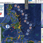
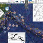
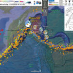
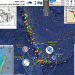
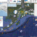
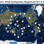
Here I summarize Earth’s significant seismicity for 2018. I limit this summary to earthquakes with magnitude greater than or equal to M 6.5. I am sure that there is a possibility that your favorite earthquake is not included in this review. Happy New Year.
However, our historic record is very short, so any thoughts about whether this year (or last, or next) has smaller (or larger) magnitude earthquakes than “normal” are limited by this small data set.
Here is a table of the earthquakes M ≥ 6.5.


Here is a plot showing the cumulative release of seismic energy. This summary is imperfect in several ways, but shows how only the largest earthquakes have a significant impact on the tally of energy release from earthquakes. I only include earthquakes M ≥ 6.5. Note how the M 7.5 Sulawesi earthquake and how little energy was released relative to the two M = 7.9 earthquakes.

Below is my summary poster for this earthquake year

  • I include moment tensors for the earthquakes included in the reports below.
  • Click on the map to see a larger version.


This is a video that shuffles through the earthquake report posters of the year


2018 Earthquake Report Pages

Other Annual Summaries

2018 Earthquake Reports

    General Overview of how to interact with these summaries

    • Click on the earthquake “magnitude and location” label (e.g. “M 6.9 Fiji”) to go to the Earthquake Report website for any given earthquake. Click on the map to open a high resolution pdf version of the interpretive poster. More information about the poster is found on the Earthquake Report website.
    • I plot the seismicity from the past month, with color representing depth and diameter representing magnitude (see legend). I include earthquake epicenters from 1918-2018 with magnitudes M ≥ 7.5 in one version.
    • I plot the USGS fault plane solutions (moment tensors in blue and focal mechanisms in orange), possibly in addition to some relevant historic earthquakes.

    Background on the Earthquake Report posters

    • I placed a moment tensor / focal mechanism legend on the posters. There is more material from the USGS web sites about moment tensors and focal mechanisms (the beach ball symbols). Both moment tensors and focal mechanisms are solutions to seismologic data that reveal two possible interpretations for fault orientation and sense of motion. One must use other information, like the regional tectonics, to interpret which of the two possibilities is more likely.
    • I also include the shaking intensity contours on the maps. These use the Modified Mercalli Intensity Scale (MMI; see the legend on the map). This is based upon a computer model estimate of ground motions, different from the “Did You Feel It?” estimate of ground motions that is actually based on real observations. The MMI is a qualitative measure of shaking intensity. More on the MMI scale can be found here and here. This is based upon a computer model estimate of ground motions, different from the “Did You Feel It?” estimate of ground motions that is actually based on real observations.
    • I include the slab 2.0 contours plotted (Hayes, 2018), which are contours that represent the depth to the subduction zone fault. These are mostly based upon seismicity. The depths of the earthquakes have considerable error and do not all occur along the subduction zone faults, so these slab contours are simply the best estimate for the location of the fault.li>

    Magnetic Anomalies

    • In the maps below, I include a transparent overlay of the magnetic anomaly data from EMAG2 (Meyer et al., 2017). As oceanic crust is formed, it inherits the magnetic field at the time. At different points through time, the magnetic polarity (north vs. south) flips, the north pole becomes the south pole. These changes in polarity can be seen when measuring the magnetic field above oceanic plates. This is one of the fundamental evidences for plate spreading at oceanic spreading ridges (like the Gorda rise).
    • Regions with magnetic fields aligned like today’s magnetic polarity are colored red in the EMAG2 data, while reversed polarity regions are colored blue. Regions of intermediate magnetic field are colored light purple.

2018.01.10 M 7.6 Cayman Trough

Just a couple hours ago there was an earthquake along the Swan fault, which is the transform plate boundary between the North America and Caribbean plates. The Cayman trough (CT) is a region of oceanic crust, formed at the Mid-Cayman Rise (MCR) oceanic spreading center. To the west of the MCR the CT is bound by the left-lateral strike-slip Swan fault. To the east of the MCR, the CT is bound on the north by the Oriente fault.
Based upon our knowledge of the plate tectonics of this region, I can interpret the fault plane solution for this earthquake. The M 7.6 earthquake was most likely a left-lateral strike-slip earthquake associated with the Swan fault.

  • Plotted with a century’s earthquakes with magnitudes M ≥ 6.5

  • Plotted with a century’s earthquakes with magnitudes M ≥ 3.5

  • There were two observations of a small amplitude (small wave height) tsunami recorded on tide gages in the region. Below are those observations.

2018.01.14 M 7.1 Peru

We had a damaging and (sadly) deadly earthquake in southern Peru in the last 24 hours. This is an earthquake, with magnitude M 7.1, that is associated with the subduction zone forming the Peru-Chile trench (PCT). The Nazca plate (NP) is subducting beneath the South America plate (SAP). There are lots of geologic structures on the Nazca plate that tend to affect how the subduction zone responds during earthquakes (e.g. segmentation).
In the region of this M 7.1 earthquake, two large structures in the NP are the Nazca Ridge and the Nazca fracture zone. The Nazca fracture zone is a (probably inactive) strike-slip fault system. The Nazca Ridge is an over-thickened region of the NP, thickened as the NP moved over a hotspot located near Salas y Gomez in the Pacific Ocean east of Easter Island (Ray et al., 2012).
There are many papers that discuss how the ridge affects the shape of the megathrust fault here. The main take-away is that the NR is bull dozing into South America and the dip of the subduction zone is flat here. There is a figure below that shows the deviation of the subducting slab contours at the NR.


Well, I missed looking further into a key update paper and used figures from an older paper on my interpretive poster yesterday. Thanks to Stéphane Baize for pointing this out! Turns out, after their new analyses, the M 7.1 earthquake was in a region of higher seismogenic coupling, rather than low coupling (as was presented in my first poster).
Also, Dr. Robin Lacassin noticed (as did I) the paucity of aftershocks from yesterday’s M 7.1. This was also the case for the carbon copy 2013 M 7.1 earthquake (there was 1 M 4.6 aftershock in the weeks following the M 7.1 earthquake on 2013.09.25; there were a dozen M 1-2 earthquakes in Nov. and Dec. of 2013, but I am not sure how related they are to the M 7.1 then). I present a poster below with this in mind. I also include below a comparison of the MMI modeled estimates. The 2013 seems to have possibly generated more widespread intensities, even though that was a deeper earthquake.

2018.01.23 M 7.9 Gulf of Alaska

  • 2018.01.23 M 7.9 Gulf of Alaska UPDATE #1
  • 2018.01.24 M 7.9 Gulf of Alaska UPDATE #2
  • This earthquake appears to be located along a reactivated fracture zone in the GA. There have only been a couple earthquakes in this region in the past century, one an M 6.0 to the east (though this M 6.0 was a thrust earthquake). The Gulf of Alaska shear zone is even further to the east and has a more active historic fault history (a pair of earthquakes in 1987-1988). The magnetic anomalies (formed when the Earth’s magnetic polarity flips) reflect a ~north-south oriented spreading ridge (the anomalies are oriented north-south in the region of today’s earthquake). There is a right-lateral offset of these magnetic anomalies located near the M 7.9 epicenter. Interesting that this right-lateral strike-slip fault (?) is also located at the intersection of the Gulf of Alaska shear zone and the 1988 M 7.8 earthquake (probably just a coincidence?). However, the 1988 M 7.8 earthquake fault plane solution can be interpreted for both fault planes (it is probably on the GA shear zone, but I don’t think that we can really tell).
    This is strange because the USGS fault plane is oriented east-west, leading us to interpret the fault plane solution (moment tensor or focal mechanism) as a left-lateral strike-slip earthquake. So, maybe this earthquake is a little more complicated than first presumed. The USGS fault model is constrained by seismic waves, so this is probably the correct fault (east-west).
    I prepared an Earthquake Report for the 1964 Good Friday Earthquake here.

    • The USGS updated their MMI contours to reflect their fault model. Below is my updated poster. I also added green dashed lines for the fracture zones related to today’s M 7.9 earthquake (on the magnetic anomaly inset map).

    • These are the observations as reported by the NTWC this morning (at 4:15 AM my local time).

    • Large Scale Interpretive Map (from update report)

    As a reminder, if the M 7.9 earthquake fault is E-W oriented, it would be left-lateral. The offset magnetic anomalies show right-lateral offset across these fracture zones. This was perhaps the main reason why I thought that the main fault was not E-W, but N-S. After a day’s worth of aftershocks, the seismicity may reveal some north-south trends. But, as a drama student in 7th grade (1977), my drama teacher (Ms. Naichbor, rest in peace) asked our class to go stand up on stage. We all stood in a line and she mentioned that this is social behavior, that people tend to stand in lines (and to avoid doing this while on stage). Later, when in college, professors often commented about how people tend to seek linear trends in data (lines). I actually see 3-4 N-S trends and ~2 E-W trends in the seismicity data.
    So, that being said, here is the animation I put together. I used the USGS query tool to get earthquakes from 1/22 until now, M ≥ 1.5. I include a couple inset maps presented in my interpretive posters. The music is copyright free. The animations run through twice.
    Here is a screenshot of the 14 MB video embedded below. I encourage you to view it in full screen mode (or download it).


    2018.02.16 M 7.2 Oaxaca, Mexico

    There was just now an earthquake in Oaxaca, Mexico between the other large earthquakes from last 2017.09.08 (M 8.1) and 2017.09.08 (M 7.1). There has already been a M 5.8 aftershock.Here is the USGS website for today’s M 7.2 earthquake.
    The SSN has a reported depth of 12 km, further supporting evidence that this earthquake was in the North America plate.
    This region of the subduction zone dips at a very shallow angle (flat and almost horizontal).
    There was also a sequence of earthquakes offshore of Guatemala in June, which could possibly be related to the M 8.1 earthquake. Here is my earthquake report for the Guatemala earthquake.
    The poster also shows the seismicity associated with the M 7.6 earthquake along the Swan fault (southern boundary of the Cayman trough). Here is my earthquake report for the Guatemala earthquake.

    • Here is the same poster but with the magnetic anomalies included (transparent).

    2018.02.25 M 7.5 Papua New Guinea

  • 2018.02.26 M 7.5 Papua New Guinea Update #1
  • This morning (local time in California) there was an earthquake in Papua New Guinea with, unfortunately, a high likelihood of having a good number of casualties. I was working on a project, so could not immediately begin work on this report.
    This M 7.5 earthquake (USGS website) occurred along the Papua Fold and Thrust Belt (PFTB), a (mostly) south vergent sequence of imbricate thrust faults and associated fold (anticlines). The history of this PFTB appears to be related to the collision of the Australia plate with the Caroline and Pacific plates, the delamination of the downgoing oceanic crust, and then associated magmatic effects (from decompression melting where the overriding slab (crust) was exposed to the mantle following the delamination). More about this can be found in Cloos et al. (2005).

  • The same map without historic seismicity.


  • The aftershocks are still coming in! We can use these aftershocks to define where the fault may have slipped during this M 7.5 earthquake. As I mentioned yesterday in the original report, it turns out the fault dimension matches pretty well with empirical relations between fault length and magnitude from Wells and Coppersmith (1994).
    The mapped faults in the region, as well as interpreted seismic lines, show an imbricate fold and thrust belt that dominates the geomorphology here (as well as some volcanoes, which are probably related to the slab gap produced by crust delamination; see Cloos et al., 2005 for more on this). I found a fault data set and include this in the aftershock update interpretive poster (from the Coordinating Committee for Geoscience Programmes in East and Southeast Asia, CCOP).
    I initially thought that this M 7.5 earthquake was on a fault in the Papuan Fold and Thrust Belt (PFTB). Mark Allen pointed out on twitter that the ~35km hypocentral depth is probably too deep to be on one of these “thin skinned” faults (see Social Media below). Abers and McCaffrey (1988) used focal mechanism data to hypothesize that there are deeper crustal faults that are also capable of generating the earthquakes in this region. So, I now align myself with this hypothesis (that the M 7.5 slipped on a crustal fault, beneath the thin skin deformation associated with the PFTB. (thanks Mark! I had downloaded the Abers paper but had not digested it fully.

    • Here is the “update” map with aftershocks

    2018.03.08 M 6.8 New Ireland

    We had an M 6.8 earthquake near a transform micro-plate boundary fault system north of New Ireland, Papua New Guinea today. Here is the USGS website for this earthquake.
    The main transform fault (Weitin fault) is ~40 km to the west of the USGS epicenter. There was a very similar earthquake on 1982.08.12 (USGS website).
    This earthquake is unrelated to the sequence occurring on the island of New Guinea.
    Something that I rediscovered is that there were two M 8 earthquakes in 1971 in this region. This testifies that it is possible to have a Great earthquake (M ≥ 8) close in space and time relative to another Great earthquake. These earthquakes do not have USGS fault plane solutions, but I suspect that these are subduction zone earthquakes (based upon their depth).
    This transform system is capable of producing Great earthquakes too, as evidenced by the 2000.11.16 M 8.0 earthquake (USGS website). This is another example of two Great earthquakes (or almost 2 Great earthquakes, as the M 7.8 is not quite a Great earthquake) are related. It appears that the M 8.0 earthquake may have triggered teh M 7.8 earthquake about 3 months later (however at first glance, it seemed to me like the strike-slip earthquake might not increase the static coulomb stress on the subduction zone, but I have not spent more than half a minute thinking about this).

    Main Interpretive Poster with emag2


    Earthquakes M≥ 6.5 with emag2


    2018.03.26 M 6.6 New Britain

    The New Britain region is one of the more active regions in the world. See a list of earthquake reports for this region at the bottom of this page, above the reference list.
    Today’s M 6.6 earthquake happened close in proximity to a M 6.3 from 2 days ago and a M 5.6 from a couple weeks ago. The M 5.6 may be related (may have triggered these other earthquakes), but this region is so active, it might be difficult to distinguish the effects from different earthquakes. The M 5.6 is much deeper and looks like it was in the downgoing Solomon Sea plate. It is much more likely that the M 6.3 and M 6.6 are related (I interpret that the M 6.3 probably triggered the M 6.6, or that M 6.3 was a foreshock to the M 6.6, given they are close in depth). Both M 6.3 and M 6.6 are at depths close to the depth of the subducting slab (the megathrust fault depth) at this location. So, I interpret these to be subduction zone earthquakes.

    2018.03.26 M 6.9 New Britain

    Well, those earthquakes from earlier, one a foreshock to a later one, were foreshocks to an earthquake today! Here is my report from a couple days ago. The M 6.6 and M 6.3 straddle today’s earthquake and all have similar hypocentral depths.

    2018.04.02 M 6.8 Bolivia

    A couple days ago there was a deep focus earthquake in the downgoing Nazca plate deep beneath Bolivia. This earthquake has an hypocentral depth of 562 km (~350 miles).
    We are still unsure what causes an earthquake at such great a depth. The majority of earthquakes happen at shallower depths, caused largely by the frictional between differently moving plates or crustal blocks (where earth materials like the crust behave with brittle behavior and not elastic behavior). Some of these shallow earthquakes are also due to internal deformation within plates or crustal blocks.
    As plates dive into the Earth at subduction zones, they undergo a variety of changes (temperature, pressure, stress). However, because people cannot directly observe what is happening at these depths, we must rely on inferences, laboratory analogs, and other indirect methods to estimate what is going on.
    So, we don’t really know what causes earthquakes at the depth of this Bolivia M 6.8 earthquake. Below is a review of possible explanations as provided by Thorne Lay (UC Santa Cruz) in an interview in response to the 2013 M 8.3 Okhotsk Earthquake.

    2018.05.04 M 6.9 Hawai’i

    There has been a swarm of earthquakes on the southeastern part of the big island, with USGS volcanologists hypothesizing about magma movement and suggesting that an eruption may be imminent. Here is a great place to find official USGS updates on the volcanism in Hawaii (including maps).
    Hawaii is an active volcanic island formed by hotspot volcanism. The Hawaii-Emperor Seamount Chain is a series of active and inactive volcanoes formed by this process and are in a line because the Pacific plate has been moving over the hotspot for many millions of years.
    Southeast of the main Kilauea vent, the Pu‘u ‘Ö‘ö crater saw an elevation of lava into the crater, leading to overtopping of the crater (on 4/30/2018). Seismicity migrated eastward along the ERZ. This morning, there was a M 5.0 earthquake in the region of the Hilina fault zone (HFZ). I was getting ready to write something up, but I had other work that I needed to complete. Then, this evening, there was a M 6.9 earthquake between the ERZ and the HFZ.
    There have been earthquakes this large in this region in the past (e.g. the 1975.1.29 M 7.1 earthquake along the HFZ). This earthquake was also most likely related to magma injection (Ando, 1979). The 1975 M 7.1 earthquake generated a small tsunami (Ando, 1979). These earthquakes are generally compressional in nature (including the earthquakes from today).
    Today’s earthquake also generated a tsunami as recorded on tide gages throughout Hawaii. There is probably no chance that a tsunami will travel across the Pacific to have a significant impact elsewhere.

    This version includes earthquakes M ≥ 3.5 (note the seismicity offshore to the south, this is where the youngest Hawaii volcano is).

    Below are a series of plots from tide gages installed at several sites in the Hawaii Island Chain. These data are all posted online here and here.

    • Hilo, Hawaii

    • Kawaihae, Hawaii

    Temblor Reports:

    • Click on the graphic to see a pdf version of the article.
    • Click on the html link (date) to visit the Temblor site.
    2018.05.05 Pele, the Hawai’i Goddess of Fire, Lightning, Wind, and Volcanoes
    2018.05.06 Pele, la Diosa Hawaiana del Fuego, los Relámpagos, el Viento y los Volcanes de Hawái

    2018.08.05 M 6.9 Lombok, Indonesia

    Yesterday morning, as I was recovering from working on stage crew for the 34th Reggae on the River (fundraiser for the non profit, the Mateel Community Center), I noticed on social media that there was an M 6.9 earthquake in Lombok, Indonesia. This is sad because of the likelihood for casualties and economic damage in this region.
    However, it is interesting because the earthquake sequence from last week (with a largest earthquake with a magnitude of M 6.4) were all foreshocks to this M 6.9. Now, technically, these were not really foreshocks. The M 6.4 has an hypocentral (3-D location) depth of ~6 km and the M 6.9 has an hypocentral depth of ~31 km. These earthquakes are not on the same fault, so I would interpret that the M 6.9 was triggered by the sequence from last week due to static coulomb changes in stress on the fault that ruptured. Given the large difference in depths, the uncertainty for these depths is probably not sufficient to state that they may be on the same fault (i.e. these depths are sufficiently different that this difference is larger than the uncertainty of their locations).
    I present a more comprehensive analysis of the tectonics of this region in my earthquake report for the M 6.4 earthquake here. I especially address the historic seismicity of the region there. This M 6.9 may have been on the Flores thrust system, while the earthquakes from last week were on the imbricate thrust faults overlying the Flores Thrust. See the map from Silver et al. (1986) below. I include the same maps as in my original report, but after those, I include the figures from Koulani et al. (2016) (the paper is available on researchgate).

    • Here is the map with a month’s seismicity plotted.

    2018.08.15 M 6.6 Aleutians

    Well, yesterday while I was installing the final window in a reconstruction project, there was an earthquake along the Aleutian Island Arc (a subduction zone) in the region of the Andreanof Islands. Here is the USGS website for the M 6.6 earthquake. This earthquake is close to the depth of the megathrust fault, but maybe not close enough. So, this may be on the subduction zone, but may also be on an upper plate fault (I interpret this due to the compressive earthquake fault mechanism). The earthquake has a hypocentral depth of 20 km and the slab model (see Hayes et al., 2013 below and in the poster) is at 40 km at this location. There is uncertainty in both the slab model and the hypocentral depth.
    The Andreanof Islands is one of the most active parts of the Aleutian Arc. There have been many historic earthquakes here, some of which have been tsunamigenic (in fact, the email that notified me of this earthquake was from the ITIC Tsunami Bulletin Board).
    Possibly the most significant earthquake was the 1957 Andreanof Islands M 8.6 Great (M ≥ 8.0) earthquake, though the 1986 M 8.0 Great earthquake is also quite significant. As was the 1996 M 7.9 and 2003 M 7.8 earthquakes. Lest we forget smaller earthquakes, like the 2007 M 7.2. So many earthquakes, so little time.

    • Here is the map with a month’s seismicity plotted.

    • Here is the map with a centuries seismicity plotted for earthquakes M ≥ 6.6.

    2018.08.18 M 8.2 Fiji

    We just had a Great Earthquake in the region of the Fiji Islands, in the central-western Pacific. Great Earthquakes are earthquakes with magnitudes M ≥ 8.0.
    This earthquake is one of the largest earthquakes recorded historically in this region. I include the other Large and Great Earthquakes in the posters below for some comparisons.
    Today’s earthquake has a Moment Magnitude of M = 8.2. The depth is over 550 km, so is very very deep. This region has an historic record of having deep earthquakes here. Here is the USGS website for this M 8.2 earthquake. While I was writing this, there was an M 6.8 deep earthquake to the northeast of the M 8.2. The M 6.8 is much shallower (about 420 km deep) and also a compressional earthquake, in contrast to the extensional M 8.2.
    This M 8.2 earthquake occurred along the Tonga subduction zone, which is a convergent plate boundary where the Pacific plate on the east subducts to the west, beneath the Australia plate. This subduction zone forms the Tonga trench.

    • Here is the map with a centuries seismicity plotted with M ≥ 7.5.

    2018.08.19 M 6.9 Lombok, Indonesia

    This ongoing sequence began in late July with a Mw 6.4 earthquake. Followed less than 2 weeks later with a Mw 6.9 earthquake.
    Today there was an M 6.3 soon followed by an M 6.9 earthquake (and a couple M 5.X quakes).
    These earthquakes have been occurring along a thrust fault system along the northern portion of Lombok, Indonesia, an island in the magamatic arc related to the Sunda subduction zone. The Flores thrust fault is a backthrust to the subduction zone. The tectonics are complicated in this region of the world and there are lots of varying views on the tectonic history. However, there has been several decades of work on the Flores thrust (e.g. Silver et al., 1986). The Flores thrust is an east-west striking (oriented) north vergent (dipping to the south) thrust fault that extends from eastern Java towards the Islands of Flores and Timor. Above the main thrust fault are a series of imbricate (overlapping) thrust faults. These imbricate thrust faults are shallower in depth than the main Flores thrust.
    The earthquakes that have been happening appear to be on these shallower thrust faults, but there is a possibility that they are activating the Flores thrust itself. Perhaps further research will illuminate the relations between these shallower faults and the main player, the Flores thrust.

    • Here is the map with a month’s seismicity plotted.

    • Here is an updated local scale (large scale) map showing the earthquake fault mechanisms for the current sequence. I label them with yellow numbers according to the sequence timing. I outlined the general areas that have had earthquakes into two zones (phases). Phase I includes the earthquakes up until today and Phase II includes the earthquakes from today. There is some overlap, but only for a few earthquakes. In general, it appears that the earthquakes have slipped in two areas of the Flores fault (or maybe two shallower thrust faults).

    • Here is the interpretive posted from the M 6.4 7/28 earthquake, with historic seismicity and earthquake mechanisms.

    2018.08.21 M 7.3 Venezuela

    We just had a M 7.3 earthquake in northern Venezuela. Sadly, this large earthquake has the potential to be quite damaging to people and their belongings (buildings, infrastructure).
    The northeastern part of Venezuela lies a large strike-slip plate boundary fault, the El Pilar fault. This fault is rather complicated as it strikes through the region. There are thrust faults and normal faults forming ocean basins and mountains along strike.
    Many of the earthquakes along this fault system are strike-slip earthquakes (e.g. the 1997.07.09 M 7.0 earthquake which is just to the southwest of today’s temblor. However, today’s earthquake broke my immediate expectations for strike-slip tectonics. There is a south vergent (dipping to the north) thrust fault system that strikes (is oriented) east-west along the Península de Paria, just north of highway 9, east of Carupano, Venezuela. Audenard et al. (2000, 2006) compiled a Quaternary Fault database for Venezuela, which helps us interpret today’s earthquake. I suspect that this earthquake occurred on this thrust fault system. I bet those that work in this area even know the name of this fault. However, looking at the epicenter and the location of the thrust fault, this is probably not on this thrust fault. When I initially wrote this report, the depth was much shallower. Currently, the hypocentral (3-D location) depth is 123 km, so cannot be on that thrust fault.
    The best alternative might be the subduction zone associated with the Lesser Antilles.

    • Here is the map with a month’s seismicity plotted, along with USGS earthquakes M ≥ 6.0.

    2018.08.24 M 7.1 Peru

    Well, this earthquake, while having a large magnitude, was quite deep. Because earthquake intensity decreases with distance from the earthquake source, the shaking intensity from this earthquake was so low that nobody submitted a single report to the USGS “Did You Feel It?” website for this earthquake.
    While doing my lit review, I found the Okal and Bina (1994) paper where they use various methods to determine focal mechanisms for the some deep earthquakes in northern Peru. More about focal mechanisms below. These authors created focal mechanisms for the 1921 and 1922 deep earthquakes so they could lean more about the 1970 deep earthquake. Their seminal work here forms an important record of deep earthquakes globally. These three earthquakes are all extensional earthquakes, similar to the other deep earthquakes in this region. I label the 1921 and 1922 earthquakes a couplet on the poster.
    There was also a pair of earthquakes that happened in November, 2015. These two earthquakes happened about 5 minutes apart. They have many similar characteristics, suggest that they slipped similar faults, if not the same fault. I label these as doublets also.
    So, there may be a doublet companion to today’s M 7.1 earthquake. However, there may be not. There are examples of both (single and doublet) and it might not really matter for 99.99% of the people on Earth since the seismic hazard from these deep earthquakes is very low.
    Other examples of doublets include the 2006 | 2007 Kuril Doublets (Ammon et al., 2008) and the 2011 Kermadec Doublets (Todd and Lay, 2013).

    • Here is the map with a century’s seismicity plotted, along with USGS earthquakes M ≥ 7.0.

    2018.09.05 M 6.6 Hokkaido, Japan

    Following the largest typhoon to strike Japan in a very long time, there was an earthquake on the island of Hokkaido, Japan today. There is lots on social media, including some spectacular views of disastrous and deadly landslides triggered by this earthquake (earthquakes are the number 1 source for triggering of landslides). These landslides may have been precipitated (sorry for the pun) by the saturation of hillslopes from the typhoon. Based upon the USGS PAGER estimate, this earthquake has the potential to cause significant economic damages, but hopefully a small number of casualties. As far as I know, this does not incorporate potential losses from earthquake triggered landslides [yet].
    This earthquake is in an interesting location. to the east of Hokkaido, there is a subduction zone trench formed by the subduction of the Pacific plate beneath the Okhotsk plate (on the north) and the Eurasia plate (to the south). This trench is called the Kuril Trench offshore and north of Hokkaido and the Japan Trench offshore of Honshu.
    One of the interesting things about this region is that there is a collision zone (a convergent plate boundary where two continental plates are colliding) that exists along the southern part of the island of Hokkaido. The Hidaka collision zone is oriented (strikes) in a northwest orientation as a result of northeast-southwest compression. Some suggest that this collision zone is no longer very active, however, there are an abundance of active crustal faults that are spatially coincident with the collision zone.
    Today’s M 6.6 earthquake is a thrust or reverse earthquake that responded to northeast-southwest compression, just like the Hidaka collision zone. However, the hypocentral (3-D) depth was about 33 km. This would place this earthquake deeper than what most of the active crustal faults might reach. The depth is also much shallower than where we think that the subduction zone megathrust fault is located at this location (the fault formed between the Pacific and the Okhotsk or Eurasia plates). Based upon the USGS Slab 1.0 model (Hayes et al., 2012), the slab (roughly the top of the Pacific plate) is between 80 and 100 km. So, the depth is too shallow for this hypothesis (Kuril Trench earthquake) and the orientation seems incorrect. Subduction zone earthquakes along the trench are oriented from northwest-southweast compression, a different orientation than today’s M 6.6.
    So today’s M 6.6 earthquake appears to have been on a fault deeper than the crustal faults, possibly along a deep fault associated with the collision zone. Though I am not really certain. This region is complicated (e.g. Kita et al., 2010), but there are some interpretations of the crust at this depth range (Iwasaki et al., 2004) shown in an interpreted cross section below.

    • Here is the map with a centuries seismicity plotted.

    Temblor Reports:

    • Click on the graphic to see a pdf version of the article.
    • Click on the html link (date) to visit the Temblor site.
    2018.09.06 Violent shaking triggers massive landslides in Sapporo Japan earthquake

    2018.09.09 M 6.9 Kermadec

    Today, there was a large earthquake associated with the subduction zone that forms the Kermadec Trench.
    This earthquake was quite deep, so was not expected to generate a significant tsunami (if one at all).
    There are several analogies to today’s earthquake. There was a M 7.4 earthquake in a similar location, but much deeper. These are an interesting comparison because the M 7.4 was compressional and the M 6.9 was extensional. There is some debate about what causes ultra deep earthquakes. The earthquakes that are deeper than about 40-50 km are not along subduction zone faults, but within the downgoing plate. This M 6.9 appears to be in a part of the plate that is bending (based on the Benz et al., 2011 cross section). As plates bend downwards, the upper part of the plate gets extended and the lower part of the plate experiences compression.

    • Here is the map with a month’s seismicity plotted.

    • Here is the map with a centuries seismicity plotted.

    2018.09.28 M 7.5 Sulawesi

  • 2018.10.16 M 7.5 Sulawesi UPDATE #1
  • Well, around 3 AM my time (northeastern Pacific, northern CA) there was a sequence of earthquakes including a mainshock with a magnitude M = 7.5. This earthquake happened in a highly populated region of Indonesia.
    This area of Indonesia is dominated by a left-lateral (sinistral) strike-slip plate boundary fault system. Sulawesi is bisected by the Palu-Kola / Matano fault system. These faults appear to be an extension of the Sorong fault, the sinistral strike-slip fault that cuts across the northern part of New Guinea.
    There have been a few earthquakes along the Palu-Kola fault system that help inform us about the sense of motion across this fault, but most have maximum magnitudes mid M 6.
    GPS and block modeling data suggest that the fault in this area has a slip rate of about 40 mm/yr (Socquet et al., 2006). However, analysis of offset stream channels provides evidence of a lower slip rate for the Holocene (last 12,000 years), a rate of about 35 mm/yr (Bellier et al., 2001). Given the short time period for GPS observations, the GPS rate may include postseismic motion earlier earthquakes, though these numbers are very close.
    Using empirical relations for historic earthquakes compiled by Wells and Coppersmith (1994), Socquet et al. (2016) suggest that the Palu-Koro fault system could produce a magnitude M 7 earthquake once per century. However, studies of prehistoric earthquakes along this fault system suggest that, over the past 2000 years, this fault produces a magnitude M 7-8 earthquake every 700 years (Bellier et al., 2006). So, it appears that this is the characteristic earthquake we might expect along this fault.
    Most commonly, we associate tsunamigenic earthquakes with subduction zones and thrust faults because these are the types of earthquakes most likely to deform the seafloor, causing the entire water column to be lifted up. Strike-slip earthquakes can generate tsunami if there is sufficient submarine topography that gets offset during the earthquake. Also, if a strike-slip earthquake triggers a landslide, this could cause a tsunami. We will need to wait until people take a deeper look into this before we can make any conclusions about the tsunami and what may have caused it.

    • There have been tsunami waves recorded on a tide gage over 300 km to the south of the epicenter, at a site called Mumuju. Below is a map and a plot of water surface elevations from this source.


    • Here is the map with a month’s seismicity plotted.

    • Here is the map with a centuries worth of seismicity plotted.

    Here is a map that shows the updated USGS model of ground shaking. The USGS prepared an updated earthquake fault slip model that was additionally informed by post-earthquake analysis of ground deformation. The original fault model extended from north of the epicenter to the northernmost extent of Palu City. Soon after the earthquake, Dr. Sotiris Valkaniotis prepared a map that showed large horizontal offsets across the ruptured fault along the entire length of the western margin on Palu Valley. This horizontal offset had an estimated ~8 meters of relative displacement. InSAR analyses confirmed that the coseismic ground deformation extended through Palu Valley and into the mountains to the south of the valley.

    My 2018.10.01 BC Newshour Interview

    InSAR Analysis

    Synthetic Aperture Radar (SAR) is a remote sensing method that uses Radar to make observations of Earth. These observations include the position of the ground surface, along with other information about the material properties of the Earth’s surface.
    Interferometric SAR (InSAR) utilizes two separate SAR data sets to determine if the ground surface has changed over time, the time between when these 2 data sets were collected. More about InSAR can be found here and here. Explaining the details about how these data are analyzed is beyond the scope of this report. I rely heavily on the expertise of those who do this type of analysis, for example Dr. Eric Fielding.

    • I prepared a map using the NASA-JPL InSAR data. They post all their data online here. I used the tiff image as it is georeferenced. However, some may prefer to use the kmz file in Google Earth.
    • I include the faults mapped by Wilkinson and Hall (2017), the PGA contours from the USGS model results. More on Peak Ground Acceleration (PGA) can be found here. I also include the spatial extent of the largest landslides that I mapped using post-earthquake satellite imagery provided by Digital Globe using their open source imagery program.


    M 7.5 Landslide Model vs. Observation Comparison

    Landslides during and following the M=7.5 earthquake in central Sulawesi, Indonesia possibly caused the majority of casualties from this catastrophic natural disaster. Volunteers (citizen scientists) have used satellite aerial imagery collected after the earthquake to document the spatial extent and magnitude of damage caused by the earthquake, landslides, and tsunami.
    Until these landslides are analyzed and compared with regions that did not fail in slope failure, we will not be able to reconstruct what happened… why some areas failed and some did not.
    There are landslide slope stability and liquefaction susceptibility models based on empirical data from past earthquakes. The USGS has recently incorporated these types of analyses into their earthquake event pages. More about these USGS models can be found on this page.
    I prepared some maps that compare the USGS landslide and liquefaction probability maps. Below I present these results along with the MMI contours. I also include the faults mapped by Wilkinson and Hall (2017). Shown are the cities of Donggala and Palu. Also shown are the 2 tide gage locations (Pantoloan Port – PP and Mumuju – M). I also used post-earthquake satellite imagery to outline the largest landslides in Palu Valley, ones that appear to be lateral spreads.

    • Here is the landslide probability map (Jessee et al., 2018). Below the poster I include the text from the USGS website that describes how this model is prepared.


    Nowicki Jessee and others (2018) is the preferred model for earthquake-triggered landslide hazard. Our primary landslide model is the empirical model of Nowicki Jessee and others (2018). The model was developed by relating 23 inventories of landslides triggered by past earthquakes with different combinations of predictor variables using logistic regression. The output resolution is ~250 m. The model inputs are described below. More details about the model can be found in the original publication. We modify the published model by excluding areas with slopes <5° and changing the coefficient for the lithology layer "unconsolidated sediments" from -3.22 to -1.36, the coefficient for "mixed sedimentary rocks" to better reflect that this unit is expected to be weak (more negative coefficient indicates stronger rock).To exclude areas of insignificantly small probabilities in the computation of aggregate statistics for this model, we use a probability threshold of 0.002.

    • Here is the liquefaction probability (susceptibility) map (Zhu et al., 2017). Note that the regions of low slopes in the valleys and coastal plains are the areas with a high chance of experiencing liquefaction. Areas of slopes >5° are excluded from this analysis.
    • Note that the large landslides (yellow polygons) are not in regions of high probability for liquefaction.


    Zhu and others (2017) is the preferred model for liquefaction hazard. The model was developed by relating 27 inventories of liquefaction triggered by past earthquakes to globally-available geospatial proxies (summarized below) using logistic regression. We have implemented the global version of the model and have added additional modifications proposed by Baise and Rashidian (2017), including a peak ground acceleration (PGA) threshold of 0.1 g and linear interpolation of the input layers. We also exclude areas with slopes >5°. We linearly interpolate the original input layers of ~1 km resolution to 500 m resolution. The model inputs are described below. More details about the model can be found in the original publication.

    Temblor Reports:

    • Click on the graphic to see a pdf version of the article.
    • Click on the html link (date) to visit the Temblor site.
    2018.09.28 The Palu-Koro fault ruptures in a M=7.5 quake in Sulawesi, Indonesia, triggering a tsunami and likely more shocks
    2018.10.03 Tsunami in Sulawesi, Indonesia, triggered by earthquake, landslide, or both
    2018.10.16 Coseismic Landslides in Sulawesi, Indonesia

    2018.10.10 M 7.0 New Britain, PNG

    In this region of the world, the Solomon Sea plate and the South Bismarck plate converge to form a subduction zone, where the Solomon Sea plate is the oceanic crust diving beneath the S.Bismarck plate.
    The subduction zone forms the New Britain Trench with an axis that trends east-northeast. To the east of New Britain, the subduction zone bends to the southeast to form the San Cristobal and South Solomon trenches. Between these two subduction zones is a series of oceanic spreading ridges sequentially offset by transform (strike slip) faults.
    Earthquakes along the megathrust at the New Britain trench are oriented with the maximum compressive stress oriented north-northwest (perpendicular to the trench). Likewise, the subduction zone megathrust earthquakes along the S. Solomon trench compress in a northeasterly direction (perpendicular to that trench).
    There is also a great strike slip earthquake that shows that the transform faults are active.
    This earthquake was too small and too deep to generate a tsunami.

    • Here is the map with a century’s seismicity plotted.

    Temblor Reports:

    • Click on the graphic to see a pdf version of the article.
    • Click on the html link (date) to visit the Temblor site.
    2018.10.10 M 7.5 Earthquake in New Britain, Papua New Guinea

    2018.10.22 M 6.8 Explorer plate

    This region of the Pacific-North America plate boundary is at the northern end of the Cascadia subduction zone (CSZ). To the east, the Explorer and Juan de Fuca plates subduct beneath the North America plate to form the megathrust subduction zone fault capable of producing earthquakes in the magnitude M = 9 range. The last CSZ earthquake was in January of 1700, just almost 319 years ago.
    The Juan de Fuca plate is created at an oceanic spreading center called the Juan de Fuca Ridge. This spreading ridge is offset by several transform (strike-slip) faults. At the southern terminus of the JDF Ridge is the Blanco fault, a transtensional transform fault connecting the JDF and Gorda ridges.
    At the northern terminus of the JDF Ridge is the Sovanco transform fault that strikes to the northwest of the JDF Ridge. There are additional fracture zones parallel and south of the Sovanco fault, called the Heck, Heckle, and Springfield fracture zones.
    The first earthquake (M = 6.6) appears to have slipped along the Sovanco fault as a right-lateral strike-slip earthquake. Then the M 6.8 earthquake happened and, given the uncertainty of the location for this event, occurred on a fault sub-parallel to the Sovanco fault. Then the M 6.5 earthquake hit, back on the Sovanco fault.

    • Here is the map with a century’s seismicity plotted.

    2018.10.25 M 6.8 Greece

    Before I looked more closely, I thought this sequence might be related to the Kefallonia fault. I prepared some earthquake reports for earthquakes here in the past, in 2015 and in 2016.
    Both of those earthquakes were right-lateral strike-slip earthquakes associated with the Kefallonia fault.
    However, today’s earthquake sequence was further to the south and east of the strike-slip fault, in a region experiencing compression from the Ionian Trench subduction zone. But there is some overlap of these different plate boundaries, so the M 6.8 mainshock is an oblique earthquake (compressional and strike-slip). Based upon the sequence, I interpret this earthquake to be right-lateral oblique. I could be wrong.

    • Here is the map with a century’s seismicity plotted.

    • Here is the tide gage data from Katakolo, which is only 65 km from the M 6.8 epicenter.

    Temblor Reports:

    • Click on the graphic to see a pdf version of the article.
    • Click on the html link (date) to visit the Temblor site.
    2018.10.26 Greek earthquake in a region of high seismic hazard

    2018.11.08 M 6.8 Mid Atlantic Ridge (Jan Mayen fracture zone)

    There was a M = 6.8 earthquake along a transform fault connecting segments of the Mid Atlantic Ridge recently.
    North of Iceland, the MAR is offset by many small and several large transform faults. The largest transform fault north of Iceland is called the Jan Mayen fracture zone, which is the location for the 2018.11.08 M = 6.8 earthquake.

    • Here is the map with a century’s seismicity plotted.

    • Here is the large scale map showing earthquake mechanisms for historic earthquakes in the region. Note how they mostly behave well (are almost perfectly aligned with the Jan Mayen fracture zone). There are a few exceptions, including an extensional earthquake possibly associated with extension on the MAR (2010.06.03 M = 5.6). Also, 2 earthquakes (2003.06.19 and 2005.07.25) are show oblique slip (not pure strike-slip as they have an amount of compressional motion) near the intersection of the fracture zone and the MAR.

    2018.11.30 M 7.0 Alaska

    Today’s earthquake occurred along the convergent plate boundary in southern Alaska. This subduction zone fault is famous for the 1964 March 27 M = 9.2 megathrust earthquake. I describe this earthquake in more detail here.
    During the 1964 earthquake, the downgoing Pacific plate slipped past the North America plate, including slip on “splay faults” (like the Patton fault, no relation, heheh). There was deformation along the seafloor that caused a transoceanic tsunami.
    The Pacific plate has pre-existing zones of weakness related to fracture zones and spreading ridges where the plate formed and are offset. There was an earthquake in January 2016 that may have reactivated one of these fracture zones. This earthquake (M = 7.1) was very deep (~130 km), but still caused widespread damage.
    The earthquake appears to have a depth of ~40 km and the USGS model for the megathrust fault (slab 2.0) shows the megathrust to be shallower than this earthquake. There are generally 2 ways that may explain the extensional earthquake: slab tension (the downgoing plate is pulling down on the slab, causing extension) or “bending moment” extension (as the plate bends downward, the top of the plate stretches out.

  • Temblor Report
    • Here is the map with a century’s seismicity plotted.

    Temblor Reports:

    • Click on the graphic to see a pdf version of the article.
    • Click on the html link (date) to visit the Temblor site.
    2018.11.30 Exotic M=7.0 earthquake strikes beneath Anchorage, Alaska
    2018.12.11 What the Anchorage earthquake means for the Bay Area, Southern California, Seattle, and Salt Lake City

    2018.12.05 M 7.5 New Caledonia

    There was a sequence of earthquakes along the subduction zone near New Caledonia and the Loyalty Islands.
    This part of the plate boundary is quite active and I have a number of earthquake reports from the past few years (see below, a list of earthquake reports for this region).
    But the cool thing from a plate tectonics perspective is that there was a series of different types of earthquakes. At first view, it appears that there was a mainshock with a magnitude of M = 7.5. There was a preceding M 6.0 earthquake which may have been a foreshock.
    The M 7.5 earthquake was an extensional earthquake. This may be due to either extension from slab pull or due to extension from bending of the plate. More on this later.
    Following the M 7.5, there was an M 6.6 earthquake, however, this was a thrust or reverse (compressional) earthquake. The M 6.6 may have been in the upper plate or along the subduction zone megathrust fault, but we won’t know until the earthquake locations are better determined.
    A similar sequence happened in October/November 2017. I prepared two reports for this sequence here and here. Albeit, in 2017, the thrust earthquake was first (2017.10.31 vs. 2017.11.19).
    There have been some observations of tsunami. Below is from the Pacific Tsunami Warning Center.

    • Here is the map with a month’s seismicity plotted.

    • Here is the map with a century’s seismicity plotted.

    2018.12.20 M 7.4 Bering Kresla

  • 2018.12.20 M 7.3 Bering Kresla UPDATE #1
  • A large earthquake in the region of the Bering Kresla fracture zone, a strike-slip fault system that coincides with the westernmost portion of the Aleutian trench (which is a subduction zone further to the east).
    This earthquake happened in an interesting region of the world where there is a junction between two plate boundaries, the Kamchatka subduction zone with the Aleutian subduction zone / Bering-Kresla Shear Zone. The Kamchatka Trench (KT) is formed by the subduction (a convergent plate boundary) beneath the Okhotsk plate (part of North America). The Aleutian Trench (AT) and Bering-Kresla Shear Zone (BKSZ) are formed by the oblique subduction of the Pacific plate beneath the Pacific plate. There is a deflection in the Kamchatka subduction zone north of the BKSZ, where the subduction trench is offset to the west. Some papers suggest the subduction zone to the north is a fossil (inactive) plate boundary fault system. There are also several strike-slip faults subparallel to the BKSZ to the north of the BKSZ.

    • Here is the map with a month’s seismicity plotted, including the age of the crust.

    • Here is the map with a century’s seismicity plotted, with earthquakes M ≥ 6.0, including the age of the crust.

    UPDATE #1

    • Here is the map with a month’s seismicity plotted.

    • Here is the map with a century’s seismicity plotted, with earthquakes M ≥ 6.0.

    2018.12.29 M 7.0 Philippines

    This magnitude M = 7.0 earthquake is related to the subduction zone that forms the Philippine trench (where the Philippine Sea plate subducts beneath the Sunda plate). Here is the USGS website for this earthquake.
    The earthquake was quite deep, which makes it less likely to cause damage to people and their belongings (e.g. houses and roads) and also less likely that the earthquake will trigger a trans-oceanic tsunami.
    Here are the tidal data:

    • Here is the map with a century’s seismicity plotted.

    Geologic Fundamentals

    • For more on the graphical representation of moment tensors and focal mechnisms, check this IRIS video out:
    • Here is a fantastic infographic from Frisch et al. (2011). This figure shows some examples of earthquakes in different plate tectonic settings, and what their fault plane solutions are. There is a cross section showing these focal mechanisms for a thrust or reverse earthquake. The upper right corner includes my favorite figure of all time. This shows the first motion (up or down) for each of the four quadrants. This figure also shows how the amplitude of the seismic waves are greatest (generally) in the middle of the quadrant and decrease to zero at the nodal planes (the boundary of each quadrant).

    • Here is another way to look at these beach balls.
    • There are three types of earthquakes, strike-slip, compressional (reverse or thrust, depending upon the dip of the fault), and extensional (normal). Here is are some animations of these three types of earthquake faults. The following three animations are from IRIS.
    • Strike Slip:

      Compressional:

      Extensional:

    • This is an image from the USGS that shows how, when an oceanic plate moves over a hotspot, the volcanoes formed over the hotspot form a series of volcanoes that increase in age in the direction of plate motion. The presumption is that the hotspot is stable and stays in one location. Torsvik et al. (2017) use various methods to evaluate why this is a false presumption for the Hawaii Hotspot.

    • A cutaway view along the Hawaiian island chain showing the inferred mantle plume that has fed the Hawaiian hot spot on the overriding Pacific Plate. The geologic ages of the oldest volcano on each island (Ma = millions of years ago) are progressively older to the northwest, consistent with the hot spot model for the origin of the Hawaiian Ridge-Emperor Seamount Chain. (Modified from image of Joel E. Robinson, USGS, in “This Dynamic Planet” map of Simkin and others, 2006.)

    • Here is a map from Torsvik et al. (2017) that shows the age of volcanic rocks at different locations along the Hawaii-Emperor Seamount Chain.

    • Hawaiian-Emperor Chain. White dots are the locations of radiometrically dated seamounts, atolls and islands, based on compilations of Doubrovine et al. and O’Connor et al. Features encircled with larger white circles are discussed in the text and Fig. 2. Marine gravity anomaly map is from Sandwell and Smith.

    Return to the Earthquake Reports page.

    Earthquake Report: Philippines

    Earlier there was an earthquake in the Philippines. This magnitude M = 7.0 earthquake is related to the subduction zone that forms the Philippine trench (where the Philippine Sea plate subducts beneath the Sunda plate). Here is the USGS website for this earthquake.
    The earthquake was quite deep, which makes it less likely to cause damage to people and their belongings (e.g. houses and roads) and also less likely that the earthquake will trigger a trans-oceanic tsunami. There may be a small tsunami in the region, but this is also not very likely.
    There have been many large earthquakes in this part of the subduction zone in the 20th and 21st centuries. Based on the historic pattern, it is possible that there may be another earthquake of similar magnitude in the near to distant future (within a year or two). It is also possible that there may be a larger magnitude earthquake.
    Look at the pair of earthquakes that occurred on 17 May 2017. The M = 7.1 earthquake preceded the M = 7.3 earthquake by less than an hour. While, the 1995.05.05 M = 7.1 and 1996.06.11 M = 7.1 earthquakes happened about a year from each other.
    There may have been a small tsunami at Lahad Datu, Sabah (~1,000 km to the west of the earthquake, shown as a yellow square on the poster below). The earthquake happened at about 03:39:09 (UTC) and the plot below uses this same time reference. The wave begins at around 05:00. A rough estimate using the shallow water equation and an average water depth (Celebes Sea) suggests that the wave might have traveled 712 km/hr (so this 5:00 arrival appears close to the time it might take to get there).
    Here are the tidal data:

    Below is my interpretive poster for this earthquake

    I plot the seismicity from the past month, with color representing depth and diameter representing magnitude (see legend). I include earthquake epicenters from 1918-2018 with magnitudes M ≥ 7.0 in one version.
    I plot the USGS fault plane solutions (moment tensors in blue and focal mechanisms in orange), possibly in addition to some relevant historic earthquakes.

    • I placed a moment tensor / focal mechanism legend on the poster. There is more material from the USGS web sites about moment tensors and focal mechanisms (the beach ball symbols). Both moment tensors and focal mechanisms are solutions to seismologic data that reveal two possible interpretations for fault orientation and sense of motion. One must use other information, like the regional tectonics, to interpret which of the two possibilities is more likely.
    • I also include the shaking intensity contours on the map. These use the Modified Mercalli Intensity Scale (MMI; see the legend on the map). This is based upon a computer model estimate of ground motions, different from the “Did You Feel It?” estimate of ground motions that is actually based on real observations. The MMI is a qualitative measure of shaking intensity. More on the MMI scale can be found here and here. This is based upon a computer model estimate of ground motions, different from the “Did You Feel It?” estimate of ground motions that is actually based on real observations.
    • I include the slab 2.0 contours plotted (Hayes, 2018), which are contours that represent the depth to the subduction zone fault. These are mostly based upon seismicity. The depths of the earthquakes have considerable error and do not all occur along the subduction zone faults, so these slab contours are simply the best estimate for the location of the fault.li>

      I include some inset figures. Some of the same figures are located in different places on the larger scale map below.

    • In the lower left corner is a map from Smoczyk et al. (2013) that shows historic seismicity and the major plate boundaries. I place a blue star in the location of today’s M = 7.0 earthquake.
    • Above this map is a cross section showing seismicity associated with the downgoing Philippine sea plate. The location of this cross section D-D’ is shown on the main map as a cyan line. The 3-D location of the earthquake (hypocenter) is shown on the cross section also.
    • In the upper left corner is a figure from Hall, 2011. This shows the plate tectonic configuration in the equatorial Pacific. Note how the upper panel shows a west dipping slab on the east side of the Philippines. Note the contrast in the center panel (Halmahera), where the eastern fault is dipping to the east (westward vergent) and the western fault is dipping to the west (eastward vergent). This region near Halmahera forms the Molucca Strait, one of the most tectonically active areas in this region.
    • In the lower right corner is a seismic hazard map from Smoczyk et al. (2013) that shows how this region has a high seismic hazard.
    • In the upper right corner is the seismic hazard map from Temblor.net. Temblor.net uses the Global Earth Activity Rate (GEAR) model to provide estimates of seismic hazard at a global to local scale (Bird et al., 2015). GEAR blends quakes during the past 41 years with strain of the Earth’s crust as measured using Global Positioning System (GPS) observations. The model shows that this M = 7.0 earthquake (the largest red dot) happened in a region that may experience an earthquake with a magnitude range of 7.75 < M < 8.0.
    • Here is the map with a month’s seismicity plotted.

    • Here is the map with a century’s seismicity plotted.

    Other Report Pages

    Some Relevant Discussion and Figures

    • Here is a map that shows a simplified version of the subduction zones in the region (Galgana et al., 2007).

    • Physical map of the Philippines, showing topography and bathymetry. The two opposing subduction zones (the Manila Trench and the Philippine Trench/East Luzon Trough), major plates (SUND and PHSP) and the major Philippine Fault System with splays in Luzon (yellow lines) are mapped (basemap derived from the UNAVCO Jules Verne Navigator).

    • This is the low-angle oblique view of the region (Hall, 2011).

    • 3D cartoon of plate boundaries in the Molucca Sea region modified from Hall et al. (1995). Although seismicity identifies a number of plates there are no continuous boundaries, and the Cotobato, North Sulawesi and Philippine Trenches are all intraplate features. The apparent distinction between different crust types, such as Australian continental crust and oceanic crust of the Philippine and Molucca Sea, is partly a boundary inactive since the Early Miocene (east Sulawesi) and partly a younger but now probably inactive boundary of the Sorong Fault. The upper crust of this entire region is deforming in a much more continuous way than suggested by this cartoon.

    • This is smaller scale tectonic map of the region (Zahirovic et al., 2014).

    • Regional tectonic setting with plate boundaries (MORs/transforms = black, subduction zones = teethed red) from Bird (2003) and ophiolite belts representing sutures modified from Hutchison (1975) and Baldwin et al. (2012). West Sulawesi basalts are from Polvé et al. (1997), fracture zones are from Matthews et al. (2011) and basin outlines are from Hearn et al. (2003). ANI – Andaman and Nicobar Islands, BD– Billiton Depression, Ba – Bangka Island, BI – Belitung (Billiton) Island, BiS – Bismarck Sea, BP – Benham Plateau, CaR – Caroline Ridge, CS – Celebes Sea, DG– Dangerous Grounds, EauR – Eauripik Ridge, FIN – Finisterre Terrane, GoT – Gulf of Thailand, GR– Gagua Ridge, HAL– Halmahera, HBa – Huatung Basin, KB–Ketungau Basin, KP – Khorat Platform, KT – Kiilsgaard Trough, LS – Luconia Shoals, MacB – Macclesfield Bank, ManTr – Manus Trench, MaTr – Mariana Trench, MB– Melawi Basin, MDB– Minami Daito Basin, MG– Mangkalihat, MIN – Mindoro, MN– Mawgyi Nappe, MoS – Molucca Sea, MS– Makassar Straits, MTr – Mussau Trench, NGTr – New Guinea Trench, NI – Natuna Islands, ODR– Oki Daito Ridge, OJP –Ontong Java Plateau, OSF – Owen Stanley Fault, PAL – Palawan, PhF – Philippine Fault, PT – Paternoster Platform, PTr – Palau Trench, PVB – Parece Vela Basin, RB – Reed Bank, RMF– Ramu-Markham Fault, RRF – Red River fault, SEM– Semitau, ShB – Shikoku Basin, Sol. Sea – Solomon Sea, SPK – Sepik, SPT – abah–Palawan Trough, STr – Sorol Trough, Sul – Sulawesi, SuS – Sulu Sea, TPAA– Torricelli–Prince Alexander Arc, WB–West Burma, WCT–W Caroline Trough, YTr –Yap Trough.

    • This is a map and series of cross sections showing subducting plates in blue (Zahirovic et al., 2014). The cross sections are based upon seismic wave tomography, which is similar to CT scans (Computed Tomography of X-Rays). These two processes use the same general methods to investigate the 3-dimensional views of internal structures (bodies vs. the Earth). More can be found in their paper, but basically, the blue regions represent areas that have higher seismic velocity. Oceanic lithosphere has higher seismic velocities than the surrounding mantle. So, the subducting oceanic slabs show up as blue. The corss section G-G’ is at about the same latitude as the M = 7.0 earthquake. Note that the Philippine sea plate subducting at the Philippine trench (dipping to the west/left) is evident, while the slab associated with the Cotobato trench does not appear visible. Compare this with the seismicity cross section from Smoczyck et al. (2013), where the Cotobato trench seismicity is much more shallow than the Philippine trench.

    • Vertical sections from MIT-P (Li et al., 2008) and GyPSuM-S (Simmons et al., 2009) seismic tomography models along profiles A to E (magenta lines). The first-order differences between the P- and S-wave models is that the amplitude of the positive seismic velocity anomalies significantly diminishes away from continental coverage (e.g., dashed lines in profiles A and B). A depth slice at 746 km from MIT-P isprovided for reference with super-imposed present-day coastlines and plate boundaries. Interpreted slab sources are labeled: GI-BA= Greater India–Neo-Tethyan back-arc slab, M/N-T – Meso- and Neo-Tethyan slabs, W-S –Woyla–Sunda slabs, S – Sunda slab, PSCS – proto-South China Sea slab, PAC – Pacific slab, PMOL– proto-Molucca slab, PSOL – proto-Solomon slab, CS – Caroline slab, PSP – Philippine Sea Plate slab, S-C = Sulu–Celebes slabs.

    • However, here is a figure that shows isosurfaces from their tomography models (Zahirovic et al., 2014). This shows what may be slabs related to the Cotobato trench (western part of G-G’ cross section). These slabs show up better on the lower figure.

    • 3-D visualization of +0.2% seismic velocity anomaly isosurfaces in MIT-P (top) and +0.9% seismic velocity perturbation in GyPSuM-S (bottom) models. Profiles A to G represent the vertical profiles (see Fig. 10) that capture the convergence and subduction histories of the region since the Cretaceous. Present-day coastlines are translucent grey shades, and present-day plate boundaries are translucent black lines. Slab volumes are colored by their depth, while the light blue color represents the interior surface of these slabs. PSCS – proto-South China Sea slab.

    • This map shows the seismic hazard for this region. The color represents the likelihood of any region experiencing ground shaking of a particular magnitude. The scale is “Peak Ground Acceleration.” Units are m/s^2. Purple represents gravitational acceleration of 1 g, gravity at Earth’s surface. Note how most of the earthquakes were in the region of higher likely ground shaking, except for the Sulawesi earthquakes.

    Geologic Fundamentals

    • For more on the graphical representation of moment tensors and focal mechnisms, check this IRIS video out:
    • Here is a fantastic infographic from Frisch et al. (2011). This figure shows some examples of earthquakes in different plate tectonic settings, and what their fault plane solutions are. There is a cross section showing these focal mechanisms for a thrust or reverse earthquake. The upper right corner includes my favorite figure of all time. This shows the first motion (up or down) for each of the four quadrants. This figure also shows how the amplitude of the seismic waves are greatest (generally) in the middle of the quadrant and decrease to zero at the nodal planes (the boundary of each quadrant).

    • Here is another way to look at these beach balls.
    • There are three types of earthquakes, strike-slip, compressional (reverse or thrust, depending upon the dip of the fault), and extensional (normal). Here is are some animations of these three types of earthquake faults. The following three animations are from IRIS.
    • Strike Slip:

      Compressional:

      Extensional:

    • This is an image from the USGS that shows how, when an oceanic plate moves over a hotspot, the volcanoes formed over the hotspot form a series of volcanoes that increase in age in the direction of plate motion. The presumption is that the hotspot is stable and stays in one location. Torsvik et al. (2017) use various methods to evaluate why this is a false presumption for the Hawaii Hotspot.

    • A cutaway view along the Hawaiian island chain showing the inferred mantle plume that has fed the Hawaiian hot spot on the overriding Pacific Plate. The geologic ages of the oldest volcano on each island (Ma = millions of years ago) are progressively older to the northwest, consistent with the hot spot model for the origin of the Hawaiian Ridge-Emperor Seamount Chain. (Modified from image of Joel E. Robinson, USGS, in “This Dynamic Planet” map of Simkin and others, 2006.)

    • Here is a map from Torsvik et al. (2017) that shows the age of volcanic rocks at different locations along the Hawaii-Emperor Seamount Chain.

    • Hawaiian-Emperor Chain. White dots are the locations of radiometrically dated seamounts, atolls and islands, based on compilations of Doubrovine et al. and O’Connor et al. Features encircled with larger white circles are discussed in the text and Fig. 2. Marine gravity anomaly map is from Sandwell and Smith.

      References:

    • Bird, P., Jackson, D. D., Kagan, Y. Y., Kreemer, C., and Stein, R. S., 2015. GEAR1: A global earthquake activity rate model constructed from geodetic strain rates and smoothed seismicity, Bull. Seismol. Soc. Am., v. 105, no. 5, p. 2538–2554, DOI: 10.1785/0120150058
    • Galgana, G., Hamburger, M., McCaffrey, R., Corpuz, E., and Chen, Q., 2007. Analysis of crustal deformation in Luzon, Philippines using geodetic observations and earthquake focal mechanisms in Tectonophysics, v. 432, p. 63-67., doi:10.1016/j.tecto.2006.12.001
    • Hall, R., 2011. Australia–SE Asia collision: plate tectonics and crustal flow in Hall, R., Cottam, M. A. &Wilson, M. E. J. (eds) The SE Asian Gateway: History and Tectonics of the Australia–Asia Collision. Geological Society, London, Special Publications, 355, 75–109.
    • Hayes, G., 2018, Slab2 – A Comprehensive Subduction Zone Geometry Model: U.S. Geological Survey data release, https://doi.org/10.5066/F7PV6JNV.
    • Noda, A., 2013. Strike-Slip Basin – Its Configuration and Sedimentary Facies in Mechanism of Sedimentary Basin Formation – Multidisciplinary Approach on Active Plate Margins http://www.intechopen.com/books/mechanism-of-sedimentarybasin-formation-multidisciplinary-approach-on-active-plate-margins http://dx.doi.org/10.5772/56593
    • Smoczyk, G.M., Hayes, G.P., Hamburger, M.W., Benz, H.M., Villaseñor, Antonio, and Furlong, K.P., 2013. Seismicity of the Earth 1900–2012 Philippine Sea plate and vicinity: U.S. Geological Survey Open-File Report 2010–1083-M, 1 sheet, scale 1:10,000,000.
    • Waltham et al., 2008. Basin formation by volcanic arc loading in GSA Special Papers 2008, v. 436, p. 11-26.
    • Zahirovic et al., 2014. The Cretaceous and Cenozoic tectonic evolution of Southeast Asia in Solid Earth, v. 5, p. 227-273, doi:10.5194/se-5-227-2014.

    Return to the Earthquake Reports page.


    Earthquake Report: Bering Kresla Update #1

    Well, the USGS updated their earthquake mechanism (moment tensor) to be more steeply dipping, showing a more vertical fault possibly. This makes more sense given the historic earthquakes in this region and our knowledge of the history of this complicated plate boundary. The USGS also updated their model of shaking intensity (MMI) and revised the magnitude to M =7.3 (though I keep M = 7.4 in these reports to avoid confusion).
    I present a larger scale map with more historic earthquake mechanisms below.
    These historic mechanisms reveal something about how the Pacific plate subducts beneath the Okhotsk plate (part of North America). Read more about the tectonics and my initial interpretation of this earthquake in the first earthquake report here.
    The M = 7.4 earthquake from yesterday clearly ruptured the Aleutian fracture zone (AFZ), which is part of the Bering Kresla Shear zone. There is a series of aftershocks that plot to the southwest of the mainshock, but these are mislocated. The M =7.4 was originally located to the southwest also (off of the fault), but has since been relocated. So, I suspect that these aftershocks could be relocated also, if someone were to work on them (e.g. double difference analysis). The 1978.03.03 M 6.2 earthquake is a great analogy for this M 7.4 as it is in the same location and has a nice right-lateral strike slip focal mechanism.
    The relative motion between the Pacific plate and North America plate here is parallel to the plate boundary, giving rise to this shear zone. To the west, the Pacific plate subducts beneath the Okhotsk plate to form the Kuril/Kamchatka trench.
    We can see strike slip earthquakes west of the trench (1984.11.01 and 1986.05.02). Further to the west, there are some earthquakes that show the convergence associated with this subduction margin (1983.01.09, 1982.11.21, 1997.12.05). The Aleutian fracture zone exists within the Pacific plate as it dives beneath the Okhotsk plate,as evidenced by the 2004.04.14 M = 6.2 earthquake.

    Below is my interpretive poster for this earthquake

    I plot the seismicity from the past month, with color representing depth and diameter representing magnitude (see legend). I include earthquake epicenters from 1918-2018 with magnitudes M ≥ 6.0 in one version.
    I plot the USGS fault plane solutions (moment tensors in blue and focal mechanisms in orange), possibly in addition to some relevant historic earthquakes.

    • I placed a moment tensor / focal mechanism legend on the poster. There is more material from the USGS web sites about moment tensors and focal mechanisms (the beach ball symbols). Both moment tensors and focal mechanisms are solutions to seismologic data that reveal two possible interpretations for fault orientation and sense of motion. One must use other information, like the regional tectonics, to interpret which of the two possibilities is more likely.
    • I also include the shaking intensity contours on the map. These use the Modified Mercalli Intensity Scale (MMI; see the legend on the map). This is based upon a computer model estimate of ground motions, different from the “Did You Feel It?” estimate of ground motions that is actually based on real observations. The MMI is a qualitative measure of shaking intensity. More on the MMI scale can be found here and here. This is based upon a computer model estimate of ground motions, different from the “Did You Feel It?” estimate of ground motions that is actually based on real observations.
    • I include the slab 2.0 contours plotted (Hayes, 2018), which are contours that represent the depth to the subduction zone fault. These are mostly based upon seismicity. The depths of the earthquakes have considerable error and do not all occur along the subduction zone faults, so these slab contours are simply the best estimate for the location of the fault.li>

      Magnetic Anomalies

    • In the map below, I include a transparent overlay of the magnetic anomaly data from EMAG2 (Meyer et al., 2017). As oceanic crust is formed, it inherits the magnetic field at the time. At different points through time, the magnetic polarity (north vs. south) flips, the north pole becomes the south pole. These changes in polarity can be seen when measuring the magnetic field above oceanic plates. This is one of the fundamental evidences for plate spreading at oceanic spreading ridges (like the Gorda rise).
    • Regions with magnetic fields aligned like today’s magnetic polarity are colored red in the EMAG2 data, while reversed polarity regions are colored blue. Regions of intermediate magnetic field are colored light purple.

      I include some inset figures. Some of the same figures are located in different places on the larger scale map below.

    • In the upper right corner I include a map that shows more details about the faulting in the region (Konstantinovskaia (2001).
    • In the upper left corner is a map from Gaedicke et a. (2000) that shows a detailed map of the faulting in the region. Note that there are strike-slip, normal, and thrust faults all overlapping in cool ways. When I wrote my intitial report, I hypothesized that the M = 7.4 earthquake was extensional and one of the reasons this may happen here is that there are normal faults (extensional) that form sedimentary basins in this area (e.g. the Steller Basin).
    • In the lower center, I present a cross section (seismic reflection data) showing the bathymetry from A-A’ (location shown on upper left map and the main map as a green bar bell line) from Gaedicke et al. (2000). Note the different fracture zones. I place a blue star in the general location of the M = 7.4 earthquake.
    • Here is the map with a month’s seismicity plotted.

    • Here is the map with a century’s seismicity plotted, with earthquakes M ≥ 6.0.

    Some Relevant Discussion and Figures

    • Here is the large scale map from Gaedicke et al. (2000). Note that the map in the poster is rotated so that north is up, because in this map, north is not “up.” Note the location of the cross sections A-A’ and B-B’.

    • Here are the two cross sections (seismic reflection) showing the topography created by these fracture zones (Gaedicke et al., 2000). The lower cross section shows a basin formed by the transtension (extension associated with a strike-slip fault) along the Bering fracture zone.

    • Here is the more detailed tectonic map from Konstantinovskaia et al. (2001).


    • This is the cross section associated with the above map, showing subduction at the Kuril/Kamchatka trench.


    • Below are a series of maps that show the tectonic history in the northwest Pacific. This helps us learn how the plate boundary of the westernmost Aleutian trench is very different from the history of the subduction zone further to the east (responsible for the 1964 Good Friday earthquake for example). The time series begins at the beginning of the Tertiary at about 65 million years ago.


    • Finally, here I present tide gage records from the IOC sea level monitoring website. The M = 7.4 earthquake occurred at 2018-12-20 17:01:55 (UTC) and these plots use the UTC time scale. We may observe that there were no tsunami recorded at these gages here and here.


    • However, if we take a look at some DART buoy data, we do see some perturbations. Dr. Lori Dengler (emeritus professor at the Humboldt State University, Department of Geology) suggests that these data show surface waves being recorded by these sensors. Below are plots from this buoy. The upper panel are the raw data and the lower panel are the data relative to the prediction.


    Geologic Fundamentals

    • For more on the graphical representation of moment tensors and focal mechnisms, check this IRIS video out:
    • Here is a fantastic infographic from Frisch et al. (2011). This figure shows some examples of earthquakes in different plate tectonic settings, and what their fault plane solutions are. There is a cross section showing these focal mechanisms for a thrust or reverse earthquake. The upper right corner includes my favorite figure of all time. This shows the first motion (up or down) for each of the four quadrants. This figure also shows how the amplitude of the seismic waves are greatest (generally) in the middle of the quadrant and decrease to zero at the nodal planes (the boundary of each quadrant).

    • Here is another way to look at these beach balls.
    • There are three types of earthquakes, strike-slip, compressional (reverse or thrust, depending upon the dip of the fault), and extensional (normal). Here is are some animations of these three types of earthquake faults. The following three animations are from IRIS.
    • Strike Slip:

      Compressional:

      Extensional:

    • This is an image from the USGS that shows how, when an oceanic plate moves over a hotspot, the volcanoes formed over the hotspot form a series of volcanoes that increase in age in the direction of plate motion. The presumption is that the hotspot is stable and stays in one location. Torsvik et al. (2017) use various methods to evaluate why this is a false presumption for the Hawaii Hotspot.

    • A cutaway view along the Hawaiian island chain showing the inferred mantle plume that has fed the Hawaiian hot spot on the overriding Pacific Plate. The geologic ages of the oldest volcano on each island (Ma = millions of years ago) are progressively older to the northwest, consistent with the hot spot model for the origin of the Hawaiian Ridge-Emperor Seamount Chain. (Modified from image of Joel E. Robinson, USGS, in “This Dynamic Planet” map of Simkin and others, 2006.)

    • Here is a map from Torsvik et al. (2017) that shows the age of volcanic rocks at different locations along the Hawaii-Emperor Seamount Chain.

    • Hawaiian-Emperor Chain. White dots are the locations of radiometrically dated seamounts, atolls and islands, based on compilations of Doubrovine et al. and O’Connor et al. Features encircled with larger white circles are discussed in the text and Fig. 2. Marine gravity anomaly map is from Sandwell and Smith.

      Social Media

      References:

    • Bindeman, I.N., Vinogradov, V.I., Valley, J.W., Wooden, J.L., and Natal’in, B.A., 2002. Archean Protolith and Accretion of Crust in Kamchatka: SHRIMP Dating of Zircons from Sredinny and Ganal Massifs in The Journal of Geology, v. 110, p. 271-289.
    • Gaedicke, C., Baranov, B., Seliverstov, N., Alexeiev, D., Tsdukanaov, N., and Freitag, R., 2000. Structure of an active arc-continent collision area: the Aleutian–Kamchatka junction in Tecrtonophysics, v. 325, p. 63-85.
    • Hayes, G., 2018, Slab2 – A Comprehensive Subduction Zone Geometry Model: U.S. Geological Survey data release, https://doi.org/10.5066/F7PV6JNV.
    • Konstantinovskaia, E.A., 2001. Arc-continent collision and subduction reversal in the Cenozoic evolution of the Northwest Pacific: and example from Kamchatka (NE Russia) in Tectonophysics, v. 333, p. 75-94.
    • Koulakov, I.Y., Dobretsov, N.L., Bushenkova, N.A., and Yakovlev, A.V., 2011. Slab shape in subduction zones beneath the Kurile–Kamchatka and Aleutian arcs based on regional tomography results in Russian Geology and Geophysics, v. 52, p. 650-667.
    • Krutikov, L., et al., 2008. Active Tectonics and Seismic Potential of Alaska, Geophysical Monograph Series 179, doi:10.1029/179GM07
    • Lay, T., H. Kanamori, C. J. Ammon, A. R. Hutko, K. Furlong, and L. Rivera, 2009. The 2006 – 2007 Kuril Islands great earthquake sequence in J. Geophys. Res., 114, B11308, doi:10.1029/2008JB006280.
    • Meyer, B., Saltus, R., Chulliat, a., 2017. EMAG2: Earth Magnetic Anomaly Grid (2-arc-minute resolution) Version 3. National Centers for Environmental Information, NOAA. Model. doi:10.7289/V5H70CVX
    • Meyer, B., Saltus, R., Chulliat, a., 2017. EMAG2: Earth Magnetic Anomaly Grid (2-arc-minute resolution) Version 3. National Centers for Environmental Information, NOAA. Model. doi:10.7289/V5H70CVX
    • Müller, R.D., Sdrolias, M., Gaina, C. and Roest, W.R., 2008, Age spreading rates and spreading asymmetry of the world’s ocean crust in Geochemistry, Geophysics, Geosystems, 9, Q04006, doi:10.1029/2007GC001743
    • Portnyagin, M. and Manea, V.C., 2008. Mantle temperature control on composition of arc magmas along the Central Kamchatka Depression in Geology, v. 36, no. 7, p. 519-522.
    • Rhea, Susan, Tarr, A.C., Hayes, Gavin, Villaseñor, Antonio, Furlong, K.P., and Benz, H.M., 2010, Seismicity of the earth 1900–2007, Kuril-Kamchatka arc and vicinity: U.S. Geological Survey Open-File Report 2010–1083-C, scale 1:5,000,000.

    Return to the Earthquake Reports page.


    Earthquake Report: Bering Kresla / Pacific plate

    We just had a large earthquake in the region of the Bering Kresla fracture zone, a strike-slip fault system that coincides with the westernmost portion of the Aleutian trench (which is a subduction zone further to the east).
    At first, when I noticed the location, I hypothesized that this may be a strike-slip earthquake. womp womp. The earthquake mechanism from the USGS shows that this M = 7.4 earthquake was a normal fault earthquake (extension).
    This earthquake happened in an interesting region of the world where there is a junction between two plate boundaries, the Kamchatka subduction zone with the Aleutian subduction zone / Bering-Kresla Shear Zone. The Kamchatka Trench (KT) is formed by the subduction (a convergent plate boundary) beneath the Okhotsk plate (part of North America). The Aleutian Trench (AT) and Bering-Kresla Shear Zone (BKSZ) are formed by the oblique subduction of the Pacific plate beneath the Pacific plate. There is a deflection in the Kamchatka subduction zone north of the BKSZ, where the subduction trench is offset to the west. Some papers suggest the subduction zone to the north is a fossil (inactive) plate boundary fault system. There are also several strike-slip faults subparallel to the BKSZ to the north of the BKSZ.
    Today’s M = 7.4 earthquake shows northwest-southeast directed extension. This is consistent with slab tension in the direction of the Kurile subduction zone. It may also represent extension due to bending in the Pacific plate, but this seems less likely to me. Basically, the Pacific plate, as it subducts beneath the Okhotsk plate, the downgoing slab (the plate) exerts forces on the rest of the plate that pulls it down, into the subduction zone.
    A second cool thing about this earthquake is that this may be evidence that the Kuril subduction zone extends north of the intersection of the BKSZ with Kamchatka. I discussed this in my earthquake report from 2017 here.
    There are a couple analogy earthquakes, but one is the best. There were several strike-slip earthquakes nearby in 1982, 1987, and 1999. However, there was a M = 6.2 earthquake in almost the same location as the M = 7.4 from today. This M = 6.2 earthquake was slightly deeper (33 km) relative to the M = 7.4 (9.6 km).

    Check out my update here

  • 2018.12.20 M 7.4 Bering Kresla UPDATE #1
  • Below is my interpretive poster for this earthquake

    I plot the seismicity from the past month, with color representing depth and diameter representing magnitude (see legend). I include earthquake epicenters from 1918-2018 with magnitudes M ≥ 6.0 in one version.
    I plot the USGS fault plane solutions (moment tensors in blue and focal mechanisms in orange), possibly in addition to some relevant historic earthquakes.

    • I placed a moment tensor / focal mechanism legend on the poster. There is more material from the USGS web sites about moment tensors and focal mechanisms (the beach ball symbols). Both moment tensors and focal mechanisms are solutions to seismologic data that reveal two possible interpretations for fault orientation and sense of motion. One must use other information, like the regional tectonics, to interpret which of the two possibilities is more likely.
    • I also include the shaking intensity contours on the map. These use the Modified Mercalli Intensity Scale (MMI; see the legend on the map). This is based upon a computer model estimate of ground motions, different from the “Did You Feel It?” estimate of ground motions that is actually based on real observations. The MMI is a qualitative measure of shaking intensity. More on the MMI scale can be found here and here. This is based upon a computer model estimate of ground motions, different from the “Did You Feel It?” estimate of ground motions that is actually based on real observations.
    • I include the slab 2.0 contours plotted (Hayes, 2018), which are contours that represent the depth to the subduction zone fault. These are mostly based upon seismicity. The depths of the earthquakes have considerable error and do not all occur along the subduction zone faults, so these slab contours are simply the best estimate for the location of the fault.li>

      Magnetic Anomalies

    • In the map below, I include a transparent overlay of the magnetic anomaly data from EMAG2 (Meyer et al., 2017). As oceanic crust is formed, it inherits the magnetic field at the time. At different points through time, the magnetic polarity (north vs. south) flips, the north pole becomes the south pole. These changes in polarity can be seen when measuring the magnetic field above oceanic plates. This is one of the fundamental evidences for plate spreading at oceanic spreading ridges (like the Gorda rise).
    • Regions with magnetic fields aligned like today’s magnetic polarity are colored red in the EMAG2 data, while reversed polarity regions are colored blue. Regions of intermediate magnetic field are colored light purple.

      Age of Oceanic Lithosphere

    • In the map below, I include a transparent overlay of the age of the oceanic crust data from Agegrid V 3 (Müller et al., 2008).
    • Because oceanic crust is formed at oceanic spreading ridges, the age of oceanic crust is youngest at these spreading ridges. The youngest crust is red and older crust is yellow (see legend at the top of this poster).

      I include some inset figures. Some of the same figures are located in different places on the larger scale map below.

    • In the lower right corner I include a map that shows the tectonic setting of this region, with the major plate boundary faults and volcanic arc designated by triangles (Bindeman et al., 2002). I placed a blue star in the general location of the M 7.4 earthquake. Note the complicated nature of the faulting in this region.
    • In the upper left corner I include a figure from Portnyagin and Manea (2008 ) that shows a low angle oblique view of the downgoing Pacific plate slab. I post this figure and their figure caption below.
    • In the upper right corner I include a map that shows more details about the faulting in the region.
    • Here is the map with a month’s seismicity plotted. The lower map shows the age of the crust.


    • Here is the map with a century’s seismicity plotted, with earthquakes M ≥ 6.0. The lower map shows the age of the crust.


    Other Report Pages

    Some Relevant Discussion and Figures

    • Here is the tectonic map from Bindeman et al., 2002. The original figure caption is below in blockquote.

    • Tectonic setting of the Sredinny and Ganal Massifs in Kamchatka. Kamchatka/Aleutian junction is modified after Gaedicke et al. (2000). Onland geology is after Bogdanov and Khain (2000). 1, Active volcanoes (a) and Holocene monogenic vents (b). 2, Trench (a) and pull-apart basin in the Aleutian transform zone (b). 3, Thrust (a) and normal (b) faults. 4, Strike-slip faults. 5–6, Sredinny Massif. 5, Amphibolite-grade felsic paragneisses of the Kolpakovskaya series. 6, Allochthonous metasedimentary and metavolcanic rocks of the Malkinskaya series. 7, The Kvakhona arc. 8, Amphibolites and gabbro (solid circle) of the Ganal Massif. Lower inset shows the global position of Kamchatka. Upper inset shows main Cretaceous-Eocene tectonic units (Bogdanov and Khain 2000): Western Kamchatka (WK) composite unit including the Sredinny Massif, the Kvakhona arc, and the thick pile of Upper Cretaceous marine clastic rocks; Eastern Kamchatka (EK) arc, and Eastern Peninsulas terranes (EPT). Eastern Kamchatka is also known as the Olyutorka-Kamchatka arc (Nokleberg et al. 1998) or the Achaivayam-Valaginskaya arc (Konstantinovskaya 2000), while Eastern Peninsulas terranes are also called Kronotskaya arc (Levashova et al. 2000).

    • This map shows the configuration of the subducting slab. The original figure caption is below in blockquote.

    • Kamchatka subduction zone. A: Major geologic structures at the Kamchatka–Aleutian Arc junction. Thin dashed lines show isodepths to subducting Pacific plate (Gorbatov et al., 1997). Inset illustrates major volcanic zones in Kamchatka: EVB—Eastern Volcanic Belt; CKD—Central
      Kamchatka Depression (rift-like tectonic structure, which accommodates the northern end of EVB); SR—Sredinny Range. Distribution of Quaternary volcanic rocks in EVB and SR is shown in orange and green, respectively. Small dots are active vol canoes. Large circles denote CKD volcanoes: T—Tolbachik; K l — K l y u c h e v s k o y ; Z—Zarechny; Kh—Kharchinsky; Sh—Shiveluch; Shs—Shisheisky Complex; N—Nachikinsky. Location of profiles shown in Figures 2 and 3 is indicated. B: Three dimensional visualization of the Kamchatka subduction zone from the north. Surface relief is shown as semi-transparent layer. Labeled dashed lines and color (blue to red) gradation of subducting plate denote depths to the plate from the earth surface (in km). Bold arrow shows direction of Pacific Plate movement.

    • Here is the more detailed tectonic map from Konstantinovskaia et al. (2001).


    • This is the cross section associated with the above map.


    • Here is the Rhea et al. (2010) poster.

    • Finally, here is an earthquake report for an earthquake also north of today’s M 7.4 earthquake.

    Geologic Fundamentals

    • For more on the graphical representation of moment tensors and focal mechnisms, check this IRIS video out:
    • Here is a fantastic infographic from Frisch et al. (2011). This figure shows some examples of earthquakes in different plate tectonic settings, and what their fault plane solutions are. There is a cross section showing these focal mechanisms for a thrust or reverse earthquake. The upper right corner includes my favorite figure of all time. This shows the first motion (up or down) for each of the four quadrants. This figure also shows how the amplitude of the seismic waves are greatest (generally) in the middle of the quadrant and decrease to zero at the nodal planes (the boundary of each quadrant).

    • Here is another way to look at these beach balls.
    • There are three types of earthquakes, strike-slip, compressional (reverse or thrust, depending upon the dip of the fault), and extensional (normal). Here is are some animations of these three types of earthquake faults. The following three animations are from IRIS.
    • Strike Slip:

      Compressional:

      Extensional:

    • This is an image from the USGS that shows how, when an oceanic plate moves over a hotspot, the volcanoes formed over the hotspot form a series of volcanoes that increase in age in the direction of plate motion. The presumption is that the hotspot is stable and stays in one location. Torsvik et al. (2017) use various methods to evaluate why this is a false presumption for the Hawaii Hotspot.

    • A cutaway view along the Hawaiian island chain showing the inferred mantle plume that has fed the Hawaiian hot spot on the overriding Pacific Plate. The geologic ages of the oldest volcano on each island (Ma = millions of years ago) are progressively older to the northwest, consistent with the hot spot model for the origin of the Hawaiian Ridge-Emperor Seamount Chain. (Modified from image of Joel E. Robinson, USGS, in “This Dynamic Planet” map of Simkin and others, 2006.)

    • Here is a map from Torsvik et al. (2017) that shows the age of volcanic rocks at different locations along the Hawaii-Emperor Seamount Chain.

    • Hawaiian-Emperor Chain. White dots are the locations of radiometrically dated seamounts, atolls and islands, based on compilations of Doubrovine et al. and O’Connor et al. Features encircled with larger white circles are discussed in the text and Fig. 2. Marine gravity anomaly map is from Sandwell and Smith.

    Return to the Earthquake Reports page.


    Earthquake Report: New Caledonia / Loyalty Islands

    We are still all learning so much about the earthquake in Alaska and as I was winding down for the night (the last class tomorrow before the final), I noticed an email from the Pacific Tsunami Warning Center. There was a sequence of earthquakes along the subduction zone near New Caledonia and the Loyalty Islands.
    This part of the plate boundary is quite active and I have a number of earthquake reports from the past few years (see below, a list of earthquake reports for this region).
    Today’s sequence is cool for at least one reason. First of all, it is possible that few people might be injured. Hopefully that plays out.
    But the cool thing from a plate tectonics perspective is that there was a series of different types of earthquakes. At first view, it appears that there was a mainshock with a magnitude of M = 7.5. There was a preceding M 6.0 earthquake which may have been a foreshock.
    https://earthquake.usgs.gov/earthquakes/eventpage/us1000i2gt/executive
    The M 7.5 earthquake was an extensional earthquake. This may be due to either extension from slab pull or due to extension from bending of the plate. More on this later.
    Following the M 7.5, there was an M 6.6 earthquake, however, this was a thrust or reverse (compressional) earthquake. The M 6.6 may have been in the upper plate or along the subduction zone megathrust fault, but we won’t know until the earthquake locations are better determined.
    Both of these earthquakes have a default 10 km depth, so we will need to find out more about these depths later.
    A similar sequence happened in October/November 2017. I prepared two reports for this sequence here and here. Albeit, in 2017, the thrust earthquake was first (2017.10.31 vs. 2017.11.19).
    Interestingly, there was also an earthquake in August 2018. Here is the report for this earthquake. which was a thrust earthquake very close to today’s sequence.
    Finally, another cool thing is that the recent M 7.0 in Alaska was also an extensional earthquake along a subduction zone. The Alaska quake was quite deeper and is still being investigated. Today’s M 7.5 / M 6.6 sequence is probably a little more well understood because there have been many analogues in this region.
    There have been some observations of tsunami. Below is from the Pacific Tsunami Warning Center.

    Below is my interpretive poster for this earthquake

    I plot the seismicity from the past month, with color representing depth and diameter representing magnitude (see legend). I include earthquake epicenters from 1918-2018 with magnitudes M ≥ 7.0 in one version.
    I plot the USGS fault plane solutions (moment tensors in blue and focal mechanisms in orange), possibly in addition to some relevant historic earthquakes.

    • I placed a moment tensor / focal mechanism legend on the poster. There is more material from the USGS web sites about moment tensors and focal mechanisms (the beach ball symbols). Both moment tensors and focal mechanisms are solutions to seismologic data that reveal two possible interpretations for fault orientation and sense of motion. One must use other information, like the regional tectonics, to interpret which of the two possibilities is more likely.
    • I also include the shaking intensity contours on the map. These use the Modified Mercalli Intensity Scale (MMI; see the legend on the map). This is based upon a computer model estimate of ground motions, different from the “Did You Feel It?” estimate of ground motions that is actually based on real observations. The MMI is a qualitative measure of shaking intensity. More on the MMI scale can be found here and here. This is based upon a computer model estimate of ground motions, different from the “Did You Feel It?” estimate of ground motions that is actually based on real observations.
    • I include the slab 2.0 contours plotted (Hayes, 2018), which are contours that represent the depth to the subduction zone fault. These are mostly based upon seismicity. The depths of the earthquakes have considerable error and do not all occur along the subduction zone faults, so these slab contours are simply the best estimate for the location of the fault.li>

      Magnetic Anomalies

    • In the map below, I include a transparent overlay of the magnetic anomaly data from EMAG2 (Meyer et al., 2017). As oceanic crust is formed, it inherits the magnetic field at the time. At different points through time, the magnetic polarity (north vs. south) flips, the north pole becomes the south pole. These changes in polarity can be seen when measuring the magnetic field above oceanic plates. This is one of the fundamental evidences for plate spreading at oceanic spreading ridges (like the Gorda rise).
    • Regions with magnetic fields aligned like today’s magnetic polarity are colored red in the EMAG2 data, while reversed polarity regions are colored blue. Regions of intermediate magnetic field are colored light purple.
    • We can see the roughly east-west trends of these red and blue stripes. These lines are parallel to the ocean spreading ridges from where they were formed.

      I include some inset figures. Some of the same figures are located in different places on the larger scale map below.

    • In the upper left corner is a pair of maps from Schellart et al., 2002. The left map shows the bathymetry (depth of ocean) and the right panel shows the plate boundaries, as well as details about the spreading ridges in the basins to the east of the New Hebrides trench.
    • In the lower left corner I include a figure from Richards et al. (2011) that shows the major plate boundary faults in the region. They also plot seismicity with color representing depth. This allows us to visualize the subduction zone fault as it dips (eastward for the New Hebrides and westwards for the Tonga subduction zones). The cross section in the panel on the right is designated by the black dashed line. I also place this line as a dashed green line in the interpretive poster below. I place a yellow star in the general location of the M 6.8 earthquake.
    • In the upper right corner I include the map and seismicity cross section from Benz et al. (2011). These maps plot the seismicity and this reveals the nature of the downgoing subducting slab. Shallower earthquakes are generally more related to the subduction zone fault or deformation within either plate (interplate and intraplate earthquakes). While the deeper earthquakes are not megathrust fault related, but solely due to internal crustal deformation (intraplate earthquakes). I highlight the location of the cross section with a blue line labeled G-G’ (and place this cross section in the general location on the main interpretive map.
    • In the lower right corner is a map and plot showing seismicity and fault mechanisms for historic earthquakes (Craig et al., 2014).
    • Here is the map with a month’s seismicity plotted.

    • Here is the map with a century’s seismicity plotted.

    • Here is the educational poster from August 2018 with a century’s seismicity plotted.

    Other Report Pages

    Some Relevant Discussion and Figures

    • Here is a map from the USGS report (Benz et al., 2011). Read more about this map on the USGS website. Earthquakes are plotted with color related to depth and circle diameter related to magnitude. Today’s M 6.8 earthquake occurred south of cross section G-G’.

    • This is the legend.

    • Here is a cross section showing the seismicity along swatch profile G-G’.

    • Craig et al. (2014) evaluated the historic record of seismicity for subduction zones globally. In particular, the evaluated the relations between upper and lower plate stresses and earthquake types (cogent for the southern New Hebrides trench). Below is a figure from their paper for this part of the world. I include their figure caption below in blockquote.

    • Outer-rise seismicity along the New Hebrides arc. (a) Seismicity and focal mechanisms. Seismicity at the southern end of the arc is dominated by two major outer-rise normal faulting events, and MW 7.6 on 1995 May 16 and an MW 7.1 on 2004 January 3. Earthquakes are included from Chapple & Forsyth (1979); Chinn & Isacks (1983); Liu & McNally (1993). (b) Time versus latitude plot.

    • Here is a summary figure from Craig et al. (2014) that shows different stress configurations possibly existing along subduction zones.

    • Schematic diagram for the factors influencing the depth of the transition from horizontal extension to horizontal compression beneath the outer rise. Slab pull, the interaction of the descending slab with the 660 km discontinuity (or increasing drag from the surround mantle), and variations in the interface stress influence both the bending moment and the in-plane stress. Increases in the angle of slab dip increases the dominance of the bending moment relative to the in-plane stress, and hence moves the depth of transition towards the middle of the mechanical plate from either an shallower or a deeper position. A decrease in slab dip enhances the influence of the in-plane stress, and hence moves the transition further from the middle of the mechanical plate, either deeper for an extensional in-plane stress, or shallower for a compressional in-plane stress. Increased plate age of the incoming plate leads to increases in the magnitude of ridge push and intraplate thermal contraction, increasing the in-plane compressional stress in the plate prior to bending. Dynamic topography of the oceanic plate seawards of the trench can result in either in-plane extension or compression prior to the application of the bending stresses.

    • Here is a great figure from here, the New Caledonian Seismologic Network. This shows how geologists have recorded uplift rates along dip (“perpendicular” to the subduction zone fault). On the left is a map and on the right is a vertical profile showing how these rates of uplift change east-west. This is the upwards flexure related to the outer rise, which causes extension in the upper part of the downgoing/subducting plate.

    • The subduction of the Australian plate under the Vanuatu arc is also accompanied by vertical movements of the lithosphere. Thus, the altitudes recorded by GPS at the level of the Quaternary reef formations that cover the Loyalty Islands (Ouvéa altitude: 46 m, Lifou: 104 m and Maré 138 m) indicate that the Loyalty Islands accompany a bulge of the Australian plate. just before his subduction. Coral reefs that have “recorded” the high historical levels of the sea serve as a reference marker for geologists who map areas in uprising or vertical depression (called uplift and subsidence). Thus, the various studies have shown that the Loyalty Islands, the Isle of Pines but alsothe south of Grande Terre (Yaté region) rise at speeds between 1.2 and 2.5 millimeters per decade.

    • Here are the figures from Richards et al. (2011) with their figure captions below in blockquote.
    • The main tectonic map

    • bathymetry, and major tectonic element map of the study area. The Tonga and Vanuatu subduction systems are shown together with the locations of earthquake epicenters discussed herein. Earthquakes between 0 and 70 km depth have been removed for clarity. Remaining earthquakes are color-coded according to depth. Earthquakes located at 500–650 km depth beneath the North Fiji Basin are also shown. Plate motions for Vanuatu are from the U.S. Geological Survey, and for Tonga from Beavan et al. (2002) (see text for details). Dashed line indicates location of cross section shown in Figure 3. NFB—North Fiji Basin; HFZ—Hunter Fracture Zone.

    • Here is the map showing the current configuration of the slabs in the region.

    • Map showing distribution of slab segments beneath the Tonga-Vanuatu region. West-dipping Pacifi c slab is shown in gray; northeast-dipping Australian slab is shown in red. Three detached segments of Australian slab lie below the North Fiji Basin (NFB). HFZ—Hunter Fracture Zone. Contour interval is 100 km. Detached segments of Australian plate form sub-horizontal sheets located at ~600 km depth. White dashed line shows outline of the subducted slab fragments when reconstructed from 660 km depth to the surface. When all subducted components are brought to the surface, the geometry closely approximates that of the North Fiji Basin.

    • This is the cross section showing the megathrust fault configuration based on seismic tomography and seismicity.

    • Previous interpretation of combined P-wave tomography and seismicity from van der Hilst (1995). Earthquake hypocenters are shown in blue. The previous interpretation of slab structure is contained within the black dashed lines. Solid red lines mark the surface of the Pacifi c slab (1), the still attached subducting Australian slab (2a), and the detached segment of the Australian plate (2b). UM—upper mantle;
      TZ—transition zone; LM—lower mantle.

    • Here is their time step interpretation of the slabs that resulted in the second figure above.

    • Simplifi ed plate tectonic reconstruction showing the progressive geometric evolution of the Vanuatu and Tonga subduction systems in plan view and in cross section. Initiation of the Vanuatu subduction system begins by 10 Ma. Initial detachment of the basal part of the Australian slab begins at ca. 5–4 Ma and then sinking and collision between the detached segment and the Pacifi c slab occur by 3–4 Ma. Initial opening of the Lau backarc also occurred at this time. Between 3 Ma and the present, both slabs have been sinking progressively to their current position. VT—Vitiaz trench; dER—d’Entrecasteaux Ridge.

    • Here is a figure that shows the coulomb stress changes due to the 2011 earthquake. Basically, this shows which locations on the fault where we might expect higher likelihoods of future earthquake slip. I include their figure caption below as a blockquote.

    • Maps of the Coulomb stress change predicted for the joint P wave, Rayleigh wave and continuous GPS inversion in Fig. 2. The margins of the latter fault model are indicated by the box. Two weeks of aftershock locations from the U.S. Geological Survey are superimposed, with symbol sizes scaled relative to seismic magnitude. (a) The Coulomb stress change averaged over depths of 10–15 km for normal faults with the same westward dipping fault plane geometry as the Mw 7.7 outer rise aftershock, for which the global centroid moment tensor mechanism is shown. (b) Similar stress changes for thrust faults with the same geometry as the mainshock, along with the Mw 7.9 thrusting aftershock to the south, for which the global centroid moment tensor is shown.

    • Here is a figure schematically showing how subduction zone earthquakes may increase coulomb stress along the outer rise. The outer rise is a region of the downgoing/subducting plate that is flexing upwards. There are commonly normal faults, sometimes reactivating fracture zone/strike-slip faults, caused by extension along the upper oceanic lithosphere. We call these bending moment normal faults. There was a M 7.1 earthquake on 2013.10.25 that appears to be along one of these faults. I include their figure caption below as a blockquote.

    • Schematic cross-sections of the A) Sanriku-oki, B) Kuril and C) Miyagi-oki subduction zones where great interplate thrust events have been followed by great trench slope or outer rise extensional events (in the first two cases) and concern about that happening in the case of the 2011 event.

    • Here is an animation that shows the seismicity for this region from 1960 – 2016 for earthquakes with magnitudes greater than or equal to 7.0.
    • I include some figures mentioned in my report from 2016.04.28 for a sequence of earthquakes in the same region as today’s earthquake (albeit shallower hypocentral depths), in addition to a plot from Cleveland et al. (2014). In the upper right corner, Cleveland et al. (2014) on the left plot a map showing earthquake epicenters for the time period listed below the plot on the right. On the right is a plot of earthquakes (diameter = magnitude) of earthquakes with latitude on the vertical axis and time on the horizontal axis. Cleveland et al (2014) discuss these short periods of seismicity that span a certain range of fault length along the New Hebrides Trench in this area. Above is a screen shot image and below is the video.

    • Here is a link to the embedded video below (6 MB mp4)
      Here are the two figures from Cleveland et al. (2014).

    • Figure 1. I include the figure caption below as a blockquote.

    • (left) Seismicity of the northern Vanuatu subduction zone, displaying all USGS-NEIC earthquake hypocenters since 1973. The Australian plate subducts beneath the Pacific in nearly trench-orthogonal convergence along the Vanuatu subduction zone. The largest events are displayed with dotted outlines of the magnitude-scaled circle. Convergence rates are calculated using the MORVEL model for Australia Plate relative to Pacific Plate [DeMets et al., 2010]. (right) All GCMT moment tensor solutions and centroids for Mw ≥ 5 since 1976, scaled with moment. This region experiences abundant moderate and large earthquakes but lacks any events with Mw >8 since at least 1900.

    • Figure 17. I include the figure caption below as a blockquote.

    • One hundred day aftershock distributions of all earthquakes listed in the ISC catalog for the 1966 sequence and in the USGS-NEIC catalog for the 1980, 1997, 2009, and 2013 sequences in northern Vanuatu. The 1966 main shocks are plotted at locations listed by Tajima et al. [1990]. Events of the 1997 and 2009 sequences were relocated using the double difference method [Waldhauser and Ellsworth, 2000] for P wave first arrivals based on EDR picks. The event symbol areas are scaled relative to the earthquake magnitudes based on a method developed by Utsu and Seki [1954]. Hypocenters of most aftershock events occurred at <50 km depth.

    • Figure 17. I include the figure caption below as a blockquote.

    • (right) Space-time plot of shallow (≤ 70 km) seismicity M ≥ 5.0 in northern Vanuatu recorded in the NEIC catalog as a function of distance south of 10°N, 165.25°E. (left) The location of the seismicity on a map rotated to orient the trench vertically.

    Geologic Fundamentals

    • For more on the graphical representation of moment tensors and focal mechnisms, check this IRIS video out:
    • Here is a fantastic infographic from Frisch et al. (2011). This figure shows some examples of earthquakes in different plate tectonic settings, and what their fault plane solutions are. There is a cross section showing these focal mechanisms for a thrust or reverse earthquake. The upper right corner includes my favorite figure of all time. This shows the first motion (up or down) for each of the four quadrants. This figure also shows how the amplitude of the seismic waves are greatest (generally) in the middle of the quadrant and decrease to zero at the nodal planes (the boundary of each quadrant).

    • Here is another way to look at these beach balls.
    • There are three types of earthquakes, strike-slip, compressional (reverse or thrust, depending upon the dip of the fault), and extensional (normal). Here is are some animations of these three types of earthquake faults. The following three animations are from IRIS.
    • Strike Slip:

      Compressional:

      Extensional:

    • This is an image from the USGS that shows how, when an oceanic plate moves over a hotspot, the volcanoes formed over the hotspot form a series of volcanoes that increase in age in the direction of plate motion. The presumption is that the hotspot is stable and stays in one location. Torsvik et al. (2017) use various methods to evaluate why this is a false presumption for the Hawaii Hotspot.

    • A cutaway view along the Hawaiian island chain showing the inferred mantle plume that has fed the Hawaiian hot spot on the overriding Pacific Plate. The geologic ages of the oldest volcano on each island (Ma = millions of years ago) are progressively older to the northwest, consistent with the hot spot model for the origin of the Hawaiian Ridge-Emperor Seamount Chain. (Modified from image of Joel E. Robinson, USGS, in “This Dynamic Planet” map of Simkin and others, 2006.)

    • Here is a map from Torsvik et al. (2017) that shows the age of volcanic rocks at different locations along the Hawaii-Emperor Seamount Chain.

    • Hawaiian-Emperor Chain. White dots are the locations of radiometrically dated seamounts, atolls and islands, based on compilations of Doubrovine et al. and O’Connor et al. Features encircled with larger white circles are discussed in the text and Fig. 2. Marine gravity anomaly map is from Sandwell and Smith.

      References:

    • Hayes, G., 2018, Slab2 – A Comprehensive Subduction Zone Geometry Model: U.S. Geological Survey data release, https://doi.org/10.5066/F7PV6JNV.
    • Meyer, B., Saltus, R., Chulliat, a., 2017. EMAG2: Earth Magnetic Anomaly Grid (2-arc-minute resolution) Version 3. National Centers for Environmental Information, NOAA. Model. doi:10.7289/V5H70CVX
    • Benz, H.M., Herman, M., Tarr, A.C., Hayes, G.P., Furlong, K.P., Villaseñor, A., Dart, R.L., and Rhea, S., 2011. Seismicity of the Earth 1900–2010 New Guinea and vicinity: U.S. Geological Survey Open-File Report 2010–1083-H, scale 1:8,000,000.
    • Bird, P., 2003. An updated digital model of plate boundaries in Geochemistry, Geophysics, Geosystems, v. 4, doi:10.1029/2001GC000252, 52 p.
    • Craig, T.J., Copley, A., and Jackson, J., 2014. A reassessment of outer-rise seismicity and its implications for the mechanics of oceanic lithosphere in Geophysical Journal International, v. 197, p/ 63-89.
    • Geist, E.L., and Parsons, T., 2005, Triggering of tsunamigenic aftershocks from large strike-slip earthquakes: Analysis of the November 2000 New Ireland earthquake sequence: Geochemistry, Geophysics, Geosystems, v. 6, doi:10.1029/2005GC000935, 18 p. [Download PDF (6.5 MB)]
    • Hayes, G. P., D. J. Wald, and R. L. Johnson (2012), Slab1.0: A three-dimensional model of global subduction zone geometries, J. Geophys. Res., 117, B01302, doi:10.1029/2011JB008524.
    • Lay, T., and Kanamori, H., 1980, Earthquake doublets in the Solomon Islands: Physics of the Earth and Planetary Interiors, v. 21, p. 283-304.
    • Lay, T., Ammon, C.J., Kanamori, H., Kim, M.J., and Xue, L., 2011. Outer trench-slope faulting and the 2011 Mw 9.0 off the Pacific coast of Tohoku Earthquake in Earth Planets Space,
      v. 63, p. 713-718.
    • Richards, S., Holm, R., Barber, G., 2011. When slabs collide: A tectonic assessment of deep earthquakes in the Tonga-Vanuatu region in Geology, v. 39, no. 8., p. 787-790
    • Schellart, W.P., Lister, G.S., and Jessell, M.W., 2002. Analogue modeling of arc and backarc deformation in the New Hebrides arc and North Fiji Basin in Geology, v. 30, no. 4, p. 311-314
    • Schwartz, S.Y., 1999, Noncharacteristic behavior and complex recurrence of large subduction zone earthquakes: Journal of Geophysical Research, v. 104, p. 23,111-123,125.
    • Schwartz, S.Y., Lay, T., and Ruff, L.J., 1989, Source process of the great 1971 Solomon Islands doublet: Physics of the Earth and Planetary Interiors, v. 56, p. 294-310.
    • Return to the Earthquake Reports page.


    Earthquake Report: Alaska

    What a day. I started by waking up about 5:43 AM (about, heheh), which was 17 minutes before my alarm was set. I had a job interview at 8:30.
    I went to the interview for a position working on tsunami geology. During the interview, everyone started getting phone calls and emails, there was an earthquake in Alaska. The main interviewer had to leave the interview to take a few calls. Pretty funny, before they left, they asked me what would I do. Perfect timing.
    We all broke out our phones and started reviewing the early reports and hypothesizing. I thought this may be related to the earthquake in 2016, though that was much deeper.
    Much has been written about this earthquake and I include tweets to summaries below in the social media section.
    Today’s earthquake occurred along the convergent plate boundary in southern Alaska. This subduction zone fault is famous for the 1964 March 27 M = 9.2 megathrust earthquake. I describe this earthquake in more detail here.
    During the 1964 earthquake, the downgoing Pacific plate slipped past the North America plate, including slip on “splay faults” (like the Patton fault, no relation, heheh). There was deformation along the seafloor that caused a transoceanic tsunami.
    The Pacific plate has pre-existing zones of weakness related to fracture zones and spreading ridges where the plate formed and are offset. There was an earthquake in January 2016 that may have reactivated one of these fracture zones. This earthquake (M = 7.1) was very deep (~130 km), but still caused widespread damage.
    There was also an earthquake associated with the faults in the Pacific plate, which is still having asftershocks, earlier this year. Here is my earthquake report for the 2018.01.24 M 7.9 earthquake. I prepared two update reports here and here.
    Today’s earthquake was not on the megathrust fault interface and is extensional. I always have fun chatting with people new to subduction zones when we get to see an extensional earthquake at a convergent plate boundary. Because the earthquake was a normal earthquake (extensional) and it was rather deep, the possibility of a tsunami was quite small. However, there was a possibility that landslides could have triggered tsunami. However, these would be localized near the epicentral region.
    The earthquake appears to have a depth of ~40 km and the USGS model for the megathrust fault (slab 2.0) shows the megathrust to be shallower than this earthquake. There are generally 2 ways that may explain the extensional earthquake: slab tension (the downgoing plate is pulling down on the slab, causing extension) or “bending moment” extension (as the plate bends downward, the top of the plate stretches out.

    UPDATE – 1 year later

    Further down on this page, I include additional materials that were developed in the past year.

    Below is my interpretive poster for this earthquake

    I plot the seismicity from the past month, with color representing depth and diameter representing magnitude (see legend). I include earthquake epicenters from 1918-2018 with magnitudes M ≥ 3.0 in one version.
    I plot the USGS fault plane solutions (moment tensors in blue and focal mechanisms in orange), possibly in addition to some relevant historic earthquakes.

    • I placed a moment tensor / focal mechanism legend on the poster. There is more material from the USGS web sites about moment tensors and focal mechanisms (the beach ball symbols). Both moment tensors and focal mechanisms are solutions to seismologic data that reveal two possible interpretations for fault orientation and sense of motion. One must use other information, like the regional tectonics, to interpret which of the two possibilities is more likely.
    • I also include the shaking intensity contours on the map. These use the Modified Mercalli Intensity Scale (MMI; see the legend on the map). This is based upon a computer model estimate of ground motions, different from the “Did You Feel It?” estimate of ground motions that is actually based on real observations. The MMI is a qualitative measure of shaking intensity. More on the MMI scale can be found here and here. This is based upon a computer model estimate of ground motions, different from the “Did You Feel It?” estimate of ground motions that is actually based on real observations.
    • I include the slab 2.0 contours plotted (Hayes, 2018), which are contours that represent the depth to the subduction zone fault. These are mostly based upon seismicity. The depths of the earthquakes have considerable error and do not all occur along the subduction zone faults, so these slab contours are simply the best estimate for the location of the fault.li>

      Magnetic Anomalies

    • In the map below, I include a transparent overlay of the magnetic anomaly data from EMAG2 (Meyer et al., 2017). As oceanic crust is formed, it inherits the magnetic field at the time. At different points through time, the magnetic polarity (north vs. south) flips, the north pole becomes the south pole. These changes in polarity can be seen when measuring the magnetic field above oceanic plates. This is one of the fundamental evidences for plate spreading at oceanic spreading ridges (like the Gorda rise).
    • Regions with magnetic fields aligned like today’s magnetic polarity are colored red in the EMAG2 data, while reversed polarity regions are colored blue. Regions of intermediate magnetic field are colored light purple.
    • We can see the roughly east-west trends of these red and blue stripes. These lines are parallel to the ocean spreading ridges from where they were formed. The stripes disappear at the subduction zone because the oceanic crust with these anomalies is diving deep beneath the North America plate, so the magnetic anomalies from the overlying North America plate mask the evidence for the Pacific plate.

      I include some inset figures. Some of the same figures are located in different places on the larger scale map below.

    • In the upper left corner is a map of the plate boundary faults from IRIS, which shows seismicity with color representing depth. I place a blue star in the general location of today’s earthquake (same for other inset figures).
    • Below this map is a low-angle oblique view of the subduction zone.
    • In the lower right corner is a map that shows the isochrons (line of equal age) for the oceanic crust of the Pacific plate (Naugler and Wageman, 1973). Compare these lines with the magnetic anomalies in the main poster.
    • In the upper right corner is the USGS liquefaction susceptibility map which is now a standard map product for USGS earthquake pages (for earthquakes of sufficient size). There has been photos of road damage that appear to be the result of liquefaction induced slope failures. I presented this map product in my reports for the 2018.09.28 Sulawesi, Indonesia earthquake and tsunami.
    • Another new product from the USGS is an aftershock forecast. GNS (New Zealand) has been doing this for a while (I first noticed these following the 2016 Kaikoura earthquake). I prepared a table from their data that lists the potential number of earthquakes for different magnitudes for different time periods. These estimates are basically based on the empirical evidence that aftershock size and number decay with time.
    • Here is the map with a century’s seismicity plotted.

    Other Report Pages

    Some Relevant Discussion and Figures

    • Here is a map for the earthquakes of magnitude greater than or equal to M 7.0 between 1900 and 2016. This is the USGS query that I used to make this map. One may locate the USGS web pages for all the earthquakes on this map by following that link.

    • Here is a cross section showing the differences of vertical deformation between the coseismic (during the earthquake) and interseismic (between earthquakes).

    • Here is a figure recently published in the 5th International Conference of IGCP 588 by the Division of Geological and Geophysical Surveys, Dept. of Natural Resources, State of Alaska (State of Alaska, 2015). This is derived from a figure published originally by Plafker (1969). There is a cross section included that shows how the slip was distributed along upper plate faults (e.g. the Patton Bay and Middleton Island faults).

    Below is an educational video from the USGS that presents material about subduction zones and the 1964 earthquake and tsunami in particular.
    Youtube Source IRIS
    mp4 file for downloading.

      Credits:

    • Animation & graphics by Jenda Johnson, geologist
    • Directed by Robert F. Butler, University of Portland
    • U.S. Geological Survey consultants: Robert C. Witter, Alaska Science Center Peter J. Haeussler, Alaska Science Center
    • Narrated by Roger Groom, Mount Tabor Middle School

      Earthquake Triggered Landslides

    • There are many different ways in which a landslide can be triggered. The first order relations behind slope failure (landslides) is that the “resisting” forces that are preventing slope failure (e.g. the strength of the bedrock or soil) are overcome by the “driving” forces that are pushing this land downwards (e.g. gravity). The ratio of resisting forces to driving forces is called the Factor of Safety (FOS). We can write this ratio like this:

      FOS = Resisting Force / Driving Force

    • When FOS > 1, the slope is stable and when FOS < 1, the slope fails and we get a landslide. The illustration below shows these relations. Note how the slope angle α can take part in this ratio (the steeper the slope, the greater impact of the mass of the slope can contribute to driving forces). The real world is more complicated than the simplified illustration below.

    • Landslide ground shaking can change the Factor of Safety in several ways that might increase the driving force or decrease the resisting force. Keefer (1984) studied a global data set of earthquake triggered landslides and found that larger earthquakes trigger larger and more numerous landslides across a larger area than do smaller earthquakes. Earthquakes can cause landslides because the seismic waves can cause the driving force to increase (the earthquake motions can “push” the land downwards), leading to a landslide. In addition, ground shaking can change the strength of these earth materials (a form of resisting force) with a process called liquefaction.
    • Sediment or soil strength is based upon the ability for sediment particles to push against each other without moving. This is a combination of friction and the forces exerted between these particles. This is loosely what we call the “angle of internal friction.” Liquefaction is a process by which pore pressure increases cause water to push out against the sediment particles so that they are no longer touching.
    • An analogy that some may be familiar with relates to a visit to the beach. When one is walking on the wet sand near the shoreline, the sand may hold the weight of our body generally pretty well. However, if we stop and vibrate our feet back and forth, this causes pore pressure to increase and we sink into the sand as the sand liquefies. Or, at least our feet sink into the sand.
    • Below is a diagram showing how an increase in pore pressure can push against the sediment particles so that they are not touching any more. This allows the particles to move around and this is why our feet sink in the sand in the analogy above. This is also what changes the strength of earth materials such that a landslide can be triggered.

    • Below is a diagram based upon a publication designed to educate the public about landslides and the processes that trigger them (USGS, 2004). Additional background information about landslide types can be found in Highland et al. (2008). There was a variety of landslide types that can be observed surrounding the earthquake region. So, this illustration can help people when they observing the landscape response to the earthquake whether they are using aerial imagery, photos in newspaper or website articles, or videos on social media. Will you be able to locate a landslide scarp or the toe of a landslide? This figure shows a rotational landslide, one where the land rotates along a curvilinear failure surface.

    • Here is an excellent educational video from IRIS and a variety of organizations. The video helps us learn about how earthquake intensity gets smaller with distance from an earthquake. The concept of liquefaction is reviewed and we learn how different types of bedrock and underlying earth materials can affect the severity of ground shaking in a given location. The intensity map above is based on a model that relates intensity with distance to the earthquake, but does not incorporate changes in material properties as the video below mentions is an important factor that can increase intensity in places.
    • If we look at the map at the top of this report, we might imagine that because the areas close to the fault shake more strongly, there may be more landslides in those areas. This is probably true at first order, but the variation in material properties and water content also control where landslides might occur.
    • There are landslide slope stability and liquefaction susceptibility models based on empirical data from past earthquakes. The USGS has recently incorporated these types of analyses into their earthquake event pages. More about these USGS models can be found on this page.
    • Here is the USGS liquefaction susceptibility map. Learn more about the background behind this map here.

    UPDATE – 1 year later 2019.11.30

    Well, I now have the job that I was being interviewed for one year ago today.
    Head over to the University of Alaska Fairbanks, Alaska Earthquake Center, to see a one year review of this earthquake sequence (which is still having aftershocks).
    The USGS Alaska Science Center also has an excellent review of this earthquake sequence here.
    Some of the material in this update came from the days immediately following the earthquake, but did not get into the Earthquake Report.
    There was an Earthquake Symposium about this earthquake sequence earlier this year. Head over there to see the presentations from that symposium.

    • Here is a figure from the Alaska Earthquake Center that shows seismograms from the Anchorage area.

    • Here is a map from Dr. Eric Fielding (NASA/JPL-Caltech) that uses Copernicus Sentinel satellite based RADAR data. The process is called interferometric RADAR (InSAR) analysis.

    • Here is the Global Positioning System (GPS) analysis done by Dr. Bill Hammond from the Nevada Geodetic Laboratory. The red arrows (vectors, which show direction and magnitude) represent the motion at the GPS sites that happened during the earthquake (the “coseismic” motion). There is a scale in the lower right corner. The ellipses at the end of the arrow represent the uncertainty (error) for those measurements. The GPS sites are at the base of the arrow (the opposite end from the arrowhead).

    Geologic Fundamentals

    • For more on the graphical representation of moment tensors and focal mechnisms, check this IRIS video out:
    • Here is a fantastic infographic from Frisch et al. (2011). This figure shows some examples of earthquakes in different plate tectonic settings, and what their fault plane solutions are. There is a cross section showing these focal mechanisms for a thrust or reverse earthquake. The upper right corner includes my favorite figure of all time. This shows the first motion (up or down) for each of the four quadrants. This figure also shows how the amplitude of the seismic waves are greatest (generally) in the middle of the quadrant and decrease to zero at the nodal planes (the boundary of each quadrant).

    • Here is another way to look at these beach balls.
    • There are three types of earthquakes, strike-slip, compressional (reverse or thrust, depending upon the dip of the fault), and extensional (normal). Here is are some animations of these three types of earthquake faults. The following three animations are from IRIS.
    • Strike Slip:

      Compressional:

      Extensional:

    • This is an image from the USGS that shows how, when an oceanic plate moves over a hotspot, the volcanoes formed over the hotspot form a series of volcanoes that increase in age in the direction of plate motion. The presumption is that the hotspot is stable and stays in one location. Torsvik et al. (2017) use various methods to evaluate why this is a false presumption for the Hawaii Hotspot.

    • A cutaway view along the Hawaiian island chain showing the inferred mantle plume that has fed the Hawaiian hot spot on the overriding Pacific Plate. The geologic ages of the oldest volcano on each island (Ma = millions of years ago) are progressively older to the northwest, consistent with the hot spot model for the origin of the Hawaiian Ridge-Emperor Seamount Chain. (Modified from image of Joel E. Robinson, USGS, in “This Dynamic Planet” map of Simkin and others, 2006.)

    • Here is a map from Torsvik et al. (2017) that shows the age of volcanic rocks at different locations along the Hawaii-Emperor Seamount Chain.

    • Hawaiian-Emperor Chain. White dots are the locations of radiometrically dated seamounts, atolls and islands, based on compilations of Doubrovine et al. and O’Connor et al. Features encircled with larger white circles are discussed in the text and Fig. 2. Marine gravity anomaly map is from Sandwell and Smith.

    Return to the Earthquake Reports page.