10/23/2015 Inaugural Cascadia GeoSciences Present

You’re invited to come network with old friends and colleagues, meet new ones, enjoy a locally-made beverage, maybe learn something and share your local knowledge with others.
Cascadia GeoSciences presents:
A Research Presentation by Todd B. Williams and Dr. Jason R. Patton
Unraveling tectonic and eustatic factors of sea level rise in northern California, Humboldt Bay.
WHEN: Friday October 23rd 5:30-8 pm
WHERE: Arcata D Street Neighborhood Center
1301 D St, Arcata, CA 95521
(see map below)
Hope to see you there!
Future Presents will be posted online here.


Errata for Phantom Earthquakes: USGS

There have been a couple of reported earthquakes that have since been removed from the database. This happens when seismic waves are incorrectly interpreted by the computers, typically from the results of larger magnitude earthquakes. These large magnitude earthquakes can produce seismic waves that are easily interpreted to be local earthquakes in other locations. When people review the data, these errors are omitted. However, the phantom earthquakes are often submitted to the earthquake notification system prior to this removal. These deletions raise angst in the conspiracy theorists’ minds (we can only imagine what actually is in their minds, if much at all), suggesting that there is some global conspiracy to hide seismic data, for some nefarious reason. I cannot think of a single reason why someone might want to hide seismic data (well, maybe for nuclear testing). It would be difficult to really hide seismic data because there are so many unique and independent seismic networks, which publish their data online.
Sign up for the Earthquake Notification System here.
The USGS has posted information about these recent Phantom Earthquakes and the reasons behind their deletions. I paste the relevant information below, just in case there is a conspiracy that will later remove these words from the internets [sarcasm].
Here was the page for the M 5.1 Lewiston earthquake, which was the result of seismic waves travelling from the M 6.7 earthquake along the Alaska Peninsula. This is my first post about the M 6.7 earthquake and here is a post that I wrote that includes animations of historic seismicity in the region.


Here was my post about this earthquake. This happened at a time when I needed to go to sleep, so I was putting off from posting a more detailed accounting until the next day. Of course, when I awoke the next day, it was deleted… So I had little to post about. This is the link to the USGS for this earthquake.


This is the pager alert (which is also an automated product):


Here is the “Did You Feel It?” map, with no reports (should be no surprise, since there was no earthquake).


Here is the Modified Mercalli Intensity shake map, showing that people would have felt it if it had happened (and probably would have reported it!).


Here is what the USGS states about these earthquakes:

Commentary for Multiple “Phantom Events” in California – posted June 2, 2015
Automated notification systems are a convenient and often essential component of modern life. The USGS has invested heavily in developing automated systems that provide the public with timely and accurate earthquake information. On rare occasions the Earth throws a curveball and on May 29th and 30th, the USGS issued multiple alerts for false earthquakes in Northern California. The first, a M5.1 near Lewiston, CA, was distributed on Friday. More false alerts were distributed on Saturday, including a M5.5 near Ukiah and M4.7 near San Simeon.
These erroneous earthquake notifications were created by the seismic waves from large, distant earthquakes. On Friday, a M6.7 earthquake occurred at a depth of approximately 60 km, 111 km off of Chirikof Island, Alaska. It was this earthquake that fooled the automatic processing of the Northern California Seismic System to issue the first false alert. Just 28 hours later, a M7.8 earthquake off of Japan with a depth of more than 660 km – the deepest earthquake of its size to have occurred during our history of recording – spawned two more phantom events in Northern California.
Large earthquakes have created challenges for regional seismic monitoring in the past. This problem is particularly acute for deep earthquakes as they generate very impulsive seismic waves which may be misinterpreted as a local earthquake. The USGS and its partners have developed a number of methods to stop or screen these events from being distributed on the Web and through such mechanisms as the Earthquake Notification Service. The USGS will be implementing changes to improve the system and minimize the chances of this occurring in the future.
The erroneous events were deleted quickly by a duty seismologist. Unfortunately, a problem with the distribution software prevented the delete messages from being transmitted to recipients of the Earthquake Notification Service. The inability to transmit the information about the false events to the users of the Earthquake Notification Service caused significant confusion and the USGS regrets the problems caused by this failure. USGS staff have identified the problem in the distribution software and fixed it.
Errata for “Phantom Events” in Central and Northern California resulting from the M6.7 Alaska Earthquake on 2015-05-29 07:00:29 UTC
Strong earthquakes generate seismic waves that spread across the entire globe. When the earthquakes are deep, the distant recordings are quite impulsive and are often mistakenly identified by automated systems as local earthquakes. On 2015/05/29 07:00 UTC, a 60 km-deep M6.7 earthquake occurred offshore of Chirikof Island, Alaska and swept across the seismic networks in northern California. The automatic earthquake detection systems recognized the arrival of seismic energy but misinterpreted it as several earthquakes, including an M 5.1 event occurring near Lewiston, rather than one large distant event. These “phantom events” were automatically released for public distribution on the Web and through the Earthquake Notification Service. All “phantom events” were cancelled by the duty seismologist within 15 minutes.

Panama Aftershocks Reveal Likely Fault Solution

All rightee… We have a number of aftershocks that are lighting up the potential fault that ruptured a couple days ago. Here is my page for this earthquake. Here is the USGS page.
The aftershocks are aligned with the north-south transform fault system (named the Colba Ridge) that separates the Cocos plate to the West and the Nazca plate to the East. Here is the local map with historic epicenters in gray and the mainshock and aftershock epicenters plotted as orange circles. Note that many of the historic epicenters also align along this fracture zone.


Here is a map with only the recent epicenters in orange.


Here is an updated moment tensor (Mwb). With these aftershocks, we can better interpret this as rupture on a N-S striking right-lateral fault.

There are 5 moment tensors on the USGS page. For those looking for a refresher on focal mechanisms, here is the USGS page that describes them.

Here is the USGS poster that describes the historic seismicity and plate tectonic setting.


Here is a more comprehensive view of the local and regional tectonics in this region. This is a compilation by Harley M. Benz and others.

Vancouver Isle M 6.6 Earthquake

Interesting little swarm here, on the coast of northwestern Vancouver Island. The convergence of these plates results in the Cascadia subduction zone (CSZ), that extends from Cape Mendocino in the South to at least Haida Gwaii in the North (there was a small subduction zone earthquake swarm there in 2013).
Here is a map that shows the CSZ (plotted as yellow), along with the MMI USGS ShakeMap for the M 6.6 earthquake.


This map shows some historic earthquake epicenters. Note how they align with some plate boundaries (e.g. the Blanco fracture zone, the transform plate boundary plotted as a west-northwest oriented blue line) and in some deformation zones (e.g. the Mendocino deformation zone that extends into the Gorda plate in the south).


The depth of the magnitude M 6.6 earthquake seems to align roughly with where we would expect the subduction zone fault. Today’s magnitude M 6.6 earthquake has a strike slip moment tensor.

Here is a regional view of the shaking intensity from the M 6.6 earthquake.


This map shows the results of the USGS Did You Feel It Program (that was initiated because of the work of Bob McPherson and Lori Dengler).


This shows the attenuation of shaking intensity with distance from the earthquake. Ground Motion Prediction Equations (attenuation relations) have been developed using thousands of ground motion measurements from earthquakes. As time passes, we get more earthquakes and we get more records. With the larger sized databases, the relations between shaking intensity and distance can be perfected for different fault settings, different site settings, and different earthquake magnitudes. Each of these factors can contribute to how the shaking from any given earthquakes is felt.


The estimated losses for this M 6.6 Vancouver Island earthquake are fairly low. Note the Green Designation.


This regional map shows today’s M 6.6 swarm as it relates to the Haida Gwaii earthquake along the Queen Charlotte plate boundary system to the northwest of Vancouver Island.


Here is the moment tensor from the M 7.7 subduction zone earthquake in Haida Gwaii on 10/28/2012

Here is a map that shows the M 7.7 earthquake swarm using a global scale.


This is a map of the Haida Gwaii swarm. Note how the main shock is plotted east of the mapped fault. One may also observe an accretionary prism that is probably related to subduction along this plate boundary. The fault line should really be mapped to the west of where it is drawn here. This fault system has alternately been interpreted as a strike-slip (or transform) plate boundary. If we consider the obliquity of subduction, the strike-slip faulting (aka Queen Charlotte – Fairweather fault system) is possibly a sliver fault (like the Sumatra fault). Also, note that some of the smaller aftershocks appear to align on north-northeast oriented patterns. Perhaps these are northeast striking strike slip faults (or normal faults formed at the spreading ridge, reactivated with strike slip motion) triggered by the subduction zone earthquake.

    The M 7.7 earthquake generated a tsunami. Here is a map showing some model estimates of trans Pacific tsunami heights.

  • Here are two plots of the tsunami record as measured in Crescent City.
  • This first plot shows the modeled wave height compared to the measured wave height.

  • This plot shows the measurement of the tsunami plotted on top of the tidal water surface elevation.

The USGS put together this poster to help explain their interpretations of the M 7.7 Haida Gwaii earthquake swarm.

Another triggered earthquake in the Solomon Islands

This is a very interesting part of the world, where subduction and transform faults interact with each other. The New Britain trench is linked to the New Hebrides trench with a plate boundary fault. Based on plate motions, this could also be a transform fault. Perhaps this series of earthquakes will help resolve these different interpretations (much like the Queen Charlotte fault zone north of Vancouver Island, which is an imperfect analogy). Here is the USGS web page for this M 7.4 earthquake.
Here is a map showing the latest triggered earthquake (not an aftershock). This map shows shaking intensity with Modified Mercalli Intensity contours (look at the legend).


Here is the moment tensor for this large magnitude earthquake, showing a thrust mechanism.

This map shows the moment tensors for the M 7.4 triggered earthquake and the M 7.6 earthquake, probably triggered due to changes in stress on the fault as a result of the M 7.1 earthquake further north.


This map shows the M 7.1 and M 7.6 earthquakes and their moment tensors.


This is the same map, but at a smaller scale and larger spatial extent.


Here is a primer for those interested in looking at how the change in orientation of principal stress can affect faulting on different fault orientations. This is from a pub prepared by the World Stress Map Project.


This is an animation from IRIS that describes well the complicated tectonics in this region, where transform and subduction zones meet. Those in the southern and northern Cascadia subduction zones see analogues in their back doors. Thanks to Rick Wilson for reminding me of this animation! This animation explains so much. The map below is a link to a 10 MB m4 video file. The video may or may not open in your browser. You may want to view the online youtube version.

Where is waldo?

This earthquake swarm is pretty interesting. We clearly have lots to learn about the tectonics of this region. One of the biggest mysteries yet to be solved is what fault the mainshock occurred on. The M 7.1, reported about early this morning, is still placed at ~50 km depth. The problem is that the subduction zone fault at this location is mapped at about 30 km. For some reason not evident to me, the USGS states that this earthquake is on the subduction zone fault in this region. The USGS fails to explain why these earthquakes are completely inconsistent with their fault model. All but a couple of the aftershocks also plot well beneath the subduction zone fault. Some of the aftershocks appear to align along a northeast striking line, possibly a strike-slip fault in the downgoing slab. However, the largest aftershock (a M 6.5) also has a reverse mechanisms (so it is not strike slip). These aftershocks probably just appear to line up for a reason unrelated to a strike slip fault.
Because this earthquake swarm is well below the subduction zone fault, my interpretation of this swarm is that it is occurring within the downgoing slab. Another alternative is that the slab modeled by Hayes is incorrect, by about 20 km. Unfortunately, the aftershocks do not support this second alternative, since they are closer to the trench and remain at depths much greater than the slab modeled by Hayes. There is one M 4.9 that has an epicentral location plotted right at the trench at a hypocentral depth of 47 km. This is not on the subduction zone fault since the subduction zone fault must be between 0 and a few kms at this location.
Here is a map showing the mainshock and larger aftershocks (< M 2.5). The subduction zone fault is represented by the red-orange-yellow contour lines. This fault surface is modeled by using hypocentral depths for earthquakes. There could be a second large fault that is deeper than the one modeled by Hayes.

This is the figure for the slab mapped by Hayes.


This map shows the mainshock and aftershocks > M 2.5 magnitude.


Here is a moment tensor for the M 6.5 aftershock, showing a reverse or thrust earthquake solution.

This map shows the shaking intensity (Modified Mercalli Intensity) with color representing intensity. This shaking intensity is for the M 6.5 aftershock, which was most certainly felt by someone or something on the island.


Here is a solution! The earthquake was not on the subduction zone fault but a splay fault. Below are a series of maps that show a cross section showing the hypocentral depths along a profile just to the northwest of today’s EQ swarm.
Here is a map from the USGS Open File Report on the tectonics of this region. The cross section is for the rectangular region marked D-D’. Note that this region is to the northwest of Bougainville Island. Today’s M 7.1 is just west of the label “1975.”


Here is the D-D’ profile. Remind yourself that the subduction zone fault may change along strike.


Here is the seismic hazard for this region, also from the USGS open file report.


Panguna, Papua New Guinea: subduction zone earthquake

This looks to have shaken people up, just by looking at the intensity map below. These are generated automatically and take some assumptions that simplify the results (so the real shaking is probably not what the shake map intensity maps show). In this region of the Solomon Sea, there is a subduction zone fault that dives to the north beneath Bouganville Island, forming the New Britain trench. The Solomon or Woodlark sub plate is subducting to the north, beneath the Bismark sub-plate, as shown in a map from Greg Corbett.
There probably was a local tsunami, but the magnitude and location are too distant to pose a tsunami hazard in northern California (especially with the configuration of the islands in this region). In 1998, ~1,500 km to the west, there was a landslide triggered by an earthquake that generated a large tsunami.
Here is the USGS website for this earthquake.
This is an early moment tensor, which shows a pure compressional mechanism.

This shows the earthquake as it relates to the regional plate boundaries, islands, and Australia. Shaking intensity uses the Modified Mercalli Intensity (MMI) scale.


This shows some historic earthquakes as grey circles. Note how they align with the plate boundaries.


Here is a regional view of the islands, the epicenter, and the shaking intensity:


This regional scale map shows the subduction zone fault depth contours as modeled by Dr. Gavin Hayes, from the USGS. Hayes and his colleagues used earthquake hypocentral depths to constrain the position of the subduction zone fault. The hypocenter is listed at 50 km deep, which places it well beneath the known location for the main subduction zone fault here, but there may be some complications with the plate boundaries here. The megathrust is only ~30 km in this epicentral location.


This is the Hayes map for this region.


Here is a great map that was posted to a blog. The blogger did not give credit to the person who made the map, but i found it used in this presentation prepared by IRIS (they gave proper credit).


This is the PAGER earthquake shaking and loss estimate page for this earthquake. This earthquake gets a “green” alert. The estimated fatalities and economic losses are low, but not zero. Here is a web page with some information about how these estimates are made.


This is a map from Australian National University showing GPS rates in the region, along with the major plate boundaries.


This map shows the regional tectonic setting in more detail.


This map shows how McCue modeled seismic hazard for this region in 1999. Click on the map for a pdf of his paper.


This map has some of the islands and water bodies labeled.


This map shows the mainshock as a large orange circle and the first major aftershock as a red circle. Here is the USGS page for the M 6.7 aftershock. There was a swarm of earthquakes to the northwest of today’s earthquake and they also have deep hypocenters, deeper than we would expect given the fault geometry modeled by Hayes at the USGS.


Here is the moment tensor from Potsdam GEOFON Extended Virtual Network :
GFZ Event gfz2014hbgl
14/04/11 07:07:23.79
Solomon Islands
Epicenter: -6.61 155.02
MW 7.1
GFZ MOMENT TENSOR SOLUTION
Depth 60 No. of sta: 50
Moment Tensor; Scale 10**19 Nm
Mrr= 4.58 Mtt=-2.65
Mpp=-1.92 Mrt= 0.95
Mrp=-0.89 Mtp= 2.47
Principal axes:
T Val= 4.75 Plg=82 Azm= 46
N 0.21 1 311
P -4.96 8 221
Best Double Couple:Mo=4.9*10**19
NP1:Strike=131 Dip=53 Slip= 91
NP2: 310 37 89
———–
—————–
———————–
##############———–
–#################———-
—###################——-
—-####################——-
——########## #######——-
——########## T ########——
——-######### #########—–
——–#####################—-
———-###################—-
———–#################—
————################-
—————############–
—————–########
———————–
—————–
———–

SCSN animation of the seismic waves from the Puente Hills Thrust fault

The Southern California Seismic Network published this animation. Robert Graves, with the URS corporation, created the simulation. The San Diego Super Computer Center also helped. They are all given proper credit in the animation.
The animation shows the simulated seismic waves propagating through the earth, with ground velocity designated by color. At first I thought this was a new visualization from the recent La Habra earthquake, but it is from earlier.
Here is the 115 MB avi animation (it will open into a new tab):

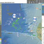
Gorda plate earthquake animations

I have put together a couple animations of the earthquake epicenters preceding, during, and following the recent earthquake swarm in the Gorda plate. Here is the first page I put together for this M 6.8 earthquake. Here are some maps I put together to explain the epicenter pattern and how it might relate to faults in the Gorda plate.
There was also a M 5.2 extensional earthquake in the Gorda rise (where the Gorda plate is created, it is like the Mid-Atlantic Ridge). Looking at the animations below, one may notice that there were a couple earthquakes in the region of this M 5.2 prior to the 2014 March Gorda Earthquake Swarm. While it may be considered that the Gorda earthquakes triggered the M 5.2, it is evident that the fault that slipped during the M 5.2 was probably getting ready to rupture. This is true for most triggered earthquakes. The change in stress on faults due to loading from other earthquakes is very very small compared to the amount of stress necessarily applied to a fault to cause rupture. In other words, a fault needs to be close to earthquake failure in order to be triggered by another earthquake. Also, that these triggered earthquakes are limited in time because the change in fault stress is short lived. The 2010 Rollins and Stein paper (downloadable here) discusses some coulomb stress modeling they did following the 2010 M 6.5 earthquake in the Gorda plate. Here is a paper that discusses how a Cascadia subduction zone earthquake could trigger an earthquake on the San Andreas fault.
I used the USGS website to download the epicenters in this region. One of the options is to export the epicenters as a google kml file. These files display in google earth.

Click on the maps to open/download the video in a new window.
Here is an animation of the region offshore northern California for the time range 2014/1/16 through 2014/3/23. (~23 MB avi)


Here is an animation zoomed into offshore of Humboldt County. The USGS fault and fold database show the faults. There are also plate boundary faults plotted (they are less certain and less precise). (~28 MB avi)


Here is an animation of the earthquake swarm itself. Note that there are some epicenters that strike at the same instance as the mainshock. These are probably all ruptures on the same fault. There are many other aftershocks that are not on the same fault, but synthetic (trend in a parallel or subparallel direction as the main fault) or antithetic faults (trend in a conjugate direction). In some cases there are also aftershocks that occur at the same instance and apparently align along another fault (they line up). For faults close to the mainshock fault, these aftershocks may actually be on the mainshock fault but are plotted incorrectly due to the assumptions made in the location inversions (i.e. velocity models). People like Mark Williams or Anne Trehu (among others) may want to do some double differencing to these data to get better locations for these earthquake hypocenters.


Here I have slowed down the animation to better visualize the temporal relations between bursts in seismic energy.


Finally, here is an animation of the western USA that reveals something about the random nature of background seismicity. There are a few locations that show patterns that suggest faults ruptured. The recent Gorda plate earthquake swarm is one example. There were also a series of epicenters that plot in a northeast strike/trend just west of the mouth of the Mattole River. There also appears to be a swarm of earthquakes in the Yellowstone region, the Geysers (CA), and Salinas, CA.

M 6.4 in the south Sandwich Islands (mmmm sandwich) 2014/3/11

While we were all excited about the local Gorda earthquake, there was an another interesting M 6.4 strike slip earthquake in the region of a recent series of earthquakes in the Scotia Sea. Sometimes earthquakes change the local stress field in the region of the earthquake and this may increase or decrease the stress of nearby faults. This “stress triggering” is short lived as the effects get spread out over time. The November 2013 earthquakes are recent enough that they may be blamed for triggering this M 6.4 earthquake, but that is pure speculation on my part. These fault systems are connected, but I have not done any modeling to determine if this is likely or not. One of the largest unknowns if he pre-earthquake stress on the fault that ruptured during this M 6.4 earthquake.
Please check out the pages I put together for the Scotia Sea earthquakes for more material on the regional tectonics here… There are some ascinating figures showing how this region was formed over the past few millions of years. The M 6.8 and M 7.8 earthquakes occurred along a strike slip fault system that links directly to the fault this M 6.4 earthquake may be located on. The M 7.0 earthquake occurred north of the M 6.8 and M 7.8, on another strike slip plate boundary fault. mmmm Sandwiches.

Here is a regional map showing the epicenter (in red and orange) with the plate boundary faults mapped in different colors.


Here is the Mww moment tensor for this earthquake. This shows the earthquake may be an east-west striking strike-slip earthquake, or a north-south striking strike slip earthquake.

Here is a local map showing the epicenter and the regional plate boundary faults. The largest orange dot is the epicenter for this M6.4 earthquake. There is an east-west green line that is a transform fault (strike-slip) nearest the epicenter. There are some north-south oriented faults (some magenta and some green). These are spreading ridges (extensional). Based on the tectonics here, I would interpret the moment tensor plotted above as a left-lateral strike slip earthquake.


Here is a regional map showing the modeled shaking intensity for this earthquake.


Here is the local map version of the shaking intensity map.


Here is a regional map showing the epicenter, along with a series of historic earthquake epicenters plotted as grey circles.


Here is the local map version of the epicentral map that includes the historic earthquakes.